modeling and simulations of railway vehicle systemthe railway vehicle running along a track is one...

55

Int. J. Mech. Eng. & Rob. Res. 2014 Rakesh Chandmal Sharma, 2014

MODELING AND SIMULATIONSOF RAILWAY VEHICLE SYSTEM

Rakesh Chandmal Sharma1*

This paper presents a 37-degree of freedom coupled vertical-lateral model of Indian Railwayvehicle formulated using Largrangian dynamics for the purpose of examining its dynamic behavior.The rail-vehicle for the present study is modeled as nine mass systems consisting of a carbody,two bolsters, two bogie frames and four wheel axle sets. The 37 coupled vertical-lateral motionequations are further utilized to investigate the ride behavior of Indian Railway General Sleeperand Rajdhani coach

Keywords: Lagrangian Dynamics, Degree of freedom, Track Roughness, Frequency responsefunction

INTRODUCTIONThe railway vehicle running along a track is oneof the most complex dynamical systems inengineering. It has many degrees of freedomand the study of rail vehicle dynamics is adifficult task. The travel of a rail vehicle on trackis always a coupled motion. There exists acoupling between vertical and lateral motions.The vertical irregularities of the track causeboth vertical and lateral vibrations in the railvehicle. In addition, the different rigid bodies,i.e., car body, bolsters, bogie frames and wheelaxles set execute different angular motions,i.e., roll, pitch and yaw which influence thedynamic behavior of the rail vehicle systemsignificantly. In developing the mathematicalmodel to study vertical response, it would notbe adequate to include bounce, pitch and rolldegrees of freedom of the components. On

ISSN 2278 – 0149 www.ijmerr.comSpecial Issue, Vol. 1, No. 1, January 2014

National Conference on “Recent Advances in MechanicalEngineering” RAME – 2014

© 2014 IJMERR. All Rights Reserved

Int. J. Mech. Eng. & Rob. Res. 2014

1 M M University, Mullana, Ambala, Haryana, India.

the other hand, for the lateral response model,it would not be sufficient to use lateral, yaw and

roll degrees of freedom of the components.There has been extensive work done various

researchers on the lateral and vertical

dynamics of the rail vehicle in order to studythese motions separately. Coupled vertical-

lateral motion of the rail vehicle has also beenstudied in past by Zhai et al. (1984) Goel et al.

(2005) and Kalker (1979). The present

research work is another effort in the samedirection.

Coupled vertical-lateral dynamics of four

wheeled road vehicle has been studied by

Nathoo and Healey (1978) (Meachem andAhlbeck, 1969) and of three-wheeled road

vehicle has been studied by Ramji (2004)using Largrangian approach.

Research Paper

56


In the present work a 37 degrees offreedom coupled vertical-lateral mathematicalmodel of an Indian Railway vehicle isformulated using Largangian dynamics and itsmotion has been studied. Both vertical andlateral irregularities of railway track areincorporated in the analysis and areconsidered as random function of time. Thesimulated results are compared with thevertical and lateral acceleration data obtainedthrough actual rail vehicle testing and the ridecomfort is evaluated using ISO 2631-1standards (1997).

MATHEMATICAL MODELINGVEHICLE MODELThe railway vehicle as shown in Figure 1comprises of a carbody supported by twobogies one at each end. Bolsters are theintermediate member between the carbodyand each bogie frame and is connected tocarbody through side bearings. The bogieframe supports the weight of the carbodythrough a secondary suspension locatedbetween the carbody and the bogie frame. Inpassenger vehicles, each bogie usuallyconsists of two wheel axle sets that areconnected through the primary suspension tothe bogie frame. In addition, the wheels areusually tapered or profiled to provide a selfcentering action as the axle traverses the track.The degrees of freedom assigned to thedifferent rigid bodies of a railway vehicle arementioned in Table 1. The inertial axes systemis fixed with the track while the origins of thebody fixed axes system are located at thecentre of mass of different rigid bodies e.g.car body, bolster, wheel axle etc. Themathematical model is formulated withfollowing assumptions.

Figure 1: Rail Vehicle Model

Table 1: Rigid Bodies and Their Degreesof Freedom

Components Motion

(Rigid Bodies) Lateral Vertical Roll Pitch Yaw

Carbody y1

z1

1

1

1

Front Bolster y2

z2

2

Rear Bolster y3

z3

3

Front Bogie y4

z4

4

4

4

Frame

Rear Bogie y5

z5

5

5

5

Frame

Front Bogie y6

z6

6

6

Front Wheel-Axle Set

Front Bogie y7

z7

7

7

Real Wheel-Axle Set

Rear Bogie y8

z8

8

8

Front Wheel-Axle Set

Rear Bogie y9

z9

9

9

Rear Wheel-Axle Set

57


• The rail vehicle possess longitudinal plane

of symmetry (i.e., center of gravity of all

masses lie in central plane).

• The vehicle is assumed to be traveling at

constant speed therefore degree of

freedom in longitudinal direction are not

assigned to the rigid bodies.

• All springs and dampers are assumed to

be linear

• Creep forces are assumed as linear

function of creepages (linear Kalkar’s theory

(Kalker, 1979) is utilized to calculate the

creep forces).

• Track is considered to be flexible.

• Car body is assumed to be rigid.

• Wheel and rail do not loose contact

The equations of motion describing coupled

vertical-lateral dynamics of the rail-vehicle are

obtained using the Lagrange’s equations,

which in general can be written as:

. .P D

ii i

i i

d L L E EQ

dt q qq q

... (1)

Largrangian L is defined as (T - Vg) where

T is the kinetic energy and Vgis the potential

energy due to gravity effect of the vehiclesystem, E

Pis the energy stored in the system

due to springs, EDis the Rayliegh’s dissipation

function of the system and Qi are the

generalized forces corresponding to iy thegeneralized coordinates.

The final equations of motion of rail vehicleare obtained in the following form

.. .

[ ]{ } [ ]{ } [ ]{ } [ ( )]i ri iM y C y K y F ...(2)

[M], [K] and [C] are the 37×37 mass,stiffness and damping matrices respectivelyfor rail vehicle. )]([ rF is a 37×1 force matrixfor displacement excitations at the eight wheelcontact points.

i.e., r = 1, 2….8, due to vertical and lateral trackirregularities.

TRACK MODELThe track may be divided into a super structureand a sub structure. The super structure includesrails, rail fastenings, pads, sleepers and ballast(i.e. soil). The sub grade or subsoil is the substructure of a track. The track in the presentanalysis is assumed to be flexible in bothvertical and lateral directions. Its flexibility isaccounted by considering wheel to be in serieswith sleeper, soil and subsoil (Figure 2) i.e.

1 1 1 1 1z z z z zR W SL S SSk k k k k ...(3)

and

1 1 1 1 1z z z z zR W SL S SSc c c c c ...(4)

similarly for lateral direction it can beassumed that

1 1 1 1 1y y y y yR W SL S SSk k k k k ...(5)

and

1 1 1 1 1y y y y yR W SL S SSc c c c c ...(6)

FREQUENCY RESPONSEFUNCTIONIn this analysis spectral densities of the output

variables are calculated directly from frequency

response functions and rail roughness spectral

58


densities. For computation of complexfrequency response function, harmonic inputis given at one wheel at a time while the inputsat the remaining wheels are kept zero. TheEquation (2) may also be written as

2([ ] ( ) [ ]( ) [ ])

[ ( )]

i ti

i tr r

M C i K y e

F q e

...(7)

The above equations may further be writtenas

1[ ] ( ) ( )r rD H F ...(8)

where [D1] is the dynamic stiffness matrix, and

Hr() = (y

i /q

r) is the complex frequency

response function for rth input. As the railwaytrack possesses both vertical and lateralirregularities, therefore in the present analysisboth vertical and lateral inputs are consideredand it is considered that the final response ofthe system is a combined effect due to verticaland lateral inputs from the track. Using theprinciple of superposition, the resultantcomplex frequency response is obtained bycombining the response matrices due to theeight inputs at the rail-wheel contact points.

REPRESENTATION OFTRACK ROUGHNESSThe irregularities in the railway track surface

are random and represented by power spectraldensity functions. In the present analysis autoand cross-power spectral density functions ofvertical and lateral irregularity for a straighttrack reported by Goel et al (2005) are used.Vertical and lateral irregularities, are of the typeS() = C

sp -N.C

sp is an empirical constant and

N characterizes the rate at which amplitudedecreases with frequency.

SYSTEM RESPONSE TOTRACK EXCITATIONThe vehicle response to random excitations

at the eight rail-wheel contact points has been

obtained using statistical approach. For a

multi-degree-of freedom lumped mass system,

using the concept of random vibrations, the

power spectral density for the response is

related to the excitation through the complex

frequency response function. Thus for a linear

system subjected to random inputs, using

input–output relationships for spectral

densities, the auto and cross-spectral density

matrix of the response may be written as

37 37 37 8 8 8 8 37[ ( )] [ ( )] [ ( )] [ ( )]Tyy r r rS H S H

...(9)

The complex frequency response functions[H

r()]

37×8 can also be defined as the ratio of

the response rate to unit harmonic input at agiven point. The superscript T denotestranspose of matrix.

It may be noted here that above equation isused independently for vertical and lateralirregularities of the track.

In the evaluation of vehicle ride quality, thePower Spectral Density (PSD) for theacceleration of the carbody mass center as a

Figure 2: Track Model

59


function of frequency is of prime interest. Themean square acceleration response (MSAR)expressed as (m/s2)2/Hz, which is nothing butPSD of acceleration may be written as

437 8 8 8 8 37(2 ) [ ( )] [ ( )] [ ( )]T

r r rMSAR f H S H

...(10)

The spectral density of output (or response)corresponding to each degree of freedom ofcarbody can be plotted against frequency withthe help of the above equation. To determineroot mean square acceleration response(RMSAR) at a center frequency f

c, power

spectral density function is integrated over aone third octave band i.e.

1.124 4

0.89

[(2 ) [ ( )]( ) ]fc

YY

fc

RMSAR sqrt S f f df

...(11)

The root mean square acceleration values

of acceleration both in vertical and lateraldirections of carbody mass center at a seriesof center frequencies within the range ofinterest is obtained and ride comfort isevaluated and compared with the specifiedISO 2631-1 standards (1997). In the presentanalysis principal frequency weightings withmultiplication factors specified in ISO 2631-1standards (1997) are applied to RMSacceleration values to obtain frequency-weighted acceleration for the evaluation ofpassenger comfort in sitting position.

The values of the parameters of a loadedGeneral Sleeper and Rajdhani coach of IndianRailways and of Indian railway track for presentanalysis are obtained from Research Designsand Standards Organisation, Lucknow (India).The values of creep coefficients for the wheel-track interaction have been obtained fromYuping and McPhee (2005). These values arementioned in Tables 2, 3 and 4.

Table 2: Values of Track Parameters and Creep Coefficients

Parameter Parameter Value Parameter Parameter Value

zSLk 65 MN/m y

SSk 50 MN/m

zSk 20 MN/m y

SLc 10 kN-sec/m

zSSk 35 MN/m y

Sc 50 kN-sec/m

zSLc 30 kN-sec/m y

SSc 70 kN-sec/m

zSc 40 kN-sec/m 11f 7.5848 x 106 N

zSSc 50 kN-sec/m 12f 1.5334 x 104 N

ySLk 50 MN/m 23f 61.56 N.m2

ySk 30 MN/m 33f 8.6605 x 106 N

60


RIDE BEHAVIOR FROMACTUAL TESTINGThe results from actual testings are obtainedfrom Research Designs Standards Organisation,

Table 3: Values of Rail Vehicle Parameters of Indian Railway General Sleeper ICF Coach

Parameter Parameter Parameter Parameter Parameter Parameter Parameter Parameter

Value Value Value Value

mc

37960 kg IBF

X 1546 kg m2 kBBF

z 0.42375 MN/m kW

y 250 MN/m

mB

400 kg IBF

Y 2893 kg m2 kBBf

y 0.2324 MN/m cW

y 4 MN-sec/m

mBF

2346 kg IBF

Z 4298 kg m2 cBBF

z 0.0589 MN-sec/m tC

0.8 m

mw

1487 kg IW

X 1181 kg m2 cBBF

y 1 MN-sec/m tB

1.127 m

IC

X 63950 kg m2 IW

Y 108.5 kg m2 kBFWA

z 0.26935 MN/m tW

1.079 m

IC

Y 1470750 kg m2 IW

Z 1181 kg m2 kBFWA

y 11.5 MN/m z12

1.3275 m

IC

Z 1473430 kg m2 kCB

z 35 MN/m cBFWA

z 0.0206 MN-sec/m z24

0.1435 m

IB

X 307 kg m2 kCB

y 17.5 MN/m cBFWA

y 0.5 MN-sec/m z46

0.194 m

IB

Y 00 cCB

z 0.035 MN-sec/m kW

z 1000 MN/m a 0.871 m

IB

Z 336.5 kg m2 cCB

y 0.0175 MN-sec/m cW

z 0.5 MN-sec/m 0.15 rad

Table 4: Values of Rail Vehicle Parameters of Indian Railway Rajdhani Coach

Parameter Parameter Parameter Parameter Parameter Parameter Parameter Parameter

Value Value Value Value

mc

33740 kg IBF

X 1713 kg m2 kBBF

z 0.42375 MN/m kW

y 250 MN/m

mB

400 kg IBF

Y 3206 kg m2 kBBf

y 0.2324 MN/m cW

y 4 MN-sec/m

mBF

2600 kg IBF

Z 4763 kg m2 cBBF

z 0.0589 MN-sec/m tC

0.8 m

mw

1600 kg IW

X 1271 kg m2 cBBF

y 1 MN-sec/m tB

1.127 m

IC

X 56932 kg m2 IW

Y 117 kg m2 kBFWA

z 0.26935 MN/m tW

1.079 m

IC

Y 1307220 kg m2 IW

Z 1271 kg m2 kBFWA

y 11.5 MN/m z12

1.3275 m

IC

Z 1309744 kg m2 kCB

z 35 MN/m cBFWA

z 0.0206 MN-sec/m z24

0.1435 m

IB

X 307 kg m2 kCB

y 17.5 MN/m cBFWA

y 0.5 MN-sec/m z46

0.194 m

IB

Y 00 cCB

z 0.0311 MN-sec/m kW

z 1000 MN/m a 0.871 m

IB

Z 336.4 kg m2 cCB

y 0.0175 MN-sec/m cW

z 0.5 MN-sec/m 0.15 rad

Lucknow. The rail vehicle is moved at aconstant speed of 80 km/h (General Sleeper)and 130 km/h (Rajdhani) over straight track.The data acquisition is completed in two

61


Figure 3: PSD of Vertical Accelerationof Loaded GS Coach (Actual Testing)

Figure 4: PSD of Lateral Accelerationof Loaded GS Coach (Actual Testing)

Figure 5: PSD of Vertical Accelerationof Loaded Rajdhani Coach

(Actual Testing)

Figure 6: PSD of Lateral Accelerationof Loaded Rajdhani Coach

(Actual Testing)

stages. In the first stage the record is obtainedfor 2 Km straight specimen run- down trackand this record is verified covering a long runof about 25 Km in the second stage. A straingauge accelerometer (Range: +1 g & +2 g;Frequency response: 25 Hz; Excitation: 5 VAC/DC; Sensitivity: 360 mV/V/g; Damping:silicon fluid) is placed at floor level near bogiepivot of the rail vehicle. The acceleration datais recorded in time domain with NationalInstruments cards (Sampling rate: 100Samples/s, Resolution: 12 Bit) using Lab Viewsoftware program and this record is convertedin frequency domain using Fast FourierTransformations (FFT).

Power spectral densities of accelerationsof loaded General Sleeper coach obtainedthrough actual testing in vertical and lateraldirections are shown in Figures 3 and 4

respectively and of loaded Rajdhani coach isshown in Figures 5 and 6 respectively.

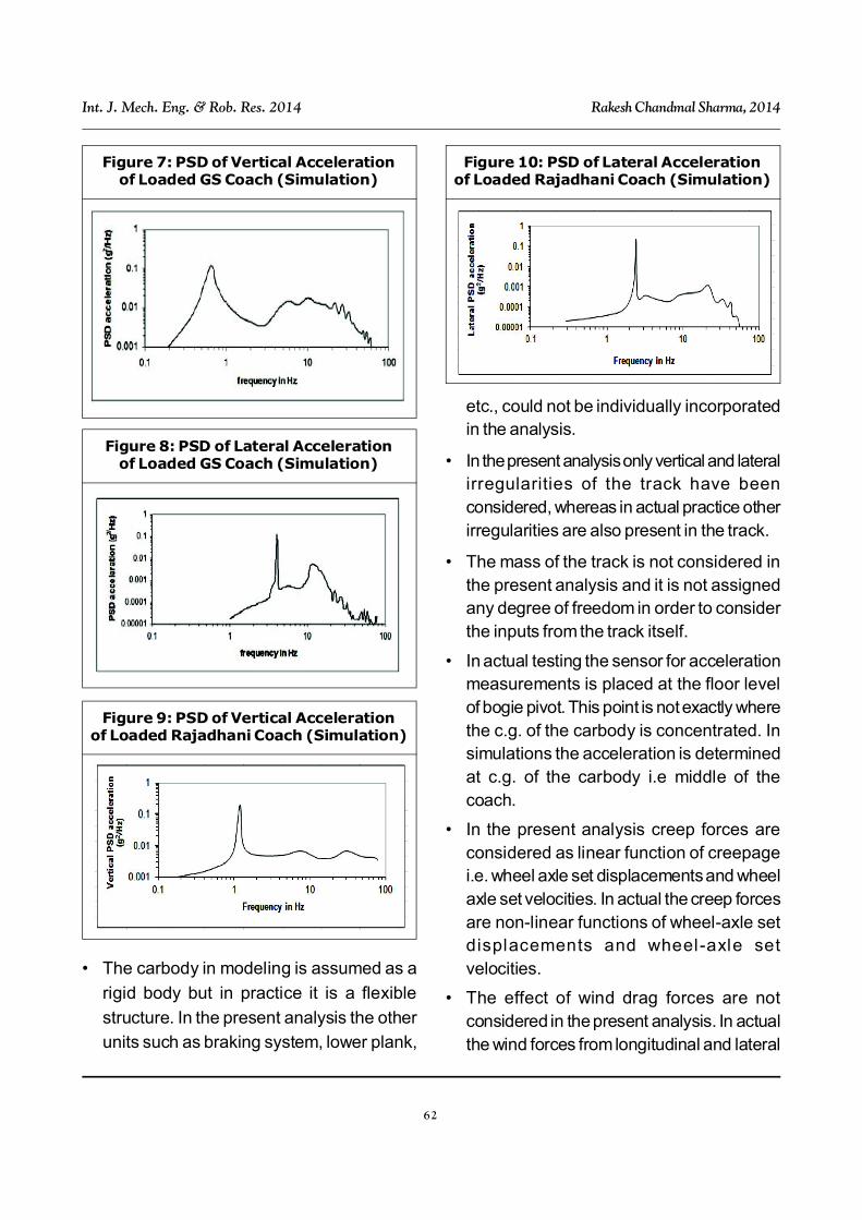
RIDE BEHAVIOR FROMSIMULATIONPower spectral densities of accelerations ofloaded carbody obtained through simulationin vertical and lateral directions are shown inFigures 7 and 8 (GS Coach) and Figures 9and 10 (Rajdhani coach). The theoretical andactual results compare reasonably well exceptthat the peak values are obtained at slightdifferent frequencies The actual and simulatedresults not being exactly similar is due to thefollowing facts:

62


etc., could not be individually incorporatedin the analysis.

• In the present analysis only vertical and lateralirregularities of the track have beenconsidered, whereas in actual practice otherirregularities are also present in the track.

• The mass of the track is not considered inthe present analysis and it is not assignedany degree of freedom in order to considerthe inputs from the track itself.

• In actual testing the sensor for accelerationmeasurements is placed at the floor levelof bogie pivot. This point is not exactly wherethe c.g. of the carbody is concentrated. Insimulations the acceleration is determinedat c.g. of the carbody i.e middle of thecoach.

• In the present analysis creep forces areconsidered as linear function of creepagei.e. wheel axle set displacements and wheelaxle set velocities. In actual the creep forcesare non-linear functions of wheel-axle setdisplacements and wheel-axle setvelocities.

• The effect of wind drag forces are notconsidered in the present analysis. In actualthe wind forces from longitudinal and lateral

Figure 8: PSD of Lateral Accelerationof Loaded GS Coach (Simulation)

Figure 9: PSD of Vertical Accelerationof Loaded Rajadhani Coach (Simulation)

Figure 10: PSD of Lateral Accelerationof Loaded Rajadhani Coach (Simulation)

Figure 7: PSD of Vertical Accelerationof Loaded GS Coach (Simulation)

• The carbody in modeling is assumed as a

rigid body but in practice it is a flexible

structure. In the present analysis the other

units such as braking system, lower plank,

63


CONCLUSIONThe result of vertical root mean square (RMS)acceleration response (Figure 11) indicatesthat the response of loaded GS coach lies wellwithin the ISO specifications (4 h comfortcriteria) except for frequency range from 5 to10.5 Hz. The result of lateral root mean square(RMS) acceleration response (Figure 12)indicates that the response of loaded GScoach lies well within the ISO specifications(4 h comfort criteria) except for frequency atnearly 4 Hz, where the peak value is obtained.The analysis indicates that discomfortfrequency range belongs from 4 to 10.5 Hz andimprovements in the rail vehicle design arerequired.

The result of vertical root mean square(RMS) acceleration response (Figure 13)indicates that the response of loaded Rajdhanicoach lies well within the ISO specifications(8 Hrs comfort criteria) except for frequency1.1 Hz and from frequency range from 5 to 10Hz. The result of lateral root mean square(RMS) acceleration response (Figure 14)indicates that the response of loaded Rajdhanicoach lies well within the ISO specifications(8 Hrs comfort criteria) except for frequency atnearly 2.5 Hz, where the peak value is

Figure 12: Lateral RMS Accelerationof Loaded GS Coach (Simulation)

Figure 13: Vertical RMS Accelerationof Loaded Rajadhani Coach (Simulation)

Figure 14: Lateral RMS Accelerationof Loaded Rajadhani Coach (Simulation)

Figure 11: Vertical RMS Accelerationof Loaded GS Coach (Simulation)

directions significantly affect the dynamicsof rail vehicle system.

The vertical and lateral RMS accelerationvalues of loaded GS coach obtained throughsimulation are shown in Figures 11 and 12 andof Rajdhani coach are shown in Figures 13and 14.

64


obtained. The analysis indicates thatdiscomfort frequency range belongs from 1 to10 Hz and improvements in the rail vehicledesign are required.

REFERENCES1. Garg V K and Dukkipatti V (1984),

Dynamics of Railway Vehicle Systems,Academic Press, New York.

2. Goel V K, Manoj Thakur, Kusum Deepand Awasthi B P (2005), “MathematicalModel to Represent the Track GeometryVariation using PSD”, Indian RailwayTechnical Bulletin, Vol. LXI, No. 312 –313, pp. 1-10.

3. ISO 2631: 1997, Mechanical Vibrationand Shock Evaluation of HumanExposure to Whole Body Vibrations-Part 1: General Requirements.

4. Kalker J (1979), “Survey of Wheel-RailContact Theory”, Vehicle SystemDynamics, No. 8, pp. 317-358.

5. Meachem H C and Ahlbeck D R (1969),“A Computer Study of Dynamic Loadscaused by Vehicle Track Interaction”, J.of Engg. for Industry. Trans. of theASME, Ser. B, Vol. 91, No. 3, pp. 808-816.

6. Nathoo N S and Healey A J (1978),

“Coupled Vertical-Lateral Dynamics of aPneumati c Ti red Vehi cl e: part 1- AMathematical Model”, Journal of Dynamic Syst em Measu rement andControl, Vol. 100, pp. 311-318.

7. Nathoo N S and Healey A J (1978),“Coupled Vertical-Lateral Dynamics of aPneumatic Tired Vehicle: part 2-Simulated verses Experimental Data”,Journal of Dynamic System Measurementand Control, Vol. 100, pp. 319-325.

8. Ramji K (2004), Coupled Vertical-Lateral Dynamics of Three-WheeledMotor Vehicles, Ph.D. Dissertation,Deptt of Mechanical and Industrial Engg.,I I T Roorkee.

9. Yuping H and McPhee J (2005),“Optimization of Curving Performance ofRail Vehicles”, Vehicle SystemDynamics, Vol. 43 No. 12, pp. 895-923.

10. Zhai W M, Cai C B and Guo S Z (1996),“Coupling Model of vertical and lateralvehicle/track interactions”, VehicleSystem Dynamics, Vol. 26, No.1, pp. 61-79.

11. Zhai W M, Wang K and Cai C (2009),“Fundamentals of vehicle-track coupleddynamics”, Vehicle System Dynamics,Vol. 47, No. 11, pp. 1349-1376.

65


APPENDIX

NOMENCLATURE

,C Bm Mass of carbody and bolster respectively

,BF Wm Mass of bogie frame and wheel axle respectively

, ,x y zCI Roll, pitch and yaw mass moment of inertia of carbody respectively

, ,x y zBI Roll, pitch and yaw mass moment of inertia of bolster respectively

, ,x y zBFI Roll, pitch and yaw mass moment of inertia of bogie frame respectively

, ,x y zWI Roll, pitch and yaw mass moment of inertia of wheel axle respectively

,z yCBk Vertical (½ part) and lateral (½ part) stiffness between carbody and bolster

respectively

,z yCBc Vertical (½ part) and lateral (½ part) damping coefficient between carbody and

bolster respectively

,z yBBFk Vertical (¼ part) and lateral (½ part) stiffness between bolster and bogie frame

respectively

,z yBBFc Vertical and lateral damping coefficient between bolster and bogie frame

respectively (½ part)

,z yBFWAk Vertical (¼ part) and lateral (½ part) stiffness between bogie frame and

corresponding wheel axle

,z yBFWAc Vertical (¼ part) and Lateral (½ part) damping coefficient between bogie frame

and corresponding wheel axle

,z yRk Vertical and lateral stiffness of rail respectively

,z yRc Vertical & lateral damping coefficient of rail respectively

Wt Lateral distance from bogie frame c.g. to corresponding vertical suspension

between bogie frame and wheel axle

66


Ct Lateral distance from carbody c.g. to side bearings

Bt Lateral distance from bolster c.g. to vertical suspension between bolster and

bogie frame

12z Vertical distance between carbody c.g. and bolster c.g.

24z Vertical distance between bolster c.g. and bogie frame c.g

46z Vertical distance between bogie frame c.g. and corresponding wheel axle c.g.

a Half of wheel gauge

APPENDIX (CONT.)

modeling and simulations of railway vehicle systemthe railway vehicle running along a track is one...

Documents