modeling bivariate lorenz curves with applications to ... extension of the univariate lorenz curve...
TRANSCRIPT

Fifth meeting of the Society for the Study of Economic Inequality ECINEQBari, Italy, July 22-24, 2013
Modeling Bivariate Lorenz Curves with
Applications to Multidimensional Inequality
in Well-Being
Jose Marıa Sarabia1, Vanesa Jorda
Department of Economics, University of Cantabria, 39005-Santander, Spain
Updated version 10th June 2013
Abstract
The extension of the univariate Lorenz curve to higher dimensions isnot an obvious task. The three existing definitions were proposed byTaguchi (1972a,b), Arnold (1983) and Koshevoy and Mosler (1996),who introduced the concepts of Lorenz zonoid and Gini zonoid index.In this paper, using the definition proposed by Arnold (1983), closedexpressions for the bivariate Lorenz curve are given, assuming differ-ent formulations of the underlying bivariate income distribution. Westudy a relevant type of models based on the class of bivariate distri-butions with given marginals described by Sarmanov and Lee (Lee,1996; Sarmanov, 1966). This model presents several advantages, inparticular the expression of the bivariate Lorenz curve can be easilyinterpreted as a convex linear combination of products of classical andconcentrated Lorenz curves. A closed expression for the bivariate Giniindex (Arnold, 1987) in terms of the classical and concentrated Giniindices of the marginal distributions is given. This index is speciallyuseful, and can be decomposed in two factors, corresponding to theequality within and between variables. Specific models with Beta,GB1, Pareto, Gamma and lognormal marginal distributions are stud-ied. Other alternative families of bivariate Lorenz curves are discussed.Some concepts of stochastic dominance are explored. Extensions tohigher dimensions are included. Finally, an application to measure-ment multidimensional inequality in well-being is given.
1Corresponding author. Tel.: +34-942-201635; Fax: +34-942-201603. E-mail address:[email protected] (J.M. Sarabia).
1

Key Words: bivariate Lorenz curve; Sarmanov-Lee distribution; bivariateGini index; Stochastic dominance; well-being
1 Introduction
The present economic research have stressed the importance of using morethan one attribute in the study of economic inequality. The different works byAtkinson (2003), Atkinson and Bourguignon (1982), Kolm (1977), Maasoumi(1986), Slottje (1987) and Tsui (1995, 1999) move in this direction.
In the last decades academics’ interest in assessing country levels of well-being has shifted from income alone to a more comprehensive conception ofsuch a process, which has an intrinsic multidimensional nature. In fact, thereis nearly consensus that income is not an adequate indicator of well-being(see e.g. Sen (1988, 1989, 1999)), thus other factors need to be taken intoaccount to evaluate this phenomenon effectively. Different approaches havebeen proposed in the literature to measure inequality in well-being, being themost satisfactory one the consideration multidimensional inequality measuressince this methodology takes into account inequality within each dimensionand the degree of association among them. However, as in the unidimensionalcase, these measures only offer overall conclusions about the evolution ofwell-being distribution, thus other statistical tools are needed to analyse theevolution of inequality in different parts of the distribution.
In this context, the extension of the univariate Lorenz curve to higherdimensions is not an obvious task. The three existing definitions were pro-posed by Taguchi (1972a,b), Arnold (1983) and Koshevoy and Mosler (1996),who introduced the concepts of Lorenz zonoid and Gini zonoid index.
In this paper, using the definition proposed by Arnold (1983), closedexpressions for the bivariate Lorenz curve are given, assuming different for-mulations of the underlying bivariate income distribution. We study a rele-vant type of models based on the class of bivariate distributions with givenmarginals described by Sarmanov and Lee (Lee, 1996; Sarmanov, 1966). Thismodel presents several advantages, in particular the expression of the bivari-ate Lorenz curve can be easily interpreted as a convex linear combination ofproducts of classical and generalized Lorenz curves. A closed expression forthe bivariate Gini index (Arnold, 1987) in terms of the classical and general-ized Gini indices of the marginal distributions is given. This index is speciallyuseful, and can be decomposed in two factors, corresponding to the equal-
2

ity within and between variables. Specific models with Beta, GB1, Pareto,Gamma and lognormal marginal distributions are studied. Other alternativefamilies of bivariate Lorenz curves are discussed. Some concepts of stochas-tic dominance are explored. Extensions to higher dimensions are included.An application to measurement multidimensional inequality in well-being isgiven.
The contents of the paper are the following. In Section 2 we presentpreliminary results including the definition of univariate Lorenz and con-centration curves and a short review about the three different definitions ofbivariate Lorenz curves proposed in the literature. In Section 3 we introducethe bivariate Sarmanov-Lee Lorez curve, where we obtain a nice closed ex-pression, as well as a closed expression for the corresponding bivariate Giniindex, according to the Arnold’s (1987) definition. A decomposition of thisindex in two factors is given, which correspond to the equality within andbetween variables. Different models of bivariate Lorenz curves are presentedin Section 4. Stochastic ordering are discussed in Section 5. Extension tohigher dimensions are discussed in Section 6. An application to measurementmultidimensional inequality in well-being is given in Section 7. Finally, someconclusions are given in Section 8.
2 Preliminary Results
2.1 Univariate Lorenz and Concentration Curves
We denote the class of univariate distributions functions with positive fi-nite expectations by L and denote by L+ the class of all distributions in Lwith F (0) = 0 corresponding to non-negative random variables. We use thefollowing definition by Gastwirth (1971).
Definition 1 The Lorenz curve L of a random variable X with cumulativedistribution function F ∈ L is,
L(u;F ) =
u∫0
F−1(y)dy
1∫0
F−1(y)dy
=
u∫0
F−1(y)dy
E[X], 0 ≤ u ≤ 1, (1)
3

where
F−1(y) = supx : F (x) ≤ y, 0 ≤ y < 1,
= supx : F (x) < 1, y = 1,
is the right continuous inverse distribution function or quantile function cor-responding to F .
Now, we present the concept of concentration curve introduced by Kak-wani (1977). Let g(x) be a continuous function of x such that its first deriva-tive exists and g(x) ≥ 0. If the mean EF [g(X)] exits, then one can define
Lg(y;F ) =
∫ x0g(x)dF (x)
EF [g(X)]
where y = g(x) and f(x) and F (x) are respectively the probability densityfunction (PDF) and the cumulative distribution function (CDF) of the ran-dom variable X. The implicit relation between Lg(g(x);F ) and F (x) willbe called the concentration curve of the function g(X). If ηg(x) and ηg∗(x)denote the elasticities of g(x) and g∗(x), the concentration curve for the func-tion g(x) will lie above (below) the concentration curve for the function g∗(x)if ηg(x) is less (greater) than ηg∗(x) for all x ≥ 0. The concentration curveadmits the simple explicit representation,
Lg(u;F ) =1
EF [g(X)]
u∫0
g[F−1(t)]dt,
which will be used in the next Sections.
2.2 The three different definitions of Bivariate Lorenzcurve
In this section we discuss briefly the three definitions proposed in the liter-ature for constructing a bivariate Lorenz curve. These definitions were sug-gested by Taguchi (1972a,b), Arnold (1983, 1987) and Koshevoy and Mosler(1996). We consider the bivariate definition, which can be extend to higherdimensions.
4

2.2.1 The Taguchi’s (1972) definition of bivariate Lorenz curve
This definition was the first proposal in the literature of bivariate Lorenzcurve.
Definition 2 The Lorenz surface of F12 is the set of points (s, t, L(s, t)) inR3
+ defined by,
s =
u∫0
v∫0
f12(x1, x2)dx1dx2, t =
u∫0
v∫0
x1f12(x1, x2)dx1dx2
E[X1],
L(s, t;F12) =
u∫0
v∫0
x2f12(x1, x2)dx1dx2
E[X2].
This definition was investigated by Taguchi (1972a,b, 1988). The defini-tion is not symmetric in (s, t), and its extension to higher dimensions doesnot look simple.
2.2.2 Arnold’s (1983, 1987) definition of bivariate Lorenz curve
The following definition was proposed by Arnold (1983, 1987) and it is anextension of (1) quite natural to higher dimensions. Let X = (X1, X2)> bea bivariate random variable with bivariate probability distribution functionF12 on R2
+ having finite second and positive first moments. We denote by Fi,i = 1, 2 the marginal CDF corresponding to Xi, i = 1, 2 respectively.
Definition 3 The Lorenz surface of F12 is the graph of the function,
L(u1, u2;F12) =
s1∫0
s2∫0
x1x2dF12(x1, x2)
∞∫0
∞∫0
x1x2dF12(x1, x2)
, (2)
where
u1 =
∫ s1
0
dF1(x1), u2 =
∫ s2
0
dF2(x2), 0 ≤ u, v ≤ 1.
5

The two-attribute Gini-Arnold index GA(F12) is defined as,
GA(F12) = 4
1∫0
1∫0
[u1u2 − L(u1, u2;F12)]du1du2, (3)
where the egalitarian surface is given by L0(u1, u2;F0) = u1u2. Previousdefinition has not been explored in detail in the literature. We highlightsome of its properties:
1. The marginal Lorenz curves can be obtained as L(u1;F1) = L(u1,∞;F12)and L(u2;F2) = L(∞, u2;F12).
2. The bivariate Lorenz curve does not depend on changes of scale in themarginals.
3. If F12 is a product distribution function, then
L(u1, u2;F12) = L(u1;F1)L(u2;F2),
which is just the product of the marginal Lorenz curves.
4. We denote by Fa the one-point distribution at a ∈ R2+, that is, the
egalitarian distribution at a. Then, the egalitarian distribution hasbivariate Lorenz curve L(u1, u2;Fa) = u1u2.
5. In the case of a product distribution, the two-attribute Gini-Arnolddefined in (3) can be written as,
1−GA(F12) = [1−G(F1)][1−G(F2)].
The Arnold’s Lorenz curve can be evaluated implicitly in some relevantbivariate families of income distributions. We consider the following model.
Example 1 Let X = (X1, X2)> be a bivariate second kind beta distribution(or inverted beta distribution) with joint PDF,
f(x1, x2;α) = K(α1, α2, α3)xα1−1
1 xα2−12
(1 + x1 + x2)α1+α2+α3, x1, x2 ≥ 0, (4)
where K(α1, α2, α3) = Γ(α1+α2+α3)Γ(α1)Γ(α2)Γ(α3)
, αi > 0, i = 1, 2, 3. The marginals are
second kind beta distributions: X1 ∼ B2(α1, α3) and X2 ∼ B2(α2, α3), with
6

PDF f(x; p, q) = 1B(p,q)
xp−1/(1 + x)p+q. The second kind beta distribution is
very common in inequality analysis (see Chotikapanich et al, 2007) and it isa subfamily of the GB2 distribution (McDonald, 1984). The joint CDFs of(4) is (see Balakrishnan and Lai, 2009),
F (x1, x2;α1, α2, α3) = K(α1, α2, α3)xα11 x
α22 H[x1, x2;α1, α2, α3], (5)
where K(α1, α2, α3) = K(α1,α2,α3)α1α2
and
H[x1, x2;α1, α2, α3] = F2[α1 + α2 + α2;α1, α2;α1 + 1, α2 + 1;−x1,−x2],
where F2 is the Appell’s hypergeometric function of two variables, defined as(Bailey, 1935)
Γ(β)Γ(β′)Γ(γ − β)Γ(γ′ − β′)Γ(γ)Γ(γ′)
F2[α;β, β′; γ, γ′;x, y]
=
∫ 1
0
∫ 1
0uβ−1vβ
′−1(1− u)γ−β−1(1− v)γ′−β−1(1− ux− vy)−αdudv.
The product moment of (4) is E[X1X2] = α1α2
(α3−1)(α3−2), which exists if α3 >
2. The bivariate Lorenz curve is defined implicitly by (u1, u2, L(u1, u2;F12))where,
L(u1, u2;F12) = F [s1, s2;α1 + 1, α2 + 1, α3 − 2],
where ui = Fi(si), i = 1, 2, α3 > 2 and F [., .; ., ., .] is defined in (5).
2.2.3 The Koshevoy and Mosler (1996) Lorenz Curve
The following definition of Lorenz curve was initially proposed by Koshevoy(1995), were this author identifies the suitable definition. Then, the restof results were obtained by Koshevoy and Mosler (1996, 1997) and Mosler(2002). Denote by L2
+ de set of all 2-dimensional non-negative random vec-tors X with finite positive marginal expectations. Let Ψ(2) denote the classof all measurable functions from R2
+ to [0, 1].
Definition 4 Let X ∈ L2+. The Lorenz zonoid L(X) of the random vector
X = (X1, X2)> with distribution F12 is defined as,
L(X) =
(∫ψ(x)dF12(x),
∫x1ψ(x)
E[X1]dF12(x),
∫x2ψ(x)
E[X2]dF12(x)
): ψ ∈ Ψ(2)
,
=
(E[ψ(X)],
E[X1ψ(X)]
E[X1],E[X2ψ(X)]
E[X2]
): ψ ∈ Ψ(2)
.
7

The Lorenz zonoid if a convex American football-shaped subset of the3-dimensional unit cube that includes the points (0, 0, 0) and (1, 1, 1). Ex-tension to higher dimensions is quite direct. However, the computation ofthese formulas in parametric income distributions is not easy.
3 The bivariate Sarmanov-Lee Lorenz Curve
In this section we introduce the so-called bivariate Sarmanov-Lee Lorenzcurve. As a previous step, we introduce an explicit expression for the Arnold’sbivariate LC an the bivariate Sarmanov-Lee distribution.
3.1 Explicit expression for the Arnold’s (1983) bivari-ate Lorenz curve
Many of our results are based on a explicit expression of the bivariate Lorenzcurve defined in (2). The bivariate Lorenz curve (2) admits the followingsimple explicit representation,
Lemma 1 The bivariate Lorenz curve can be written in the explicit form,
L(u1, u2;F12) =1
E[X1X2]
u1∫0
u2∫0
A(x1, x2)dx1dx2, 0 ≤ u1, u2 ≤ 1, (6)
where
A(x1, x2) =F−1
1 (x1)F−12 (x2)f12(F−1
1 (x1), F−12 (x2))
f1(F−11 (x1))f2(F−1
2 (x2)). (7)
Proof: The proof is direct making the change of variable (u1, u2) =(F1(x1), F2(x2)) in (2).
3.2 The bivariate Sarmanov-Lee Distribution
Let X = (X1, X2)> be a bivariate Sarmanov-Lee (SL) distribution with jointPDF,
f(x1, x2) = f1(x1)f2(x2) 1 + wφ1(x1)φ2(x2) , (8)
8

where f1(x) and f2(y) are the univariate PDF marginals, φi(t), i = 1, 2 arebounded nonconstant functions such that,
∞∫−∞
φi(t)fi(t)dt = 0, i = 1, 2,
and w is a real number which satisfies the condition 1+wφ1(x1)φ2(x2) ≥ 0 forall x1 and x2. We denote µi = E[Xi] =
∫∞−∞ tfi(t)dt, i = 1, 2, σ2
i = var[Xi] =∫∞−∞(t − µi)2fi(t)dt, i = 1, 2 and νi = E[Xiφi(Xi)] =
∫∞−∞ tφi(t)fi(t)dt, i =
1, 2. Properties of this family has been explored by Lee (1996). Momentsand regressions of this family can be easily obtained. The product momentis E[X1X2] = µ1µ2 + wν1ν2, and the regression of X2 on X1 is given by
E[X2|X1 = x1] = µ2 + wν2φ1(x1).
The copula associated to (8) is,
C(u1, u2;w, φ) = u1u2 +
u1∫0
u2∫0
φ1(s1)φ2(s2)ds1ds2,
where φi(si) = φi(F−1i (si), i = 1, 2, and Fi(xi) are the CDF of X. The PDF
of the copula associated to (8) is,
c(u1, u2;w, φ) =∂C(u1, u2;w, φ)
∂u1∂u2
= 1 + wφ1(F−11 (u1))φ2(F−1
2 (u2)).
Note that (8) and its associated copula has two components: a first compo-nent corresponding to the marginal distributions and the second componentwhich defines the structure of dependence, given by the parameter w andthe functions φi(u), i = 1, 2. These two components will be translated tothe structure of the associated bivariate Lorenz curve, and the correspondingbivariate Gini index.
In relation with other copulas, the Sarmanov-Lee copula has several ad-vantages: its joint PDF and CDF are quite simple; the covariance structure ingeneral is not limited and its different probabilistic features (moments, condi-tional distributions...) can be obtained in a explicit form. On the other hand,the SL distribution includes several relevant special cases including the clas-sical Farlie-Gumbel-Morgenstern distribution, and the variations proposedby Huang and Kotz (1999) and Bairamov and Kotz (2003).
9

3.3 The bivariate SL Lorenz Curve
The bivariate SL Lorenz curve is obtained using (8) in definition (2)
Theorem 1 Let X = (X1, X2)> a bivariate Sarmanov-Lee distribution withjoint PDF (8) with non-negative marginals satisfying E[X1] < ∞, E[X2] <∞ and E[X1X2] <∞. Then, the bivariate Lorenz curve is given by,
LSL(u1, u2;F12) = πL(u1;F1)L(u2;F2) + (1− π)Lg1(u1;F1)Lg2(u2;F2), (9)
whereπ =
µ1µ2
E[X1X2]=
µ1µ2
µ1µ2 + wν1ν2
,
and L(ui;Fi), i = 1, 2 are the Lorenz curves of the marginal distributionXi, i = 1, 2 respectively, and Lgi(ui;Fi), i = 1, 2 represent the concentrationcurves of the random variables gi(Xi) = Xiφi(Xi), i = 1, 2, respectively.
Proof: The function (7) for the Sarmanov-Lee distribution can be writtenof the form,
ASL(x1, x2) = F−11 (x1)F−1
2 (x2)
1 + wφ1(F−11 (x1))φ2(F−1
2 (x2)),
and integrating in the domain (0, u)× (0, v) we obtain,
µ1µ2L(u1;F1)L(u2;F2) + wEF1 [g1(X1)]EF2 [g2(X2)]Lg1(u1;F1)Lg2(u2;F2),
and after normalized we obtain (9).The interpretation of (9) is quite direct: the bivariate Lorenz curve can be
written as a convex linear combination of two components: (a) a first compo-nent corresponding to the product of the marginal Lorenz curves (marginalcomponent) and a second component corresponding to the product of theconcentration Lorenz curves (structure dependence component).
3.4 Bivariate Gini index
The following result provides a convenient write of the two-attribute bivariateGini defined in (3). This expression permits a simple decomposition of theequality in two factors: a first factor which represent the equality withinvariables and a second factor which represent the equality between variables.
10

Theorem 2 Let X = (X1, X2)> be a bivariate Sarmanov-Lee distributionwith bivariate Lorenz curve L(u, v;F12). The two-attribute bivariate Giniindex defined in (3) is given by,
1−G(F12) = π[1−G(F1)]·[1−G(F2)]+(1−π)[1−Gg1(F1)]·[1−Gg2(F2)], (10)
where G(Fi), i = 1, 2 are the Gini indices of the marginal Lorenz curves,and Ggi(Fi), i = 1, 2 represent the concentration indices of the concentrationLorenz curves Lgi(ui, Fi), i = 1, 2.
Proof: The proof is direct using expression (9) and taking into account
that G(F12) = 1− 4∫ 1
0
∫ 1
0L(u, v;F12)dudv.
Then the overall equality (OE) given by 1 − G(F12) can be decomposedin two factors,
OE = WE +BE, (11)
where
OE = 1−G(F12),
WE = π[1−G(F1)][1−G(F2)],
BE = (1− π)[1−Gg1(F1)][1−Gg2(F2)],
and WE represents the equality within variables and the second factor BErepresent the equality between variables. Note that the decomposition iswell defined (since 0 ≤ OE ≤ 1 and 0 ≤ WE ≤ 1 and in consequence0 ≤ BE ≤ 1) and BE includes the structure of dependence of the underlyingbivariate income distribution through the functions gi, i = 1, 2.
4 Bivariate Lorenz curve Models
In this section we consider several relevant models based on the previousmethodology.
4.1 Bivariate Pareto Lorenz curve based on the FGMfamily
Let X = (X1, X2)> be a bivariate FGM with classical Pareto marginals andjoint PDF,
f12(x1, x2;α, σ) = f1(x1)f2(x2)1 + w[1− 2F1(x1)][1− 2F2(x2)], (12)
11

where
Fi(xi) = 1−(x
σi
)−αi
, xi ≥ σi, i = 1, 2,
fi(xi) =αiσi
(x
σi
)−αi−1
, xi ≥ σi, i = 1, 2
are the CDF and the PDF respectively, of the classical Pareto distributions(Arnold, 1983), with αi > 1, σi > 0, i = 1, 2, −1 ≤ w ≤ 1 and φi(xi) =1− 2Fi(xi), i = 1, 2.
Using (9) with gi(xi) = xi[1− 2Fi(xi)], i = 1, 2 and after some computa-tions, the bivariate Lorenz curve associated to (12) is,
LFGM(u1, u2;F12) = πwL(u1;α1)L(u2;α2) + (1− πw)Lg1(u1;α1)Lg2(u2;α2),(13)
whereL(ui;αi) = 1− (1− ui)1−1/αi , 0 ≤ u ≤ 1, i = 1, 2,
and
Lgi(ui;αi) = 1− (1− ui)1−1/αi [1 + 2(αi − 1)ui], 0 ≤ u ≤ 1, i = 1, 2,
and,
πw =(2α1 − 1)(2α2 − 1)
(2α1 − 1)(2α2 − 1) + w.
The bivariate Gini index is given by,
G(α1, α2) =(3α1 − 1)(3α2 − 1)(2α1 + 2α2 − 3) + [h(α1, α2)]w
(3α1 − 1)(3α2 − 1)[(1− 2α1)(1− 2α2) + w],
where
h(α1, α2) = −3− 4α21(α2 − 1)2 + (5− 4α2)α2 + α1(5 + α2(8α2 − 7)).
The FGM bivariate distribution has a correlation structure limited, thatis |ρ(X1, X2)| ≤ 1
3, and in consequence, models (??) and (13) must be used
for income data configurations with moderate correlation.The following classes of models do not present this inconvenient.
12

4.2 Bivariate Sarmanov-Lee Lorenz curves with Betaand GB1 Marginals
Let Xi ∼ Be(ai, bi), i = 1, 2 be two classical beta distributions with PDF,
fi(xi; ai, bi) =xai−1i (1− xi)bi−1
B(ai, bi), 0 ≤ xi ≤ 1, i = 1, 2
where B(ai, bi) = Γ(ai)Γ(bi)/Γ(ai + bi), for i = 1, 2. This distribution hasbeen proposed as a model of income distribution by McDonald (1984) andmore authors. If we consider the mixing functions φi(xi) = xi − µi, whereµi = E[Xi] = ai/(ai + bi), i = 1, 2, the bivariate SL distribution is,
f12(x1, x2) = f1(x1; a1, b1)f2(x2; a2, b2)
1 + w
(x1 −
a1
a1 + b1
)(x2 −
a2
a2 + b2
),
(14)where w satisfies,
−(a1 + b1)(a2 + b2)
maxa1a2, b1b2≤ w ≤ (a1 + b1)(a2 + b2)
maxa1b2, a2b1.
A good property of this family is that it can be expressed as a linear combi-nation of products of univariate beta densities.
The univariate Lorenz curve of the univariate classical beta distributionif given by (Sarabia, 2008),
L(ui;Fi) = GBe(ai+1,bi)[G−1Be(ai,bi)(ui)], i = 1, 2, (15)
where GBe(a,b)(z) = (1/B(a, b))z∫0
ta−1(1 − t)b−1dt represents the CDF of a
classical Beta distribution. In consequence, the concentration curve can bewritten as,
Lgi(ui;Fi) =E[X2
i ]GBe(ai+2,bi)(G−1Be(ai,bi)(ui))− E[Xi]
2L(ui;Fi)
var[Xi], i = 1, 2.
(16)Note that νi = EFi
[Xiφi(Xi)] = var[Xi], i = 1, 2. Finally, combining (15)with (16) in (9), we obtain the bivariate beta Lorenz curve.
This model can be extended easily to the SL distribution with generalizedbeta of the first type (GB1) marginals, with PDF,
f(xi; ai, bi, pi) =pix
aipi−1i (1− xpii )bi−1
B(ai, bi), 0 ≤ xi ≤ 1, i = 1, 2,
13

and mixing function,
φi(xi) = xi − µi = xi −Γ(ai + 1/pi)Γ(ai + bi)
Γ(ai + bi + 1/pi)Γ(ai), i = 1, 2.
4.3 Bivariate SL Lorenz curves with Gamma Marginals
Let Xi ∼ G(αi, λi), i = 1, 2 be classical gamma distributions with PDFfi(xi) = λαi
i xαi−1i e−λixi/Γ(αi), where xi > 0 and αi, λi > 0, i = 1, 2. If we
consider the mixing function φi(xi) = e−xi − L(1;αi, λi), where L(s, α, λ) =(1 + s/λ)−α is the Laplace transform of a gamma distributions (Lee, 1996),we can construct the SL distribution with gamma marginals defined as,
f(x1, x2) = f1(x1)f2(x2)
1 + w(e−x1 − L(1;α1, λ1)
) (e−x2 − L(1;α2, λ2)
),
(17)with x1, x2 > 0. Note that (17) can be written as a linear combination ofproducts of univariate gamma distributions. Then, if we define,
gi(xi) = xie−xi − xiL(1;αi, λi), i = 1, 2,
the bivariate SL Lorenz curve with gamma marginals is,
LG(u1, u2;F12) = πL(u1;F1)L(u2;F2) + (1− π)Lg1(u1;F1)Lg2(u2;F2),
whereL(ui;Fi) = Hαi+1[H−1
αi(ui)], i = 1, 2,
and
Lgi(ui;Fi) =(1 + λi)
−1Hαi+1[(1 + 1λi
)H−1αi
(ui)]− λ−1i Hαi+1[H−1
αi(ui)]
(1 + λi)−1 − λ−1i
, i = 1, 2,
being Hα(x) =∫ x
0tα−1e−tdt/Γ(α) the CDF of a classical gamma distribution.
4.4 Distributions with lognormal marginals
The lognormal distribution plays an important role in the analysis of incomeand wealth data. There are several classes of bivariate distributions withlognormal distributions. Perhaps, the most natural definition of bivariatelognormal distribution is given in terms of a monotone marginal transforma-tion of the classical bivariate normal distribution. Other alternatives have
14

been described by Sarabia et al (2007). In these cases we can obtain a bi-variate Lorenz curve using the Arnold’s definition. If Xi ∼ LN (µXi
, σ2Xi
),i = 1, 2 denote a lognromal distribution, it is possible to consider a SL dis-tribution with lognormal marginals, where the mixing functions are definedby,
φi(xi) = fi(xi)−∞∫
0
f 2i (xi)dxi
= fi(xi)−1
2σXi
√π
exp
(−µXi
+σ2Xi
4
), i = 1, 2.
Now, if gi(xi) = xiφi(xi) = xifi(xi) − xi∫∞
0f 2i (xi)dxi, i = 1, 2 we can use
expression (9) for obtaining the corresponding bivariate Lorenz curve.
4.5 Other classes of bivariate Lorenz curves
Other alternative families of bivariate Lorenz curves can be construted, in-cluding models with marginals specified in terms of univariate Lorenz curves(see Sarabia et al., 1999) and models based on mixture of distributions (seeSarabia et al, 2005), which permits to incorporate heterogeneity factors inthe inequality analysis.
5 Stochastic Orderings
In this section we study some stochastic orderings related with the Lorenzcurves previously defined.
5.1 The univariate case
The usual Lorenz ordering is given in the following definition.
Definition 5 Let X, Y ∈ L with CDFs FX and FY and Lorenz curvesL(u;FX) and L(u;FY ), respectively. Then, X is less than Y en the Lorenzorder denoted by X L Y if L(u;FX) ≥ L(u;FY ), for all u ∈ [0, 1].
A similar definition for concentration curves can also be considered.
15

5.2 The general case
We denote by Lk+ the set of all k-dimensional nonnegative random vectorsX and Y with finite marginal expectations, that is E[Xi] ∈ R++. We definethe following orderings (Marshall, Olkin and Arnold, 2011)
Definition 6 Let X,Y ∈ Lk+, and we define the orders
(i) X L Y if L(u;FX) ≥ L(u;FY),
(ii) X L1 Y if E[g(
X1
E[X1], . . . , Xk
E[Xk]
)]≤ E
[g(
Y1E[Y1]
, . . . , YkE[Yk]
)], for ev-
ery continuous convex function g : Rk → R for which expectationsexists,
(iii) X L2 Y if∑k
i=1 aiXi L∑k
i=1 aiYi for every a ∈ Rk
(iv) X L3 Y if∑k
i=1 biXi L∑k
i=1 biYi for every b ∈ Rk+
(v) X L4 Y if Xi L Yi, i = 1, 2, . . . , k
It can be verified (Marshall, Olkin and Arnold, 2011) that L1⇒L2 andL2⇔L⇒L3⇒L4. We have the next theorem.
Theorem 3 Let X,Y ∈ L2+ with the same Sarmanov-Lee copula. Then, if
Xi L Yi, and Xi Lgi Yi i = 1, 2, then X L Y.
Proof: The proof is direct based on the expression of the bivariateSarmanov-Lee Lorenz curve defined in (9).
6 Extensions to higher dimensions
In this section we discuss briefly how to extend the results in previous sectionsto dimensions higher than two. First, we consider the general definition ofLorenz curve (2). Let X = (X1, . . . , Xm)> be a random vector in Lm+ withjoint CDF F12...m(x1, . . . , xm). The multivariate Arnold’s Lorenz curve canbe defined as,
L(u;F12...m) =
s1∫0
. . .sm∫0
m∏i=1
xidF12...m(x1, . . . , xm)
E
[m∏i=1
Xi
] ,
16

where ui =si∫0
dFi(xi), i = 1, 2, . . . ,m and 0 ≤ u1, . . . , um ≤ 1.
The m-dimensional version of the Sarmanov-Lee distribution is definedas,
f(x1, . . . , xm) =
m∏i=1
fi(xi)
1 +Rφ1...φmΩm(x1, . . . , xm) , (18)
where
Rφ1...φmΩm(x1, . . . , xm)
=∑
1≤i1≤i2≤m
wi1i2φi1(xi1)φi2(xi2)
=∑
1≤i1≤i2≤i3≤m
wi1i2i3φi1(xi1)φi2(xi2)φi3(xi3)
+ . . .
+w12...m
m∏i=1
φi(xi),
and Ωm = wi1i2 , wi1i2i3 , . . . , w12...m, k ≥ 2 and m ≥ 3. The set of realnumbers Ωm is such that 1+Rφ1...φmΩm(x1, . . . , xm) ≥ 0, ∀(x1, . . . , xm) ∈ Rm.
Using expression (18), the m-variate Lorenz curve takes de form,
L(u;F12...m) = w0
m∏i=1
L(ui;Fi) +∑i1,...,ik
wi1...ik
ik∏j=i1
Lgj(uj;Fj)im∏
j=ik+1
L(uj;Fj)
+w12...m
m∏i=1
Lgi(ui;Fi),
where gi(xi) = xiφi(xi), i = 1, 2, . . . ,m. Similar expression for the multivari-ate Gini is also possible.
7 Application: Multidimensional inequality
in well-being
In the last decades the interest of academics in well-being has shifted fromincome alone to a more comprehensive conception of such a process, whichhas an intrinsic multidimensional nature. In fact, there is nearly consensus
17

that income is not an adequate indicator of well-being (see e.g. Sen (1988,1989, 1999)), thus other factors need to be taken into account to evaluatethis phenomenon effectively.
A whole array of indicators have been proposed in the literature to beconsidered in the measurement of well-being, including education (Morrisonand Murtin, 2012), health (Bourguignon and Morrison, 2002; Becker et al.,2005), security (Lawson-Remer et al., 2009; Bilbao-Ubillos, 2011), democracy(Cornwall and Gaventa, 2009; environmental questions (Neumayer; 2001;Briassoulis, 2001) and distributional aspects (Alkire and Foster, 2010; Hicks,1997; Seth, 2011). Note that the selection of dimensions is not only a tech-nical choice, and it also lead to normative implications.
It is beyond the scope of this paper to discuss in detail which indica-tors should be included in the assessment of well-being, hence we use thehuman development index (HDI) as a theoretical benchmark2, since thisapproach allows us to compare and complement our results with previousstudies. Therefore, in this work we assume that well-being evaluation atcountry level focuses on the three dimensions considered in the HDI: income(I), health (H) and educational attainment (E). These variables, placed on ascale of 0 to 1, are transformed indicators of the original attributes, namelyGNI per capita, life expectancy and a geometric average of expected years ofschooling and mean years of schooling. Finally, the HDI is constructed usinga geometric mean of the three transformed variables.
Having reached this point, it is worth nothing that different approacheshave been proposed to analyse multidimensional inequality in well-being.An intuitive procedure would be the construction of a composite index andthen compute inequality measures of such an indicator (Pillarisetti, 1997;McGillivray y Pillarisetti, 2004; Martnez, 2012). This approach allows us toestablish overall conclusions about the evolution of well-being although someproblems can arise. In fact, it is supported that this methodology “sweeps
2The HDI has been highly criticised on the grounds of construction (Grimm et al.,2008; Kelley, 1991), selection of variables (Srinivasan, 1994) , arbitrary weighting scheme(McGillivray and White, 1993; Noorbakhsh, 1998), and redundancy with its components(Cahill, 2005; McGillivray, 1991, McGillivray and White, 1993; Ravallion, 1997) . Thesecriticisms suggest that the HDI is not an ideal indicator of development. However, itshould be emphasised that the conception of human development is complex, abstractand difficult to synthesise. Independently of its limitations, this indicator attracts a greatamount of attention from the media and politicians due to its simplicity, transparency andcapacity to capture the most important aspects of human development.
18

the multidimensional nature of well-being under the carpet” (Decancq et al.,2009, pp. 14). Moreover, even when it is accepted that the composite indexshould satisfy some qualitative properties which define it as a well-behavedindex, there are a whole array of well-being indicators, thus implying thatsubjective judgements play an important role and the arbitrariness of thischoice comes with critics and disagreements.
To avoid making arbitrary decisions about the functional form of theindex, the simplest alternative is to calculate inequality in each dimensionindependently (Hobin y Franses, 2001; Neumayer, 2003; World DevelopmentReport, 2006; McGillivray and Markova, 2010). Obviously, this methodprovides additional insights than a sole focus on income, thus allowing usto extract conclusions about the existing disparities within each dimension,which is the so called distribution sensitive inequality (Kolm, 1977). Note,however, that, when some indicators have worsened their inequality levelsand others have reduced their disparities, it is not possible to draw integralconclusions of the evolution of inequality using the dimension-by-dimensionapproach. Furthermore, this methodology ignores the relationship betweendimensions, more concretely the degree of association among them. It iswell-known that the dependence between dimensions has a significant influ-ence on the assessment of disparities (Decancq and Lugo, 2012; Duclos, 2006;2011; Kovacevic, 2010; Seth, 2011), which has been denominated associationsensitive inequality (Atkinson and Bourguignon, 1982). To illustrate it, con-sider that we are interested in evaluating cross-country inequality based ontwo indicators of well-being, e.g. income and education. Suppose that weare considering two regions (ZA, ZB) made up of two countries (C1, C2) and(C3, C4) respectively, which result in the following distributional matrix:
ZA =
[70 8030 20
];ZB =
[70 2030 80
]
where the jth column is the distribution of the jth indicator and theith row includes the amount of attributes that the ith country has. Notethat ZA is derived from ZB by switching the amounts of the second variable(education) between the countries considered.
The Lorenz curves for both dimensions are plotted in Figure 1, showingthat, income is less unequal than education. At this point, it is importantto recall the interpretation of both curves. Naturally, in the case of income,this curve informs about the percentage of income owned by the k poorest
19

0.0 0.2 0.4 0.6 0.8 1.0
0.0
0.2
0.4
0.6
0.8
1.0
0.0 0.2 0.4 0.6 0.8 1.0
0.0
0.2
0.4
0.6
0.8
1.0
Income
EducationRegion ZB
Region ZA
Figure 1: Lorenz curves of income and education (left) and concentrationcurves of education of regions ZA and ZB (right).
percent of the population (k ∈ [0, 100]). Instead, the interpretation for theeducation variable reveals the percentage of education possessed by the kleast educated people. It is worth noting that this graph is exactly thesame for the second group of countries, based on distributional matrix ZBgiven that both regions have analogous levels of within-dimension inequality.Therefore, a dimension-by-dimension approach would conclude that thesedistributions are equally unequal.
However, distributional matrices ZA and ZB are not equivalent, thereforea feasible inequality analysis would offer different results for both regions,differences that come from variations in degrees of correlation between di-mensions. As is supported by Duclos et al. (2011), it is ethically acceptedthat inequality is higher in the region ZA since C2 is relatively worse-off interms of both attributes, whereas in ZB, C4 has lower level of educationand C3 lower level of income. Therefore, not considering the patterns be-tween dimensions would imply to abandon one of the principal motivationsfor measuring multidimensional inequality (Decancq and Lugo, 2012).
The proposed methodology accounts for this type of inequality using theconcentration curves of each dimension. Let us illustrate this using the simpleexample of regions ZA and ZB. Figure 1 (right graph) plots the concentra-tion curve of education with respect to the income component. In this case,concentration curves inform about the percentage of education possessed bythe poorest k percent of population. Therefore, this curve gives informationabout the relationship between these variables. In fact, when the concen-
20

tration curve is concave indicates that a negative relationship exist betweenboth attributes, thus resulting in a negative value of the concentration in-dex (Kakwani, 1977). Conversely, convex curves are related with positiveconcentration index. Using (10), it is directly concluded that the region ZBis more equal than ZA, given that the first component is the same for bothregions. Therefore, our methodology not only accounts for the two differenttypes of inequality, it also quantifies the influence of each one in the overallmultidimensional inequality.
Note however that inequality measures summarize the state of well-beingdistribution at some point of time, thus letting international and intertem-poral comparisons. At this point, it should be recalled that greater valuesof an specific inequality measure, e.g. the Gini index, does not imply thatthe whole distribution has worsened. It could be possible that poor coun-tries have a more unequal situation whereas the wealthiest economies wouldbe found more equally distributed. To draw some conclusions about thesedynamics multidimensional stochastic dominance conditions have been de-veloped in the literature (Atkinson and Bourguignon, 1982; Duclos et al.,2011; Muller and Trannoy, 2011). We also have presented some results formultidimensional Lorenz orderings (see Section 5) since it is considered as apreliminary task before the estimation of multidimensional inequality indices(Muller and Trannoy, 2011).
In fact, concluding stochastic dominance implies that the whole distri-bution is less unequal and thus calculating inequality measures gives an in-tegral conclusion of distributional dynamics of well-being. However, if nodominance relationships can be observed, we only can obtain summarizedinformation about the evolution of such a distribution in general terms. Inthat case, additional tools are needed to state which parts of the distributionare more equal and which ones have worsened in terms of inequality. In theunidimensional framework, Lorenz curves are used to shed light on this pro-cess, hence we use multidimensional extensions of these statistical measuresto extract conclusions about how multidimensional inequality has evolvedover the study period.
Under the theoretical benchmark of the HDI, three different dimensionsare considered. Unfortunately, even when m-dimensional Lorenz curves havebeen developed in Section 6, only bidimensional Lorenz curves can be plotteddue to obvious limitations. It should be stated, however, that this fact doesnot restrict our analysis strongly, since compensations between health andeducation seems to have lack of interest in practice (Muller and Trannoy,
21

2011). These authors give some arguments to assume that education andhealth are not dependent each other, based primarily on political reasons.Generally, policies targeted to health improvements and education programsare nationally implemented by different ministries. Such a division can alsobe observed at supranational level, having international organisations, suchas the World Bank, different departments for each dimension. Assumingthat both attributes are independent would imply that an increase of incomewould compensate bad health and low levels of education, but it is practicallyand politically less attractive that high educational levels would be used asa substitutes of bad health. Conversely, it is absolutely valid to assume thatbetter educated people have more possibilities to enjoy a healthy life, so wealso consider this case3.
7.1 Data
We use the most recent available data from International Human Develop-ment Indicators (UNDP, 2012) on the HDI and its three components for theperiod 1980-2010 with five years intervals. Income is represented by GrossNational Income per capita measured in PPP 2005 US dollars, to make in-comes comparable across countries and over time. The second component ismeasured by life expectancy at birth, which is considered an indicator of thehealth level. The education index comprises two indicators, expected yearsof schooling and mean years of schooling, which are aggregated using withthe geometric mean. This first educational variable indicates the number ofyears that a child of school entrance age can expect to receive if prevailingpatterns of age-specific enrolment rates persist throughout the child’s life(UNDP, 2012), whereas the second represents average number of years ofeducation received by people aged 25 and older, converted from educationattainment levels using official durations of each level (Barro and Lee, 2010).The HDI is computed by a geometric mean of the depicted components.
Originally, our sample comprised only 105 countries, covering less thanthe 75 percent of global population. We had non-available data for 26 coun-tries for one or more years before 1995. In order to offer comparable resultsacross periods and to not restricting the sample considerably, missing val-ues have been estimated. The estimation is based on two complementary
3Including this assumption can lead to incongruent solutions given that it would implythat international aid to improve health conditions would be targeted to most educatedeconomies, thus increasing inequality levels (Muller and Trannoy, 2011).
22

methodologies which jointly offer feasible and consistent results according tothe sample: piecewise cubic Hermite interpolating polynomial (PCHI) andthe average rate of change, which is used when PCHI offers unfeasible esti-mations or out of range results. After this procedure, our dataset includes132 countries whose indicators of income, health and education are availablefor eight points of time. Consequently, the sample covers over 90 percent ofthe world population during the whole period. Notwithstanding this largecoverage, many African and Eastern European countries are not included inthe sample due to the scarcity of data. Given that practically all absenteesare developing countries, our estimates can be biased downward. Thereforethe conclusions pointed out by our results should be cautiously interpreted.
7.2 Estimation methods
Before describing the estimation procedure for the statistical tools developedin this paper, it is necessary to clarify what is actually measured when werefer to multidimensional inequality in well-being. Due to the scarcity ofindividual data on non-income dimensions for long periods of time and formost countries, we use country-level data which automatically implies thatwithin country disparities are being ignored. This situation gives us twopossible alternatives: we can consider the countries as units of observation(unweighted inequality) or we can assume that all the citizen of a givencountry has the same level of well-being, thus being individuals the subjectsof our analysis (population weighted inequality) (Milanovic, 2005). Bothapproaches are well-known from the literature on income inequality whichalso points out the advantages and shortcomings of each one.
In this study we focus on unweighted inequality, thus implying that eachcountry counts the same in the global distribution, due to at least threereasons. First of all, we are studying inequality in well-being which also con-siders education and health, therefore its distribution is strongly conditionedby public policies equally implemented all over the country. Then, the coun-tries can be seen as a set of policies (Decancq et al., 2009) whose effectivenesswould contribute to that developing countries catch up the most developedones. Secondly, weighted inequality is extremely sensitive to the performanceof the most populous countries such as China and India. Last but not least,one of the principal objectives of this application is to compare our resultswith the classical approach of the evolution of income inequality and withprevious studies. Consequently, less ambiguous conclusions can be extracted
23

considering unweighted inequality, given that population growth plays a cru-cial role in the evolution of weighted inequality measures (Firebaugh, 2000).
The theoretical bivariate distribution for modeling two of the componentsof the HDI is the Sarmanov-Lee distribution with classical beta marginals,studied in Section 4.2. Since our sample is made up of the three indicators ofthe HDI which are normalized variables, we consider that this model is themost satisfactory in this case given that it is bounded from 0 to 1.
Let X = (X1, X2)> be a bivariate distribution with joint PDF (14)and let(x11, x21), . . . , (x1n, x2n) a sample of n countries from (14). For the estimationof the parameters (a1, b1, a2, b2, w) we proceed in two steps:
• Estimation of the marginal distributions. We define,
mi =1
n
n∑j=1
xij, s2i =
1
n
n∑j=1
(xij −mi)2, i = 1, 2
and then, the point estimates of the couples (ai, bi), i = 1, 2 are,
ai =mi(mi −m2
i − s2i )
s2i
, (19)
bi =(1−mi)(mi −m2
i − s2i )
s2i
, (20)
with i = 1, 2.
• Estimation of the structure of dependence. The estimate of the wparameters is based on the simple relation ρ = wσ1σ2. Then, if rdenotes the sample linear correlation coefficient, and si, i = 1, 2 thesample standard deviation of the marginal distributions Xi, i = 1, 2,the point estimate of w is,
w =r
s1 · s2
. (21)
The Gini index of the marginals distributions can be obtained by the formula,
G(Be(ai, bi)) =Γ(ai + bi)Γ(ai + 1
2)Γ(bi + 1
2)
Γ(ai + bi + 12)Γ(ai + 1)Γ(bi)
√π, i = 1, 2. (22)
24

7.3 Results
In this section we present the results of applying the concepts developed inthis paper to well-being data for the last three decades. Using the methodol-ogy described in the previous section we have estimated the parameters of theSarmanov-Lee distribution considering the beta distribution for modellingmarginal distributions (Table 1). As stated before, since we are consideringthe HDI as a benchmark, three dimensions of well-being are included in theanalysis, thus leading to three different bidimensional distributions: incomewith education, income with health and, finally, education with health. As aresult, we calculate three bivariate Gini indices (Table 2) which give us sum-marised information about how global inequality has evolved over de studyperiod.
Before analysing the evolution of multidimensional inequality, let us lookat inequality patterns in each dimension independently. In line with previousstudies (McGillivray y Markova, 2010; Decancq, 2011), it is observed that,the unidimensional Gini index for education decreases continuously duringthe entire period, pointing out a reduction of 35 percent over the last threedecades. Such a convergence process has its origin in the increase of the meanyears of schooling which have been doubled in the last 40 years, thanks tothe efforts in education performed in developing countries, especially in Asia(WDR, 2006; Morrison and Murtin, 2012).
Conversely, health inequality shows a positive trend in the nineties decadeas a consequence of the effects of AIDS in Sub-Saharan Africa (Neumayer,2003; Becker et al., 2005), effect partially offset by the decrease in infantmortality (Deaton, 2004). Inequality in health falls during the rest of theperiod mainly due to the expansion of life expectancy in East and SouthAsia and the North of Africa (Goesling and Firebaugh, 2004). Taking thestudy period as a whole, a process of convergence in health levels is concluded,which has lead to a decrease in inequality levels of 16 percent.
Income inequality has received by far the more attention than the otherdimensions. It is well-known that cross-country inequality has increased overthe second half of the last century (see e.g. Pritchett, 1997; Milanovic, 2005;WDR 2001). In spite of the success of Asia which rapidly converged to theincomes of developed countries in the last 30 years, the failure of Africa in theeradication of poverty has lead to the increase of income disparities. Notwith-standing this trend, income inequality across countries has been reduced in7 percent over the last 30 years, thanks to the convergence process that took
25

place in the last decade.Having reached this point is worth focusing on bivariate Gini index trends.
It is concluded that the highest levels of inequality are found when consid-ering education and income together, followed by education and health and,finally, the joint distribution of income and health is the least unequal amongthe relationships considered. Taking the period as a whole, a decreasing in-equality pattern is observed for education and income components jointly,thus indicating that the reduction of inequality in education has offset theincrease of income disparities in the last decades of the XX century. Notethat the same dynamic is observed when considering health and education.In contrast, bivariate Gini index for health and income shows a positive trendfrom 1985 to 2000, given that both indicators have experienced a process ofdivergence during that period.
Bivariate Gini index can be decomposed in two components, using Equa-tions (10) and (11). Overall equality (expressed as 1 minus the BivariateGini) is decomposed in terms of equality within each dimension (which isrelated with the concept of distribution sensitive inequality) and equalitybetween dimensions (which is related with the concept of association sensi-tive inequality), thus allowing us to analyze the evolution each component interms of global equality. From Table 3, it is pointed out that the evolution ofglobal equality is mainly determined by the within-dimension distribution,while equality between dimensions represents a residual proportion which hasbeen reduced over time in all cases except for education and income.
Pervious results reveal that multidimensional inequality in well-being hasdecreased over time. Having reached this point it is important to recall thatbivariate Gini indices only gives summarized information about the evolutionof well-being distribution, thus being necessary bidimensional Lorenz curvesto study if this conclusion can be extrapolated for the whole distribution.Figures in Table 4 shows bidimensional Lorenz curves for the three studiedbidimensional distributions in 1980 and 2010. The decrease of inequality isalso observed from figure in Table 4, since the curve in 2010 lies above thecurve in 1980 almost completely. However, it is not possible to conclude thatwell-being distribution in 2010 Lorenz dominates well-being distribution in1980 given that Lorenz curves in 2010 lies below its analogous in 1980 at thebottom of the distribution in all cases.
Therefore, poorest, least educated and least healthy countries currentlyhave more unequal distribution than 30 years ago in terms of well-being,whereas the rest of nations enjoy comparatively lower levels of well-being
26

inequality than in 1980. Independently of the previous dynamics, the mostrelevant fact that should be noted is that these patterns cannot be concludedusing inequality measures even the multidimensional ones, thus pointing outthat multidimensional Lorenz curves are essential to analyse the internaldynamics of well-being distribution.
8 Conclusions
In this paper, using the definition proposed by Arnold (1983), we have ob-tained closed expressions for the bivariate Lorenz curve, assuming differentformulations of the underlying bivariate income distribution. We have stud-ied a relevant type of models based on the class of bivariate distributions withgiven marginals described by Sarmanov and Lee (Lee, 1996; Sarmanov, 1966).The expression of the bivariate Lorenz curve can be easily interpreted as aconvex linear combination of products of classical and concentrated Lorenzcurves and we have obtained a closed expression for the bivariate Gini index(Arnold, 1987) in terms of the classical and concentrated Gini indices of themarginal distributions. This index can be decomposed in two factors, corre-sponding to the equality within and between variables. Several models withBeta, GB1, Pareto, Gamma and lognormal marginal distributions are stud-ied and other alternative families of bivariate Lorenz curves are discussed.Some concepts of stochastic dominance are explored and extensions of thebivariate Lorenz curve to higher dimensions are included.
The methodology developed in this paper has been used to study theevolution of global multidimensional inequality in well-being. Our resultspoint out that bidimensional inequality has been reduced in all of the re-lationships considered. Our application also reveals that the considerationof the correlation degree among dimensions plays a crucial role in the de-termination well-being inequality. However, inequality measures only offersummarised information of the evolution well-being distribution, thus someinternal dynamics can be masked. Concretely, it has been concluded that,in spite of the decrease of the bivariate Gini index, poorest, least educatedand least healthy countries have more unequal distribution than 30 yearsago. Therefore, multidimensional Lorenz curves are essential to analyse theinternal dynamics of well-being distribution.
27

Acknowledgements
The authors thank to Ministerio de Economıa y Competitividad (projectECO2010-15455) and Ministerio de Educacion (FPU AP-2010-4907) for par-tial support.
28

Table 1: Parameter estimates for the Sarmanov-Lee distribution with classical beta marginals (Equations(19), (20) and (21).
Year Education Health Income (E,I) (H,I) (E,H)
Estimates a1 b1 a2 b2 a3 b3 w w w1980 2.1607 2.7352 5.1880 2.5499 3.3148 2.8499 0.5887 1.4575 1.06841985 2.4443 2.6671 5.3641 2.3453 3.4234 2.9524 0.6261 1.4741 1.13121990 2.5559 2.4490 4.8862 1.9686 3.2825 2.7466 0.6696 1.3552 1.14591995 2.5976 2.1246 4.3531 1.6582 3.1001 2.5386 0.7004 1.2395 1.12662000 2.6167 1.8295 4.0361 1.4261 2.9631 2.2981 0.7338 1.1732 1.11512005 2.8415 1.6846 3.9473 1.2434 3.0427 2.1796 0.7802 1.1129 1.10332010 3.0290 1.5830 4.3361 1.1910 3.2697 2.1886 0.7701 1.2097 1.1986
29

Table 2: Bivariate Gini index (Equation (10)) and marginal Gini indices (22)for the Sarmanov-Lee distribution with classical beta marginals.
Unidimensional Gini Bidimensional GiniEducation Health Income (E,I) (H,I) (E,H)
0.2655 0.1344 0.1982 0.4015 0.2874 0.34940.2423 0.1265 0.1956 0.3805 0.2794 0.32310.2292 0.1275 0.1974 0.3704 0.2825 0.31170.2168 0.1308 0.2011 0.3624 0.2889 0.30320.2051 0.1306 0.2015 0.3526 0.2896 0.29280.1867 0.1250 0.1941 0.3316 0.2799 0.27340.1733 0.1128 0.1839 0.3131 0.2613 0.2518
30
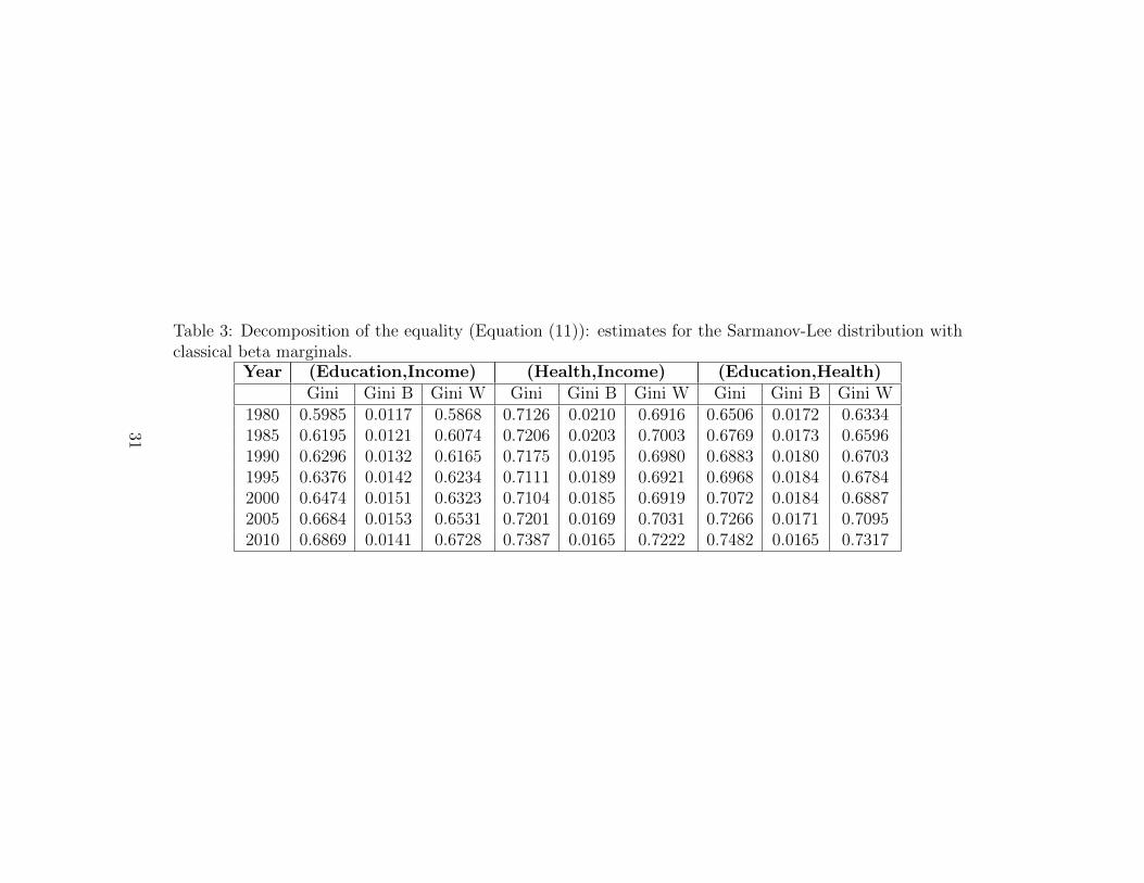
Table 3: Decomposition of the equality (Equation (11)): estimates for the Sarmanov-Lee distribution withclassical beta marginals.
Year (Education,Income) (Health,Income) (Education,Health)Gini Gini B Gini W Gini Gini B Gini W Gini Gini B Gini W
1980 0.5985 0.0117 0.5868 0.7126 0.0210 0.6916 0.6506 0.0172 0.63341985 0.6195 0.0121 0.6074 0.7206 0.0203 0.7003 0.6769 0.0173 0.65961990 0.6296 0.0132 0.6165 0.7175 0.0195 0.6980 0.6883 0.0180 0.67031995 0.6376 0.0142 0.6234 0.7111 0.0189 0.6921 0.6968 0.0184 0.67842000 0.6474 0.0151 0.6323 0.7104 0.0185 0.6919 0.7072 0.0184 0.68872005 0.6684 0.0153 0.6531 0.7201 0.0169 0.7031 0.7266 0.0171 0.70952010 0.6869 0.0141 0.6728 0.7387 0.0165 0.7222 0.7482 0.0165 0.7317
31

References
Arnold, B. C. (1983). Pareto Distributions. International Co-operativePublishing House, Fairland, MD.
Arnold, B.C. (1987). Majorization and the Lorenz Curve, Lecture Notes inStatistics 43, Springer Verlag, New York.
Alkire, S. y Foster, J. (2010). Designing the Inequality-Adjusted HumanDevelopment Index. Human Development Research Paper, 2010/28,PNUD.
Atkinson, A.B. (2003). Multidimensional deprivation: contrasting socialwelfare and counting approaches. Journal of Economic Inequality, 1,51-65.
Atkinson, A.B., Bourguignon, F. (1982). The comparison of multi-dimensioneddistributions of economic status. Review of Economics Studies, 49, 183-201.
Bailey, W. N. (1935). Appell’s Hypergeometric Functions of Two Variables.In: Generalised Hypergeometric Series, Ch. 9. Cambridge UniversityPress: Cambridge, England.
Bairamov, I., Kotz, S. (2003). On a new family of positive quadrant de-pendent bivariate distributions. International Mathematical Journal,3, 1247.1254.
Balakrishnan, N., Lai, C-.D. (2009). Continuous Bivariate Distributions.Springer, New York.
Barro, R., Lee, J.-W. (2010). A New Data Set of Educational Attainment inthe World, 1950-2010. NBER Working Paper 15902, National Bureauof Economic Research, Massachusetts.
Becker, S.G, Philipson, T.J. Soares, R.R. (2005). Quantity and Qualityof Life and the Evolution of World Inequality. American EconomicReview, 95, 277-291.
Bilbao-Ubillos, J. (2011). The limits of Human Development Index: Thecomplementary role of economic and social cohesion, development strate-gies and sustainability. Sustainable Development, DOI: 10.1002/sd.525.
32

0.0
0.5
1.0
pHEducationL
0.0
0.5
1.0
pHIncomeL
0.0
0.5
1.0
qHfHEducatio,IncomeLL
0.0
0.5
1.0
pHHealthL
0.0
0.5
1.0
pHIncomeL
0.0
0.5
1.0
qHfHHealth,IncomeLL
0.0
0.5
1.0
pHhealthL
0.0
0.5
1.0pHEducationL
0.0
0.5
1.0
qHfHHealth,EducationLL
Table 4: Bivariate Lorenz curves: evolution of multidimensional inequality in educationand income (a), health and income (b) and health and education (c) in 1980 (blue) and 2010(green). The curves are defined by Equation (9) with components defined in Equations(15) and (16).
33

Bourguignon, F., Morrison, C. (2002). Inequality among World Citizens.American Economic Review, 92, 727-744.
Briassoulis, H. (2001). Sustainable development and its indicators: Througha (Planner’s) Glass darkly. Journal of Environmental Planning andManagement, 44, 409-427.
Cahill, M.B. (2005). Is the Human Development Index Redundant? EasternEconomic Journal, 31, 12-19.
Chotikapanich, D., Rao, D. S. P., Tang, K. K. (2007). Estimating incomeinequality in China using grouped data and the generalized beta dis-tribution. Review of Income and Wealth, 53, 127-147.
Cornwall, A., Gaventa, J. (2009). From users and choosers to makers andshapers: Repositioning participation in social policy. IDS Bulletin, 31,50-62.
Deaton, A. (2004). Health in Age of Globalization. Brookings Trade Forum2004, Brookings Institution, Washington D.C.
Decancq, K. (2011). Global inequality: A multidimensional perspective.Available at SSRN http://dx.doi.org/10.2139/ssrn.1833253.
Decancq, K., Decoster, A., Schokkaert, E. (2009). Evolution of World In-equality in Well-being. World Development, 37, 11-25.
Decancq, K., Lugo M.A., (2012). Inequality of Wellbeing: A Multidimen-sional Approach. Economica, 79, 721-746.
Duclos, J.-C., Sahn, D., Younger, S. (2006). Robust multidimensionalpoverty comparisons. The Economic Journal, 116, 943-968.
Duclos, J.-C., Sahn, D., Stephen D., Younger, S. (2011). Partial multi-dimensional inequality orderings. Journal of Public Economics, 95,225-238.
Firebaugh, G. (2000). The Trend in Between-Nation Income Inequality.Annual Review of Sociology, 26, 323-339.
Gastwirth, J. L. (1971). A general definition of the Lorenz curve. Econo-metrica, 39, 1037-1039.
34

Goesling, B., Firebaugh, F. (2004). The trend in international health in-equality. Population and Development Review, 30, 131-146.
Grimm, M., Harttgen, K., Klasen, S., Misselhorn, M. (2008). A HumanDevelopment Index by Income Groups. World Development, 36, 2527-2746.
Hicks, D.A. (1997). The Inequality-Adjusted Human Development Index:A Constructive Proposal. World Development, 25, 1283-1298.
Hobin, B., Franses, P.H. (2001). Are living standards converging? Struc-tural Change and Economics Dynamics, 12, 171-200.
Huang, J.S., Kotz, S. (1999). Modifications of the Farlie-Gumbel-Morgensterndistributions. A tough hill to climb. Metrika, 49, 135-145.
Kakwani, N.C. (1977). Applications of Lorenz Curves in Economic Analysis.Econometrica, 45, 719-728.
Kelley, A. (1991). The Human Development Index: “Handle with Care”.Population and Development Review, 17, 315-324.
Kolm, S.C. (1977). Multidimensional Equalitarianisms. Quarterly Journalof Economics, 91, 1-13.
Koshevoy, G. (1995). Multivariate Lorenz majorization. Social Choice andWelfare, 12, 93-102.
Koshevoy, G., Mosler, K. (1996). The Lorenz zonoid of a multivariate dis-tribution. Journal of the American Statistical Association, 91, 873-882.
Koshevoy, G., Mosler, K. (1997). Multivariate Gini indices. Journal ofMultivariate Analysis, 60, 252-276.
Kovacevic, M. (2010). Measurement of Inequality in Human Development-A Review. Human Development Research Paper, 35, PNUD-HDRO,New York.
Lawson-Remer, T., Fukuda-Parr, S., Randolph, S. (2009). An index of eco-nomic and social rights fulfillment: Concept and methodology. Journalof Human Rights, 8, 195-221.
35

Lee, M-L.T. (1996). Properties of the Sarmanov Family of Bivariate Distri-butions, Communications in Statistics, Theory and Methods, 25, 1207-1222.
Maasoumi, E. (1986). The measurement and decomposition of multi-dimensionalinequality. Econometrica, 54, 991-997.
Marshall, A.W., Olkin, I., Arnold, B.C. (2011). Inequalities: Theory ofMajorization and Its Applications. Second Edition. Springer, NewYork.
Martınez, R. (2012). Inequality and the new human development index.Applied Economics Letters, 19, 533-35.
McDonald, J.B. (1984). Some generalized functions for the size distributionof income. Econometrica, 52, 647-663.
McGillivray, M. (1991). The Human Development Index: yet another re-dundant composite development indicator? World Development, 19,1461-1468.
McGillivray, M., Markova, N. (2010). Global Inequality in Wellbeing Di-mensions. Journal Development Studies, 46, 371-378.
McGillivray, M., Pillarisetti, J.R. (2004). International Inequality in Well-Being. Journal of International Development, 16, 563-574.
McGillivray, M., White, H. (1993). Measuring development? The UNDP’sHuman Development Index. Journal of International Development, 5,183-192.
Milanovic, B. (2005). Worlds Apart: Measuring International and GlobalInequality. Princeton University Press, Princeton and Oxford.
Morrison, C., Murtin, F. (2012). The Kuznets curve of human capital in-equality: 18702010. Journal of Economic Inequality, DOI 10.1007/s10888-012-9227-2.
Mosler, K. (2002). Multivariate Dispersion, Central Regions and Depth:The Lift Zonoid Approach. Lecture Notes in Statistics 165, Springer,Berlin.
36

Muller, C., Trannoy, A. (2011). A dominance approach to the appraisalof the distribution of well-being across countries. Journal of PublicEconomics, 95, 239-246.
Neumayer, E. (2001). The Human Development Index and Sustainability -A Constructive Proposal. Ecological Economics, 39, 101-114.
Neumayer, E. (2003). Beyond income: convergence in living standards, bigtime. Structural Change and Economic Dynamics, 14, 275-296.
Noorbakhsh, F. (1998). The Human Development Index: Some TechnicalIssues and Alternative Indices. Journal of International Development,10, 589-605.
Pillarisetti, J.R. (1997). An empirical note on inequality in the world de-velopment indicators. Applied Economic Letters, 4, 145-147.
Pritchett, L. (1997). Divergences, Big Time. Journal of Economic Perspec-tives, 11, 3-17.
Ravallion, M. (1997). Good and Bad Growth: The Human DevelopmentReports. World Development, 25, 631-638.
Sarabia, J.M. (2008). Parametric Lorenz Curves: Models and Applica-tions. In: Modeling Income Distributions and Lorenz Curves. Series:Economic Studies in Inequality, Social Exclusion and Well-Being 4,Chotikapanich, D. (Ed.), 167-190, Springer-Verlag.
Sarabia, J.M., Castillo, E., Pascual, M., Sarabia, M. (2005). Mixture LorenzCurves, Economics Letters, 89, 89-94.
Sarabia, J.M., Castillo, E., Pascual, M., Sarabia, M. (2007). Bivariate In-come Distributions with Lognormal Conditionals. Journal of EconomicInequality, 5, 371-383.
Sarabia, J.M., Castillo, E., Slottje, D. (1999). An Ordered Family of LorenzCurves. Journal of Econometrics, 91, 43-60.
Sarmanov, O.V. (1966). Generalized Normal Correlation and Two-DimensionalFrechet Classes, Doklady (Soviet Mathematics), 168, 596-599.
37
Sen, A. (1988). The Concept of Development, in Chenery H. and Srinivasan,T.N. (eds.), Handbook of Development Economics Elsevier, Amster-dam, vol. I, 9-26.
Sen, A. (1989). Development as Capabilities Expansion. Journal of Devel-opment Planning, 19, 41-58.
Sen, A. (1999). Development as Freedom. Oxford University Press, Oxford.
Seth, S. (2011). A class of distribution and association sensitive multidimen-sional welfare indices. Journal of Economic Inequality, DOI10.1007/s10888-011-9210-3
Slottje, D.J. (1987). Relative Price Changes and Inequality in the Size Dis-tribution of Various Components. Journal of Business and EconomicsStatistics, 5, 19-26.
Srinivasan, T.N. (1994). Human development: a new paradigm or a rein-vention of the wheel? American Economic Review, 84, 238-243.
Taguchi, T. (1972a). On the two-dimensional concentration surface andextensions of concentration coefficient and Pareto distribution to thetwo-dimensional case-I. Annals of the Institute of Statistical Mathemat-ics, 24, 355-382.
Taguchi, T. (1972b). On the two-dimensional concentration surface andextensions of concentration coefficient and Pareto distribution to thetwo-dimensional case-II. Annals of the Institute of Statistical Mathe-matics, 24, 599-619.
Taguchi, T. (1988). On the structure of multivariate concentration - somerelationships among the concentration surface and two variate meandifference and regressions. Computational Statistics and Data Analysis,6, 307-334.
Tsui, K.Y. (1995). Multidimensional generalizations of the relative andabsolute inequality indices: the Atkinson-Kolm-Sen approach. Journalof Economic Theory, 67, 251-265.
Tsui, K.Y. (1999). Multidimensional inequality and multidimensional gen-eralized entropy measures: an axiomatic derivation. Social Choice andWelfare, 16, 145-157.
38

UNDP (2012). International Human Development Indicators. Retrievedfrom http://hdr.undp.org/en/statistics/, last accessed November10, 2012.
World Bank (2001). World Development Report 2000/2001: Attackingpoverty. Oxford and New York, Oxford and New York.
World Bank (2006). World Development Report 2005/2006: Equity andDevelopment. Oxford and New York, Oxford and New York.
39