modeling broadband ocean acoustic transmissions with time

Portland State University Portland State University

PDXScholar PDXScholar

Electrical and Computer Engineering Faculty Publications and Presentations Electrical and Computer Engineering

7-2008

Modeling Broadband Ocean Acoustic Transmissions Modeling Broadband Ocean Acoustic Transmissions

with Time-Varying Sea Surfaces with Time-Varying Sea Surfaces

Martin Siderius Portland State University, [email protected]

Michael B. Porter

Follow this and additional works at: https://pdxscholar.library.pdx.edu/ece_fac

Part of the Electrical and Computer Engineering Commons

Let us know how access to this document benefits you.

Citation Details Citation Details Siderius, M., & Porter, M. B. (2008). Modeling broadband ocean acoustic transmissions with time-varying sea surfaces. Journal of The Acoustical Society of America, 124(1), 137-150.

This Article is brought to you for free and open access. It has been accepted for inclusion in Electrical and Computer Engineering Faculty Publications and Presentations by an authorized administrator of PDXScholar. Please contact us if we can make this document more accessible: [email protected].

https://pdxscholar.library.pdx.edu/

https://pdxscholar.library.pdx.edu/ece_fac

https://pdxscholar.library.pdx.edu/ece_fac

https://pdxscholar.library.pdx.edu/ece

https://pdxscholar.library.pdx.edu/ece_fac?utm_source=pdxscholar.library.pdx.edu%2Fece_fac%2F155&utm_medium=PDF&utm_campaign=PDFCoverPages

http://network.bepress.com/hgg/discipline/266?utm_source=pdxscholar.library.pdx.edu%2Fece_fac%2F155&utm_medium=PDF&utm_campaign=PDFCoverPages

http://library.pdx.edu/services/pdxscholar-services/pdxscholar-feedback/?ref=https://pdxscholar.library.pdx.edu/ece_fac/155

mailto:[email protected]

Modeling broadband ocean acoustic transmissionswith time-varying sea surfaces

Martin Siderius and Michael B. PorterHLS Research Inc., 3366 N. Torrey Pines Ct., Suite 310, La Jolla, California 92037

�Received 2 October 2007; revised 11 April 2008; accepted 15 April 2008�

Solutions to ocean acoustic scattering problems are often formulated in the frequency domain,which implies that the surface is “frozen” in time. This may be reasonable for short duration signalsbut breaks down if the surface changes appreciably over the transmission time. Frequency domainsolutions are also impractical for source-receiver ranges and frequency bands typical forapplications such as acoustic communications �e.g. hundreds to thousands of meters, 1–50 kHzband�. In addition, a driving factor in the performance of certain acoustic systems is the Dopplerspread, which is often introduced from sea-surface movement. The time-varying nature of the seasurface adds complexity and often leads to a statistical description for the variations in receivedsignals. A purely statistical description likely limits the insight that modeling generally provides. Inthis paper, time-domain modeling approaches to the sea-surface scattering problem are described.As a benchmark for comparison, the Helmholtz integral equation is used for solutions to static,time-harmonic rough surface problems. The integral equation approach is not practical fortime-evolving rough surfaces and two alternatives are formulated. The first approach is relativelysimple using ray theory. This is followed with a ray-based formulation of the Helmholtz integralequation with a time-domain Kirchhoff approximation.© 2008 Acoustical Society of America. �DOI: 10.1121/1.2920959�

PACS number�s�: 43.30.Zk, 43.30.Cq, 43.30.Hw, 43.30.Re �SLB� Pages: 137–150

I. INTRODUCTION

For many sonar applications, scattering is treated as aneffective loss mechanism and Doppler shifts are often ig-nored. This may be reasonable for certain types of sonarsystems, particularly the low frequency ones. However, newunderwater acoustic systems, including those for underwateracoustic communications, are sensitive to both scatteringlosses and Doppler. In particular, channel equalizers usedwith bandwidth-efficient, phase-coherent communicationsmethods can be extremely sensitive to Doppler spread. De-signing these equalizers to compensate for Doppler oftenpresents a substantial challenge. Significant Doppler spreadcan be introduced simply from the sound interacting with themoving sea surface; however, the effects are much greaterwhen the source and receiver are also in motion. Simulatingsignals using a physics-based model can greatly aid in thedevelopment of new algorithms and provide valuable perfor-mance predictions. Two simulation methods for signals thatinteract with a time-varying, rough sea surface will be de-scribed in this paper. First, a simple technique is proposedthat includes Doppler effects due to source/receiver and sea-surface motion. This is an extension of an earlier work thatwas developed to simulate active sonar receptions on movingmarine mammals.1 The need for comparisons as well as de-termining the limitations of this approach led to the secondtechnique, which uses an implementation of the time-domainKirchhoff approximation.

This paper is organized as follows. In Sec. II, the Makaiexperiment is described, which is useful in motivating theproblem by presenting measurements of Doppler-sensitivesignals that have interacted with the moving sea surface. In

Secs. III and IV, a ray-based approach is used to model mov-ing sources/receivers as well as a slowly varying sea surface.To model interactions from finer scale sea-surface roughness,Sec. V describes the time-harmonic approach using theHelmholtz–Kirchhoff integral equation. This approach is ex-act for two dimensional problems with a line source. Thissection also provides an implementation of the Kirchhoff ap-proximation, which is numerically much less demandingthan the integral equation. The described methods are devel-oped for line sources but the applications of interest are bet-ter modeled with point sources. Therefore, in Sec. VI, theconversion of line source solutions to point source solutionsis described. Finally, in Sec. VII, the time-domain solution isdeveloped for rough surfaces that move in time by using thetime-domain Kirchhoff approximation.

II. THE MAKAI EXPERIMENT

The motivation for the modeling techniques developedhere can be illustrated with data collected during the Makaiexperiment which took place from September 15 to October1, 2005 near the coast of Kauai, HI.2 The site has a coralsand bottom with a fairly flat bathymetry that was nominally100 m. The water column was variable but typically had amixed layer depth of 40–60 m and was downward refractingbelow. The data were measured on September 24th usingboth stationary and towed sources �from R/V Kilo Moana�.The sources were programmable, underwater acoustic mo-dems developed at SPAWAR Systems Center �referred to asthe Telesonar Testbeds, T1 and T2�.3 Signals were receivedon the AOB array, which is an autonomous system developedat the University of Algarve, Portugal. The AOB is a drifting

J. Acoust. Soc. Am. 124 �1�, July 2008 © 2008 Acoustical Society of America 1370001-4966/2008/124�1�/137/14/$23.00

eight-element self-recording array that resembles the sizeand weight of a standard sonobuoy.4 The experiment geom-etry and bathymetry are shown in Fig. 1. Figure 2 shows aray trace of the T1-AOB acoustic paths. The paths are num-bered on the figure and correspond to �1� direct bounce, �2�surface bounce, �3� bottom bounce, �4� surface-bottombounce, and �5� bottom-surface bounce. The different pathdirections have sensitivity to different velocity components.The higher numbered paths are more Doppler sensitive to thevertical velocity components �e.g., from the moving sea sur-face� and the lower numbered paths �e.g., direct path� aremore sensitive to the horizontal velocity components �e.g.,from the source or receiver motion�.

A binary-phase-shift-keying �BPSK� transmission wasused to analyze the channel.5 This waveform is commonlyused for communication transmissions but for this analysis, itis simply a highly Doppler-sensitive signal that can separatethe multipath in time and Doppler spaces. The transmissionused cycles of a 9.5 kHz sinusoid with phase shifts intro-duced to represent a string of 1’s and 0’s defined by an msequence.5 This signal uses an m sequence �size 1024� with1500 chips /s. The total length of the sequence was 0.682 s.In a static situation, using a matched filter on this waveformproduces an estimate of the channel impulse response. How-ever, in situations with source/receiver and/or sea-surfacemotion, each path can have a different Doppler shift �due tothe angle-dependent propagation paths�. A single Doppler

shift can be applied to the BPSK signal before the matched-filter process. By sweeping over a variety of shifts, the Dop-pler for each received arrival can be estimated. The resultingpicture provides an estimate of the so-called channel scatter-ing function.5 This is referred to as an estimate since a truescattering function requires knowing the continuous timeevolution of the impulse response. This is a difficult mea-surement to make since, in practice, the estimate of the im-pulse response requires time. The described method to esti-mate the scattering function does, however, provide theessential information about the relative arrival times of themultipath and how each is Doppler shifted.

Examples of the processed scattering functions at tworanges from the Makai experiment are shown in Fig. 3. Eachhorizontal trace in the figure results from a matched-filterprocess using different Doppler-shifted replicas denoted s j�t�.The index j corresponds to applied Doppler shifts accordingto the shift factor 1−v j /c, where v j is the assumed speed andc is the reference sound speed. The Doppler replicas, s j�t�,are matched filtered against the received time series.6 That is,

rj�t� = �+�

�

p��s j�� − t�d� , �1�

where p�� is the received time series and rj�� is thematched-filter output. In this way, rj�t� is indexed over timeand Doppler and each multipath arrival produces a peak

FIG. 1. �Color online� Bathymetry near Kauai with the positions of the AOBvertical array and the Telesonar Testbeds T1 and T2 at 01:00 on JD 268. T1was about 600 m away from AOB and being towed while T2 is about2.8 km away and is stationary.

0 100 200 300 400 500 600

0

10

20

30

40

50

60

70

80

90

Range (m)

Dep

th(m

)

1

2

3

5

4

Verticalvelocity

Horizontalvelocity

FIG. 2. Ray trace between testbed T1 and the AOB array. The various pathsare labeled �1� direct, �2� surface bounce, �3� bottom bounce, �4� surface-bottom bounce, and �5� bottom-surface bounce.

Arrival time (s)

Rel

ativ

esp

eed

(m/s

)

0.39 0.4 0.41

1

1.2

1.4

1.6

Arrival time (s)

Rel

ativ

esp

eed

(m/s

)

1.86 1.87 1.88 1.89

−0.5

0

0.5

FIG. 3. �Color online� Left panel shows the measuredimpulse response �or scattering function� for variousDoppler shifts indicated on the y axis �as relative speedin m/s� between the drifting AOB and the stationary T2at 01:04 on JD 268. Each bright spot corresponds to anarrival with delay time shown along the x axis. Rightpanel is for a reception from the towed source T1 at01:02 on JD 268.

138 J. Acoust. Soc. Am., Vol. 124, No. 1, July 2008 M. Siderius and M. B. Porter: Modeling in time-varying channels

when the Doppler shift of the replica is matched with thatarrival.

In the left panel of Fig. 3, the measured scattering func-tion is shown for a 2.8 km range separation between thefixed Testbed T2 and the drifting AOB. The second measuredscattering function is shown in the right panel and is from thetowed Testbed T1 and received on the AOB about 600 maway. The bright spots indicate an arrival in time �i.e., delaytime� along the x axis. Note that only the relative time isknown so the time series are aligned based on the first arrivaland the known distance between the source and receiver. They axis shows the relative speed �i.e., Doppler� that corre-sponds to the peaks. The left panel had the stationary sourceand the Doppler indicates that the AOB was drifting at about0.1–0.2 m /s. The estimate from GPS positions indicatedabout 0.12 m /s. The first arrivals show decreasing Dopplerfollowed by the last visible arrival having an increased Dop-pler shift. For horizontal velocity one expects the later arriv-als to have decreasing Doppler shifts due to higher propaga-tion angles relative to the direction of motion. The highDoppler on the last arrival implies a component in the verti-cal which would introduce larger shifts for late arrivals. Theright panel of Fig. 3 shows the reception from T1 which wasbeing towed with relative speed between T1 and the AOB ofabout 1.2–1.4 m /s. The estimate from GPS positions is1.24 m /s. Like the stationary case, Doppler shifts do notdecrease monotonically on the steeper paths but, in somecases, increase. The paths can be identified using the raytrace in Fig. 1. The second and fourth arrivals both haveincreased Doppler shifts relative to the direct path while thethird arrival has a slightly decreased Doppler. Paths 2 and 4correspond to the surface and surface-bottom bounce pathswhile the third arrival is the bottom bounce. Note that in bothfigures, only the first few paths are visible; the later arrivalsare more attenuated due to surface/bottom interactions.

In the context of acoustic communications, the spreadfactor is often used to determine the type of channel andtherefore the signaling waveforms. The spread factor is de-fined as TmBd where Tm is the multipath time duration �s� andBd is the Doppler spread �Hz�. If the spread factor is less than1, the channel is said to be underspread, and if it is greaterthan 1 it is overspread. It can be highly useful to model theeffects that influence the channel spread as this can lead toacoustic communication improvements as well as perfor-mance prediction. While the spread factor is a simple metric,it does not give a complete description. For example, doesthe multipath consist of many arrivals or just a few? Theinformation given in Fig. 3 show not only the multipath de-lay and Doppler spread but also show the total number andstrength of the arrivals. In this example, the spread factor isrelatively large but the total number of arrivals is small �i.e.,sparse channel�. All of these factors are important for com-munications and correct modeling of these is the primarygoal of this work. Modeling techniques that can be applied inestimating the multipath delay and Doppler spread are thetopic of the next sections.

III. MODELING SOURCE AND RECEIVER MOTIONWITH RAYS

In this section, a relatively simple implementation oftwo dimensional ray methods is extended to treat movingreceivers and a moving sea surface. The goals are somewhatsimilar to the work of Keiffer et al.7 but the approach isdifferent, and the emphasis is on broadband signals for ap-plication to underwater communications, for example. In aray formulation, the complex pressure field, P��, can berepresented as a sum of N arrival amplitudes An�� and de-lays �n�� according to

P�� = S��n=1

N

Anei��n, �2�

where S�� is the spectrum of the source. The specifics ofthe ray trace algorithm are not critical and there are a numberof ray trace models that could have been used here. A sum-mary of most of these type of models can be found fromEtter8 and Jensen et al.9 In the cases considered here, anazimuthally symmetric geometry is assumed and the arrivalamplitudes and delays are computed using the two dimen-sional Gaussian beam implementation in the Bellhoppackage.10,11

According to the convolution theorem, a product of twospectra is a convolution in the time domain. This leads to thecorresponding time-domain representation for the receivedwaveform, p�t�, which is often written as

p�t� = �n=1

N

An�t�s�t − �n�t�� , �3�

where s�t� is the source waveform. This expression showshow the sound is represented as a sum of echoes of thetransmission with associated amplitudes and delays. A timedependency has been introduced in the amplitudes and de-lays to allow the channel to be time varying. The time varia-tions can be caused by many factors including source/receiver motion or sea-surface changes.

The situation is a bit more complicated because the am-plitudes in Eq. �3� are actually complex numbers. This isdue, for example, to bottom reflections that introduce a phaseshift �e.g., a � /2 phase shift�. Since this is a constant phaseshift over frequency, it does not simply introduce an addi-tional time delay. Therefore, a more careful application ofthe convolution theorem is required:

p�t� = �n=1

N

Re�An�t��s�t − �n�t�� − Im�An�t��s+�t − �n�t�� ,

�4�

where s+=H�s� is the Hilbert transform of s�t�. The Hilberttransform is a 90° phase shift of s�t� and accounts for theimaginary part of An. An interpretation of Eq. �4� is that anyarbitrary phase change is treated as a weighted sum of theoriginal waveform and its 90° phase-shifted version. Theweighting controls the effective phase shift.

One of the goals of this work is to simulate the receivedfield in cases where the receiver and/or sea surface is in

J. Acoust. Soc. Am., Vol. 124, No. 1, July 2008 M. Siderius and M. B. Porter: Modeling in time-varying channels 139

motion. In those cases, the arrival amplitudes and delays inEq. �3� change continuously in time. Therefore, new valuesfor An and �n are required at each time step of the signaltransmission. In theory, at each time step, a new set of arrivalamplitudes and delays could be computed with an entirelynew ray trace from the source to the exact receiver locationat that particular time step. However, this would be compu-tationally expensive and mostly unnecessary since thechanges �in amplitude and delay� are likely to be very smallbetween time steps. Alternatively, the ray amplitudes and de-lays are computed on a relatively sparse grid of points inrange and depth. The ray information at any given locationand time is computed through interpolation. The interpola-tion scheme is critical to avoid glitches in the final timeseries that might be caused by jumping too suddenly betweenpoints in the computational grid.

The interpolation of ray amplitudes and delays may ap-pear simple enough but there are some subtleties which cancause difficulties. Consider four neighboring grid points asshown in Fig. 4 where at some particular time step, the re-ceiver is located somewhere inside those points. The moststraightforward way one might think to calculate the field atthis interior point is to identify the same arrival on each ofthe four corners and then interpolate that arrival amplitudeand delay from the four grid points to the receiver location.A problem with that approach occurs when arrival patternson one grid point do not correspond to those at another. Thatis, reflections and refraction effects can cause a differentnumber of rays and different ray types on each of the gridpoints. For example, consider a direct arrival on one cornerof the grid that is refracted away from another grid point. Inthis case, interpolating between these grid points for thatarrival number may involve interpolation of a direct pathwith a bottom bounce path and this will produce incorrectresults.

One could keep careful track of all rays and ray types toensure proper interpolation but that can lead to excessivebookkeeping and storage. Instead, a different interpolationapproach is used here. The amplitudes at the four grid pointsare maintained as separate quantities and their correspondingdelays are adjusted by the ray path travel time differencesbetween the corners of the computational grid and the pointof the receiver �x ,y�. The geometry is shown in Fig. 4 with

an arrival indicated as a dashed line traveling at angle � atthe lower left grid point. The delay time for that arrival isadjusted from position �x1 ,y1� to position �x ,y� by the dis-tance divided by sound speed,

�delay = ��x cos � + �y sin ��/c , �5�

where, for example, �x=x−x1 is positive �increased delay�for position 1.

The contribution of the arrivals from each of the gridpoints is weighted according to

�1 − w1� � �1 − w2� � a1,

�1 − w1� � w2 � a2,

�6�w1 � w2 � a3,

w1 � �1 − w2� � a4,

where a1, a2, a3, and a4 represent the arrival amplitudes ateach corner and the weights are

w1 = �x − x1�/�x2 − x1� ,

�7�w2 = �y − y1�/�y2 − y1� .

Thus, w1 represents a proportional distance in the x directionand w2 represents a proportional distance in the y direction.To summarize, the received field is constructed using Eq. �4�with an additional sum over each of the four corners�weighted amplitudes�.

A. Test cases for source/receiver motion

The previous section presented the method and here, afew examples are given to illustrate the model at low andhigh frequencies. The first example will illustrate the qualityof the ray interpolation. A tone is transmitted at 350 Hz froma source at a depth of 30 m �i.e., continuous wave or �cw��.The environment has a linearly decreasing sound speed thatis 1500 m /s at the surface and 1490 m /s at the seabed at100 m depth. The seabed has a compressional sound speedof 1600 m /s, density of 1.5 g /cm3, and attenuation of0.1 dB /� �decibels per wavelength�. In Fig. 5 is a static fre-quency domain solution for the transmission loss �TL� out to

Point at (x, y)

Amplitude a1 at (x1, y1)




∆x

∆y

θ

FIG. 4. Four points of the computational grid for a raytrace. The actual arrivals are computed at the four cor-ners and any point in the interior computed throughinterpolation of the amplitudes and extrapolation of thedelays. A sample arrival is shown traveling at angle �.


5 km in range �i.e., a standard TL calculation�.9 Next, thetime-series simulator records the pressure field on a receiverthat sweeps out the same 5 km range in time. By using 100of these receivers placed at 1 m increments in depth, theentire range-depth volume is swept out over 100 s �each re-ceiver moves from 0 to 5 km over 100 s�. The amplitude ofthese time-series data are plotted on a decibel scale in Fig. 6.For this simulation, a single ray trace computed the arrivalamplitudes and delays at each point in a grid of 1 m in depthand 100 m in range. Each moving receiver was placed atdepths in between these grid points to ensure all computedvalues were from interpolation rather than exactly falling ongrid points. Even for the relatively large grid spacing, thetechnique produces a good result when compared to the cwTL in Fig. 5.

The second example is for a higher frequency transmis-sion at 10 kHz and illustrates the interpolation as well as theDoppler effects. The environment is the same as for the first

example, but a slightly denser grid is used for the ray calcu-lation due to the higher frequency �0.5 m depth spacing and50 m range spacing�. This is still around three wavelengthsin depth and several hundred wavelengths in range betweengrid points. A single line of pressure amplitude is shown inthe upper panel of Fig. 7 at a receiver depth of 50.25 m�between grid points� and is compared to the cw calculation.The moving receiver speed is 10 m /s and this introduces aDoppler shift of around 67 Hz �moving away from thesource horizontally�. From the agreement in the pressure am-plitudes �between static and moving�, one might incorrectlyassume that the Doppler effects are of little importance.However, various acoustic systems may be significantly im-pacted by Doppler. For example, the spectrum of the re-ceived time series is shown in the lower panel of Fig. 7. Thespectrum shows the direct path shifted by the expected67 Hz as well as a set of less Doppler-shifted peaks due tothe multipath that travels more vertically than the direct path.This type of Doppler spread is one of the primary mecha-nism that cause channel equalizers to fail in coherent com-munication schemes �i.e., coherent acoustic modems�.

IV. MODELING TIME-VARYING SEA SURFACES

The previous section only considered the motion of thereceiver. This could also approximate the solution for thecase when both source and receiver are moving horizontally�possibly at different speeds� in a range independent environ-ment. A time-varying sea surface can be added to the model�with receiver motion only� with slight modifications. In thiscase, the sea surface is assumed to vary slowly in range asmight be the case for swell, ignoring small scale roughness.This limitation will be explored further in the next sectionswhen the rough, time-varying surfaces are considered. Tomodify the previously described algorithm, additional raytraces are computed to sample the time-evolving sea surface.Figure 8 diagrams the required interpolation scheme to in-

Range (km))

Dep

th(m

)

1 2 3 4 5

0

10

20

30

40

50

60

70

80

90

100 20

30

40

50

60

70

80

FIG. 5. �Color online� Frequency domain �350 Hz� TL calculation �dB� overrange and depth with the source at a depth of 30 m.

Time (s)

Dep

th(m

)

0 20 40 60 80

0

10

20

30

40

50

60

70

80

90

100 20

30

40

50

60

70

80

FIG. 6. �Color online� Same as Fig. 5 except calculated using the time-domain approach. That is, a set of moving receivers sweep out �in time� theacoustic TL. Note the different x axes between this figure and Fig. 5. At thislow frequency, the Doppler shift is not significant enough to noticeablychange the TL.

1.9 1.92 1.94 1.96 1.98 20

10

20

30

40

Pre

ssur

eam

plitu

de

Range (km)

10 kHz Time−seriesCW

0 2 4 6 8 10

Time (s)

9925 9930 9935 9940 99450

20

40

60

80

100

120

Pre

ssur

eam

plitu

de

Frequency (Hz)

FIG. 7. �Color online� Top panel shows the cw solution vs range and thetime-series solution vs time as the receiver moves out in range. The corre-sponding range and time x axes are indicated. The lower panel shows thespectrum of the time-series solution with the Doppler shifts which differ forthe various paths.


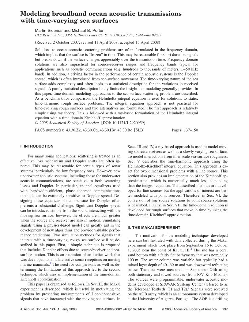
clude surface motion. At an initial time, t= ta, the surface canhave an arbitrary shape and this evolves in time to produce asurface shape defined at time t= tb. The time interval tosample the surface adequately is on the order of the timeinterval of the swell being modeled. This is typically muchless than the sampling interval for the acoustic transmission.Therefore, ray arrival amplitudes and delays are computedfor surfaces at t= ta and t= tb and trilinear interpolation isused in much the same way as described previously withbilinear interpolation. One difference is that the delays arenot extrapolated for this third dimension. The proper arrivalamplitudes and delays are simply determined through theweights applied to the eight corners of the computation grid.As with the previous two dimensions, the arrivals are kept asseparate quantities on each of the eight corners of the cubedepicted in Fig. 8. The delays at each corner of the cube areadvanced or retarded according to distance and the weightgiven to each corner is determined by

�1 − w1� � �1 − w2� � �1 − w3� � a1,

�1 − w1� � w2 � �1 − w3� � a2,

w1 � w2 � �1 − w3� � a3,

w1 � �1 − w2� � �1 − w3� � a4,

�8��1 − w1� � �1 − w2� � w3 � b1,

�1 − w1� � w2 � w3 � b2,

w1 � w2 � w3 � b3,

w1 � �1 − w2� � w3 � b4,

where a1, a2, a3, and a4 represent the arrival amplitudes ateach corner at t= ta and b1, b2, b3, and b4 represent the arrivalamplitudes at each corner at t= tb. The weights are

w1 = �x − x1�/�x2 − x1� ,

w2 = �y − y1�/�y2 − y1� ,

�9�w3 = �t − ta�/�tb − ta� .

The time steps, ta and tb, where the ray traces are computed,are typically at time intervals much greater than the acousticsampling time interval. Therefore, many of the time stepsrely on interpolated arrival information.

A. Test cases for source/receiver motion with a time-varying sea surface

To check the developed algorithm, a comparison can bemade between results using the approach outlined in the pre-vious sections with an exact solution. The exact solution re-quires the water column to be isospeed and the sea surface tobe flat but can vary in height over time �i.e., a flat surfacethat can move up and down�. This is a reasonable compari-son since the approach outlined using a ray tracing algorithmis the same whether the sound speed is depth dependent �ornot� and regardless of the shape of the surface.

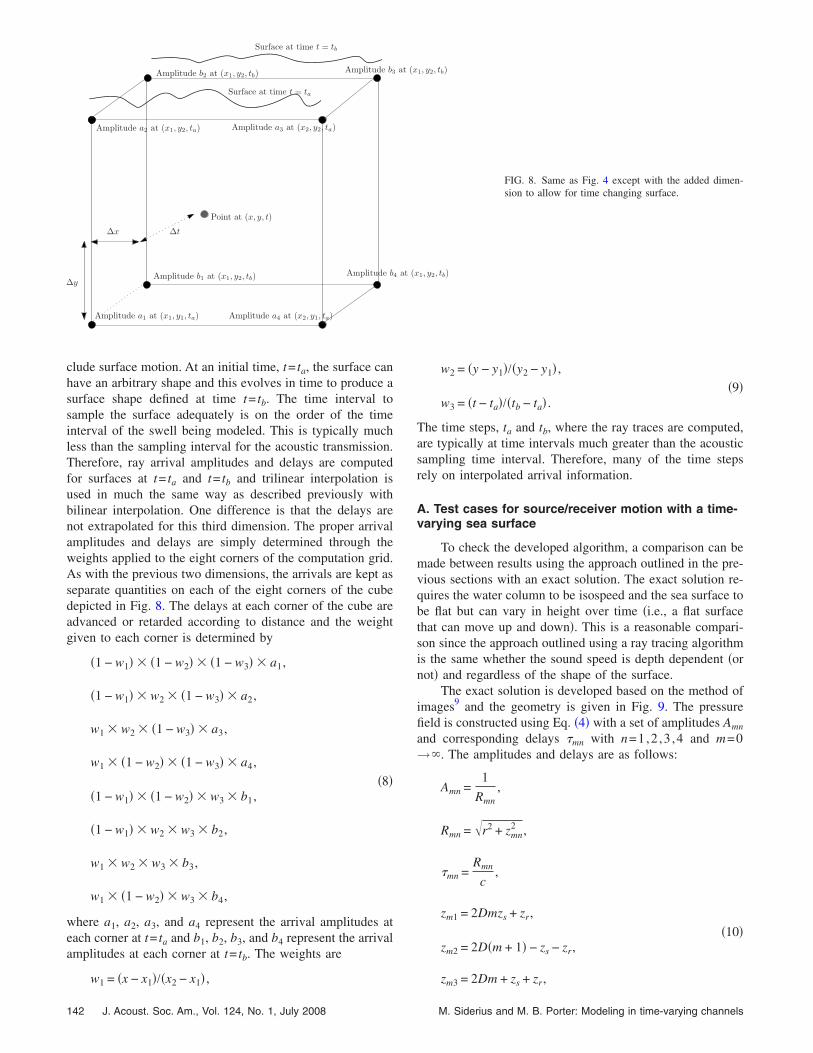
The exact solution is developed based on the method ofimages9 and the geometry is given in Fig. 9. The pressurefield is constructed using Eq. �4� with a set of amplitudes Amn

and corresponding delays �mn with n=1,2 ,3 ,4 and m=0→�. The amplitudes and delays are as follows:

Amn =1

Rmn,

Rmn = �r2 + zmn2 ,

�mn =Rmn

c,

zm1 = 2Dmzs + zr,

�10�zm2 = 2D�m + 1� − zs − zr,

zm3 = 2Dm + zs + zr,

Point at (x, y, t)

Amplitude a1 at (x1, y1, ta)




∆x

∆y

∆t

Surface at time t = ta

Surface at time t = tb

Amplitude b2 at (x1, y2, tb) Amplitude b3 at (x1, y2, tb)

Amplitude b4 at (x1, y2, tb)Amplitude b1 at (x1, y2, tb)

FIG. 8. Same as Fig. 4 except with the added dimen-sion to allow for time changing surface.


zm4 = 2D�m + 1� + zs − zr,

where zs is the source depth, zr is the receiver depth, r is thereceiver range, D is the water depth, and c is the water soundspeed �isospeed at 1500 m /s�. The one twist in this standardformulation is that the surface is moving in time, whichcauses the amplitudes and delays to vary in time. The varia-tions in the surface are incorporated into the terms of Eq.�10� through adding a time dependence to D, zs, and zr sincethe effective water depth and the source and receiver depthschange with time. By making use of Eq. �4� with these time-dependent amplitudes and delays, the exact received timeseries can be determined.

To illustrate the comparison, consider an example withD=100 m, zs=30 m, zr=40 m, and r=250 m. The receiveris moving toward the source at 0.75 m /s. The sea surface ismoving away from the seabed at a speed of 0.25 m /s. In thisway, the Doppler shifts for surface interacting paths will bereduced from 0.75 m /s. The waveform chosen for this ex-ample is extremely Doppler sensitive such that the multipath�each having distinct Doppler shifts� can be separated in bothdelay time and Doppler space. The transmission waveformused is the BPSK signal that was used in the Makai experi-ment. The separation between grid points �as in the cubeshown in Fig. 8� are as follows: the depth spacing was 1 m,the range spacing was 5 m, and the distance between sur-faces was 0.0125 m; this implies a new surface every12.5 ms �i.e., 40 ray traces were computed for surface per-turbations between 0 and 0.5 m�.

The results are shown in Fig. 10. In panel �a� of thefigure is the exact impulse response shown in delay and Dop-pler space �i.e., the “scattering function”�. In panel �b� of Fig.10 is the arrival structure using the time-dependent ray inter-polation algorithm previously described. In �a� and �b�, thefirst path is the direct one and has a Doppler shift corre-sponding to −0.75 m /s due to the horizontal receiver motion�directly toward the source�. The next path is due to thesurface bounce and is less Doppler shifted due to the sea-surface motion acting to Doppler shift in the opposite direc-

tion. The next path is the bottom bounce and this path isunaffected by the surface motion and is Doppler shifted lessthan the direct path due to the more vertical directionality ofthe ray path. The next arrivals are due to multiple bottom-surface bounces.

V. MODELING STATIC, ROUGH SEA SURFACES

The previous section developed a method for modelingtime series with gently varying sea surfaces like that fromswell and the next sections provide an alternative formula-tion which is more appropriate for finer scale roughness.Rough surface scattering has been extensively studied andthere is a huge amount of literature on the subject �see, forexample, the text by Ogilvy�.12 To begin, exact solutions forone-dimensional static rough surfaces are described by usingthe Helmholtz integral equation. This will be compared tosolutions found with a ray trace solution �e.g., Bellhop� withsurface roughness. This will be further developed with theuse of the Kirchhoff approximation to yield a time-domainversion for scattering from rough, time-evolving surfaces.

A. Helmholtz integral equation

The description in this section will follow the notationand derivation from Thorsos.13 Those results are presentedfor completeness and to establish the notation being used.The exact solution to the time-harmonic �e−i�t� one-dimensional sea surface �free surface boundary� is given bythe Helmholtz integral equation,

p�r� = pinc�r� −1

4i�

S

H0�1��k�r − r��

�p�r��n�

ds�. �11�

That is, the total field is a sum of the incident and scatteredfields, p�r�= pinc�r�+ pscat�r�. In Eq. �11�, the acoustic wave

2D + zs

2D − zs

−zs

zs

zr

R03

R01

R02

R04

D

z

r

FIG. 9. Geometry showing the location and ranges of the source, receiver,and corresponding images.

Spe

ed(m

/s)

Multipath amplitude (dB)

(a)

−1

−0.5

0

0.5 −8

−6

−4

−2

0

Time delay (s)

Spe

ed(m

/s)

(b)

0.16 0.18 0.2 0.22 0.24 0.26 0.28 0.3

−1

−0.5

0

0.5 −8

−6

−4

−2

0

FIG. 10. �Color online� In panel �a�, the exact impulse response �normal-ized� is computed using the method of images and in �b�, it is computedusing the time-dependent ray interpolation method described. The first ar-rival in time is from the direct path and shows only a Doppler shift due tothe receiver horizontal motion of −0.75 m /s. The next two paths that followare from the surface and bottom bounces. The additional multipaths are dueto multiple interactions with the sea surface and the bottom.


number is given by k=� /c, the quantity �p�r�� /�n� is thenormal derivative of the pressure field on the surface, andH0

�1� is the zero-order Hankel function of the first kind. Onthe surface the pressure field is zero, such that

pinc�r� =1

4i�

S

H0�1��k�r − r��

�p�r��n�

ds�. �12�

The quantity of interest is the total pressure field p�r� whichrequires first solving Eq. �12� for �p�r�� /�n�.

Equation �12� can be approximately solved by using nu-merical integration,

am = �n=1

N

Amnbn, m = 1, . . . ,N , �13�

where am is the incident field, and Amn are the Hankel func-tions,

am = pinc�rm� ,

�14�

Amn = H0�1��k�rm − rn�� if m � n

H0�1��k�x/2e�m� if m = n ,

and

bn = ��x

4in

�p�r��n�

� rn

. �15�

The surface height function is defined as f�x� with 2�x��=1+ �df�x�� /dx��2 and ds�=�x��dx�. Using unit vectors xand z, the vector r is defined as rm=xmx+ f�xm�z and xm

= �m−1��x−L /2, with m=�xm� and L being the totallength of the surface.

By using matrix notation, Eq. �13� can be written as

a = Ab , �16�

with solution for b determined through inversion of A,

b = A−1a . �17�

Once this equation is solved for b, the scattered field is ob-tained by using

pscat�r� = �n=1

N

H0�1��k�rm − rn��bn. �18�

The practical limitations of numerically solving theseequations is the inversion of matrix A. In practice, the sam-pling of the surface requires approximately five points perwavelength. To keep from introducing artifacts, the compu-tational domain has to be even larger than the region of in-

terest �here, it was extended by 250 m�. If the objective is tosolve a problem with a 1 km surface at 10 kHz �for example,for an acoustic communication simulation�, the number ofdiscrete points is over 30 000, which requires inversion of a30 000�30 000 matrix for each frequency. This increases to300 000�300 000 for a 10 km simulation. Add to this therequirement that this be done over a broad band of frequen-cies for many practical problems, and it becomes even moredifficult. To make matters worse, if the objective is to deter-mine the time-evolving nature of the scattering, this must bedone at many time steps. The size of the problem by usingexact solutions becomes apparent and leads to the approxi-mations used in the next sections. The exact approach out-lined here is valuable, however, to provide ground-truthcomparison with the approximate methods.

B. Ray approach with the Kirchhoff approximation

The Kirchhoff approximation is as follows:

�p�r��n

� 2�pinc�r�

�n. �19�

The value of this approximation is that the elements of bn

required for the scattered field are no longer dependent onthe total field but only on the incident field. This removes theneed to store and invert the matrix A. Another way to thinkabout the solution for the scattered field is that the surface isremoved and replaced by point sources at each discrete lo-cation xn. The weight of each point source is determined bythe coefficients bn. This is basically a statement of the Huy-gens principle14 and is depicted in Fig. 11. For the exactsolution, each point source amplitude bn depends on each ofthe others, while for the Kirchhoff approximation, it is only alocal reflection. However, the Huygens sources can reradiatein all directions and the dense sampling allows for a morecomplicated scattered field than that from a specularly re-flected ray trace.

The incident field can be written in terms of a ray am-plitude and delay �far field approximation for the HankelFunction� from the source to each of the Huygens secondarysources,

pinc�rn� �1

�kR1n

ei��1n, �20�

where R1n and �1n are computed similarly to Eq. �10� for the01 path for the surface bounce �suppressing the first indexwhich is unnecessary here since there are no higher orderimages�. Since the Huygens reconstruction removes the sur-

� � � � � � � � ��

Source

Receiver

b1 b2bN

bN−1

Surface

FIG. 11. Diagram illustrating the surface is replaced bya set of Huygens sources.


face boundary and replaces it with secondary sources, theonly other path to arrive in the incident field is from thebottom bounce path 02. The total incident field at each Huy-gens secondary source has two terms,

pinc�rn� =ei��1n

�kR1n

+Vnei��2n

�kR2n

, �21�

where the second term has been modified to include the bot-tom loss Vn that occurs for a nonpressure release bottom.This term will generally be a function of the angle incidenton the bottom and is therefore indexed to each point on thesurface. Further, this assumes a plane wave reflection losswhich is a slight approximation. The expression for the inci-dent field has been written out for this isospeed case forclarity; however, these two terms can be easily taken from aray trace algorithm that would include refraction for morerealistic cases. The weights for the Huygens secondarysources are computed using Eq. �15� and taking the deriva-tive of pinc�rn�,

bn � kNn ei��1n

�kR1n

+Vnei��2n

�kR2n� , �22�

where

Nn =e−i�/4�xn

�2��sr,n cos �n + sz,n sin �n� , �23�

with sr,n sz,n the unit vector components for the normal to the

surface at rn and � the direction of propagation of pinc. The Nand k in Eq. �22� appear due to the derivative in the directionnormal to the surface. The value of bn is an approximation tothe derivative since the higher order terms of the derivativeare neglected �i.e., the terms with R−3/2�.

For the general cases considered here, there is a seabedboundary so the free-space Hankel function is replaced inEq. �11� with the Green’s function G�k�r− r�� representingthe point source response between r and r�.

p�r� = pinc�r� −1

4i�

S

G�k�r − r��p�r��

�n�ds�. �24�

For the numerical implementation, the Green’s function has asimilar form as the incident field,

G��r − rn�� =ei�r1n

�kR1n

+Vnei��2n

�kR2n

, �25�

where in this case, R1n represents the distance for the directpath between the Huygens secondary source �at rn� and the

field point �at r� and R2n, represents the distance for thebottom bounce path.

The scattered field is then constructed as


N

G�k�r − rn��bn, �26�

where the total scattered field is a sum of four componentsfor each Huygens source,


N

�m=1

4

Nn�Amei�Tm� , �27�

with the amplitudes

A1 =1

R1nR1n

,

A2 =Vn

R2nR1n

,

�28�

A3 =Vn

R1nR2n

,

A4 =Vn

2

R2nR2n

,

and the delays

T1 = �1n + �1n,

T2 = �2n + �1n,

�29�T3 = �1n + �2n,

T4 = �2n + �2n.

The frequency dependent k term conveniently cancels out.However, this is a line source formulation and this frequencydependence will become necessary when extending to apoint source, which is required for typical applications. Thisissue will be discussed further in Sec. VI. It is also worthnoting that this formulation includes one surface bouncepath. That is, the total field will consist of a direct path,bottom-bounce, bottom-surface-bounce, surface-bottom-bounce, and bottom-surface-bottom-bounce paths. For manyapplications, these six paths will provide a sufficient impulseresponse representation. However, paths with multiple sur-face bounces could be included in an approximate way bymodifying the amplitude of the first surface bounce by takingonly the specular path and then include the scattering in thesecond interaction with the surface.

C. Examples of scattering approaches for staticsurfaces

Static surfaces at a single frequency are useful forchecking the approximate solutions since the exactHelmholtz–Kirchhoff integral equation can be used as theground truth. The time-domain Kirchhoff approach will notimmediately show its utility for these time-harmonic ex-amples. However, that formulation will be critical when ex-tending to the time-varying surfaces in Sec. VII.

1. Surface scattering without a seabed

In the first example, the field interactions with the roughsea surface is determined without a seabed. Using an isos-peed water column allows the exact Hankel functions to be


included in the Helmholtz–Kirchhoff integral equation. Thesource depth was 40 m from the surface and the frequencywas 200 Hz.

To generate the random surface shape, a spectral methodwas used similar to that by Thorsos.13 That is, white noise isfiltered with a Gaussian spectrum to provide a one-dimensional random sequence with height and correlationdistance governed by the parameters of the Gaussian density,its mean, and correlation. For the first example, the surfaceheight standard deviation is 0.5� and the correlation length is50�.

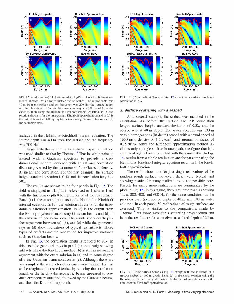
The results are shown in the four panels in Fig. 12. Thefield is displayed as TL �TL is referenced to 1 Pa at 1 m�with the line near depth 0 being the shape of the sea surface.Panel �a� is the exact solution using the Helmholtz–Kirchhoffintegral equation. In �b�, the solution shown is for the time-domain Kirchhoff approximation. In �c� is the output fromthe Bellhop ray/beam trace using Gaussian beams and �d� isthe same using geometric rays. The results show nearly per-fect agreement between �a�, �b�, and �c� while the geometricrays in �d� show indications of typical ray artifacts. Thesetypes of artifacts are the motivation for improved methodssuch as Gaussian beams.

In Fig. 13, the correlation length is reduced to 20�. Inthis case, the geometric rays in panel �d� are clearly showingartifacts while the Kirchhoff method �b� is still in reasonableagreement with the exact solution in �a� and to some degreealso the Gaussian beam solution in �c�. Although these arejust samples, the results for other cases were similar. That is,as the roughness increased �either by reducing the correlationlength or the height� the geometric beams appeared to pro-duce erroneous results first, followed by the Gaussian beams,and then the Kirchhoff approach.

2. Surface scattering with a seabed

As a second example, the seabed was included in thecalculation. As before, the surface had 20� correlationlength, surface height standard deviation of 0.5�, and thesource was at 40 m depth. The water column was 100 mwith a homogeneous �in depth� seabed with a sound speed of1600 m /s, density of 1.5 g /cm3, and attenuation factor of0.75 dB /�. Since the Kirchhoff approximation method in-cludes only a single surface bounce path, the figure that it iscompared against was computed with the same paths. In Fig.14, results from a single realization are shown comparing theHelmholtz–Kirchhoff integral equation result with the Kirch-hoff approximation.

The results shown are for just single realizations of therandom rough surface; however, these were typical andshowing results for many realizations is not possible here.Results for many more realizations are summarized by theplots in Fig. 15. In this figure, there are three panels showingTL at 200, 400, and 600 Hz for the same conditions as theprevious case �i.e., source depth of 40 m and 100 m watercolumn�. In each panel, 50 realizations of rough surfaces areaveraged. This is similar to the comparisons made byThorsos13 but those were for a scattering cross section andhere the results are for a receiver at a fixed depth of 25 m.

FIG. 12. �Color online� TL �referenced to 1 Pa at 1 m� for different nu-merical methods with a rough surface and no seabed. The source depth was40 m from the surface and the frequency was 200 Hz, the surface heightstandard deviation is 0.5� and the correlation length is 50�. Panel �a� is theexact solution using the Helmholtz-Kirchhoff integral equation, in �b� thesolution shown is for the time-domain Kirchhoff approximation and in �c� isthe output from the Bellhop ray/beam trace using Gaussian beams and �d�for geometric rays.

FIG. 13. �Color online� Same as Fig. 12 except with surface roughnesscorrelation is 20�.

FIG. 14. �Color online� Same as Fig. 13 except with the inclusion of asmooth seabed at 100 m depth. Panel �a� is the exact solution using theHelmholtz–Kirchhoff integral equation. In �b�, the solution shown is for thetime-domain Kirchhoff approximation.


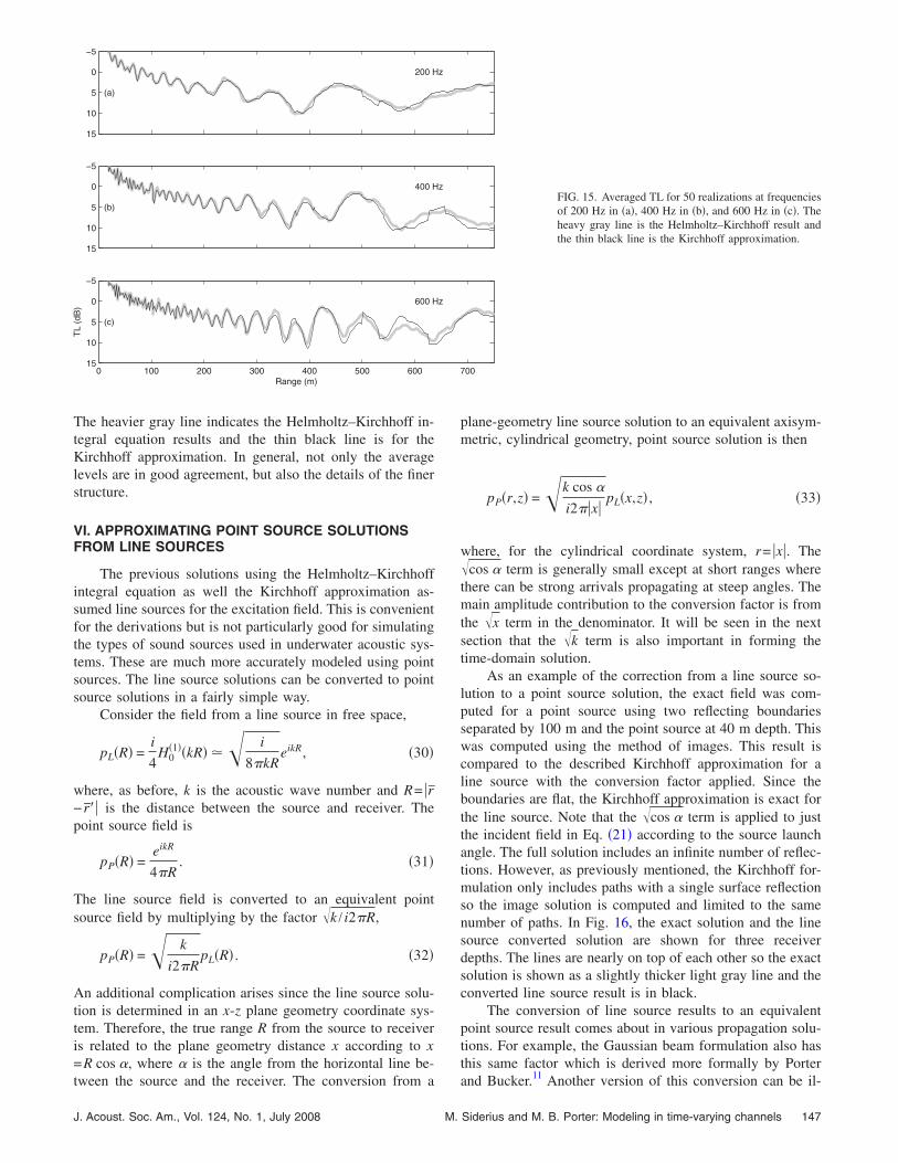
The heavier gray line indicates the Helmholtz–Kirchhoff in-tegral equation results and the thin black line is for theKirchhoff approximation. In general, not only the averagelevels are in good agreement, but also the details of the finerstructure.

VI. APPROXIMATING POINT SOURCE SOLUTIONSFROM LINE SOURCES

The previous solutions using the Helmholtz–Kirchhoffintegral equation as well the Kirchhoff approximation as-sumed line sources for the excitation field. This is convenientfor the derivations but is not particularly good for simulatingthe types of sound sources used in underwater acoustic sys-tems. These are much more accurately modeled using pointsources. The line source solutions can be converted to pointsource solutions in a fairly simple way.

Consider the field from a line source in free space,

pL�R� =i

4H0

�1��kR� �� i

8�kReikR, �30�

where, as before, k is the acoustic wave number and R= �r− r�� is the distance between the source and receiver. Thepoint source field is

pP�R� =eikR

4�R. �31�

The line source field is converted to an equivalent pointsource field by multiplying by the factor �k / i2�R,

pP�R� =� k

i2�RpL�R� . �32�

An additional complication arises since the line source solu-tion is determined in an x-z plane geometry coordinate sys-tem. Therefore, the true range R from the source to receiveris related to the plane geometry distance x according to x=R cos �, where � is the angle from the horizontal line be-tween the source and the receiver. The conversion from a

plane-geometry line source solution to an equivalent axisym-metric, cylindrical geometry, point source solution is then

pP�r,z� =�k cos �

i2��x�pL�x,z� , �33�

where, for the cylindrical coordinate system, r= �x�. The�cos � term is generally small except at short ranges wherethere can be strong arrivals propagating at steep angles. Themain amplitude contribution to the conversion factor is fromthe �x term in the denominator. It will be seen in the nextsection that the �k term is also important in forming thetime-domain solution.

As an example of the correction from a line source so-lution to a point source solution, the exact field was com-puted for a point source using two reflecting boundariesseparated by 100 m and the point source at 40 m depth. Thiswas computed using the method of images. This result iscompared to the described Kirchhoff approximation for aline source with the conversion factor applied. Since theboundaries are flat, the Kirchhoff approximation is exact forthe line source. Note that the �cos � term is applied to justthe incident field in Eq. �21� according to the source launchangle. The full solution includes an infinite number of reflec-tions. However, as previously mentioned, the Kirchhoff for-mulation only includes paths with a single surface reflectionso the image solution is computed and limited to the samenumber of paths. In Fig. 16, the exact solution and the linesource converted solution are shown for three receiverdepths. The lines are nearly on top of each other so the exactsolution is shown as a slightly thicker light gray line and theconverted line source result is in black.

The conversion of line source results to an equivalentpoint source result comes about in various propagation solu-tions. For example, the Gaussian beam formulation also hasthis same factor which is derived more formally by Porterand Bucker.11 Another version of this conversion can be il-

−5

0

5

10

15

200 Hz

(a)

−5

0

5

10

15

400 Hz

(b)

0 100 200 300 400 500 600 700

−5

0

5

10

15

600 Hz

(c)

TL

(dB

)

Range (m)

FIG. 15. Averaged TL for 50 realizations at frequenciesof 200 Hz in �a�, 400 Hz in �b�, and 600 Hz in �c�. Theheavy gray line is the Helmholtz–Kirchhoff result andthe thin black line is the Kirchhoff approximation.


lustrated for waveguide propagation using normal modes.The pressure field for a line source is derived by Jensenet al.9 as

pL�x,z� = �m=1

�i

2��zs� m�zs� m�z�

eikm�x�

km, �34�

where the depth dependent mode functions are , the sourcedepth is zs, the receiver depth is z, the density is �, and thehorizontal wave number that corresponds to the mode is km.The corresponding modal sum for the axial symmetric pointsource in cylindrical coordinates �r ,z� is

pP�r,z� = �m=1

�1

��zs�� i

8�r m�zs� m�z�

eikmr

�km

, �35�

where �x�=r. To obtain the point source solution from theline source solution requires multiplying pL�x ,z� by�km / i2��x�, that is,

pP�r,z� =� km

i2��x�pL�x,z� . �36�

Representing the horizontal wave numbers in terms of thecorresponding angle, km=k cos �, results in the conversionfactor �k cos � / i2��x�, which is exactly the same as shownpreviously for free space. The weighting of the rays by�cos � according to their launch angle would be equivalentto weighting the mode function source excitation by this fac-tor, that is, m�zs��cos �. As mentioned, the greatest influ-ence is due to the ��x� term in the denominator and, for thetime-domain solution, the �k factor.

VII. TIME-DOMAIN KIRCHHOFF APPROXIMATIONFOR TIME-VARYING SURFACES

The approach outlined in Sec. V with the Kirchhoff ap-proximation can be applied to time-varying sea surfaces. Thesurface shape varies at each time step and the Kirchhoff so-lution is recomputed. This is possible since the Kirchhoff

approximation is numerically efficient and does not requirethe matrix inversion needed for the integral equation. Thereis one subtle point to obtain a time series that resemblesmeasurements. In Sec. VI, it was pointed out that to obtainthe field from a point source, the line source solution re-quired multiplying by �k cos � / i2��x�. The �1 / �x� term iseasy enough to include at each receiver position after thesimulation. The �cos � factor is applied to each of the rayslaunched from the source according to their angle. The �kfactor depends on each frequency component but is alsosimple to include through the source function. The Fouriertransform of the transmit waveform, S��, is multiplied bythe �k factor and inverse Fourier transformed back to thetime domain as the new transmit waveform used in the con-volution sum.

Three examples will be given using this approach. In thefirst case a flat sea surface moves uniformly. The secondexample uses a rough, moving sea surface at a single point ata relatively high frequency. The third case is a lower fre-quency example showing a pulse propagating and reflectingoff the rough surface.

A. Modeling a flat, time-varying surface

This example for a flat but moving surface is similar tothat shown previously in Sec. III and is a convenient checksince the image method can be used for comparison. Here,the source is at 30 m depth and the receiver is at 250 mrange from the source at 40 m depth. The sea surface ismoving at 0.25 m /s. The same Doppler-sensitive BPSK sig-nal �centered at 9500 Hz� as used previously �in Secs. II andIII� was the source transmission and the received time serieswas matched filtered with Doppler adjustments as before.The results for the Kirchhoff time-domain model and theimage method are shown in Fig. 17. Note, that this approachdoes not currently treat receiver motion so the receiver is at afixed location.

30

40 (a)

50

60

Receiver Depth 10 m

30

40 (b)

50

60

Receiver Depth 20 m

0 100 200 300 400 500 600 700

30

40 (c)

50

60

Receiver Depth 30 m

Range (m)

TL

(dB

)

FIG. 16. TL at 200 Hz for an exact �light gray line�point source and a conversion factor applied to the linesource solution �black line�. The three panels are fordifferent receiver depths, 10 m in �a�, 20 m in �b�, and30 m in �c� for a source at 40 m.


B. Modeling a rough, time-varying surface

In this example, the sea surface is generated using theGaussian filtered white noise method and the entire surface ismoving at 0.25 m /s. The standard deviation of the surface is1.6 m and the correlation length is 8 m. The surface shape isshown in panel �a� of Fig. 18 and the received time seriesafter applying the Doppler adjusted matched filter to ap-proximate the scattering function in panel �b�.

C. Pulse propagation with a rough surface

A pulse was transmitted from a source at 40 m depthusing the band from 50 to 600 Hz. The time evolution of thispulse is shown in Fig. 19. This example helps illustrate that

the model produces the correct pulse shape as well as thereflections from the rough boundary.

VIII. CONCLUSION

Correct scattering and Doppler modeling is importantfor a variety of underwater acoustic systems such as acousticmodems for communications. The type of communicationmodulation schemes and data rates depend on the channelspread factor, which is determined by the multipath durationand the Doppler spread. Estimating these quantities is usefulfor both system design and performance prediction. A binaryphase-shift keying communication signal was shown fromthe Makai experiment, which is typical for that type of oceanenvironment. The first few arrivals are generally the stron-gest with the surface interacting paths having Doppler shiftsthat depend on the surface motion.

FIG. 17. �Color online� In panel �a�, the impulse response �or scatteringfunctions� is computed using the method of images and in �b�, it is com-puted using the time-dependent Kirchhoff approximation method described.The first arrival in time is from the direct path and the third arrival from thebottom bounce both show no Doppler shift. The other paths that follow arefrom the surface and surface/bottom bounces and are Doppler shifted.

0 100 200 300 400 500−5

0

5

Range (m)

Hei

ght(

m)

Sea surface height

(a)

Delay time (s)

Spe

ed(m

/s)

Multipath amplitude (dB)

(b)

0.16 0.18 0.2 0.22 0.24 0.26 0.28

−0.4

−0.2

0

0.2 −8

−6

−4

−2

0

FIG. 18. �Color online� In panel �a�, the rough surface is shown for thesimulation. This surface moves with a uniform speed of 0.25 m /s. Shown in�b� is the received time series after applying the Doppler adjusted matchedfilter to approximate the scattering function.

50 100 150 200

0

20

40

(a)

50 100 150 200

0

20

40

(b)

50 100 150 200

0

20

40

(c)

50 100 150 200

0

20

40

(d)

50 100 150 200

0

20

40

Range (m)

Dep

th(m

) (e)

50 100 150 200

0

20

40

(f)

FIG. 19. �Color online� Time evolution of pulse with arough surface. Times correspond to the following: �a�0.013 s, �b� 0.026 s, �c� 0.053 s, �d� 0.079 s, �e� 0.11 s,and �f� 0.13 s.


Two simulation methods have been developed for acous-tic propagation in the ocean with a time-evolving, rough seasurface. The first method is relatively easy to implement andconveniently allows for receiver motion as well as a chang-ing sea surface. A second method uses the Kirchhoff approxi-mation and was shown to compare well against the exactsolutions. There are a number of approximations within thisapproach including the limitation to six arrivals. However,the approach produces results that are useful for determininghow each path is modified by interaction with the rough,time-evolving sea surface.

ACKNOWLEDGMENTS

The authors are grateful for the support provided for thiswork by the Office of Naval Research. The authors wouldlike to thank Keyko McDonald �SPAWAR� for the develop-ment and deployment of the Telesonar Testbeds used for theexperimental data. The authors would also like to thank Ser-gio Jesus, Antonio da Silva, and Friedrich Zabel at the SignalProcessing Laboratory at the University of Algarve, Portugalfor their support and cooperation with the received AOB dataused for this analysis. The authors would also like to ac-knowledge their colleagues: Katherine Kim for her help dur-ing the Makai experiment, Paul Hursky for his advice oncommunication topics and his assistance during the Makaiexperiment, and Ahmad Abawi for many valuable discus-sions.

1M. Siderius and M. B. Porter, “Modeling techniques for marine mammalrisk assessment,” IEEE J. Ocean. Eng. 31, 49–60 �2006�.

2M. B. Porter, “The Makai experiment: High-frequency acoustics,” in Pro-ceedings of the Eighth European Conference on Underwater Acoustics�Tipografia Uniao, Algarve, Portugal, 2006�, pp. 9–18.

3V. K. McDonald, P. Hursky, and the KauaiEx Group, “Telesonar testbedinstrument provides a flexible platform for acoustic propagation and com-munication research in the 8–50 kHz band,” in Proceedings of the High-Frequency Ocean Acoustics Conference �AIP, Melville, NY, 2004�, pp.336–349.

4A. Silva, F. Zabel, and C. Martins, “The acoustic oceanographic buoytelemetry system—A modular equipment that meets acoustic rapid envi-ronmental assessment requirements,” Sea Technol. 47�9�, pp. 15-20�2006�.

5J. G. Proakis, Digital Communications, 3rd ed. �McGraw-Hill, New York,NY, 1995�.

6W. S. Burdic, Underwater Acoustic System Analysis �Prentice-Hall, Engle-wood Cliffs, NJ, 1991�.

7R. S. Keiffer, J. C. Novarini, and R. W. Scharstein, “A time-varient im-pulse response method for acoustic scattering from moving two-dimensional surfaces,” J. Acoust. Soc. Am. 118, 1283–1299 �2005�.

8P. C. Etter, Underwater Acoustic Modeling, 2nd ed. �EFN Spon, London,UK, 1996�.

9F. B. Jensen, W. A. Kuperman, M. B. Porter, and H. Schmidt, Computa-tional Ocean Acoustics �AIP, New York, 1994�.

10M. B. Porter, Ocean Acoustics Library, Bellhop �http://oalib.hlsresearch.com/, viewed April 10, 2008�.

11M. B. Porter and H. P. Bucker, “Gaussian beam tracing for computingocean acoustic fields,” J. Acoust. Soc. Am. 82, 1349–1359 �1987�.

12J. A. Ogilvy, Theory of Wave Scattering from Random Rough Surfaces�IOP, London, UK, 1991�.

13E. I. Thorsos, “The validity of the Kirchhoff approximation for roughsurface scattering using a Gaussian roughness spectrum,” J. Acoust. Soc.Am. 83, 78–92 �1988�.

14E. Hecht and A. Zajac, Optics �Addison-Wesley, Reading, MA, 1979�.


modeling broadband ocean acoustic transmissions with time

Documents