modeling credit risk through intensity...

U.U.D.M. Project Report 2010:6

Examensarbete i matematik, 30 hpHandledare och examinator: Johan Tysk

Maj 2010

Department of MathematicsUppsala University

Modeling Credit Risk through Intensity Models

Guillermo Padres Jorda

Modeling Credit Risk Through Intensity Models

Guillermo Padres Jorda

May 20, 2010

Abstract

Credit risk arises from the possibility of default of a contingent claim. In this thesis we study

the application of intensity models to model credit risk. A general framework for valuation of

claims subject to credit risk is established. Additionally, we study credit default swaps, and

their implied connection to intensity models. Finally, we study the pricing effect on corporate

bonds inducing different correlations between the risk-free rate and the credit spread.

Acknowledgments

I want to thank my supervisor Johan Tysk for his guidance. I also want to thank my family

and friends: their support and presence have made this journey possible.

Contents

1 Introduction 1

2 Credit Risk Modeling 3

2.1 Intensity Models . . . . . . . . . . . . . . . . . . . . . . . . . . . . . . . . . . . 3

2.1.1 Dependence between interest rates and the default event . . . . . . . . . 5

2.2 General Valuation of Credit Risk . . . . . . . . . . . . . . . . . . . . . . . . . . 6

2.2.1 An Alternative Credit Risk Valuation Formula . . . . . . . . . . . . . . 8

3 Credit Default Swaps 11

3.1 Different CDSs Formulations and Pricing Formulas . . . . . . . . . . . . . . . . 12

3.2 Simple Relationship Between s and γ. . . . . . . . . . . . . . . . . . . . . . . . 15

3.3 Implied Hazard Rates within CDS quotes . . . . . . . . . . . . . . . . . . . . . 16

3.3.1 A numerical example . . . . . . . . . . . . . . . . . . . . . . . . . . . . . 17

3.3.2 Comments on the numerical example . . . . . . . . . . . . . . . . . . . . 18

4 Pricing Under Dependence of rt and λs 24

4.1 Corporate Bonds . . . . . . . . . . . . . . . . . . . . . . . . . . . . . . . . . . . 24

5 Conclusion 28

A Matlab Source Codes 29

A.1 CDS pricing . . . . . . . . . . . . . . . . . . . . . . . . . . . . . . . . . . . . . . 29

A.2 Code for stripping out constant intensities . . . . . . . . . . . . . . . . . . . . . 30

A.3 Code for pricing a defaultable corporate bond . . . . . . . . . . . . . . . . . . . 31

Bibliography 34

I

Chapter 1

Introduction

The general Black-Scholes framework presented in Black and Scholes (1973) and Merton

(1973) implicitly assumes no default risk (also called credit risk) from the counterparty involved

in a contingent claim. Credit risk arises from the possibility of default in debt contracts or in

derivatives transactions. Credit risk matters for investors because of the possibility of getting

not only their expected investment returns, but in fact losing their invested capital.

Default risk is associated with the inability of a counterparty to meet its obligations.

Throughout history there has been several default events, for example, the announcement on

November 26, 2009 of Dubai World, an asset management company that manages a portfolio

for the Dubai government, of a possible delay in repayment of its debts.1 Credit risk has taken

a mayor roll in the last decade and specially because of the recent financial crisis that, among

other factors, included a credit constriction due to fear of a generalized default in the financial

system. A lot of theory has been developed in order to measure credit risk, and there are

specialized firms (Standard & Poor’s and Moody’s among others) that have developed grading

scales to analyze the threat of a default event of countries, firms and different securities.

A basic example of a security that involves credit risk are corporate bonds. These bonds

are sources of liquidity from which corporations can finance different projects. The repayment

of the corporate bond therefore depends on the financial solvency of the firm. In particular, if

the firm goes bankrupt, it is most probable that bondholders will not get their expected money

completely repayed on schedule. It could also happen that bondholders get nothing of their

initial investment back.

A usual assumption is that government bonds issued in the local currency are risk free (for

example Swedish Government Bonds denominated in Swedish Crowns). This assumption could

be questioned, but in general and for practical purposes, the market assumes that a government

can always repay its debt, in the worst case scenario, by “printing” more money. For this type

1Dubai World, Wikipedia Article, http://en.wikipedia.org/wiki/Dubai World

1

of securities, the Black-Scholes framework and martingale theory applied to arbitrage pricing

gives us the correct pricing of a bond (see Bjork (2004)). In particular, if the contract is a zero-

coupon bond, that is a contract that guarantees its holder a payment of one unit of currency

at time T , its price at time t < T denoted by P (t, T ) would be equal to:

P (t, T ) = EQt,r[e−

∫ Tt rsds × 1

](1.1)

where the martingale measure Q, and the subscripts t, r denote that the expectation should be

taken under the risk-neutral measure Q for rs, for t ≤ s ≤ T and rt = r.

We can interpret (1.1) as the expected value of one unit of currency discounted to present

value. The discounting should be taken not under the objective probability measure P but

under the risk-neutral one Q. We emphasize the fact that the discounting factor e−∫ Tt rsds is

multiplied by a one, which means that the contract will pay one unit at time T for sure (i.e.

with probability one). This is clearly not the case with corporate bonds, where we assume

there is a positive probability of a default. The natural question that arises then is how should

corporate bonds be priced.

Although the Black-Scholes framework implicitly assume no default risk, Black and Scholes

(1973) and Merton (1973) propose a way to price corporate debt. These constitute the so-

called firm value models or structural models. They treat the total value of the firm V as a

Geometric Brownian Motion (GBM). The value of the firm is the sum of the equity value S

and of the corporate debt D. In a very simple model, the equity constitute the remnants of

the value of the firm minus the corporate bonds once they mature. In particular, if V at time

T (the time of maturity of the bonds) is less than the face value of the debt, the stock will

have no value. Thus S can be seen as a call option with underlying process V and strike price

the face value of the debt. Within the same approach, the debt is the sum of the facevalue

of the bonds discounted and a short position on a put option with underlying process V and

strike price the face value of the debt. The authors conclude that the corporate bonds could

then be priced easily with a Black-Scholes equation having estimated the proper parameters

for the V process. Different and more sophisticated models have been studied within the same

framework (structural models), but we are not going to go through them.

An alternative approach to model credit risk is to consider the default event τ and attempt

to model it directly. This will lead us to the so-called intensity models. In this thesis, we will

explore the modeling of credit risk through intensity models. We will also analyze an instrument

called Credit Default Swap, which is a response of the market to credit risk. Finally, we will

illustrate the pricing of a zero-coupon bond subject to credit risk with numerical examples

inducing parameter dependence.

2

Chapter 2

Credit Risk Modeling

We will follow Brigo and Mercurio (2006) during this chapter to develop the framework for

credit risk modeling.

2.1 Intensity Models

In the simplest intensity model, the default time is modeled as the first jump of a time

homogeneous Poisson process. A time homogeneous Poisson process {Mt, t ≥ 0} is a unit-

jump increasing, right continuous stochastic process with stationary independent increments.

Let τ1, τ2, ..., be the first, second, etc., jump times of M . For these processes, there exists a

positive constant γ such that:

Q(Mt = 0) = Q(τ1 > t) = e−γt

for all t. More properties of the process include:

limt→0

Q(Mt ≥ 2)

t= 0 and lim

t→0

Q(Mt = 1)

t= γ.

The constant γ further obeys:

γ =E(Mt)

t=

Var(Mt)

t.

In particular, γτ1 is a standard exponential random variable. If we define the default time

τ := τ1, i.e. as the first jump of a Poisson process, we can calculate its survival probability as:

Q(τ > t) = e−γt.

This result is important because it tells us that survival probabilities have the same structure

as discount factors. The default intensity γ plays the same role as interest rates. This property

will allow us to view default intensities as credit spreads.

3

Consider now a deterministic time-varying intensity γ(t), which is defined as a positive and

piecewise right continuous function. Define

Γ(t) :=

∫ t

0γ(u)du

as the cumulated intensity, cumulated hazard rate or Hazard function. If Mt is a standard Pois-

son process (with intensity one) then a time-inhomogeneous Poisson process Nt with intensity

γ is defined as

Nt = MΓ(t).

The increments of the process Nt are no longer identically distributed due to the time distortion

induced by Γ. From the previous equality, we have that N jumps the first time at τ ⇐⇒ M

jumps the first time at Γ(τ). But since M is a standard Poisson Process with intensity one,

then:

Γ(τ) =: ξ ∼ Exponential Random Variable (1)

i.e. if we transform the first jump time of a Poisson process according to its cumulated intensity,

we obtain a standard exponential random variable (independent of all previous processes in the

given probability space). Using the transformation, we get:

Q(τ > t) = Q(Γ(τ) > Γ(t)) = Q(ξ > Γ(t)) = e−Γ(t) = e−∫ t0 γ(u)du

where again we can see that the Poisson process core structure allow us to view the default

survival probability as a discount factor. However, ξ is independent of all default free mar-

ket quantities and represents an external source of randomness that makes intensity models

incomplete.

We can further develop the model to let it capture credit spread volatility. Let intensity be

a stochastic process Ft-adapted and right continuous denoted by λt. The cumulated intensity

or hazard process is the random variable Λ(t) =∫ t

0 λs ds. This process is called a Cox process

with stochastic intensity λs. The process, conditional on Ft (or just on Fλt = σ({λs : s ≤ t}),i.e. just on the paths of λs), preserves the Poisson process structure and all the facts that

we have seen for γ and γ(t) hold for λt. We have in particular that Λ(τ) = ξ, with ξ being

a standard exponential random variable independent of Ft. In a similar way, for the survival

probability, we have:

Q(τ > t) = Q(Λ(τ) > Λ(t)) = Q(ξ > Λ(t)) =

= E[Q(ξ > Λ(t) | Fλt )

]= E

[e−

∫ t0 λsds

]which is completely analogous to a zero-coupon bond formula with interest rate process λs. We

can thus model λs as if it was a diffusion process similar to an interest rate. The time varying

nature of λs can account for the term structure of credit spreads while the stochasticity can be

used to introduce credit spread volatility.

4

2.1.1 Dependence between interest rates and the default event

A Poisson process and a Brownian Motion defined on the same probability space are in-

dependent (see Bielecki and Rutkowski (2001)). We can thus expect, under deterministic

intensities, that rt and τ will be independent. The dependence can surge from a dependence

between the stochastic intensity λt and rt. This will induce a dependence between τ and rt,

coming from λt.

Although a first approach in the further development of the model would be to assume

independence between the two variables, dependence will become desirable. There is empirical

evidence of dependence between the interest rates and credit spreads (see for example Morris

et. al. (1998)) and although we are not going to assume nor imply any economic conclusions

by taking a specific dependence structure, we would like to be able to measure changes in

valuation due to different degrees of dependence. In particular, and for example, when the

market perceives a deteriorating condition of solvency within a company (or within a set of

companies), there is a flight to safety, which means that risk-free bonds are bought driving

interest rates down. The first effect would widen the credit spread and the second would lower

the interest rate. What is the resulting net effect in the price of a corporate bond?

Consider the price of a zero-coupon corporate bond P (t, T ). Assume that if the company

defaults before T (i.e. τ ≤ T ), no money is recovered. Following the Black-Scholes framework

(taking expectation under the risk-neutral measure Q and rt = r), the price would then be:

P (t, T ) =E[e−

∫ Tt rsds × 1{τ>T}

]= E

[e−

∫ Tt rsds 1{Λ(τ)>Λ(T )}

]=

=E[e−

∫ Tt rsds 1{ξ>Λ(T )}

]= E

[E(

e−∫ Tt rsds 1{ξ>Λ(T )} | FT

)]=

=E[e−

∫ Tt rsds E

(1{ξ>Λ(T )} | FT

)]= E

[e−

∫ Tt rsdse−

∫ Tt λsds

]=

=E[e−

∫ Tt (rs+λs)ds

]. (2.1)

This formula is general and in the last line, we can see that there will be an impact in the

valuation of the bond if rs and λs are dependent. If they are independent however, we can split

the last line:

P (t, T ) =E[e−

∫ Tt (rs+λs)ds

]= E

[e−

∫ Tt rsds

]E[e−

∫ Tt λsds

]=

=P (t, T ) Q(τ > T )

i.e. the defaultable zero-coupon bond equals the default-free zero-coupon bond price times the

survival probability (under the risk-neutral measure Q).

5

2.2 General Valuation of Credit Risk

Formula (2.1) works only for bond contracts, and we would like to be able to analyze more

general payoffs. We will face the problem from a default free investor entering a contract with

a counterparty that has a positive probability of defaulting before maturity.

In general, when one enters a risky contract (risky in the sense of credit risk), one requires

a risk premium. In the case of corporate bonds, as we saw above, their yield is higher than

risk-free bonds. The positive credit spread implies a lower price for the corporate bonds. This

is a typical feature of every contract subject to credit risk: The value of the claim subject to

credit risk will always be smaller than a claim with zero default probability.

Let T be the final maturity of the payoff we are going to evaluate. If τ > T there is no

default by the counterparty before the end of the contract and the claim is fulfilled. If τ ≤ T

the counterparty cannot fulfill its obligations. We assume now that if the Net Present Value

(NPV) of the residual claims is positive for the investor (negative for the counterparty), only

a recovery fraction R ∈ [0, 1] of the NPV is recovered. If the NPV is negative for the investor,

it is completely paid to the counterparty. We are going to take expectations under the risk-

neutral measure Q and the filtration Gt = Ft ∨ σ({τ < u} , u ≤ t) which represents the flow

of information on whether the default occurred before time t and on the regular default-free

market information up to time t.

Let us call ΠD(t) the payoff of a generic defaultable claim at time t and CF(u, s) the

net cashflows of the claim between time u and time s > u, discounted back to time u. The

payoffs are seen from the investor point of view. Define NPV(τ) = Eτ [CF(τ, T )] and D(u, s) =

e−∫ su rwdw, the discount factor for cashflows from time s back to time u. We then have:

ΠD(t) =1{τ>T}CF(t, T )

+1{τ≤T}[CF(t, τ) +D(t, τ)

(R (NPV(τ))+ − (−NPV(τ))+

)](2.2)

i.e. the payoff of a defaultable claim can be divided between the regular default-free payoff if

τ > T , plus the payoffs up until time τ if τ ≤ T , plus the value of the residual claims at time

τ discounted to time t if τ ≤ T (if the residual claims are positive they are multiplied by the

recovery rate).

The expected value of (2.2) is the general price of the claim subject to credit risk. If we call

Π(t) the payoff for an equivalent claim with a default-free counterparty, we have the following

proposition:

Proposition 1 (General credit risk pricing formula). At valuation time t and assuming

{τ > t}, the price of a payoff under credit risk is

Et[ΠD(t)

]= Et [Π(t)]− L Et

[1{τ≤T}D(t, τ)(NPV(τ))+

](2.3)

6

where L = 1 − R is the Loss Given Default (rate) and R is assumed to be deterministic and

known.

Before proving the proposition, we want to comment on it. It is now clear with the propo-

sition that the value of a generic claim subject to counterparty risk will always be smaller than

a similar claim having zero default probability. In particular, the value of the defaultable claim

will be the sum of the corresponding default-free claim minus a call option (with strike zero)

on the residual NPV value only in scenarios where τ ≤ T times L.

A second remark is the equality between (2.1) and (2.3) when it comes to corporate bonds.

In particular, for a corporate bond, from the investor point of view, assuming L = 1 (no money

recovered from the default) and in case τ ≤ T , (NPV(τ))+ = (D(τ, T ))+ = D(τ, T ) so (2.3)

converts to:

Et [D(t, T )]− Et[1{τ≤T}D(t, τ)D(τ, T )

]= Et

[D(t, T )− 1{τ≤T}D(t, T )

]=

= Et[D(t, T )(1− 1{τ≤T})

]= Et

[D(t, T ) 1{τ>T}

]which is precisely (2.1). Note that D(t, τ)D(τ, T ) = e−

∫ τt rsdse−

∫ Tτ rsds = e−

∫ Tt rsds = D(t, T ).

We are now going to prove the proposition.

Proof. Since

Π(t) = CF(t, T ) = 1{τ>T}CF(t, T ) + 1{τ≤T}CF(t, T )

we can rewrite the terms inside the expectations in the right hand side of (2.3) as:

1{τ>T}CF(t, T ) + 1{τ≤T}CF(t, T ) + (R− 1)[1{τ≤T}D(t, τ)(NPV(τ))+

]=

=1{τ>T}CF(t, T ) + 1{τ≤T}CF(t, T ) +R 1{τ≤T}D(t, τ)(NPV(τ))+

−1{τ≤T}D(t, τ)(NPV(τ))+. (2.4)

The second and fourth terms have expectation equal to:

Et[1{τ≤T}CF(t, T )− 1{τ≤T}D(t, τ)(NPV(τ))+

]=

=Et[1{τ≤T}

{CF(t, τ) +D(t, τ)NPV(τ)−D(t, τ)(NPV(τ))+

}]=

=Et[1{τ≤T}

{CF(t, τ)−D(t, τ)(−NPV(τ))+

}](2.5)

where we use the following property (towering of expectations):

Et[1{τ≤T}CF(t, T )

]=

=Et[1{τ≤T} {CF(t, τ) +D(t, τ)Eτ [CF(τ, T )]}

]=Et

[1{τ≤T} {CF(t, τ) +D(t, τ)NPV(τ)}

].

Substituting the result of (2.5) into (2.4), and taking the expected value, we get the expected

value of (2.2) which is the price of the claim subject to credit risk.

7

2.2.1 An Alternative Credit Risk Valuation Formula

A general market practice for valuation of claims with default risk is to discount the cash-

flows of the claims incorporating a credit spread, such as in (2.1). We would like to establish

a connection between (2.3) and this general market practice.

To establish a connection, we are going to alter an assumption we previously did. For the

moment being, let us consider a defaultable claim X payable at time T , which value is positive

(with probability one) to the investor, i.e. X ≥ 0 from the investor point of view. In particular,

this will imply that NPV(τ) ≥ 0 so that (2.2) becomes:

ΠD(t) = 1{τ>T}D(t, T ) X + 1{τ≤T}D(t, τ) R NPV(τ).

Let us denote the price process of the defaultable claim by Vt, i.e. Vt = Et[ΠD(t)

]. Consider

Vτ− := limt→τ Vt , (t < τ), i.e. the value of the claim just before default. Assume that the

process Vt is almost surely continuous (among other assumptions, see Duffie and Singleton

(1999)). This assumption implies Vτ− = NPV(τ) and therefore:

Vt =Et[1{τ>T}D(t, T ) X + 1{τ≤T}D(t, τ) R NPV(τ)

]=Et

[D(t, τ ∧ T )

{1{τ>T} X + 1{τ≤T} (1− L) Vτ−

}]. (2.6)

Duffie and Singleton (1999) showed that, under mild conditions, the previous expression is

equivalent to:

Vt = Et[exp

(−∫ T

trs + λsL ds

)X

](2.7)

which establishes the connection that we were seeking, in the sense that it discounts the claim

X incorporating a credit spread λsL to the risk-free rate rs. The connection is such that, under

the assumptions made for the claim X, (2.3) and (2.7) are equivalent.

We can in fact relax the assumption of X being positive for the investor, but we would

again require a different assumption from the previous treatment. Let us assume that if the

counterparty defaults at time τ ≤ T , independent of the sign of NPV(τ), only the recovered

fraction R × NPV(τ) would exchange hands, i.e. the investor would only get R × NPV(τ) if

NPV(τ) ≥ 0 and it would only pay R × NPV(τ) if NPV(τ) < 0. With this assumption, (2.2)

again becomes:

ΠD(t) = 1{τ>T}D(t, T ) X + 1{τ≤T}D(t, τ) R NPV(τ)

and following the same argumentation, we again conclude formula (2.7). The difference is that

(2.3) and (2.7) are not equivalent anymore, due to the different assumptions.

To conclude this chapter, we would like to provide an informal proof of the equivalence

between (2.6) and (2.7), following Duffie and Singleton (1999), and generalizing it to include

claims with different time payoffs. Define the process Ψt as 0 before the default time τ and 1

8

afterwards, i.e. Ψt = 1{τ≤t}. Let λt continue to be the risk-neutral hazard rate for τ . We can

write:

dΨt = (1−Ψt)λt dt+ dµ1t

where µ1t is a martingale under Q. The process Ψt is the first jump of a Poisson process with

hazard rate λt. Let also:

dVt = α dt+ dµ2t

where µ2t is a martingale under Q. Consider now the gain process Gt (price plus cumulative

dividends) discounted by the risk-free rate. This discounted gain process is defined as:

Gt = exp

(−∫ t

0rsds

)Vt(1−Ψt)

+

∫ t

0exp

(−∫ s

0rudu

)(1− L)Vs− dΨs.

The first term is the discounted price of the claim and the second is the discounted payoff of

the claim upon default. It must hold then that under Q, Gt is a martingale. Applying Ito’s

formula, we get:

dGt =− exp

(−∫ t

0rsds

)rtVt(1−Ψt) dt+ exp

(−∫ t

0rsds

)(1−Ψt) dVt

− exp

(−∫ t

0rsds

)Vt dΨt + exp

(−∫ t

0rudu

)(1− L)Vt− dΨt.

Substituting for dΨt and dVt, as well as Vt− for Vt because of the continuity assumption, and

rearranging and grouping terms we get:

dGt = exp

(−∫ t

0rsds

){− rtVt(1−Ψt) + (1−Ψt)α

−Vt(1−Ψt)λt + (1− L)Vt(1−Ψt)λt

}dt+ dµ3

t

where µ3t is a martingale under Q. The terms within brackets must be zero (in order for Gt to

be a martingale under Q) and can further be expanded:

0 =(1−Ψt)(−rtVt + α− Vtλt + Vtλt(1− L))

=(1−Ψt)(−rtVt + α− L Vtλt)

and since t < τ , the right hand parenthesis must equal zero. Hence:

α =rtVt + L Vtλt

=Vt (rt + λtL)

i.e. the drift of the price process under Q is Vt (rt + λtL). We should therefore discount the

claims under risk-neutral valuation with the risk-free rate rs plus the credit spread λsL. We can

9

conclude that a defaultable contract, with promised payoff Xi at time Ti, where i = {1, 2, ...,K},has price at time t equal to:

Vt = Et

[K∑i=1

exp

(∫ Ti

trs + λsL ds

)Xi

]. (2.8)

It is a unfortunate that in general (2.3) and (2.8) are not equivalent. It would be convenient to

have two different pricing formulas for defaultable claims. In particular, (2.8) is elegant in its

simplicity and looks at a first sight easier in calculations than (2.3). Considering pricing with

simulation, (2.8) involves only two processes: rs and λs whereas (2.3) involves τ as well . It

could then be simpler and faster to make calculations with (2.8).

Additionally, the fact that the discount is done with a spread invites us to treat the sum

of the risk-free rate and the spread as a single rate, and use the extensive machinery that has

been developed within the defaultable free framework.

Nevertheless, the formulas are equivalent when the contract under consideration is positive

in value at all times. Even though this limitation excludes a number of different contracts, a

fairly rich family of contracts that we can value using the two formulas remain. An example

of these are options on credit default swaps, among others. It would be interesting to compare

the two valuation formulas within different claims to explore computational efficiency of either.

10

Chapter 3

Credit Default Swaps

One response of the market to credit risk was the development of the Credit Default Swap

(CDS). A CDS is a contract that ensures protection against default. CDSs became quite liquid

in the last few years. It consists of two entities “A” (protection buyer) and “B” (protection

seller) that establish the following contract: During a specified time period [Ta, Tb], A will pay

B a certain rate s periodically, over some notional (typically 1), with the purpose of protecting

itself from a default from a third entity “C”. If “C” defaults at time τ , with Ta < τ < Tb, “B”

will pay “A” a certain deterministic cash amount L (typically L = notional - recovery = 1−R),

and “A” would stop further payments to “B”. The payments done by “A” is called the premium

leg and the payment done by “B”, in case of default by “C”, is called the protection leg.

Although CDSs can be used as speculative instruments, they can also be used for hedging

purposes. Suppose that “A” buys a corporate bond issued by “C”. This corporate bond would

typically have a spread over the risk-free bond. To mitigate the credit risk associated with the

bond, “A” could buy the protection leg of a CDS (from “B”) with Tb being equal to the time

of maturity of the bond. In principle, “A” is hedged against any credit event from “C”, i.e. if

“C” defaults, “A” will get its notional amount back. The combination of both the corporate

bond and the protection leg of the CDS would resemble a risk-free bond. By a no-arbitrage

argument, s would have to be very similar to the spread of the corporate bond over the risk-free

bond. In fact, when the CDS is constituted at time t, s is set so that the expected present

value of the two exchange flows is zero (both the protection leg and premium leg). The market

quotes both bid and ask prices for s. The bid price is the rate which banks would be willing

to pay to buy protection on entity “C” and the ask price is the rate at which they would be

willing to sell it.

Consider the following example to clarify CDSs: Suppose that company “A” enters into a

5-year CDS contract with “B”, where “A” agrees to pay 90 basis points (0.0090) annually for

protection against default by company “C”, for a notional coverage of $100 million. If “C”

11

does not default during the 5 years, “A” will receive no payoff and pays to “B” $900,000 every

year during the duration of the contract. Suppose on the contrary that there is a credit event

by “C” a quarter of time into the fourth year. “A” will pay the accrued payment from the

beginning of the year until the quarter of the year (i.e. 0.25∗900, 000) and receive $100 million

× L. In particular if the five year risk-free bond yields 5%, the yield of the corporate bond

issued by “C” should be approximatedly 5.90%. If it is more than this, an investor can do an

arbitrage by borrowing at the risk-free rate and by buying the corporate bond and buying CDS

protection. If it is less, the arbitrage strategy would consist in shorting (selling) the corporate

bond, buying risk-free bonds and selling CDS protection.

We are going to analyze now the pricing of a CDS, following Brigo and Mercurio (2006).

First we want to remark that we will not consider default events from the counterparties

involved in the CDS (“A” or “B”). We assume this entities will surely make the payments

they are committed to and therefore we only examine the default event coming from a third

counterparty “C”. It is important to keep this in mind because, for example, the counterparty

who sells the protection might be involved with “C”, thus making it more likely that if “C”

defaults, “B” will default on its promised payments. This situation aroused in the recent

financial crisis when the investment bank Lehman Brothers went bankrupt in September 2008.

There were a numerous amount of CDSs concerning Lehman Brothers, and the collapse of the

bank threatened at some point the financial solvency of the banks that sold or bought these

CDSs.

3.1 Different CDSs Formulations and Pricing Formulas

Consider a CDS valid during the time interval [Ta, Tb]. The premium leg pays the rate s at

times Ta+1, Ta+2, ..., Tb or until default time τ of the reference entity “C”, if τ ∈ [Ta, Tb]. The

protection leg pays the deterministic amount L at the default time τ , again if τ ∈ [Ta, Tb]. This

particular CDS is called a “running CDS” (RCDS). Formally, we may write the discounted

cashflows of the RCDS, denoted by ΠRCDS , seen from “B” at time t as:

ΠRCDS(t) =b∑

i=a+1

D(t, Ti) αi s 1{τ≥Ti}

+D(t, τ)(τ − Tβ(τ)−1) s 1{Ta<τ<Tb} −D(t, τ) L 1{Ta<τ≤Tb} (3.1)

where αi = Ti−Ti−1 and Tβ(t) is the first date among the Ti’s that follows t, i.e. Tβ(τ)−1 is the

last Ti before the default event. The first term of the previous expression is the present value

of the premium leg, the second term is the accrued present value of the premium leg (in case

of default) and the third term is the present value of the protection leg.

12

A variation of the RCDS is if we don’t consider the exact default time τ for exchanging

cashflow but instead the first time Ti following it, i.e. if we consider Tβ(τ). This is called a

“postponed payoff RCDS” (PRCDS). In a similar manner:

ΠPRCDS(t) =

b∑i=a+1

D(t, Ti) αi s 1{τ>Ti−1} −b∑

i=a+1

D(t, Ti) L 1{Ti−1<τ≤Ti}.

In general, we can compute the CDS price according to risk-neutral valuation. If we denote

CDS(t, s, L) the price at time t, seen from “B”, for the standard RCDS described above, we

then have:

CDS(t, s, L) = Et [ΠRCDS(t) | Gt] . (3.2)

Notice that the above expectation is conditional on the filtration Gt. In some cases it is better

to continue computing prices as expectations conditional on the usual default-free filtration Ft.The change of filtration is possible and in particular we can write (3.2) as:

CDS(t, s, L) =1{τ>t}

Q(τ > t | Ft)Et [ΠRCDS(t) | Ft] . (3.3)

For the proof, see Brigo and Mercurio (2006). We can therefore write the price of the RCDS,

using (3.1) as:


Q(τ > t | Ft)

{b∑

i=a+1

αi s Et[D(t, Ti)1{τ≥Ti} | Ft

]+s Et

[D(t, τ)(τ − Tβ(τ)−1) 1{Ta<τ<Tb} | Ft

]−L Et

[D(t, τ) 1{Ta<τ≤Tb} | Ft

]}. (3.4)

If we consider again the price of a zero-coupon defaultable corporate bond, ignoring any recovery

in case of default, we have:

P (t, T ) = 1{τ>t} P (t, T ) =Et[D(t, T ) 1{τ>T} | Gt

]=

1{τ>t}

Q(τ > t | Ft)Et[D(t, T ) 1{τ>T} | Ft

]where we have changed the filtration again. Rearranging terms, we conclude:

Et[D(t, T ) 1{τ>T} | Ft

]= P (t, T ) Q(τ > t | Ft).

Substituting this last equation into (3.4) we obtain:


Q(τ > t | Ft)

{b∑

i=a+1

αi s P (t, Ti) Q(τ > t | Ft)+

13

+s Et[D(t, τ)(τ − Tβ(τ)−1) 1{Ta<τ<Tb} | Ft

]+

−L Et[D(t, τ) 1{Ta<τ≤Tb} | Ft

]}. (3.5)

A CDS agreed at time t is fixed with the rate s(t) such that the contract has value zero at t,

i.e. CDS(t, s(t), L) = 0. Solving this equation for s(t), using (3.5) gives us the expression for

the CDS forward rate s(t):

s(t) =L Et

[D(t, τ) 1{Ta<τ≤Tb} | Ft

]∑bi=a+1 αi P (t, Ti) Q(τ > t | Ft) + accrualt

where accrualt = Et[D(t, τ)(τ − Tβ(τ)−1) 1{Ta<τ<Tb} | Ft

].

We can further develop (3.5) if we assume independence between interest rates and the

default time τ , i.e. D(u, t) independent of τ for all possible 0 < u < t.

Consider the value of the premium leg (PR) of the CDS at time 0:

PR =E[D(0, τ)(τ − Tβ(τ)−1) s 1{Ta<τ<Tb}

]+

+b∑

i=a+1

E[D(0, Ti) αi s 1{τ≥Ti}

]=E

[∫ ∞t=0

D(0, t)(t− Tβ(t)−1) s 1{Ta<t<Tb}1{τ∈[t,t+dt]}

]+

+b∑

i=a+1

E [D(0, Ti)] αi s E[1{τ≥Ti}

]=

∫ Tb

t=Ta

E[D(0, t)(t− Tβ(t)−1) s 1{τ∈[t,t+dt)}

]+

+b∑

i=a+1

P (0, Ti) αi s Q(τ ≥ Ti)

=

∫ Tb

t=Ta

E [D(0, t)] (t− Tβ(t)−1) s E[1{τ∈[t,t+dt)}

]+

+b∑

i=a+1

P (0, Ti) αi s Q(τ ≥ Ti)

=s

∫ Tb

t=Ta

P (0, t)(t− Tβ(t)−1) Q(τ ∈ [t, t+ dt)) +

+sb∑

i=a+1

P (0, Ti) αi Q(τ ≥ Ti)

=s

{−∫ Tb

t=Ta

P (0, t)(t− Tβ(t)−1) dtQ(τ ≥ t) +

+

b∑i=a+1

P (0, Ti) αi Q(τ ≥ Ti)

}. (3.6)

14

Similarly, for the protection leg (PL):

PL =E[D(0, τ) L 1{Ta<τ≤Tb}

]=L E

[∫ ∞t=0

D(0, t)1{Ta<t≤Tb}1{τ∈[t,t+dt)}

]=L

∫ Tb

t=Ta

E[D(0, t)1{τ∈[t,t+dt)}

]=L

∫ Tb

t=Ta

E [D(0, t)]E[1{τ∈[t,t+dt)}

]=L

∫ Tb

t=Ta

P (0, t) Q(τ ∈ [t, t+ dt))

=− L∫ Tb

t=Ta

P (0, t) dtQ(τ ≥ t). (3.7)

In principle, both (3.6) and (3.7) are model independent given the initial zero-coupon risk-free

bond price curve observed at time 0 in the market, and the survival probabilities of τ at time 0.

A possible way to strip survival probabilities, is to equate both values for different maturities,

starting from Tb = 1y, finding the market implied survival probabilities {Q(τ ≥ t), t ≤ 1y)},and “bootstrapping” up to Tb = 10y. In practice one can consider deterministic intensities (in

particular piecewise linear or constant between different maturities) of the underlying hazard

rate function to facilitate the stripping of survival probabilities. We will make a concrete

example of this later on. One could also strip survival probabilities from the zero-coupon

corporate bond price curve, assuming that there exists enough bonds issued by entity “C” to

make this procedure possible.

Before we give a concrete example of how to strip survival probabilities with the CDSs

market data, we want to establish a simple relationship between the CDS forward rate s and

the intensity process γ.

3.2 Simple Relationship Between s and γ.

A simpler formula to calibrate a deterministic constant intensity γ(t) = γ to a single CDS

that is of common use in the market is:

γ =s

L.

The formula tells us that given a constant hazard rate (and subsequent independence between

τ and rt), s can be interpreted as a credit spread or as a default probability. In particular, s is

equal to the loss incurred by the default times the probability of instant default, i.e. s = L×γ.

To derive the formula, we need to change the CDS cashflows. We will assume independence

between τ and rt and we will also assume that the premium leg pays the rate s continuously

15

until τ or Tb, i.e. the premium leg pays s dt for the interval [t, t+ dt] given that default has not

happened. Discounting each flow by D(0, t) and adding all the flows, the premium leg (PR) is

worth:

PR =E[∫ Tb

0D(0, t)1{τ>t} s dt

]=s

∫ Tb

0E [D(0, t)]E

[1{τ>t}

]dt

=s

∫ Tb

0P (0, t) Q(τ > t) dt. (3.8)

Assume also that default comes from a constant intensity model like we have considered, i.e.

Q(τ > t) = e−γt. Then:

d Q(τ > t) = −γe−γtdt = −γ Q(τ > t) dt

and substituting this last expression in (3.7), we obtain:

PL = −L∫ Tb

0P (0, t) dtQ(τ ≥ t) = Lγ

∫ Tb

0P (0, t) Q(τ > t) dt. (3.9)

Equating (3.8) and (3.9) gives us the desired result.

The relationship is an approximation due to the assumption of continuous payments in the

premium leg, but nevertheless gives a quick calibration of default intensities and s.

3.3 Implied Hazard Rates within CDS quotes

It is possible to strip survival probabilities from market instruments, such as CDSs and

corporate bonds. We will review with some detail the procedure concerning CDSs. Consider

again a simple intensity model and specifically assume the default intensity γ to be deterministic

and piecewise constant, i.e.:

γ(t) = γi for t ∈ [Ti−1, Ti)

where the Ti’s span the different relevant maturities. With this particular form of the default

intensity, the cumulated intensity becomes:

Γ(t) =

∫ t

0γ(u)du =

β(t)−1∑i=1

(Ti − Ti−1)γi + (t− Tβ(t)−1)γβ(t)

where β(t) is the index of the first Ti following t. For simplicity of notation, denote:

Γj =

∫ Tj

0γ(u)du =

j∑i=1

(Ti − Ti−1)γi

16

The survival probabilities become:

Q(τ > t) = exp

(−∫ t

0γ(u)du

)= exp

(−Γβ(t)−1 − (t− Tβ(t)−1)γβ(t)

)And its derivative:

dQ(τ > t) = −γβ(t) exp(−Γβ(t)−1 − (t− Tβ(t)−1)γβ(t)

)Substituting these expressions into (3.6) and (3.7) gives us, after some calculations, the price

of a CDS valid during the time interval [Ta, Tb] at time 0:

CDSa,b(0, s, L; Γ(·)) =

= sb∑

i=a+1

γi

∫ Ti

Ti−1

exp(−Γi−1 − γi(u− Ti−1))P (0, u)(u− Ti−1) du +

+ s

b∑i=a+1

P (0, Ti) αi exp(−Γ(Ti)) −

− Lb∑

i=a+1

γi

∫ Ti

Ti−1

exp(−Γi−1 − γi(u− Ti−1))P (0, u) du

The substitution is valid because if we assume γ(t) as we did (deterministic), we have inde-

pendence between the interest rates and the default time τ , thus the use of (3.6) and (3.7) is

justified.

In the market, Ta = 0 and s is usually quoted for Tb = 1y, 2y, 3y, ..., 10y with the Ti’s

resetting quarterly. We would then solve:

CDS0,1y(0, s1y, L; γ1 = γ2 = γ3 = γ4 = γ1) = 0;

CDS0,2y(0, s2y, L; γ1; γ5 = γ6 = γ7 = γ8 = γ2) = 0; ...

and so on, each time finding the new intensity parameters. Note that s1y is the market quote

for the 1 year CDS, and so on.

3.3.1 A numerical example

We are now going to give a numerical example of the previous procedure. We decided to

strip survival probabilities of the CDSs from the company Parmalat1 that went into financial

solvency problems in the final quarter of 2003, going bankrupt in December 2003. We took the

CDSs quotes from Brigo and Mercurio (2006) and stripped the survival probabilities for four

different dates: September 10, November 28, December 8, and December 10 of 2003. Although

1Parmalat, Wikipedia Article, http://en.wikipedia.org/wiki/Parmalat

17

the quotes are the same and our results are very similar to Brigo’s and Mercurio’s, we didn’t

expect them to be exactly equal due to the possible differences in the zero-coupon discount

curve used. The Matlab source codes for the pricing and stripping of the CDSs can be find in

appendix A.1 and A.2.

The following pages contain the results for the four different dates. We include for each

date a table containing 5 different maturities CDSs, corresponding to 1, 3, 5, 7 and 10 years,

with their respective market quotes, stripped piecewise constant intensity, and stripped survival

probability. For each date we also include the recovery rate R used for the calibration, as well

as a plot of the piecewise constant intensity and the survival probability.

3.3.2 Comments on the numerical example

The intensity in general is highest in the first period (the only exception being September

10). The market is perceiving the first period as the most risky. In fact, given the lower

intensities in the following periods, the market perceives that if the firm survives the first year,

its situation will improve considerably.

The intensity is a probability per unit of time so it has to be non-negative. For the last

date (December 10), the intensity is negative for the period comprising the second and third

year. This negativity gives rise to an increasing survival probability with respect to time. This

is clearly pathological. Brigo and Mercurio attribute it to the CDS name being too distressed.

The interpretation that we give to this explanation is the following: the quotes for the CDS

are very high if they are compared to names that are not facing financial solvency problems.

The quotes indicate a near-term high probability of default by the company. The piecewise

constant intensity model sets a constant intensity for the whole first year, and the relatively

big difference between the first year maturity quote and the third year maturity quote suggests

that the market perceives that if the company survives the first year its situation will improve

considerably. In fact, the situation could be such that the market is perceiving that if the

company survives the following months its situation will improve. Thus a constant intensity

for the whole first year and for the second and third year might a bad approach to model the

situation, since during the first months of the CDS the constant intensity might be very high

decreasing rapidly before the end of the first year. An ideal solution would be to have quotes

that cover maturities in between periods, for example, a 6 month maturity quote, as well as a

2 year maturity quote.

In any way, the CDS quotes imply very high probabilities of default, which are a warning

sign by themselves. It is also possible that the quotes are not completely reliable given the

probable lack of liquidity these instruments experience when the name is under considerable

financial solvency problems.

18

A final comment is that the example uses a simple piecewise constant intensity model.

Another way to model the intensity, for example, is to assume that it is linear in between

maturity dates. Nevertheless the piecewise constant model appears to be more solid and gives

a fair explanation of how the market perceives the situation of the name under consideration.

19

Maturity Maturity sMKT Intensity γ Survival

(Years) (Dates) Probability

1 20-Sep-04 0.01925 0.0323 0.9683

3 20-Sep-06 0.0215 0.0390 0.8956

5 20-Sep-08 0.0225 0.0410 0.8251

7 20-Sep-10 0.0235 0.0456 0.7532

10 20-Sep-13 0.0235 0.0386 0.6707(a) Results for September 10, 2003

(b) Piecewise Constant Intensity

(c) Survival Probability

Figure 3.1: Calibration done for September 10, 2003. R=40%.

20



1 20-Dec-04 0.0725 0.1242 0.8832

3 20-Dec-06 0.0630 0.0928 0.7336

5 20-Dec-08 0.0570 0.0725 0.6345

7 20-Dec-10 0.0570 0.1008 0.5187

10 20-Dec-13 0.0570 0.0962 0.3887(a) Results for November 28, 2003



Figure 3.2: Calibration done for November 28, 2003. R=40%.

21



1 20-Dec-04 0.1450 0.2026 0.8166

3 20-Dec-06 0.1200 0.1317 0.6275

5 20-Dec-08 0.0940 0.0370 0.5827

7 20-Dec-10 0.0850 0.0727 0.5039

10 20-Dec-13 0.0850 0.1210 0.3505(a) Results for December 8, 2003



Figure 3.3: Calibration done for December 8, 2003. R=25%.

22



1 20-Dec-04 0.5050 0.6956 0.4988

3 20-Dec-06 0.2100 -0.1231 0.6380

5 20-Dec-08 0.1500 0.0784 0.5454

7 20-Dec-10 0.1250 0.0403 0.5031

10 20-Dec-13 0.1100 0.0648 0.4143(a) Results for December 10, 2003



Figure 3.4: Calibration done for December 10, 2003. R=15%.

23

Chapter 4

Pricing Under Dependence of rt and

λs

4.1 Corporate Bonds

In the second chapter we studied the pricing formula of a claim subject to credit risk. We

want to focus now on how are defaultable claims prices affected by a dependence between the

default time τ and rt, specifically the price of a corporate bond. This dependence can surge

from a dependence between the stochastic intensity λs and rt.

From what we have seen, it is natural to model λt as a diffusion process similar to an

interest rate. Consider the following model for rt and λt:

drt = dr = κ(θ − r) dt+ σ1

√r dW

r0 = c1

dλt = dλ = γ(ϕ− λ) dt+ σ2

√λ dV

λ0 = c2 (4.1)

where κ, θ, σ1, c1 as well as γ, ϕ, σ2, c2 are positive constants and W and V are standard Brow-

nian motions.

Individually, (4.1) is known as the CIR model for interest rates, first proposed by Cox-

Ingersoll-Ross (Cox et. al. (1985)). With the additional condition of 2κθ > σ21, rt follows a

non-central chi square distribution. Its value is positive (with probability one) and tends to θ

with velocity κ. The decision of modeling rt with the CIR model is arbitrary, but the model has

properties that can be desirable from an economical perspective. In particular, the properties

are the positivity of the process, the mean-reverting property to the value θ and in less extent,

the volatility directly proportional to the level of the process.

24

The properties that apply to rt also apply to λt (with the condition of 2γϕ > σ22) and the

dependence between the two processes is established between the correlation of the processes

W and V . The correlation ρ = dWdV can take any value in the interval [−1, 1].

We will use the following values for the different parameters throughout the following ex-

amples: κ = 0.3, θ = 0.05, σ1 = 0.10, c1 = 0.05 and γ = 0.3, ϕ = 0.02, σ2 = 0.06, c2 = 0.02.

The choice of the values is arbitrary, making sure the conditions for the positiveness of the

processes hold. Figure 4.1 shows three realizations of both processes, with ρ = −1, ρ = 0, and

ρ = 1, with a time horizon of 5 (as in 5 years).

(a) ρ = −1 (b) ρ = 0

(c) ρ = 1

Figure 4.1: Three realizations of rt and λt.

We are now going to explore the pricing of a corporate bond inducing different correlation

values for the processes W and V . Assume L = 1 and using formula (2.1) for t = 0 and

T = 5, with the parameters specified before, a discretization for both rt and λt was done for

the interval [0, 5] with ∆t = 15∗100 . The number of different realizations (simulations) done for

both processes was 35,000. Because of computational limitations, and after analyzing different

results, we chose to have a big number of simulations (35,000) and relatively big time steps

(∆t), instead of less number of simulations and smaller time steps, because with smaller time

steps and less simulated paths the results were much more volatile but within the same range.

25

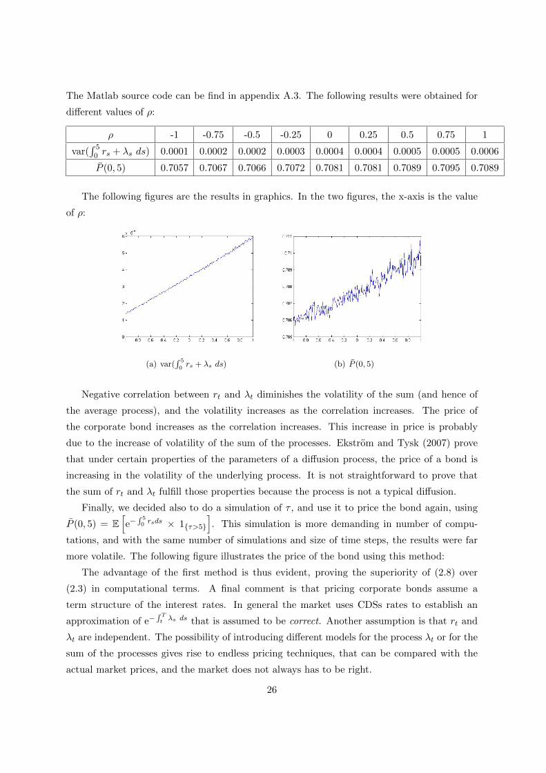
The Matlab source code can be find in appendix A.3. The following results were obtained for

different values of ρ:

ρ -1 -0.75 -0.5 -0.25 0 0.25 0.5 0.75 1

var(∫ 5

0 rs + λs ds) 0.0001 0.0002 0.0002 0.0003 0.0004 0.0004 0.0005 0.0005 0.0006

P (0, 5) 0.7057 0.7067 0.7066 0.7072 0.7081 0.7081 0.7089 0.7095 0.7089

The following figures are the results in graphics. In the two figures, the x-axis is the value

of ρ:

(a) var(∫ 5

0rs + λs ds) (b) P (0, 5)

Negative correlation between rt and λt diminishes the volatility of the sum (and hence of

the average process), and the volatility increases as the correlation increases. The price of

the corporate bond increases as the correlation increases. This increase in price is probably

due to the increase of volatility of the sum of the processes. Ekstrom and Tysk (2007) prove

that under certain properties of the parameters of a diffusion process, the price of a bond is

increasing in the volatility of the underlying process. It is not straightforward to prove that

the sum of rt and λt fulfill those properties because the process is not a typical diffusion.

Finally, we decided also to do a simulation of τ , and use it to price the bond again, using

P (0, 5) = E[e−

∫ 50 rsds × 1{τ>5}

]. This simulation is more demanding in number of compu-

tations, and with the same number of simulations and size of time steps, the results were far

more volatile. The following figure illustrates the price of the bond using this method:

The advantage of the first method is thus evident, proving the superiority of (2.8) over

(2.3) in computational terms. A final comment is that pricing corporate bonds assume a

term structure of the interest rates. In general the market uses CDSs rates to establish an

approximation of e−∫ Tt λs ds that is assumed to be correct. Another assumption is that rt and

λt are independent. The possibility of introducing different models for the process λt or for the

sum of the processes gives rise to endless pricing techniques, that can be compared with the

actual market prices, and the market does not always has to be right.

26

Figure 4.2: P (0, 5) simulating τ

27

Chapter 5

Conclusion

Credit risk is the risk associated to claims that have a positive probability of default.

Credit risk is important because investors are not guaranteed to get the expected return on

their investments, but instead they can lose their invested capital if default occurs.

In this thesis we studied the modeling of credit risk through intensity models. The general

approach of these models is to model the default event τ as the first jump of a Poisson process.

The survival probability of τ takes the form of a discount factor, and the default intensity plays

the same role as an interest rate process. This default intensity can be modeled as a constant,

as a deterministic time-varying function, or as a stochastic process.

We studied a general valuation formula of claims subject to credit risk considering a stochas-

tic default intensity. The formula is general in the sense that it can be applied to any claim

subject to credit risk, and is independent of the structure of the default intensity. In particu-

lar, the formula does not assume independence between the default intensity and the risk-free

process. The case where the contingent claim is a corporate bond was studied with more detail.

The Credit Default Swap (CDS) is an instrument that provides an option to investors to

mitigate credit risk. The pricing of a model independent CDS was studied, as well as the

particular case where the default intensity is independent of the risk-free process. A usual

market practice of “stripping” survival probabilities from CDS quotes was also studied.

Finally, we studied the pricing effects in corporate bonds of inducing different correlations

between the default intensity and the risk-free process. In particular, a negative correlation

between the processes lowers the volatility of the sum of the processes. This lowers the price

of the corporate bond, and the price increases with the correlation. Additionally, and for this

particular claim, it was seen that it is more efficient to discount the cashflow with the sum of

the risk-free process and the credit spread, than to simulate the default event by itself. Further

proposed research include if this superiority is also evident in other contingent claims subject

to default risk.

28

Appendix A

Matlab Source Codes

A.1 CDS pricing

%CDS pricing function

%a=Beginning time of the CDS (usually 0)

%b=Maturity in years of the CDS

%s=Market quote

%L=Loss given default

%gamma=Intensity vector

%PEURC=Default-free zero-coupon bond prices

function z=CDS(a,b,s,L,gamma,PEURC);

j=(b-a)*4;

Gamma_j=zeros(1,j+1);

for i=2:(j+1)

Gamma_j(i)=Gamma_j(i-1)+gamma(i);

end

fir=0;

sec=0;

thir=0;

for i=1:j

fir=fir+gamma(i)*quad(@(u)FIRST(u,Gamma_j,gamma,PEURC,i-1),i-1,i);

sec=sec+exp(-Gamma_j(i))*PEURC(i*90);

thir=thir+gamma(i)*quad(@(u)THIRD(u,Gamma_j,gamma,PEURC,i-1),i-1,i);

29

end

fir=s*fir;

sec=s*sec;

thir=L*thir;

z=fir+sec-thir;

return;

%First argument auxiliary function for the CDS pricing

function y=FIRST(u,Gamma_j,gamma,PEURC,mmin)

days=floor(u*90);

days(days == 0) = 1;

y=exp(-Gamma_j(mmin+1)-gamma(mmin+2).*(u-mmin)).*PEURC(days)’.*(u-mmin);

return;

%Third argument auxiliary function for the CDS pricing

function y=THIRD(u,Gamma_j,gamma,PEURC,mmin)

days=floor(u*90);

days(days == 0) = 1;

y=exp(-Gamma_j(mmin+1)-gamma(mmin+2).*(u-mmin)).*PEURC(days)’;

return;

A.2 Code for stripping out constant intensities

%Function to strip out constant intensities

%L=Loss given default

%ba=Maturity terms

%sa=Market quotes

%gammai=Intensity parameters

function z=calib(PEURC);

L=1-0.15;

ba=[1 3 5 7 10];

%sa=[.01925 .0215 .0225 .0235 .0235];

%sa=[.0725 .0630 .0570 .0570 .0570];

%sa=[.1450 .1200 .0940 .0850 .0850];

sa=[.5050 .2100 .1500 .1250 .1100];

30

gamma1=.05;

gamma2=.05;

gamma3=.05;

gamma4=.05;

gamma5=.05;

gamma1=fzero(@(gamma1)CDS(0,ba(1),sa(1)/4,L,[[gamma1/4*ones(1,5)]

[gamma2/4*ones(1,8)] [gamma3/4*ones(1,8)] [gamma4/4*ones(1,8)]

[gamma5/4*ones(1,12)]],PEURC),gamma1);













z=[gamma1;gamma2;gamma3;gamma4;gamma5];

return;

A.3 Code for pricing a defaultable corporate bond

% Corporate bond pricing simulation with r and lambda

function [Y]=simr;

T=5; %years

j=100; %time steps by year

n=35000; %number of simulations

deltat=1/j;

%r process parameters

31

k=0.3;

theta=0.05;

r0=0.05;

sigma1=0.1;

%lambda process parameters

g=0.3;

gamma=0.02;

lambda0=0.02;

sigma2=0.06;

J=T*j;

zz=0.01;

RES=zeros(3,2/zz+1);

for m=1:(2/zz+1)

rho=(m-1)/(1/zz)-1 %different values of the correlation

if rho==1

C2=[1 1; 0 0];

elseif rho==-1

C2=[1 -1; 0 0];

else

C2=chol([1 rho;rho 1]);

end

R=zeros(n,J+1);

L=zeros(n,J+1);

INT=zeros(n,J);

R(:,1)=r0;

L(:,1)=lambda0;

for i=2:(J+1)

ale=randn(n,2)*C2;

deltar=k*(theta*ones(n,1)-R(:,i-1))*deltat +

sigma1 * sqrt(deltat) * sqrt(R(:,i-1)).*ale(:,1);

R(:,i)=max(0.0001,R(:,i-1)+deltar);

32

deltal=g*(gamma*ones(n,1)-L(:,i-1))*deltat +

sigma2 * sqrt(deltat) * sqrt(L(:,i-1)).*ale(:,2);

L(:,i)=max(0.0001,L(:,i-1)+deltal);

if i==2

INT(:,i-1)=(R(:,i-1)+L(:,i-1))*deltat;

else

INT(:,i-1)=(R(:,i-1)+L(:,i-1))*deltat+INT(:,i-2);

end

end

RES(1,m)=rho;

RES(2,m)=var(INT(:,J)/T);

RES(3,m)=mean(exp(-INT(:,J)));

end

Y=RES;

return;

33

Bibliography

[1] Bielecki, T., and Rutkowski, M. Credit Risk: Modeling, Valuation and Hedging,

first ed. Springer, 2002.

[2] Bjork, T. Arbitrage Theory in Continuous Time, second ed. Oxford University Press,

2004.

[3] Black, F., and Scholes, M. The pricing of options and corporate liabilities. Journal of

Political Economy 81, 3 (1973), 637–654.

[4] Brigo, D., and Mercurio, F. Interest Rate Models - Theory and Practice, second ed.

Springer, 2006.

[5] Cox, J., Ingersoll, J., and Ross, S. A theory of the term structure of interest rates.

Econometrica 53, 2 (1985), 385–407.

[6] Duffie, D., and Singleton, K. Modeling term structures of defaultable bonds. The

Review of Financial Studies 12, 4 (1999), 687–720.

[7] Ekstrom, E., and Tysk, J. Convexity theory for the term structure equation. Finance

Stochastic 12 (2008), 117–147.

[8] Merton, R. Theory of rational option pricing. The Bell Journal of Economics and

Management Science 4, 1 (1973), 141–183.

[9] Morris, C., Neal, R., and Rolph, D. Credit spreads and interest rates: A cointegration

approach. Federal Reserve Bank of Kansas City (1998).

34

modeling credit risk through intensity...

Documents