A Spline Algorithm for Modeling Cutting Errors on

Turning Centers

David E. Gilsinn#

Herbert T. Bandy

Automated Production Technology Division National Institute of Standards and Technology

100 Bureau Drive-Stop 8220 Gaithersburg, MD 20899-8220

Alice V. Ling

AFRL/DEBS 3550 Aberdeen Ave SE

Kirtland AFB, NM 87117-5776

#Corresponding Author

NISTIR 6517 May 2000

Abstract

Turned parts on turning centers are made up of features with profiles defined by arcs and lines. An error model for turned parts must take into account not only individual feature errors but also how errors carry over from one feature to another. In the case where there is a requirement of tangency between two features, such as a line tangent to an arc or two tangent arcs, any error model on one of the features must also satisfy a condition of tangency at a boundary point between the two features. Splines, or piecewise polynomials with differentiability conditions at intermediate or knot points, adequately model errors on features and provide the necessary degrees of freedom to match constraint conditions at boundary points. The problem of modeling errors on features becomes one of least squares fitting of splines to the measured feature errors subject to certain linear constraints at the boundaries. The solution of this problem can be formulated uniquely using the generalized or pseudo inverse of a matrix. This is defined and the algorithm for modeling errors on turned parts is formulated in terms of splines with specified boundary constraints. Key Words: error modeling; generalized inverse; least squares; machine tool; pseudo inverse; spline

1.0 Introduction

Errors in a machined part are due to several sources. There are errors inherent in the

machine itself due, for example, to misalignment of slide ways and other geometric

errors. There are errors due to thermal deformations of the machine while operating.

There are also errors caused by inaccurately specified tool dimensions, tool wear, tool

and/or part deflection, and so on. We will call these types of errors the “process related

errors”. It is the modeling of these process related errors for a turning center that will

concern us in this report.

The object of developing process error models is to apply them in error compensation

strategies (Donmez et al. 1991) (Bandy 1991). Process errors can be measured during

machining (Fan and Chow 1991) or by process intermittent gauging. Process-

intermittent gauging has an advantage in that a simple measurement device, such as a

touch-trigger probe, can be inserted into the tool changer. This form of probe is less

intrusive than apparatus required for measurement during machining. Process-

intermittent gauging of process-related part errors usually takes place between semi-

finish and finish machining processes. This permits on-line modeling of process-related

errors, the results of which are then used to anticipate and compensate these errors in the

finish process. For a discussion of process-intermittent probing and real-time error

compensation (Yee 1990) (Yee and Gavin 1990).

One form of error compensation strategy requires interpreting a part as consisting of

separate features. Such a decomposition of a part is useful for establishing

2

correspondence between design information and manufacturing operations (Gupta et al.

1995). Part features can be defined very generally. For a turning center, however, in

which part geometry is defined in two dimensions, the features of concern are the arcs

and lines that comprise the CAD profile of the part. CAD-based methods facilitate the

creation of pre-process data such as feature geometry, nominal coordinates of gauging

points, and surface normal vectors.

Any error model for turned parts must take into account not only errors on individual

features but also how the errors carry over from one feature to another. This just reflects

the physical fact that as a tool cuts a feature of a part it transitions in a smooth manner to

cutting the next feature. This implies that there should not be any unintentional changes

in slopes between features. Therefore, a feature error model must take into account slope

constraints at the ends of the features.

Another aspect of modeling machine tool errors is the need to create model function

forms that can be computed rapidly when the models are implemented in error

compensation strategies. This often means that functional forms need to be low order

polynomials. However, low order polynomials may or may not model all the errors on a

machined feature. If the geometry of a feature is broken into smaller parts, the errors on

those smaller parts can often be modeled by low order polynomials. If the low order

polynomials are chosen in such a way that the slopes are made equal at the feature part

transition points, the combined piecewise polynomial is called a spline (DeBoor 1978).

3

The error-modeling algorithm described in this report combines the use of splines, to

model the errors within a feature, with boundary slope constraints at the ends of the

features. The general modeling technique involves a least squares fitting of a spline to

process-intermittent, measured, machine-error data but with an extra requirement that

slopes at the end of features be equal. These are usually linear constraints so the

algorithm can be classified as a least squares fitting of a linear model with linear end

constraints.

2.0 Modeling Errors on Features with Linear Profiles

When linear features join each other the modeling does not necessarily require splines

but splines could be used. Regardless of whether splines are used, at least two cases of

errors usually occur. First, if an analysis of the part errors indicates the existence of

feature size errors only, a constant offset for either axis is sufficient to compensate the

errors. In this case, the compensation software inserts the appropriate values in the tool

offset update command in the numerical control (NC) program segment for the finish cut

and all coordinates in the NC program are left at their nominal values. As an alternative

means of compensating such errors, the compensation software also writes the axis

offsets to a file, which is used for real-time compensation. Second, if errors are

essentially linear but the slopes are different from those of the nominal features, the

compensation software can adjust the finish cuts for each feature. Adjustments for

features with nominally linear profiles are usually calculated by fitting linear functions

through the error vectors computed at the gauge points for each cut of the part. The

4

intersections of the linear equation for a cut with similar linear error equations for the

neighboring cut on each side give the errors at the endpoints of the cut. These endpoint

errors are used to adjust the points that are then entered into NC program for the finish

cut and are written to a file that is used to provide data to generate real-time cut

adjustments. Elaboration of these procedures may be found in (Bandy and Gilsinn 1996)

(Bandy and Gilsinn 1995a) (Bandy and Gilsinn 1995b).

3.0 Modeling Errors on Features with Curved Profiles

If a part contains a feature whose nominal profile is not linear, the adjustments are more

complex. For example, when an arc smoothly meets a line or another arc, not only do the

compensation curves intersect but the two curves must usually be tangent to each other.

The treatment of a circular arc profile is explained in this section. The principles,

however, can be extended to non-circular curves.

Some earlier work in compensating errors on a hemispherical nose of a turned part

showed that error compensation on arcs was feasible (Yee et al. 1992). No attempt,

however, was made in this previous work to maintain tangencies at feature boundaries.

Although the previous work showed that process-intermittent errors in curved features

could be compensated, the application was limited to a turned hemisphere generated by a

nominal arc cut, because a circle could be fitted to the probed data. However, turning

centers can generate other types of curved cuts, which are better fitted by spline

modeling. Furthermore, the previous work did not consider what would happen at the

5

interface between two features such as a linear feature tangent to a curved feature. If two

curves are fit separately to probed values on each feature, then the resulting curves might

have a discontinuity at the nominal point of tangency. In the finish cut, this could lead to

a significant step in the part. Therefore, another data fitting procedure had to be

investigated to compensate errors on general, turned, curved features that might have

various interface angles to neighboring features. That is, a least squares technique with

prescribed boundary conditions had to be developed. This problem cannot be treated as a

standard least squares problem since the boundary conditions restrict the selection of the

fitting parameters.

Polynomials are useful as approximation functions to unknown and possibly very

complex nonlinear relationships. However, the literature on least squares regression

models (Smith 1979) (Wold 1974) warns that it is important to keep the order of the

polynomial models as low as possible. In an extreme case it is possible to pass a

polynomial of order n-1 through n points so that the polynomial of sufficiently high

degree can always be found that provides a "good" fit to the data. The behavior of the

polynomial between the data points may be highly oscillatory, though, and not provide

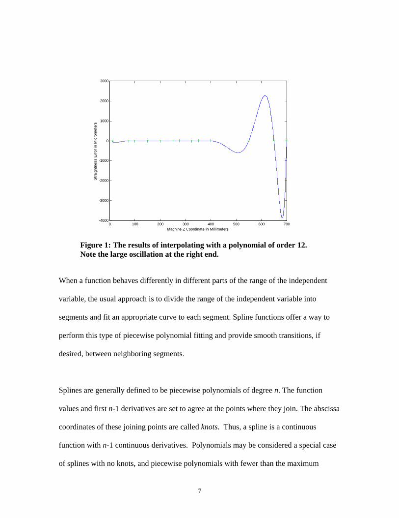
good data interpolation. Figure 1 is a good example of the oscillatory behavior of a high

order interpolating polynomial. The probe data in the figure represents micrometer errors

measured on the Z-axis of travel on a turning center. Notice that the interpolating

polynomial goes through each of the data points, but only produces a good fit between

the data points within the mid-range of the data. The interpolating polynomial, however,

performs large excursions near the ends of the data set. This is a typical behavior of a

high order interpolating polynomial.

6

When

variab

segme

perfor

desire

Spline

value

coord

functi

of spl

0 100 200 300 400 500 600 700-4000

-3000

-2000

-1000

0

1000

2000

3000

Stra

ight

ness

Erro

r in

Mic

rom

eter

s

Machine Z Coordinate in Millimeters

Figure 1: The results of interpolating with a polynomial of order 12. Note the large oscillation at the right end.

a function behaves differently in different parts of the range of the independent

le, the usual approach is to divide the range of the independent variable into

nts and fit an appropriate curve to each segment. Spline functions offer a way to

m this type of piecewise polynomial fitting and provide smooth transitions, if

d, between neighboring segments.

s are generally defined to be piecewise polynomials of degree n. The function

s and first n-1 derivatives are set to agree at the points where they join. The abscissa

inates of these joining points are called knots. Thus, a spline is a continuous

on with n-1 continuous derivatives. Polynomials may be considered a special case

ines with no knots, and piecewise polynomials with fewer than the maximum

7

number of continuity restrictions may also be considered splines. The number and

degrees of the polynomial pieces and the number and position of the knots may vary in

different situations.

Figure 2 shows the results of interpolating the same probe data as in Figure 1 but using a

clamped spline (note that the scale of the ordinate axis is different from Figure 1). A

clamped spline means one with prescribed derivative conditions specified at the end

points of the data. This figure shows vividly the benefits of interpolating with spline

functions. The ability to interpolate with piecewise polynomial allows a tighter control on

the interpolation errors.

4.0 Constructing Interpolating Splines with End Constraints

0 100 200 300 400 500 600 700-3

-2

-1

0

1

2

3

4

5

6

7

Machine Z Coordinate in Millimeters

Stra

ight

ness

Erro

r in

Mic

rom

eter

s

Figure 2: Interpolating the same data from Figure 1 using a clamped cubic spline. Note the close modeling of the data.

It is possible to construct a basis, or sequence of functions, such that every spline of

interest can be written in one and only one way as a linear combination of these functions

(Montgomery and Peck 1992). General cubic splines ( n = 3) will be used since they have

8

been shown to be adequate for most practical problems. They can be written in terms of

basis functions as follows:

Let an ordered sequence of k knots be given. These can be nominal probe points, but do

not necessarily have to be

A cubic spline with these k kno

The are cons3,,1, += kjc j

y

)

bt<...<t<ta k21 ≤≤ (1

ts can be written as

tants and

) t - (x c + x c = (x) 3+j3 +j

k

1 =j

jj

3

0 =j ∑∑ (2)

⎪⎩

⎪⎨⎧

≤ t x 0 t> x ) t - (x

= ) t - x (j

j3

j3+j (3)

9

This cubic spline representation has continuous first and second derivatives. See (Smith

1979) (Wold 1974) for good general discussions of the use of splines in statistical data

analysis.

Assume that there are s sampled points in the plane given by the pairs

and suppose that the x-values are ordered by ),(,),,( 11 ss yxyx

where a and b are bounds for the sequence of x-values. Since the sampled points might

show undesired oscillations or Anoise@, some form of smoothing will be obtained by not

selecting knots at each point. In fact, guidelines in the literature (Smith 1979) (Wold

1974) suggest 4 to 5 points between knots. Since this will not always be possible one can

select this value as a variable, say r, and set a knot at every r-th point. This would mean

that one first selects an integer k so that skr ≤ . This selection of knots partitions the

sampled points into the sets

b, x < ... < x < x a s21 ≤≤ (4)

.x <...< x < )t(= x <...x < )t(= x <...< x < ) t= ( x <

...<x<x

s1+rk

nr k1+r 22r 21+r1r

21

(5)

10

The standard least squares problem of fitting a spline of the form (2) through the sample

points can be formulated in matrix terms. To start, with define the residual at the q-th

sample point q = 1, 2, …,s, as

⎪⎪⎩

⎪⎪⎨

⎧

≥

<

∑∑

∑

r q ) t - x( c - x c - y

r q x c - y = R

3jq3 +j

t

1 =j

jqj

3

0 =j q

jqj

3

0 =j q

q (6)

where, for a given q-th point, t is the smallest integer so that strq ≤≤ . To begin

formulating the matrix version of the least squares problem define the vectors

TT

where the superscript T in

formulated as

)y ,...,y ( =y ,) c ,...,c ( = c s13 + k0

dicates a transposed vector. The least squares sum is usually

2s

.) R ( = ) c ( LS q1 = q

∑ (8)

11

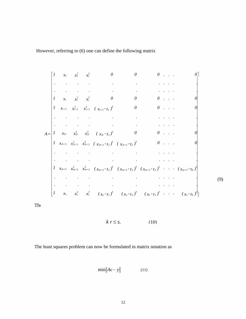
However, referring to (6) one can define the following matrix

The matrix A is s rows by k + 4 columns where

⎥⎥⎥⎥⎥⎥⎥⎥⎥⎥⎥⎥⎥⎥⎥⎥⎥⎥⎥⎥⎥⎥⎥⎥⎥⎥⎥⎥

⎦

⎤

⎢⎢⎢⎢⎢⎢⎢⎢⎢⎢⎢⎢⎢⎢⎢⎢⎢⎢⎢⎢⎢⎢⎢⎢⎢⎢⎢⎢

⎣

⎡

)t - x(...)t - x()t - x()t - x(xxx1

...........

...........

)t - x(...)t - x()t - x()t - x(xxx1

...........

...........

0...0)t- x ()t - x (xxx1

0...00)t - x (xxx1

...........

...........

0...00) t - x (xxx1

0...000xxx1

...........

...........

0...000xxx1

= A

3ks

33s

32s

31s

3s

2ss

3k1+nr

331+nr

321+nr

311+nr

31+nr

21+nr1+nr

321+2r

311+2r

31+2r

21+2r1+2r

312r

32r

22r2r

311+r

31+r

21+r1+r

3r

2rr

31

211

(9)

The least squares problem can now be formulated in matrix notation as

s.rk ≤ (10)

yAc−min (11)

12

where the minimum is taken over all vectors c and the norm is the standard Euclidean

norm.

The splines in this application are not unrestricted at their ends, however, and this changes

the least squares problem in this case. In order to make the curved features match with

neighboring features, restrictions must be placed on how the splines behave at the

endpoints a and b of the interval. In particular, we will require that the splines go through

specific points with specific slopes. Therefore, we will require the following conditions be

satisfied:

where the right hand sides are prescribed by the matching requirements. These conditions

y = )t - (b c 3 + b cj

y = a cj

y = )t - (b c + b c

y = a c

(1)1+s

2j3j+

k

1=j

-1jj

3

1=j

(1)0

-1jj

3

1=j

1+s3

j3j+

k

1=j

jj

3

0=j

0j

j

3

0=j

∑∑

∑

∑∑

∑

(13)

y = (b)dxdy

y = (a)dxdy

y = y(b)y = y(a)

(1)1+s

(1)0

1+s

0

(12)

13

can also be formulated as matrix equations. To do this, first write each of the conditions

as

then define

⎥⎥⎥⎥⎥⎥

⎦

⎤

⎢⎢⎢⎢⎢⎢

⎣

⎡

)t - 3(b...)t - 3(bb32b10

0...0a32a10

)t - (b...)t - (bbbb1

0...0aaa1

= B

2k

212

2

3k

3132

32

(14)

and let

.)y ,y ,y ,y ( = f T(1)1+s

(1)01+s0 (15)

The constraint equation becomes The constrained least squares proble

solution of this problem requires de

If A is an n x n nonsingular matrix t

given uniquely by c = A-1y. But in t

columns and m and n are not the sam

matrix Z so that c = Zy where c is th

squares problem (11). In fact the an

f. = c B (16)

m is then the combined relations (11) and (16). The

fining a generalized notion of an inverse of a matrix.

hen the solution of the matrix problem Ac = y is

he least squares problem where A has m rows and n

e value, the question arises whether there is an n x m

e unique minimum length solution of the least

swer is yes, and the matrix Z is uniquely determined

14

by A. It is called the generalized or pseudo inverse of A, and is denoted by A+ (Lawson

and Hanson 1974).

It is not difficult to find the generalized inverse of a matrix A if A is properly

decomposed. For this application one can introduce the decomposition of A called the

singular value decomposition (Lawson and Hanson 1074). Any m x n matrix A, whose

number of rows m is greater than or equal to the number of columns n, can be written as

the product of an m x n column orthogonal matrix U, an n x n diagonal matrix D, and the

transpose of an n x n orthogonal matrix V. Symbolically

V D U = A T (17) where and I is the n x n identity matrix and D

d = D where dii could be zero for several i=s.

A+ where

diag = D+ and

=+dii

I = U U T

I=VV T (18)

is the diagonal matrix

]d ..., ,d ,d[ iag nn2211 (19)

The generalized inverse of A can be written as

U D V = T+ (20)

]d ..., ,d ,d [ +nn

+22

+11 (21)

15⎪⎩

⎪⎨⎧

≤

>

told

toldd

ii

iiii

0

1 (22)

and tol is a tolerance that is often set in such a way that it is related to the reciprocal of

the maximum allowed condition number (i.e. ratio of the largest eigenvalue to the

smallest) for the matrix D.

One can now formulate the result that gives the solution to the constrained least squares

problem (11), (16). The principal reference for this result is (Lawson and Hanson 1974).

Given an m x n matrix B of rank k, an m-vector y, an r x n matrix A, and an r-vector y the

linear least squares problem with equality constraints becomes one of finding an n-vector

c that minimizes

fAc− (23)

and satisfies the linear equalities

f. = c B (24)

This is just a general restatement of the problem described by (11) and (16) above.

16

Assuming that (24) is consistent, there is a unique solution that minimizes (23) subject to

(24) (Wold 1974). It is given by

) f AB -y ( ) Z(A + f B = c +++ (25)

where

B B - I = Z +n (26)

and In is the n x n identity matrix. For many usual cases one would have n > r = k. The

generalized inverses are computed by the singular value decomposition technique.

In order to use the spline representation of the surface errors on a part it is easier to

evaluate the spline in its individual cubic components between knots. To do this requires

compacting the representation of the spline polynomial as the underlying variable passes

each knot. The algorithm is straightforward and begins by assuming that there are k

knots. First add two knots for the end points to make k+2 knots. Thus,

b. = t < t <...< t < t= a (27)

1+kk10

17

For k internal knots there will be k+4 spline coefficients. But when these are combine to

form groups of four coefficients for each interval there will be 4k+4 coefficients. These

will be defined as follows: For

t x t = a 10 ≤≤ (28)

the polynomial is given by

x c + x c + x c+ c = y(x) 3*

42*

3*2

*1 (29)

where

That is, the first four coefficients of the new array, identified by the superscript asterisk,

are the same as the spline coefficients. The other groups of four coefficients are

computed as follows. For j = 1, 2, ..., k one has for

c = cc = cc = cc = c

4*4

3*3

2*2

1*1

(30)

t x t 1+jj ≤≤ (31)

the polynomial

18

x c + x c + x c+ c = y(x) 3*4+4j

2*3+4j

*2+4j

*1+4j (32)

where

5.0 Model Application

The part used to demonst

portion on the largest dia

The software, in which th

Intermittent Error Compe

compensate machining er

part in Figure 3 was chos

- = 3**

c + c = ct c 3 - c = ct c 3 + c = c

tccc

4+j*

4+1)-4(j*

4+4j

j4+j*

3+1)-4(j*

3+4j

2j4+j

*2+1)-4(j

*2+4j

j4+j1+1)-4(j1+4j

(33)

rate the use of the algorithm is shown in Figure 3. It has a step

meter area, a long taper, a cylindrical section and a hemisphere.

e algorithm described in this report is embedded, called Process

nsation Software (PIECS) (Bandy and Gilsinn 1996), is used to

rors on all of these surfaces. The tool tip selected to turn the

en from a batch that were known to be worn but the exact nature

19

of the wear was unknown at the time of selection. The authors thought that this would be

a good test of the algorithm, since the errors generated at the semi-finish cut would be

unknown beforehand to the operator. The resulting semi-finish part showed errors that

indicated the worn spot lay at approximately a 450 angle on the tool tip. This is indicated

by the errors plotted in Figure 4. The errors are shown as scaled bars that are called

“whiskers”. These errors are reflected in the probed errors reported in Table 1, which are

errors normal to the surfaces averaged for four parts. The values are in micrometers.

After applying the spline algorithm to model the errors on the front dome and small linear

feature to its left on the semi-finish cut, the errors were considerably reduced on the

finish cut as shown in Table 1, and the “whiskers” plot in Figure 5. Figure 6 shows the

spline model of the errors on the leading two features of the part with a zero slope

specified at the boundary point with the linear feature and a slightly greater than zero

slope specified at the part zero point near the right hand corner of Figure 6.

6.0 Conclusions

Compensation of process related errors based on process-intermittent measurements and

modeling has shown in the past that the procedure can correct errors on parts with linear

features (Bandy and Gilsinn 1996) (Bandy and Gilsinn 1995a) (Bandy and Gilsinn

1995b). This procedure has been extended to correcting errors on parts with arc features.

In order to maintain path and slope continuity between tangent features, it was necessary

to use splines with boundary constraints.

20

The splines with constraints have been demonstrated to adequately model machining

errors probed on semi-finished parts. These models have successfully been used to reduce

the part errors on the finish part to a small fraction of the original errors on the semi-

finished part. In fact, the models allow the same tool that caused the errors to be used to

correct them. Table 1 clearly shows the magnitude of reduction obtained.

The algorithm presented in this report allows the splines to be represented in the compact

form of equation (29). This ensures that the resulting polynomials are of low order so that

they can be used in error compensation during machining processes. That is, the error

model evaluation time is not a significant factor to the error compensation process.

21

Figure 3: Part with Hemispherical Dome used to Test Algorithm

22

Mean Turning Center Errors for Four Parts

Point Number

Nominal XGauging

Coordinate (mm)

Nominal ZGauging

Coordinate (mm)

Semi-finish Part Error (µm)

Finish Part Error (µm)

1 63.87211 -149.1631 90.297 -0.5715 2 60.46455 -143.0105 92.71 -0.889 3 57.05696 -136.858 92.964 -1.651 4 53.6494 -130.7054 94.1705 -0.762 5 50.24184 -124.5529 92.5195 -3.175 6 44.704 -106.934 12.446 -0.254 7 44.704 -92.0115 11.176 -0.508 8 44.704 -77.089 10.9855 -2.54 9 44.704 -62.1665 11.684 -3.048 10 44.704 -47.244 12.446 -2.286 11 43.434 -44.704 0 0 12 37.084 -38.354 6.731 -3.302 13 36.99706 -34.54598 21.717 7.8105 14 36.70041 -31.76392 31.623 3.2385 15 36.19487 -29.01213 44.577 -1.8415 16 35.48329 -26.30632 52.705 -4.7625 17 34.56976 -23.66183 62.8015 -2.54 18 33.45945 -21.09373 69.977 1.016 19 32.15869 -18.61668 76.2 1.778 20 30.67487 -16.24472 78.359 -0.762 21 29.01645 -13.99139 77.2795 -3.429 22 27.19286 -11.8695 76.7715 -1.397 23 25.2145 -9.891141 70.9295 -3.429 24 23.09261 -8.067548 63.5 -3.2385 25 20.83928 -6.409131 58.8645 -1.651 26 18.46732 -4.925314 51.435 -1.524 27 15.99027 -3.624555 45.2755 -3.1115 28 13.42217 -2.514244 36.83 -6.0325 29 10.77768 -1.600708 32.9565 -5.842 30 8.071866 -0.889127 27.432 1.651 31 5.320081 -0.383591 8.0645 -0.8255 32 2.538019 -0.086944 -18.733 -8.636

Table 1: Semi-finish and Finish Errors for Turned Part

23

Figure 4: A “whiskers” plot of the Errors on the Semi-Finish Part

Figure 5: “Whiskers” Plot of the Reduced Errors on the FinishPart

24

X Part Coordinates in mm

Z Part Coordinates in mm

-45 -40 -35 -30 -25 -20 -15 -10 -5 0 50

5

10

15

20

25

30

35

40

45

50

Spline Model Of Errors

Linear Profile

Dome Profile

Scaled Error Bars

X Part Coordinates in mm

Z Part Coordinates in mm

Figure 6: Scaled Semi-Finish Errors in Micrometers on the Leading Dome Profile and Linear Feature to the Left of the Dome Profile. See Points 12 through 32 in Table 1.

25

7.0 References

Bandy, H.T. (1991) Process-Intermittent Error Compensation, NISTIR 4536, Progress

Report of the Quality in Automation Project for FY90, M.A. Donmez (Ed.)., National

Institute of Standards and Technology, Gaithersburg, MD: 25-39;.

Bandy, H. T., Gilsinn, D. E. (1995a) Data Management for Error Compensation and

Process Control, SPIE Proceedings on Modeling, Simulation, and Control Technologies

for Manufacturing, Vol. 2596, 114-123.

Bandy, H. T.; Gilsinn, D. E. (1995b) Compensation of Errors Detected by Process-

Intermittent Gauging. Proceedings of the American Society for Precision Engineering

1995 Annual Meeting ; 12; October 15-20; Austin, TX.

Bandy, H.T., Gilsinn, D. E. (1996) PIECS-A Software Program for Machine Tool

Process-Intermittent Error Compensation, NISTIR 5797, National Institute of Standards

and Technology.

De Boor, C. (1978) A Practical Guide to Splines. Springer-Verlag, New York.

Donmez, M.A., Yee, K.W., Neumann, D.H., Greenspan, L. (1991) Implementing Real-

Time Control for Turning Center, NISTIR 4536, Progress Report of the Quality in

26

Automation Project for FY90, M.A. Donmez (Ed.)., National Institute of Standards and

Technology, Gaithersburg, MD, 25-39.

Fan, K.C., Chow, Y.H. (1991) In-Process Dimensional Control of the Workpiece during

Turning, Precision Engineering, Vol. 13, No 1, 27-32.

Gupta, S.K., Regli, W.C., Nau, D. S. (1995) Manufacturing Feature Instances: Which

Ones to Recognize?, NISTIR 5655, National Institute of Standards and Technology,

Gaithersburg, MD.

Lawson, C. L., Hanson, R. J. (1974) Solving Least Squares Problems Prentice- Hall, Inc.,

Englewood Cliffs.

Montgomery, D., C. Peck, E. A. (1992) Introduction to Linear Regression Analysis ,John

Wiley & Sons, Inc., New York.

Smith, P. (1979) Splines as a Useful and Convenient Statistical Tool. The American

Statistician, 33(2).

Wold, S. (1974) Splines Functions in Data Analysis, Technometrics, 16(1).

27

Yee, K. W. (1990) Real-Time Error Corrector and Process-Intermittent Probing, NISTIR

4322, Progress Report of the Quality in Automation Project for FY89, T. V. Vorburger,

B. Scace (Ed.)., National Institute of Standards and Technology, Gaithersburg, MD, 9-31.

Yee, K. W., Gavin R. J. (1990) Implementing Fast Part Probing and Error Compensation

on Machine Tools, NISTIR 4447, National Institute of Standards and Technology,

Gaithersburg, MD.

Yee, K. W.; Bandy, H. T.; Boudreaux, J.; Wilkin, N. D. (1992) Automated Compensation

of Part Errors Determined by In-Process Gauging, NISTIR 4854, National Institute of

Standards and Technology, Gaithersburg, MD.

28