modeling dispersion under unsteady groundwater flow conditions

Modeling dispersion under unsteady

groundwater flow conditions

Sophie Lebreton

supervised by Amro Elfeki

and Gerard Uffink

• confined aquifer

• upstream water level constant

• downstream water level variable

• constant thickness

• constant hydraulic conductivity K

over the depth

• constant specific storage SS over

the depth

• aquifer modelled in a 2D horizontal

plane

The goal of the study :

investigate the impact of transient flow conditions on solute

transport in porous media

Case study

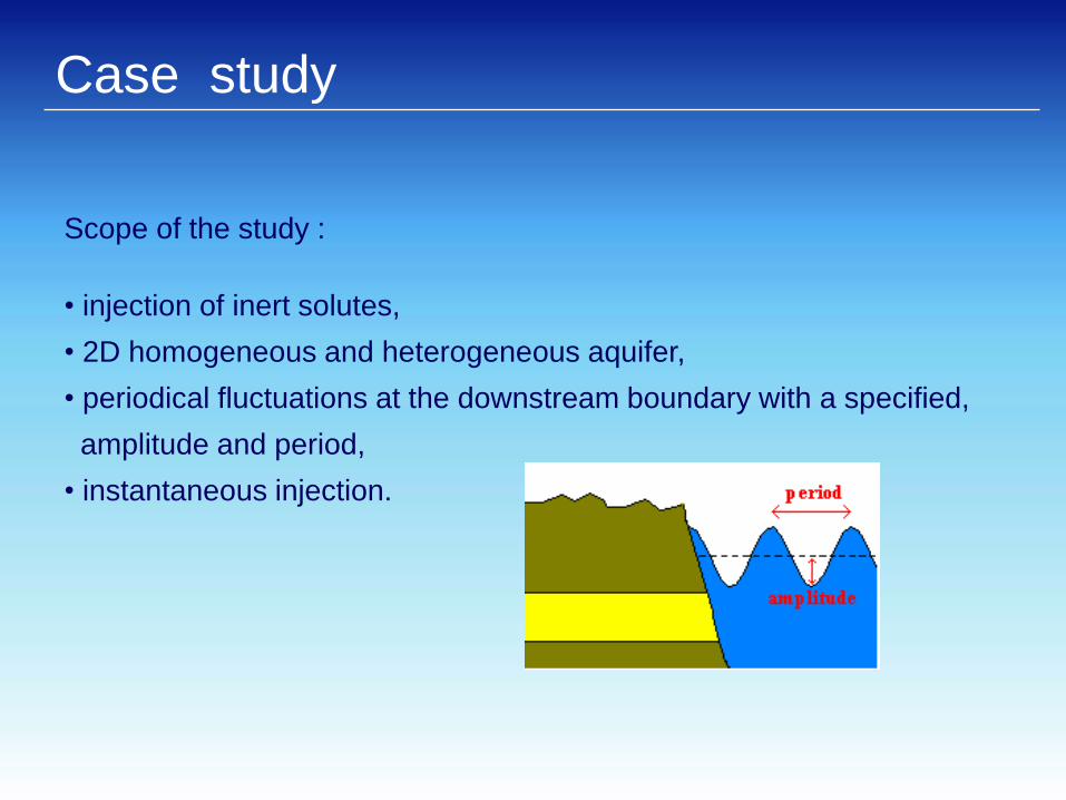
Scope of the study :

• injection of inert solutes,

• 2D homogeneous and heterogeneous aquifer,

• periodical fluctuations at the downstream boundary with a specified,

amplitude and period,

• instantaneous injection.

Case study

Flow model :

• Hydraulic head

• Velocity field

Transport model :

• Concentrations

• Contaminant plume characteristics

2 numerical models

Outlines

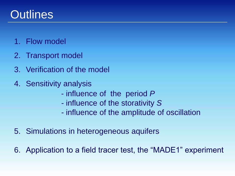
1. Flow model

2. Transport model

3. Verification of the model

4. Sensitivity analysis

- influence of the period P

- influence of the storativity S

- influence of the amplitude of oscillation

5. Simulations in heterogeneous aquifers

6. Application to a field tracer test, the “MADE1” experiment

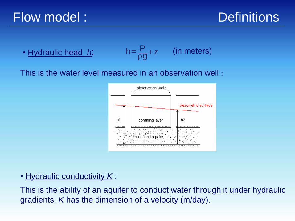
• Hydraulic head h: zPh= g

(in meters)

This is the water level measured in an observation well :

Flow model : Definitions

• Hydraulic conductivity K :

This is the ability of an aquifer to conduct water through it under hydraulic

gradients. K has the dimension of a velocity (m/day).

Governing equation of the flow:

, , , , , ,, ,xx yy

h x y t h x y t h x y tS x y x yT Tt x x y y

Principle of the finite difference method :

• discretization in space

• discretization in time

Flow model : Finite difference method

where h hydraulic conductivity

S the storativity or storage coefficient

T=Kb the transmissivity

0

( , , )0 , (no-flow condition)

(0, , )

( , , ) ( )

h x y tfor x y

nh y t h

h d y t h t

Finite difference formulation of the flow equation :

Implicit scheme :

1 1 1 1 1

, ,1, , 1 1, , 1ij ij ij ij ij ijk k k k k k

i j i ji j i j i j i jF h A h B h C h D h E h

Solution by an iterative scheme : the conjugate gradient

method h(x,y,t)


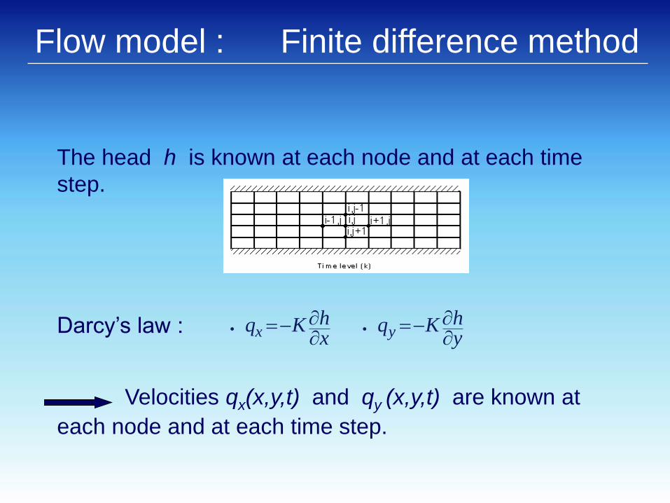
The head h is known at each node and at each time

step.

Darcy’s law :

Velocities qx(x,y,t) and qy (x,y,t) are known at

each node and at each time step.

x yh hq K q Kx y


• Groundwater head :

• Darcy’s velocities :

0 50 100 150 200 250 300

-40

-20

0

Velocity field at a time t

Flow model : outputs

2 transport mechanisms :

Advection : this is the solute flux due to the flow of groundwater

Dispersion : this is due to the velocity variations

Transport model

Gaussian distribution of the concentration

x y xx xy yx yyC C C C C C CV V D D D Dt x y x x y y x y

This equation is not solved directly the random walk

method is used

Principle of the random walk method: pollutant transport is

modeled by using particles that are moved one by one to

simulate advection and dispersion mechanisms.

Transport model : random walk

Governing equation of solute transport :

where C is the concentration

Vx and Vy are pore velocities

Dxx , Dyy , Dxy , Dyx are dispersion coefficients

i j*mij L ij L T

VVD = α V +D δ + α -α

V

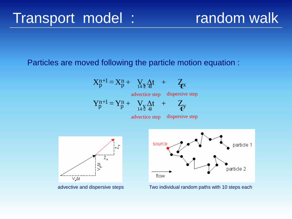
Particles are moved following the particle motion equation :

{

{

dispersive stepadvectice step

dispersive stepadvectice step

n+1 nx xp p

n+1 ny yp p

+ +

+ +

X = X V Δt

Y = Y V Δt

Z

Z

14 2 43

14 2 43

Transport model : random walk

advective and dispersive steps Two individual random paths with 10 steps each

Transport model : algorithm

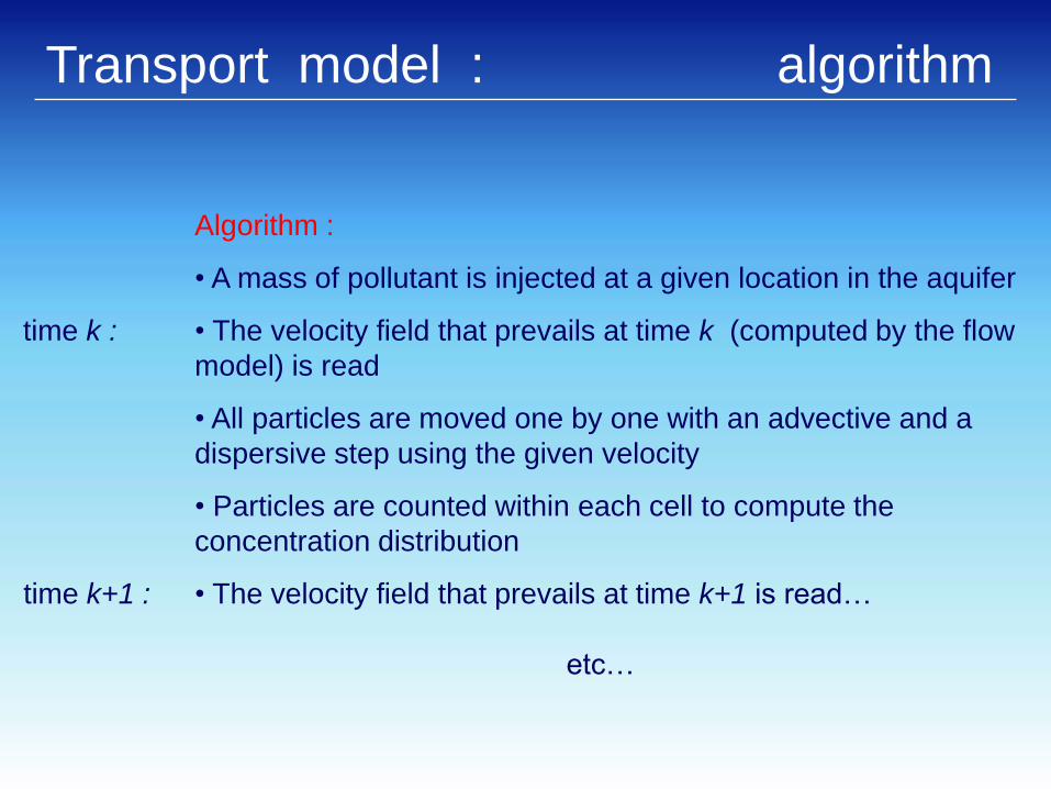
Algorithm :

• A mass of pollutant is injected at a given location in the aquifer

• The velocity field that prevails at time k (computed by the flow

model) is read

• All particles are moved one by one with an advective and a

dispersive step using the given velocity

• Particles are counted within each cell to compute the

concentration distribution

• The velocity field that prevails at time k+1 is read…

etc…

time k :

time k+1 :

Transport model : example

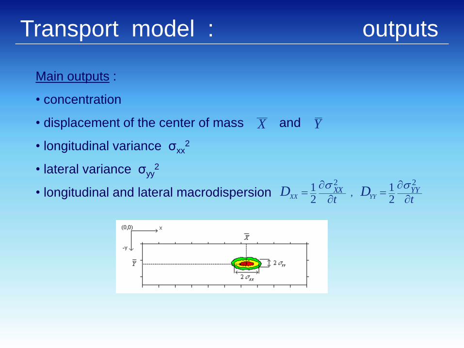
Main outputs :

• concentration

• displacement of the center of mass and

• longitudinal variance σxx2

• lateral variance σyy2

• longitudinal and lateral macrodispersion2 2

,1 12 2XX YY

XX YY

t tD D

Transport model : outputs

X Y

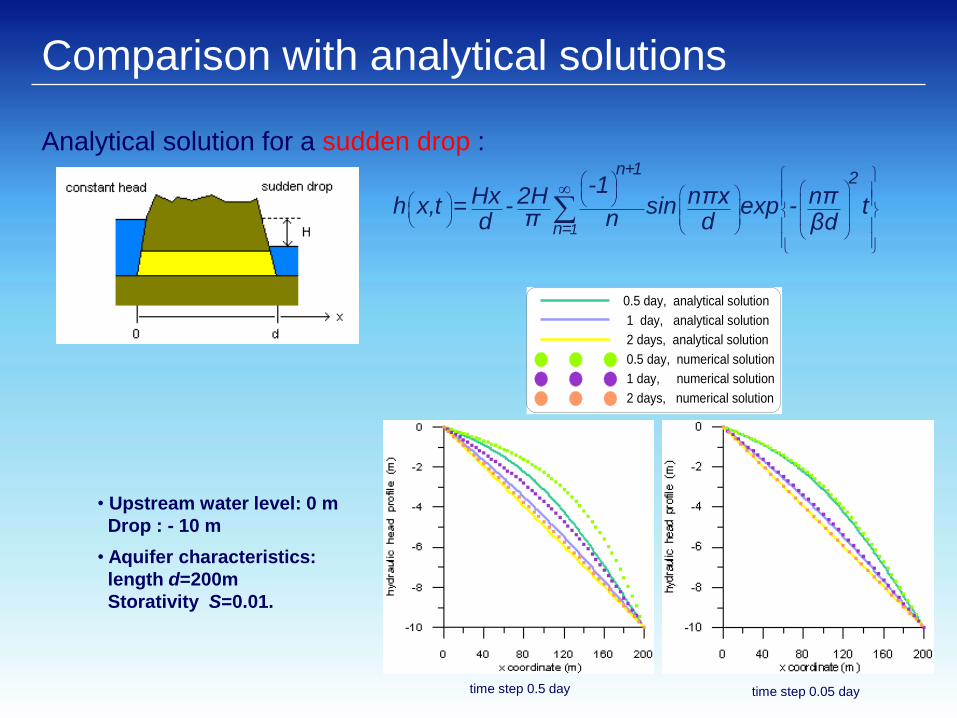
Analytical solution for a sudden drop :

1

n+12

n=

-1Hx 2H nπx nπh x,t = - sin exp - tπ nd d βd

0.5 day, analytical solution

1 day, analytical solution

2 days, analytical solution

0.5 day, numerical solution

1 day, numerical solution

2 days, numerical solution

• Upstream water level: 0 m

Drop : - 10 m

• Aquifer characteristics:

length d=200m

Storativity S=0.01.

time step 0.05 daytime step 0.5 day

Comparison with analytical solutions

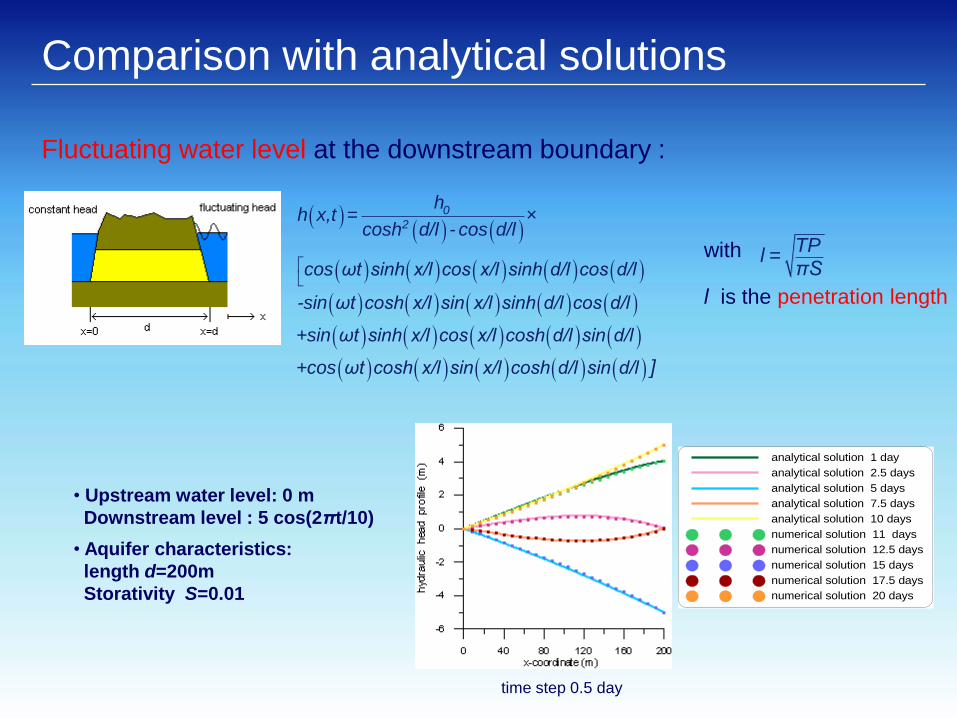
Fluctuating water level at the downstream boundary :

time step 0.5 day

0

2

hh x,t = ×

cosh d/l - cos d/l

cos ωt sinh x/l cos x/l sinh d/l cos d/l

-sin ωt cosh x/l sin x/l sinh d/l cos d/l

+sin ωt sinh x/l cos x/l cosh d/l sin d/l

+cos ωt cosh x/l sin x/l cosh d/l sin d/l ]

TPl =

πS

analytical solution 1 day

analytical solution 2.5 days

analytical solution 5 days

analytical solution 7.5 days

analytical solution 10 days

numerical solution 11 days

numerical solution 12.5 days


numerical solution 17.5 days


with

l is the penetration length

• Upstream water level: 0 m

Downstream level : 5 cos(2πt/10)

• Aquifer characteristics:

length d=200m

Storativity S=0.01

Comparison with analytical solutions

TPl =

πSPenetration length :

l is the factor that controls the propagation of oscillations within

the aquifer.

When the period P increases, the penetration length increases

Influence of the period P


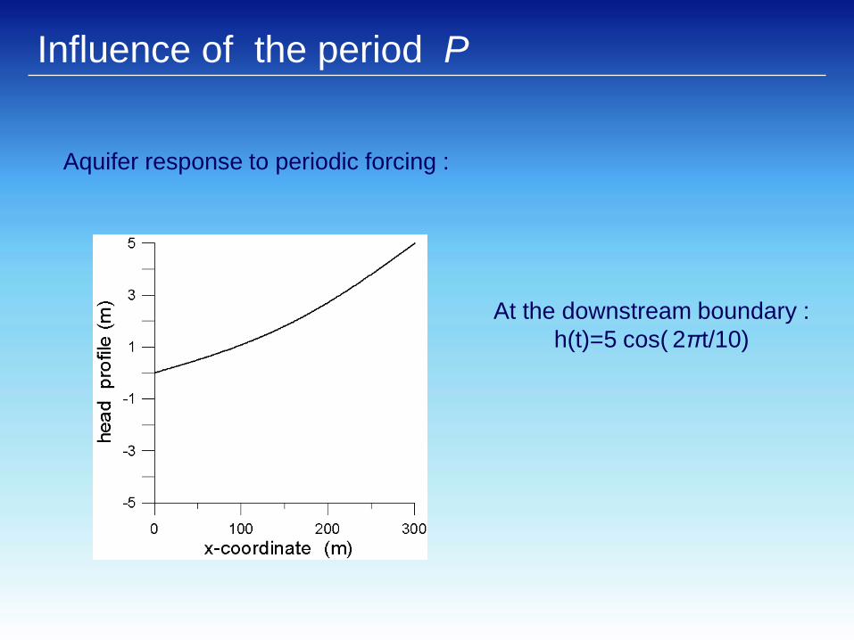
Aquifer response to periodic forcing :

At the downstream boundary :

h(t)=5 cos( 2πt/10)

Head profiles along the aquifer length. The downstream water level is a cosine function with an

amplitude of 5m and with different periods: 1, 5, 10 days. The length of the aquifer is 300m, the

storativity S=0.01.


penetration length l=100m

d/l=1 (aquifer length d=100m)

d/l=3 (aquifer length d=300m)

d/l=6 (aquifer length d=600m) Conclusion

When the period P increases :

• propagation of oscillations increases

• amplitude increases

•d aquifer length

•l penetration length

d/l determine the head profile within the aquifer


Storativity is the ability of the aquifer to store or release water:

For high storativity, the aquifer stores and releases a large

amount of water : fluctuations of the water level will be absorbed

by the porous media.

Influence of the storativity S

water-ΔV

S=ΔA.Δh

Influence of the storativity SS=0.1

S=0.01

S=0.001

S=0.0001

For high storativity : - small amplitude

- delay of the response

- high variations of the velocity near the downstream boundary

steady state

unsteady state S=0.1




Influence of the storativity S

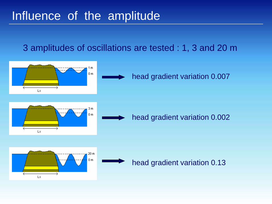
3 amplitudes of oscillations are tested : 1, 3 and 20 m

head gradient variation 0.007



Influence of the amplitude

Small amplitude no significant difference with steady state

Large amplitude oscillations around steady state

Influence of the amplitudesteady state head difference 20m

steady state head difference 3m

steady state head difference 1m

unsteady state amplitude 20m



Spatial distribution of K is modelled as a log-normal distribution.

3 characteristics :

• a mean hydraulic conductivity <K>

• a standard deviation σK

• a correlation length λ

Simulations in heterogeneous aquifers

0 50 100 150 200 250 300

-40

-20

0

1.2

1.6

2

2.4

2.8

3.2

3.6

0 50 100 150 200 250 300

-40

-20

0

0.2

0.8

1.4

2

2.6

3.2

3.8

Map of ln(K)

( arithmetic mean of K =10 m/day and standard deviation σK =5m/day )

λ=2m

λ=40m

0 100 200 300 400Time (days)

0

100

200

300

400

Centr

oid

Dis

pla

cem

ent

in

X-d

irection (

m)

Correlation Length= 1 m(unsteady)



Correlation Length= 1 m (steady)

Correlation Length= 2 m(steady)


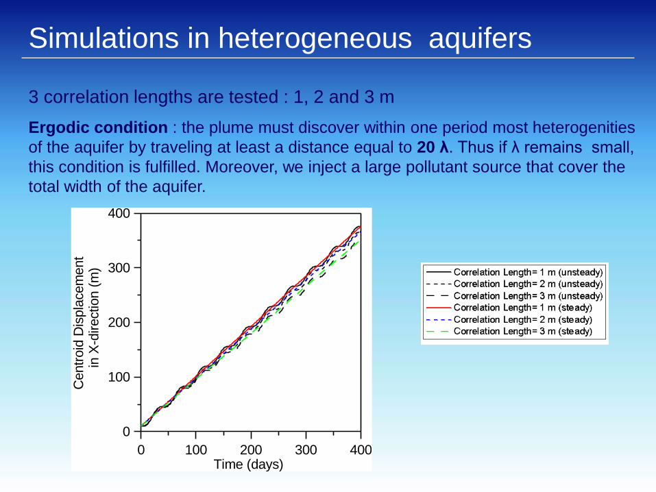
3 correlation lengths are tested : 1, 2 and 3 m

Ergodic condition : the plume must discover within one period most heterogenities

of the aquifer by traveling at least a distance equal to 20 λ. Thus if λ remains small,

this condition is fulfilled. Moreover, we inject a large pollutant source that cover the

total width of the aquifer.


0 100 200 300 400Time (days)

0

100

200

300

400

Variance in X

-direction (

m2)







0 100 200 300 400Time (days)

-2

-1

0

1

2

3

Macro

-dis

pers

ion (

m2/d

ay)

Correlation Length= 1 m (unsteady)






0

0.1

1

10

0 50 100 150 200 250 300 350 400 450 500

-40

-20

0

0 50 100 150 200 250 300 350 400 450 500

-40

-20

0

0 50 100 150 200 250 300 350 400 450 500

-40

-20

0

0 50 100 150 200 250 300 350 400 450 500

-40

-20

0

0 50 100 150 200 250 300 350 400 450 500

-40

-20

0

0 50 100 150 200 250 300 350 400 450 500

-40

-20

0

Correlation Length = 1 m



50 days 150 days 300 days

0 50 100 150 200 250 300 350 400 450 500

-40

-20

0

0 50 100 150 200 250 300 350 400 450 500

-40

-20

0

0 50 100 150 200 250 300 350 400 450 500

-40

-20

0

0 50 100 150 200 250 300 350 400 450 500

-40

-20

0

0 50 100 150 200 250 300 350 400 450 500

-40

-20

0

0 50 100 150 200 250 300 350 400 450 500

-40

-20

0

0 50 100 150 200 250 300 350 400 450 500

-40

-20

0

0 50 100 150 200 250 300 350 400 450 500

-40

-20

0

0 50 100 150 200 250 300 350 400 450 500

-40

-20

0

0 50 100 150 200 250 300 350 400 450 500

-40

-20

0

0 50 100 150 200 250 300 350 400 450 500

-40

-20

0

0 50 100 150 200 250 300 350 400 450 500

-40

-20

0

Steady ConditionsUnsteady Conditions

• Transient case oscillate

around steady state.

• Strong variation in the

plume variance when λ

increases: phenomenon of

channeling appears.


0 50 100 150 200 250 300

-40

-20

0

0 50 100 150 200 250 300

-40

-20

0

0 50 100 150 200 250 300

-40

-20

0

0

5

10

15

20

25

30

35

40

0 10 20 30 40

K

0

0.2

0.4

pd

f

0 10 20 30 40

K

0

0.04

0.08

0.12

pdf

0 10 20 30 40

K

0

0.04

0.08

0.12

pd

f


3 standard deviations are tested : 1, 5 and 10 m/day

when σK increases :

values of K lower than the mean <K> are more probable to

be present in the medium

contrast in K increases

σK=1 m/day

σK=5 m/day

σK=10m/day

heterogeneous aquifer

standard deviation = 1m



0 40 80 120 160

time (days)

0

100

200

300

me

an

d

isp

lace

me

nt in

th

e x

-dir

ectio

n

(m)

0 40 80 120 160

time (days)

0

100

200

300

400

lon

gitu

din

al va

ria

nce

(m2)

0 40 80 120 160

time (days)

170

180

190

200

210

220

230

late

ral va

rian

ce

(m

2)

0 40 80 120 160

time (days)

-2

0

2

4

6

DX

X (

m2/d

ay)

when σK increases :

• Slowing down of the plume

• Enhancement of the

longitudinal spreading

• Enhancement of the lateral

spreading


0 20 40 60 80

time (days)

-8

-4

0

4

8

me

an

dis

pla

ce

me

nt in th

e x

-dir

ectio

n (

m)

xste

ad

y -

xu

nste

ad

y

0 20 40 60 80

time (days)

-8

-4

0

4

8

lon

gitu

din

al va

ria

nce

(m2)

(xx2

s

tea

dy -

(xx2

u

nste

ad

y

0 20 40 60 80

time (days)

-0.8

-0.4

0

0.4

0.8

late

ral v

ari

an

ce

(m

2)

(yy2

s

tea

dy -

(yy2

u

nste

ad

y

0 20 40 60 80

time (days)

-8

-4

0

4

8

me

an

dis

pla

ce

me

nt in t

he

x-d

ire

ctio

n (

m)

xste

ad

y -

xu

nste

ad

y

0 20 40 60 80

time (days)

-8

-4

0

4

8

12

lon

gitu

din

al va

ria

nce

(m2)

(xx2

s

tea

dy -

(xx2

u

nste

ad

y

0 20 40 60 80

time (days)

-2

-1

0

1

2

late

ral v

ari

an

ce

(m

2)

(yy2

s

tea

dy -

(yy2

u

nste

ad

y

0 20 40 60 80

time (days)

0

40

80

120

160lo

ngitudin

al v

ari

ance (

m2)

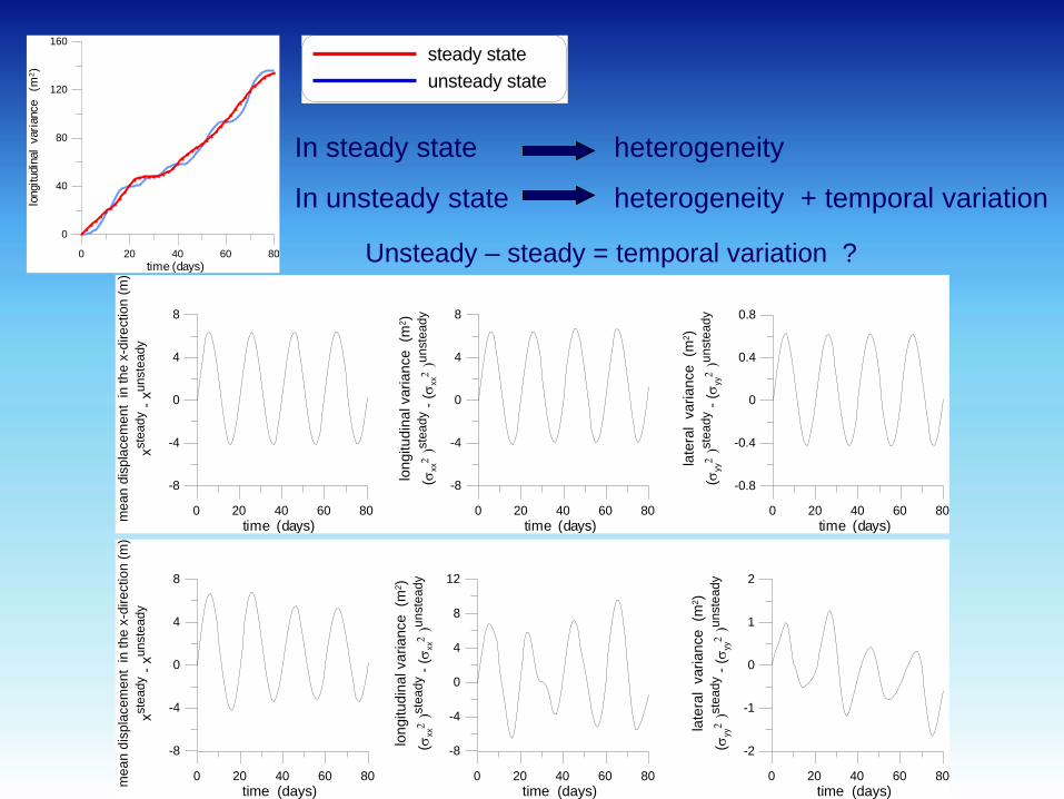
steady state

unsteady state

Unsteady – steady = temporal variation ?

In steady state heterogeneity

In unsteady state heterogeneity + temporal variation

Description of the experiment :

Injection of a non-reactive tracer (bromide) in an real heterogeneous aquifer

Depth-averaged distribution of K

Application to a field tracer test : “ Made1 experiment ’’

Observed concentration and cross-section of K

Description of the field data :

Depth-averaged bromide concentration

Application to a field tracer test : “ Made1 experiment ’’

A lot of uncertainty on:

• the spatial distribution of K

• the values of αL and αT

• the storage coefficient S

Location of the measurements of K

0 50 100 150 200 250 300

-150

-100

-50

0

0

2.5

10

40

70

100

140

180

220

0 20 40 60 80 100 120 140 160

-40

-20

0

0.78

1.3

2

3.5

6

10

16

26

43

71

116

0 50 100 150 200 250-100

-80

-60

-40

-20

0

0

4.3

43

430

injection point

Spatial distribution of K : grid map

where nodes are assigned a value of

K

Case 1. depth averaged map

Case 2. depth averaged map

Case 3. distribution of K at elevation

59m

Data for the numerical simulation

0

50

100

150

200

250

-100-80-60-40-200

62

62.1

62.2

62.3

62.4

62.5

62.6

62.7

62.8

62.9

63

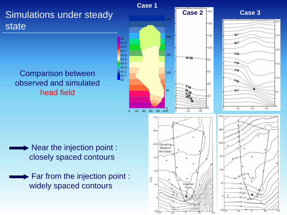
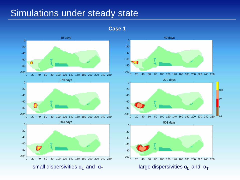
Case 1

Simulations under steady

state

Near the injection point :

closely spaced contours

Far from the injection point :

widely spaced contours

Case 2 Case 3

Comparison between

observed and simulated

head field

Simulations under steady state

Observed concentrations :

Depth-averaged bromide concentration

0 20 40 60 80 100 120 140 160 180 200 220 240 260-100

-80

-60

-40

-20

0

0 20 40 60 80 100 120 140 160 180 200 220 240 260-100

-80

-60

-40

-20

0

0 20 40 60 80 100 120 140 160 180 200 220 240 260-100

-80

-60

-40

-20

0

49 days

279 days

503 days

0 20 40 60 80 100 120 140 160 180 200 220 240 260-100

-80

-60

-40

-20

0

0 20 40 60 80 100 120 140 160 180 200 220 240 260-100

-80

-60

-40

-20

0

0 20 40 60 80 100 120 140 160 180 200 220 240 260-100

-80

-60

-40

-20

0

0.1

1

10

100

49 days

279 days

503 days


Case 1

small dispersivities αL and αT large dispersivities αL and αT

0 20 40 60 80 100 120 140 160-50

-40

-30

-20

-10

0

0 20 40 60 80 100 120 140 160-50

-40

-30

-20

-10

0

0 20 40 60 80 100 120 140 160-50

-40

-30

-20

-10

0

49 days

279 days

503 days

0 20 40 60 80 100 120 140 160-50

-40

-30

-20

-10

0

0 20 40 60 80 100 120 140 160-50

-40

-30

-20

-10

0

0 20 40 60 80 100 120 140 160-50

-40

-30

-20

-10

0

0.1

1

10

100

49 days

279 days

503 days


Case 2


49 days

279 days

503 days

0 50 100 150 200 250 300

-150

-100

-50

0

0 50 100 150 200 250 300

-150

-100

-50

0

0 50 100 150 200 250 300

-150

-100

-50

0

49 days

0 50 100 150 200 250 300

-150

-100

-50

0

0 50 100 150 200 250 300

-150

-100

-50

0

0 50 100 150 200 250 300

-150

-100

-50

0

279 days

503 days

0.1

1

10

100


Case 3


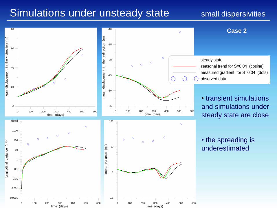
Simulations under unsteady state

1 3 5 7 9 11 13 15 17 19 21 23 25 27 29 31

time (months)

0.001

0.002

0.003

0.004

0.005

gra

die

nt m

agnitude

measured gradient

fitted seasonal component

simulation period

Transient flow conditions :

Fluctuations are imposed at the downstream boundary to recreate the variations of the head gradient

Variation of the hydraulic head gradient magnitude

0 100 200 300 400 500 600

time (days)

-35

-30

-25

-20

-15

-10

me

an

d

isp

lace

me

nt

in

th

e

y-d

ire

ctio

n

(m)

0 100 200 300 400 500 600

time (days)

0.1

1

10

100

late

ral v

aria

nce

(m

2)

0 100 200 300 400 500 600

time (days)

0

20

40

60

80

me

an

dis

pla

ce

men

t in

th

e x

-dir

ectio

n

(m)

0 100 200 300 400 500 600

time (days)

0.0001

0.001

0.01

0.1

1

10

100

1000

10000

lon

gitu

din

al v

ari

an

ce

(m

2)

Simulations under unsteady state small dispersivities

steady state

seasonal trend for S=0.04 (cosine)

measured gradient for S=0.04 (dots)

observed data

• transient simulations

and simulations under

steady state are close

• the spreading is

underestimated

Case 2

0 100 200 300 400 500 600

time (days)

-35

-30

-25

-20

-15

-10

me

an

d

isp

lace

me

nt in

th

e y

-dir

ectio

n

(m)

0 100 200 300 400 500 600

time (days)

10

20

30

40

50

60

me

an

dis

pla

ce

men

t in

th

e x

-dir

ectio

n

(m)

Simulations under unsteady state large dispersivities

steady state



observed data

0 100 200 300 400 500 600

time (days)

0.0001

0.001

0.01

0.1

1

10

100

1000

10000

lon

gitud

ina

l v

ari

an

ce

(m

2)

• transient simulations

and simulations under

steady state are close

• better simulation of

the spreading

0 100 200 300 400 500 600

time (days)

1

10

100

late

ral v

ari

an

ce

(m

2)

Case 2

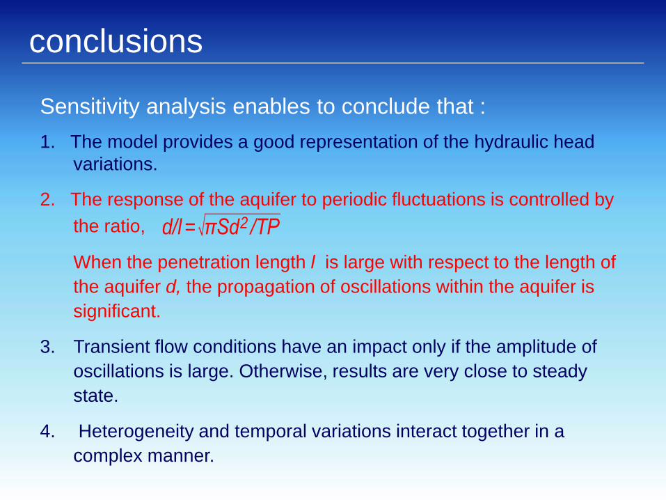
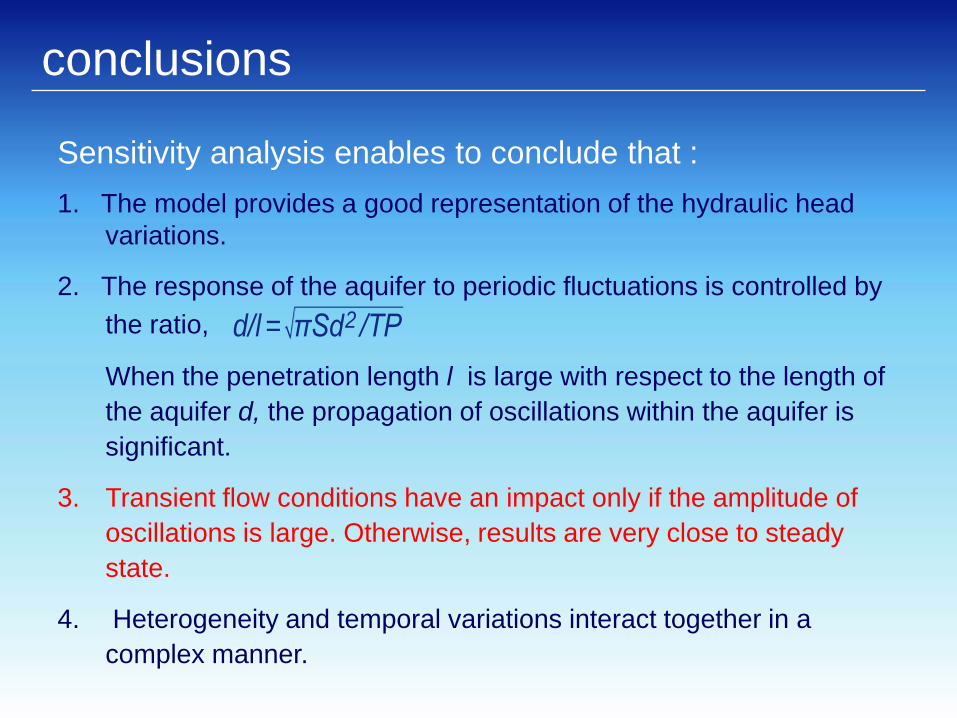
conclusions

Sensitivity analysis enables to conclude that :

1. The model provides a good representation of the hydraulic head

variations.

2. The response of the aquifer to periodic fluctuations is controlled by

the ratio,

When the penetration length l is large with respect to the length of

the aquifer d, the propagation of oscillations within the aquifer is

significant.

3. Transient flow conditions have an impact only if the amplitude of

oscillations is large. Otherwise, results are very close to steady

state.

4. Heterogeneity and temporal variations interact together in a

complex manner.

2d/l = πSd /TP

conclusions

Application to the MADE1 experiment enables to

conclude that :

1. In this example, transient flow conditions don’t show much

difference with steady state conditions

2. The poor agreement between simulated and observed results can

be primarily attributed to uncertainty in the spatial distribution of K:

sparse data and depth-averaged values coarse map

A good knowledge of the geology and thus of the fine-scale

heterogeneity in the aquifer is necessary for simulations

conclusions

Application to the MADE1 experiment enables to conclude

that :

1. In this example, transient flow conditions don’t show much difference

with steady state conditions

2. The poor agreement between simulated and observed results can be

primarily attributed to uncertainty in the spatial distribution of K:

sparse data and depth-averaged values coarse map

A good knowledge of the geology and thus of the fine-scale

heterogeneity in the aquifer is necessary for simulations

Annexes

1 1

1 1

cos sin sin cos

. / . / . / . /

n n n np p x p p yL T L T

n n n np p x x y p p y y xL T L T

X X V t Z Z Y Y V t Z Z

X X V t Z V V Z V V Y Y V t Z V V Z V V

6 4 4 4 44 7 4 4 4 4 486 7 8dispersive termadvective term

1 22 2xy yxx x

p p x L T

D VD VX t t X t V t Z V t Z V t

x y V V

1 22 2yx yy y x

p p y L T

D D V VY t t Y t V t Z V t Z V t

x y V V

The displacement is a normally distributed random variable, whose

mean is the advective movement and whose deviation from the mean

is the dispersive movement.

instantaneous injection

+ uniform flow

Annexes

“Courant condition” :

The distance traveled by a particle in one step must not exceed the size of thecells: thus particles don’t jump over cells, and move continuously from one cell toanother.

trans

max

ΔxΔtV

Time discretization of flow and transport

x x xt t t1 2 2 2 1V t =V t 1-A +V t A with A = t-t / t -t

Annexes

dtflow=10 days dttrans=10 days (no interpolation)

dtflow=10 days dttrans= 5 days ( interpolation)

dtflow=10 days dttrans= 1 days ( interpolation)

dtflow= 5 days dttrans= 5 days (no interpolation)

dtflow= 1 days dttrans= 1 days (no interpolation)

Annexes

0 100 200 300 400 500 600

time (days)

-114

-112

-110

-108

-106

-104

me

an

d

isp

lace

me

nt in

y-d

ire

ctio

n

(m)

0 100 200 300 400 500 600

time (days)

1

10

100

late

ral v

aria

nce

(m

2)

Case 3

steady state




observed data

0 100 200 300 400 500 600

time (days)

60

64

68

72

76

80

me

an

d

isp

lace

men

t in

x-d

ire

ctio

n

(m)

0 100 200 300 400 500 600

time (days)

0.001

0.01

0.1

1

10

100

1000

10000

lon

gitud

ina

l v

ari

an

ce

(m

2)

small dispersivities

Annexes

Case 3

large dispersivities

0 100 200 300 400 500 600

time (days)

-116

-114

-112

-110

-108

-106

-104

me

an

d

isp

lace

me

nt in

y-d

ire

ctio

n

(m)

steady state




observed data

0 100 200 300 400 500 600

time (days)

1

10

100

late

ral v

aria

nce

(m

2)

0 100 200 300 400 500 600

time (days)

60

64

68

72

76

80

me

an

d

isp

lace

men

t in

x-d

ire

ctio

n

(m)

0 100 200 300 400 500 600

time (days)

0.001

0.01

0.1

1

10

100

1000

10000

lon

gitu

din

al v

ari

an

ce

(m

2)

head at x=50m

head at x=100m

head at x=150m

head at x=200m

velocity at x=50m

velocity at x=100m

velocity at x=150m

Annexes

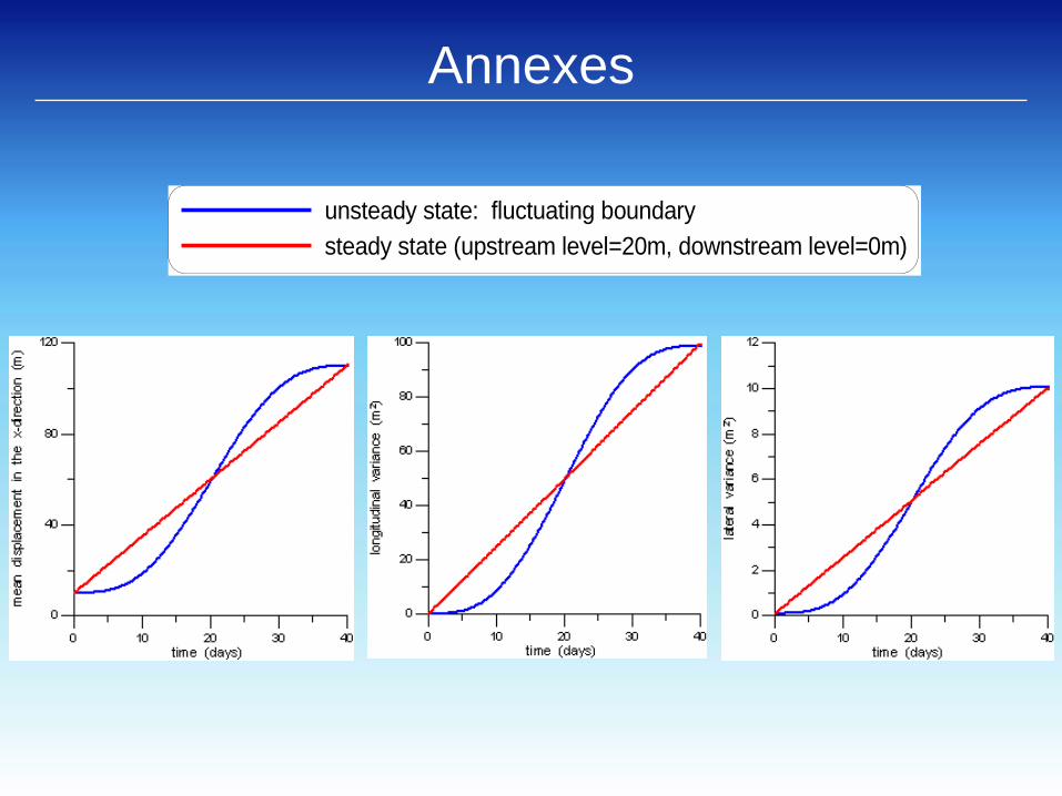
unsteady state: fluctuating boundary

steady state (upstream level=20m, downstream level=0m)

Annexes

modeling dispersion under unsteady groundwater flow conditions

Engineering