modeling dynamic redemption and default risk for lbo...

Modeling Dynamic Redemption and Default Risk forLBO Evaluation: A Boundary Crossing Approach

Abstract

We analyze corporate financial policies in leveraged buyouts (LBOs) in the pres-

ence of default risk. Our model captures the LBO-specific stepwise debt reduc-

tion, either with predetermined or cash-flow dependent (cash sweep) principal

payments, and thus allows for dynamic redemption. These dynamics imply

stochastic, discontinuous default boundaries. Our framework enables us to de-

rive explicit-form solutions for the net present value (NPV ) and the internal

rate of return (IRR) of an LBO investment. We show that in scenarios with

high entry debt and high redemption payments, the flexibility associated with

dynamic redemptions creates value for investors, while fixed redemptions yield

higher NPV and IRR values for moderate redemption due to lower debt yields.

Moreover, we discuss optimal corporate financial policies implied by NPV or

IRR maximization and find that the latter always results in increased leverage

with higher default probability. The model of piecewise linear boundaries de-

veloped in this article is sufficiently flexible to be applied to a wide range of

problems in corporate finance.

Keywords: Default at first passage, Dynamic redemption, Barrier options,

Brownian motion, Numerical integration, Leveraged buyouts

JEL classification: C61, C63, G12, G13, G32, G33

Preprint submitted to Elsevier January 7, 2016

1. Introduction

Leveraged buyouts (LBOs) are a specific type of corporate transaction in

which the buyer, often private equity (PE) funds, acquires a target company for

a limited holding period (on average, three to five years, see, e.g., Kaplan and

Stromberg, 2008). In particular, after entry, the buyer imposes a new capital

structure onto the target; this structure is characterized by a small portion of

equity and a significant portion of debt (Axelson et al., 2013, find that LBO-

backed firms have a debt-to-enterprise value ratio that is twice as high as that

of their industry peers). The target firm reduces this initial debt level in a

stepwise manner over the holding period, either by contractually fixed principal

payments or by a redemption schedule that depends on the target firms’ gener-

ated cash flows (the so called “cash sweep” redemption). As these observations

suggest, LBOs are characterized by a different capital structure and redemp-

tion policy than their industry peers (e.g., Axelson et al., 2013). Our article

examines the dynamics of financial policies in an LBO setting and their link to

investment decisions. By accounting for the aforementioned characteristics, we

provide explicit-form solutions for pricing LBO investments and quantitative

explanations for those solutions.

Discussions between critics and proponents of the role of debt in LBO trans-

actions are heated. On the one hand, proponents note that the extensive use

of debt creates interest tax shields, efficiency gains (e.g., Berg and Gottschalg,

2005) and lower agency costs due to the disciplining effect of debt (Jensen and

Meckling, 1976). On the other hand, critics claim that extensive debt usage in

LBO transactions exposes the target firm to high bankruptcy risks1 while the

PE fund reaps unjustifiably high tax savings (e.g., Rasmussen, 2009). Although

the subject of several empirical studies, this discrepancy puzzles theorists con-

cerned with the effect of a firm’s financing policy.

As the transaction volume of LBOs in 2007 of approximately $1.6 trillion

demonstrates (Kaplan and Stromberg, 2008), it is highly economically relevant

1Tykvova and Borell (2012) find no evidence that the bankruptcy rates of PE-owned firmsdiffer from those of their peers. In contrast, Hotchkiss et al. (2014) find a higher bankruptcyprobability. Stromberg (2007) finds that approximately 6% of the PE target firms in hissample default; however, his study does not cover the effects of the financial crisis.

2

to identify a pricing mechanism that captures the specifics of an LBO. Therefore,

the aim of this paper is to address the aforementioned challenges. We develop

a model to analyze the financial effects of an LBO based upon a boundary-

crossing approach. Our model explicitly reflects upon default risk and captures

the particular feature of dynamic (cash-flow dependent) debt redemption. By

introducing piecewise discontinuous boundaries into this classical real options

application, we are able to provide explicit-form solutions that allow us to as-

sess an LBO based on the NPV and IRR investment criteria. This approach

provides the opportunity to determine important value drivers, such as the tax

shield. Moreover, by maximizing either NPV or IRR, we find the optimal capital

structure and redemption policy of an LBO. Thus, we are able to compare and

critically discuss the impact of the investment criteria on optimal debt levels in

a dynamic framework.

We may know the economic rationales motivating PE investors to impose

an LBO-specific debt structure (e.g., tax shield generation, IRR maximization),

but existing models quantifying the value impact of debt do not fully capture all

LBO-related aspects. A well established body of literature discusses the impact

of different “financing policies”, i.e., strategies of redeeming debt, taking on

new debt and adapting the level of debt to changes in economic conditions (e.g.,

Myers, 1974; Miles and Ezzell, 1980; Cooper and Nyborg, 2010). These financing

policies drive the risk properties of future debt levels and, by doing so, the risk

of the tax savings attached to them. None of the established models account for

the debt dynamics in LBOs: On the one hand, as first proposed by Myers (1974),

a financing policy with state-independent absolute debt levels does not properly

capture the “cash sweep” (path-dependent) redemption dynamics. On the other

hand, the policy of Miles and Ezzell (1980) assuming that firms regularly adjust

the level of outstanding debt to changes in firm value by adopting a state-

independent leverage ratio is unable to model a stepwise redemption.

Moreover, the financing policy of LBOs also stands in stark contrast to es-

tablished models of the optimal capital structure, “trading-off” the benefits and

costs of debt. Most trade-off models assume a perpetual setting and derive an

3

optimal debt level to be permanently maintained2. Instead, the financing pol-

icy of LBOs is characterized by high entry debt levels and flexible redemption

over the course of a limited holding period. Existing capital structure models

(e.g., Leland, 1994; Goldstein et al., 2001) consider a console bond or dynami-

cally adjust the debt issue proportional to the asset value. To find the optimal

debt level, a certain continuous threshold triggering bankruptcy is determined

endogenously. The critical implication of this approach is that redemption pay-

ments are either not directly mapped or move proportional to the asset value.

Thus, existing dynamic models of the optimal capital structure choice are un-

able to capture the empirically observed financing policies in LBOs and need to

be extended (Axelson et al., 2013).

Some models, however, try to overcome the described shortcomings and

to account for the LBO-specific debt dynamics: Arzac (1996) provides two

potential solutions, a recursive APV and a European call option approach. The

recursive APV approach still yields significant valuation errors as the valuation

of the debt-related tax benefits requires a known discount rate. The option

approach addresses this challenge but requires another simplifying assumption:

The firm can only default on its debt at the due date which is equal to the end

of the holding period. Other models allow for potential default over the entire

lifetime of the debt contract: Couch et al. (2012) use a barrier option approach

to value debt-related tax savings in an LBO setting. Default is triggered by

the EBIT hitting a lower constant barrier reflecting an interest coverage ratio.

An extended version allows for one-time refinancing over the infinite lifetime of

the firm. Braun et al. (2011) also use a barrier option approach allowing for

default over the entire lifetime of the debt contract in LBOs. Default occurs

when the firm value drops below the face value of debt. In this approach,

the future debt levels serving as lower barrier are assumed to be certain and

described by an exponentially declining function. While both models allow

for default over the entire lifetime of the debt contract, they still do not fully

reflect upon the redemption policies typically employed in LBOs: First, a fixed

2As empirical studies on the speed of adjustment (e.g., Flannery and Rangan, 2006)suggest, the capital structure of public firms fluctuates around a certain (optimal) targetlevel.

4

and stepwise redemption of debt requires a stepwise adjustment of the default

barrier, imposing technical problems due to the non-differentiable nature of the

barrier. Second, the “cash sweep” (dynamic) redemption policy necessitates

multiple path-dependent adjustments of the default barrier.

We contribute to this literature stream by developing a model flexible enough

to incorporate redemption policies with either fixed, stepwise repayments or

dynamic, path-dependent repayments. In addition, high debt levels are an ob-

vious characteristic of LBOs, consequently, the risk of default is specifically

important. We introduce a boundary-crossing approach to map complex de-

fault triggers implied by the LBO-specific redemption policies. The mechanics

are equivalent to a down-and-out barrier option with rebate. Default occurs ei-

ther if a cash obligation consisting of repayment plus interest (fixed redemption)

or a cash-flow-dependent covenant, e.g., a given maximum interest coverage or

debt-to-EBITDA ratio, is hit within the holding period. Existing barrier option

models (e.g., Merton, 1973; Cox and Rubinstein, 1985; Kunitomo and Ikeda,

1992; Roberts and Shortland, 1997; Lo et al., 2003) require boundaries that

follow a certain differentiable function. Due to the dynamic, path-dependent

redemption policy, debt becomes a path-dependent variable, and in turn, the

default trigger is also path-dependent. This type of trigger is difficult to imple-

ment because the stochastic boundary is subject to stepwise changes, i.e., the

boundary does not have a differentiable functional form. In brief, the existing

barrier option models cannot be used to capture the aforementioned dynam-

ics. Hence, we apply the basic idea of Wang and Potzelberger (1997) by using

piecewise linear boundaries. This approach offers the opportunity to model any

type of boundary, including discontinuous ones. Wang and Potzelberger (2007)

extend their early approach to allow for an application to geometric Brownian

motions (gBm). Based on this work, our model equations are in explicit form:

To solve for complex default boundaries, numerical integration is required. (3.)

Additionally, our analysis also endogenizes the pricing of debt. Based on the

boundary-crossing approach, we derive the promised yield of debt resulting in

NPV-neutral debt contracts. As credit risk premia of leveraged loans have been

shown to be an important factor in LBO leverage choices (Axelson et al., 2013)

our model captures this important feature.

5

Beyond the aforementioned contribution to pricing techniques, our model

accounts for two additional important characteristics of LBOs. First, Colla

et al. (2012) demonstrate that firm-specific drivers such as operating perfor-

mance (EBIT) and volatility are important determinants of leverage choices

in LBOs. We include these variables by assuming a stochastic EBIT process

following a gBm and allowing for changes in drift and standard deviation. Sec-

ond, PE sponsors in particular steer target companies based on the IRR of

their investment rather than on its net present value (NPV) (see, e.g., Kaplan

and Schoar, 2005). In other words, PE investors may choose an LBO capital

structure based on a completely different rationale, as standard trade-off frame-

works suggest. To provide an example, consider the optimal capital structure

choice in the prominent trade-off model of Leland (1994) where the objective

is to maximize the equity value. The equityholders’ endogenous choice of the

bankruptcy trigger directly implies the optimal debt level. In the most simple

terms, given an already fixed investment outlay, the optimal capital structure

choice in these models rests upon the NPV criterion. As our model framework

allows for inversion, we are able to determine the IRR for any capital structure

chosen by the investor and, thus, to identify the one maximizing the IRR. Using

both investment criteria in a dynamic model enables critical reflection on the

IRR beyond the well-known arguments.3

We find that optimizing an LBO debt structure based on the IRR in general

results in higher leverage, increased default risk, and a lower value creation than

optimization based on the NPV. Moreover, we provide an economic rationale

for the existence of fixed and cash sweep debt contracts in LBOs. Cash sweep

debt redemption generates equity-like payoffs to debtholders, because redemp-

tion varies with interest-exceeding stochastic cash flows. Thus, debtholders

demand a risk premium within their promised yield. On the opposite side, flex-

ible debt repayments reduce the risk to technically default which increases the

3Lorie and Savage (1949) and Hirshleifer (1958) revealed a number of difficulties of the IRR,thereby shaping subsequent academic opinion. The very special reinvestment assumption, thepossibility of multiple results, the possibility of making an incorrect investment decision formutually exclusive projects, and the difficulty of applying the IRR rule when the cost ofcapital varies over time are the four main pitfalls in the classical literature. Brealey andMyers (and subsequently Allen) summarized these issues in their famous textbook “Principlesof Corporate Finance.” The first edition was released in 1980, and their arguments haveremained unchanged through the most recent version (Brealey et al., 2013).

6

expected future free cash flows to firm. This trade-off determines which of the

two redemption policies is favorable. Given a moderate financing policy with

low default probability, fixed debt redemption is value-creating for equityholders

caused by a lower promised yield of debt. Cash sweep debt redemption creates

value under riskier financing policies, because a comparable fixed redemption,

forcing high cash obligations, implies a significantly higher risk of default.

The remainder of the paper is organized as follows. Section 2 introduces the

model, with Section 2.1 stating the basic assumptions, Section 2.2 illustrating

the specific debt structure, Section 2.3 defining the default triggers, Section 2.4

deriving the payoff components, Section 2.5 introducing the investment crite-

ria, and Section 2.6 elaborating on the pricing of debt. Section 3 presents the

stochastics of the model and shows the explicit analytic-form solution for some

special cases and the explicit integral form solution for the general case. In

Section 4, we use the stochastic attributes derived to develop solution formulae

for all NPV and IRR components. Section 5 illustrates the results through a

numerical application and provides comparative statics. Section 6 concludes the

paper.

2. The setting

2.1. Basics of the model

Table 1 provides a notation index. Our assumptions concerning the nature

of uncertainty are standard. Let (Ω, F , P, (Ft)t≥0) be a complete probability

space supporting a standard Brownian motion Wt and [0, T ] a time interval,

where T → ∞ is possible. We denote the available information at time t,

with t ∈ [0, T ], by the filtration Ft ⊂ F where Ft describes the augmented

σ-algebra generated by the standard Brownian motion. We assume a market

without arbitrage opportunities. For each subjective probability measure P,

there exists an equivalent measure Q called the risk-neutral probability measure.

We denote the expected value operator by E(.) and use the subscript to indicate

the respective probability measure. In the subsequent analysis, we pursue a

risk-neutral pricing approach.

Consider a levered firm, the value of which at time t is given by V Lt . Ac-

cording to Modigliani and Miller (1963), the value of the levered firm can be

7

Table 1: Notation index. This table summarizes all notations applied within the paper cate-gorized by input parameters (upper-left), model output (upper-right) and stochastic notation(lower-left).

Input parameters Model output

Variable Description Variable Description

T holding period in years cot cash obligation against debtholders in tEBIT t earnings before interests and taxes in t dst total debt service in tτc corporate tax rate dbt default boundary in tXt unlevered after-tax cash flow in t XCt excess cash in tµP drift rate of EBIT I0 initial investment in t = 0µ risk-neutral drift rate of EBIT POt payoff in tσ volatility of EBIT PVPO present value of a payoffr risk-free rate V Lt value of the levered firm in trA asset rate V Ut value of the unlevered firm in tλ market price of risk V TSt value of the tax shield in tbp input parameter for PH PH contingent present value factor for V TSt

a input parameter for PH pdt,Q probability of default in tyD promised yield of debt cdt,Q cumulative probability of default up to tDt debt level of the target company in t NPV net present valuel∗ industry avg. multiple for debt after exit IRR internal rate of returnγ cash sweep redemption ratio Ct interest payment in tθ dividend ratio Rt debt redemption in tβ debt-to-EBIT covenant PODht payoff to debtholders in tρ bankruptcy cost ratio NPV Dh net present value for debtholders

Stochastic notation

Variable Description

t arbitrary point in timed point in time of defaultP subjective real-world probability measureQ risk-neutral probability measureEP expected value under PEQ expected value under QF filtrationΩ probability space1 indicator functionN cumulative normal distribution functionWt standard Brownian motion in period tMt minimum of standard Brownian motion up to tα drift rate of Brownian motionm lower constant boundary to Brownian motion

8

determined by adding the present value of the tax savings from interest pay-

ments on debt V TSt to the value of an otherwise identical but unlevered firm

V Ut . The corporate tax rate τc, and the risk-free rate r are assumed to be

deterministic and constant. We do not consider personal taxes.

The operations of the firm generate an uncertain income. Similar to several

representatives of the corporate finance theory literature (e.g., Hackbarth et al.,

2007), our measure of income is the earnings before interest and taxes EBIT of

a nondepreciating machine with a mean return µP. Neither an income metric

nor a cash flow are typically traded assets. Thus, we do not assume EBIT to

be spanned. Instead, we introduce a spanning portfolio Y with a mean return

rA and a volatility σ that is equal to the volatility of EBIT . As the risk of

EBIT contains an idiosyncratic component, rA > µP holds. The evolutions of

EBIT and Y are as follows:

dEBIT

EBIT=µPdt+ σdWt (1)

dY

Y=rAdt+ σdWt. (2)

For Y , the risk-neutral mean return is r due to the spanning property. Thus,

we have rA−λσ = r, where λ is the market price of risk. Rearranging this term

results in:

λ =rA − rσ

. (3)

With (3) at hand, we find the risk-neutral drift of EBIT which we denote

by µ:

µ =µP − λσ

=µP − (rA − r). (4)

We retain the typical Modigliani and Miller assumption that EBIT is in-

dependent of the pursued debt policy. To conclude, EBITt follows a geometric

Brownian motion (gBm) under the risk-neutral probability measure Q with an

initial value of EBIT0 > 0 given by:

dEBITt = µEBITtdt+ σEBITtdWt, (5)

9

where µ is the constant risk-neutral drift rate, σ the constant standard de-

viation of the EBIT and Wt a standard Brownian motion.

The income process also drives the free cash flow to firms in our model,

which we denote by X. For simplicity, we assume that EBIT less corporate

taxes allows us to arrive at X4:

Xt =EBITt(1− τc). (6)

The firm’s debt is subject to the risk of default. The firm pays interest

and redemption on the outstanding total amount of debt Dt. The credit risk-

adjusted yield of debt is denoted by yD. This promised yield is determined

endogenously under the assumption that debtholders claim an interest rate that

yields an NPV of zero for the debt contract.5

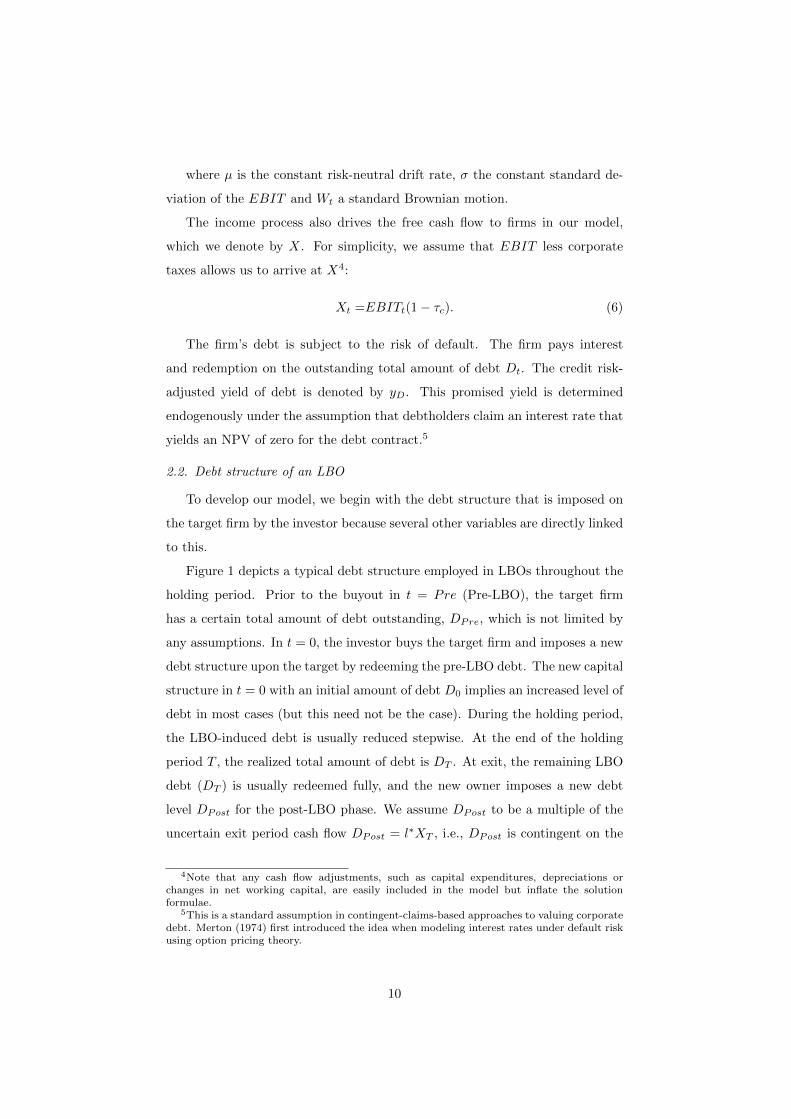
2.2. Debt structure of an LBO

To develop our model, we begin with the debt structure that is imposed on

the target firm by the investor because several other variables are directly linked

to this.

Figure 1 depicts a typical debt structure employed in LBOs throughout the

holding period. Prior to the buyout in t = Pre (Pre-LBO), the target firm

has a certain total amount of debt outstanding, DPre, which is not limited by

any assumptions. In t = 0, the investor buys the target firm and imposes a new

debt structure upon the target by redeeming the pre-LBO debt. The new capital

structure in t = 0 with an initial amount of debt D0 implies an increased level of

debt in most cases (but this need not be the case). During the holding period,

the LBO-induced debt is usually reduced stepwise. At the end of the holding

period T , the realized total amount of debt is DT . At exit, the remaining LBO

debt (DT ) is usually redeemed fully, and the new owner imposes a new debt

level DPost for the post-LBO phase. We assume DPost to be a multiple of the

uncertain exit period cash flow DPost = l∗XT , i.e., DPost is contingent on the

4Note that any cash flow adjustments, such as capital expenditures, depreciations orchanges in net working capital, are easily included in the model but inflate the solutionformulae.

5This is a standard assumption in contingent-claims-based approaches to valuing corporatedebt. Merton (1974) first introduced the idea when modeling interest rates under default riskusing option pricing theory.

10

state of the firm in T . The leverage ratio l∗, with l∗ ≥ 0, can be, e.g., regarded

as a sustainable industry average. While we introduce this assumption to ensure

a state-dependent exit price, it is not critical to the model. Our approach also

works with any other assumption concerning DPost.

3

Entry & Refinance

Exit & Refinance

…

Pre-LBO Holding Period

Fixed:Cash Sweep: min , · max 1 , 0

Figure 1: Basic structure of debt redemption in an LBO. The investor imposes a new,increased debt level D0 at entry (t = 0). During the holding period, the acquired firmpartially repays the increased debt to arrive at DT , which may be higher than, lower than orequal to the new post-exit debt level DPost. DPost depends on the state of the firm in T .

We analyze two major redemption policies popular in LBOs: fixed and cash

sweep repayment. Irrespective of the case, we denote debt redemption with

R(.)t . In the fixed case, there is a predetermined redemption ft at each time

point t during the holding period. In contrast, cash sweep redemption describes

is flexible: A proportion γ, with γ ∈ [0, 1], of the firm’s realized free cash flow

Xt increased by the tax savings, yDτcDt−1, and reduced by interest payments,

yDDt−1 is repayed.6 Considering the specific structures of the redemption cases

6For simplicity, we assume γ to be a constant parameter. Note that a time-dependent γtcan easily be incorporated into the model.

11

yields:

Rfixedt = ft, (7)

Rsweept = min (Dt−1, γmax (Xt − yDDt−1(1− τc), 0)) . (8)

The min-max combination in Equation (8) is necessary to account for the

specific flexibility of cash sweep debt redemption. The max condition prevents

new debt from being added if Xt is not sufficient to serve the after-tax interest

payments yDDt−1(1 − τc). The min condition restricts Dt−1 to be positive

(Dt−1 ≥ 0), i.e., if γ(Xt − yDDt−1(1− τc)) exceeds the outstanding debt, only

Dt−1 will be redeemed (non-negative condition).

Hence, the firm’s future debt level at an arbitrary time t is determined by:

D(.)t = D0 −

t∑s=1

R(.)s (9)

for both redemption policies.

The total debt service ds(.)t at an arbitrary point in time t equals the sum

over redemption R(.)t and after-tax interest payments NC

(.)t . Therefore, we

obtain the following congruent definition:

ds(.)t = NC

(.)t +R

(.)t , (10)

where Equations (7) to (8) specify R(.)t , and where NC

(.)t is described by:

NC(.)t = yDDt−1(1− τc). (11)

.

2.3. Default in an LBO

In our model, default is triggered if our unlevered after-tax cash flow X

becomes sufficiently low and hits the default boundary from above. In the liter-

ature regarding (the optimal choice of) debt financing two contrasting economic

mechanisms are usually considered to determine the default boundary (Strebu-

laev and Whited, 2011). Most existing models endogenously determine the

optimal default threshold by maximizing the equity value (e.g., Leland, 1994;

Goldstein et al., 2001). Usually, the aforementioned boundary is a certain asset

value (e.g., Leland, 1994). Such an endogenously chosen default trigger implic-

12

itly assumes equityholders to have deep pockets, i.e., they always prevent illiq-

uidity by covering coupon payments if needed (Strebulaev and Whited, 2011).

However, the implied “deep pocket” assumption does not generally hold for eq-

uityholders in LBO transactions as they are often closed PE funds with a fixed

fund size which is fully distributed to promising investments. Therefore, as dis-

cussed by Achleitner et al. (2012), debtholders should not expect PE investors

to prevent a default by injecting additional equity.

Others consider a flow-based, exogenous threshold (e.g., Kim et al., 1993).

We apply this second economic mechanism where we trigger default by illiquidity

or a covenant violation. The so-called exogenous default trigger is appropriate

for our model for three reasons. Firstly, as outlined in the previous section,

high initial debt levels are redeemed stepwise over the holding period gener-

ating significant cash obligations. Thus, the risk of illiquidity is outstanding

compared to the aforementioned excessive indebtedness argument (Achleitner

et al., 2012). Secondly, debt contracts of LBOs comprise a variety of covenants.

For instance, Achleitner et al. (2012) find a significantly higher number of fi-

nancial covenants in PE-sponsored debt contracts in contrast to non-sponsored

debt contracts. Almost every (97%) sponsored loan includes a combination of

a debt-to-EBITDA and a cash flow coverage covenant. Thirdly, redemption

policies in LBOs, particularly cash-sweep redemption, demand discontinuous,

path-dependent default boundaries rather than one continuous, fixed default

trigger (e.g., Goldstein et al., 2001).

In the absence of a covenant, default is triggered if the realized cash flows

Xt plus any available excess cash accumulated before time point t, XCt−1, do

not cover the cash obligations cot. Under fixed redemption, cash obligation and

debt service are identical (dsfixedt = cofixedt ), while in the cash sweep case, the

cash obligation is limited to the after-tax interest payments:

cofixedt = NCfixedt +Rfixedt , (12)

cosweept = NCsweept . (13)

Excess cash XCt is the sum of previous period’s excess cash up to time t−1,

invested at the risk-free rate r for one period plus the retained share of the net

cash flow (1 − θ)(Xt − cot) in t. The parameter θ, with θ ∈ [0, 1], denotes

13

the dividend ratio established by the investor.7 Occasionally, θ is restricted in

LBOs through debt contracts to foster the excess cash account, which creates

a cushion against default and shields the debtholders. Summarizing, the excess

cash XCt is determined by:

XCt = XCt−1er(1−τc) + (1− θ) (Xt − cot) . (14)

Moreover, debt contracts usually contain certain minimum requirements,

called covenants, for a specific income or cash flow metric. A typical covenant is

a ratio β of debt-to-EBIT or debt-to-EBITDA.8 While we apply debt-to-EBIT

((Dt−1−XCt−1)/EBITt ≤ β), the model allows for any other common covenant

related to debt, interest and performance measures. Note that we consider net

debt (Dt−1−XCt−1) for the covenant condition, as excess cash can be regarded

as negative debt.

Independent of the redemption policy considered, default of the target firm

is triggered if cash flow plus excess cash are not sufficient to cover the firm’s cash

obligation or if the covenant condition is no longer fulfilled. We rearrange both

conditions for Xt and formulate a general rule for default and going concern in

our model:

Default (def):(Xt < co

(.)t −XCt−1er(1−τc)

)∪(Xt <

Dt−1 −XCt−1β

(1− τc)),

for ∃ 0 < t ≤ T. (15)

Going concern (gc):(Xt ≥ co(.)t −XCt−1er

)∪(Xt ≥

Dt−1 −XCt−1β

(1− τc)),

for ∀ 0 < t ≤ T. (16)

Based on condition (15), we can derive a (lower) default boundary to thecash flow Xt. Mechanically, we determine the default boundary at time t − 1

for the subsequent period up to t and denote it by db(.)t . These path-dependent

7For simplicity, we assume θ to be a constant parameter. Note that a time-dependent θtcan easily be incorporated into the model.

8For simplicity, we assume β to be a constant parameter. Note that a time-dependent βtcan easily be incorporated into the model.

14

boundaries are defined for our two redemption cases in the following way:

db(.)t = max

(co

(.)t −XCt−1e

r(1−τc),Dt−1 −XCt−1

β(1− τc)

), for [t− 1, t]. (17)

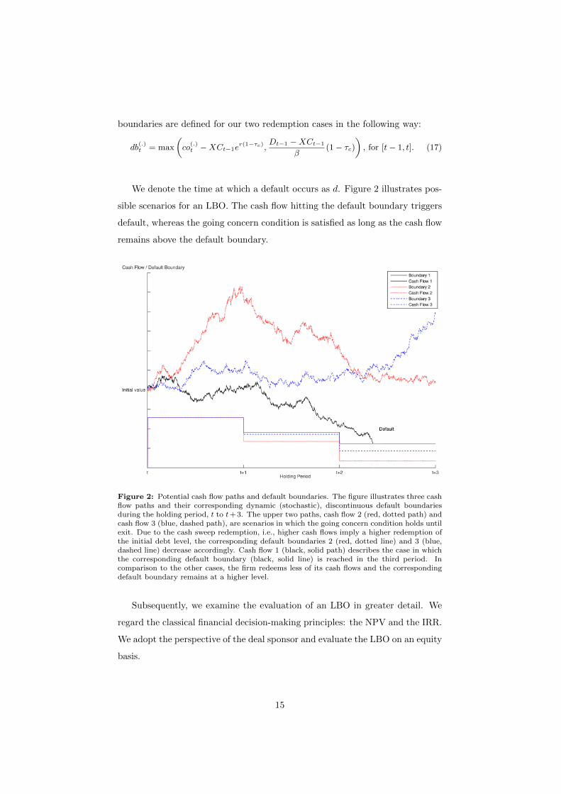
We denote the time at which a default occurs as d. Figure 2 illustrates pos-

sible scenarios for an LBO. The cash flow hitting the default boundary triggers

default, whereas the going concern condition is satisfied as long as the cash flow

remains above the default boundary.

Figure 2: Potential cash flow paths and default boundaries. The figure illustrates three cashflow paths and their corresponding dynamic (stochastic), discontinuous default boundariesduring the holding period, t to t+ 3. The upper two paths, cash flow 2 (red, dotted path) andcash flow 3 (blue, dashed path), are scenarios in which the going concern condition holds untilexit. Due to the cash sweep redemption, i.e., higher cash flows imply a higher redemption ofthe initial debt level, the corresponding default boundaries 2 (red, dotted line) and 3 (blue,dashed line) decrease accordingly. Cash flow 1 (black, solid path) describes the case in whichthe corresponding default boundary (black, solid line) is reached in the third period. Incomparison to the other cases, the firm redeems less of its cash flows and the correspondingdefault boundary remains at a higher level.

Subsequently, we examine the evaluation of an LBO in greater detail. We

regard the classical financial decision-making principles: the NPV and the IRR.

We adopt the perspective of the deal sponsor and evaluate the LBO on an equity

basis.

15

2.4. Payoff structure of an LBO

An LBO generates three different types of payoffs distinguished by the time

of their occurrence: the initial investment I0 to purchase the target, the equity

cash flows POHP at an arbitrary point in time during the holding period, and

the exit equity value POExit from selling the target company.

The initial equity investment I0 at time t = 0 is equal to the enterprise

deal value V L0 minus the entry debt D0. The enterprise deal value is the sum

of the unlevered firm value, V U0 , and the tax shield value, V TS0 . We define

V U0 simply as a perpetuity depending on the current EBIT level EBIT0, the

existing corporate tax rate τc, the risk-free rate r, and the risk-neutral drift

of the EBIT-process µpre prior to the LBO. To price V TS0 , we follow Couch

et al. (2012) as this approach resonates well with our basic idea of a default

boundary defined by a covenant. The basic assumption is that the firm holds

DPre constant and earns interest tax savings of (yD,PreDPreτc) in each period.

These tax savings are subject to default risk, and the bankruptcy trigger is a

constant barrier determined by a covenant, which is related to the stochastic

EBIT process. While Couch et al. (2012) use an interest coverage ratio, we

continue to apply our debt-to-EBIT covenant. By constructing a perpetual,

down-and-in, cash-at-hit-or-nothing, single-barrier option that pays one dollar

when the underlying, X = EBIT (1− τc), hits the barrier, (1− τc)(D−XC)/β,

and zero otherwise, one arrives at a ”contingent present value factor for the

random time when the underlying hits the barrier from above” (Couch et al.,

2012, p. 127). The valuation formula for such an option PH is stated in Equation

(21) with parameters bp and a defined in Equations (22) and (23). A complete

derivation of the option’s valuation formula is provided in Rubinstein and Reiner

(1991).

V U0 = X01

r − µpre, (18)

V TS0 =yD,PreDPreτc

r(1− PH,pre), (19)

I0 = V U0 + V TS0 −D0, (20)

16

with

PH,pre =

( Dt−1−XCt−1

β (1− τc)X0

)bp,pre, (21)

bp,pre = apre +

√a2pre + 2

r

σ2, (22)

apre =µpreσ2− 1

2. (23)

While extensions to the derivation of I0, e.g., a bid premium or expected

costs of financial distress, can easily be incorporated into the model, our defini-

tion is sufficient to endogenize the initial investment.

The equity cash flows as payoffs over the holding period depend on whether

Xt ≥ db(.)t holds for all periods prior to t. As long as the default boundary

has not been reached, the equity payoff POgct is determined as the difference

between the cash flow to firm Xt and the total debt service dst, multiplied by

the dividend ratio θ. After a default has occurred, at time d, no future cash flows

are generated. The firm only realizes a payoff POdefd at d. POdefd is a maximum

of zero and liquidation value Liqdefd . The liquidation value is the sum over the

period’s cash flow Xd, the current excess cash account balance XCd, the market

value of assets less bankruptcy costs (1−ρ)V Ud reduced by the outstanding debt

Dd and the period’s cash obligation cod. The parameter ρ, with ρ ∈ [0, 1],

denotes the bankruptcy cost ratio with respect to the endogenous market value

of assets V Ud , which is determined in accordance with Equation (18). Thus, the

liquidation value at time d is:

Liqdefd = Xd +XCd + (1− ρ)V Ud −Dd − cod. (24)

The described structure translates into four state-dependent payoffs during

the holding period characterized by:

POt =

POgct = θ(Xt − dst), if Xt ≥ db(.)t (0 < t < d)

POdef,+t = Liqdeft , if (Xt < db(.)t ) ∩ (Liqdeft > 0) (t = d ≤ T )

POdef,0t = 0, if (Xt < db(.)t ) ∩ (Liqdeft ≤ 0) (t = d ≤ T )

PO0t = 0, if t > d.

(25)

At exit, there is an equity payoff from selling the target company. We

17

derive the exit equity value based on the following components: the sum over

the unlevered value of the firm V UT , the value of the tax shield V TST , and the

excess cash accumulated V XCT , reduced by the realized debt level at exit DT .

Consistent with entry valuation, V UT and V TST are defined as in Equations (18)

and (19). Note that V TST is attached to the state-dependent post-LBO debt level

DPost. If the dividend ratio has been set below one (θ < 1), the target company

has accumulated excess cash, which contributes the value V XCT at exit. Finally,

DT needs to be subtracted to arrive at an equity payoff. Thus, the payoff at

exit POExit is given by:

POExit =

POgcExit = V UT + V TST + V XCT −DT , if Xt ≥ db(.)t (0 < t ≤ T )POdefExit = 0, if Xt < db

(.)t (0 < t ≤ T ).

(26)

2.5. Performance Evaluation of an LBO

Based on the conditional payoffs, we derive criteria for the combined invest-

ment and financing decisions. First, we consider the NPV as the discounted

value of all payoffs from the investment over the holding period until exit.

NPV Eq = −I0 + PVHP + PVExit, (27)

where PVExit reflects the present value of the firm’s equity at exit, PVHP the

present value of all payoffs during the holding period and I0 the initial invest-

ment.

Despite the well-known pitfalls of the IRR criterion (see Section 1) many

investors, particularly PE funds, identify worthwhile investment projects and

evaluate their performance based on this measure. We acknowledge this and

incorporate it into our model. The IRR is a function φ of the aforementioned

variables by setting NPV = 0:

IRREq = φ(NPV Eq = 0, I0, PVHP , PVExit

). (28)

Analyzing investment and financing decisions based on both criteria, NPV

and IRR, will allow us to draw conclusions concerning their impact on decisions

in a dynamic model, an analysis that has yet to be conducted, to the best of

the author’s knowledge.

18

Following the risk-neutral pricing approach with continuously changing cash

flows, we use e−rt to discount the payoffs. All conditions identified in Section

2.4 for the payoffs are captured with indicator functions, Icondition, that by

definition are equal to one if the specified condition is satisfied and zero if it

is not. In total, there are four relevant conditions regarding the equity payoffs,

which are summarized below:

1. Going concern (gc) : Xt ≥ db(.)t for (0 < t < d), (29)

2. Default (def) : Xt < db(.)t for (t = d ≤ T ), (30)

3. Non-negative condition (noneg) : Dt ≥ 0 for (0 < t ≤ d), (31)

4. Liquidation value equity (liqEq) :Liqdeft > 0 for (t = d ≤ T ). (32)

We apply conditions (29) to (32) to explicitly highlight the value components

of the NPV and the IRR. We begin with the Equations for I0 and PVExit, as

they are independent of the redemption policies:

I0 = V U0 + V TS0 −D0, (33)

PVExit = e−rTEQ((V UT + V TST + V XCT −DT )Igc,0<t≤T

). (34)

As cash sweep redemption should not exceed the current debt level (Dt ≥ 0),

we introduce a min condition (Equation (31)) that can also be described by an

indicator function. Thus, we can state PVHP in explicit form but depending on

the chosen redemption.

PV fixedHP =

T∑t=1

e−rtEQ(

(θXt − θNCt − θRfixedt )Igc,0<t≤d)

+ e−rdEQ(Liqdefd Idef,0<d≤TIliqEq,0<d≤T

), (35)

PV sweepHP =

T∑t=1

e−rtEQ((θXt − θNCt − θRsweept Inoneg,0<t≤d)Igc,0<t≤d

)+ e−rdEQ

(Liqdefd Idef,0<d≤TIliqEq,0<d≤T

). (36)

The first term in Equation (35) is the present value of the expected going

concern payoffs under fixed redemption, where the indicator function is equal

to one if the going concern condition holds (Xt ≥ db(.)t ). Under cash sweep

redemption, an additional indicator function exists within the sum in Equation

19

(36) that limits the redemption payment to the outstanding debt (non-negative

condition). The final term outside the sum is equal for both redemption cases.

It accounts for the present value of the expected default payoff, where the com-

bination of the two indicator functions yields a value of one if in t = d the

liquidation value exceeds zero (Liqdefd > 0) and the cash flow reaches the de-

fault boundary (Xd < db(.)d ).

2.6. Pricing of debt under default risk in an LBO

Finally, we discuss the deal’s implications from a debtholder’s perspective.

As we have already postulated, the promised yield of debt yD is determined

endogenously in our model. yD is a fixed rate that is constant throughout the

holding period and is set such that the net present value for the debtholders is

equal to zero (NPV Dh = 0). In each period t, the debtholders receive interest

payments Ct = yDDt−1 and redemptions R(.)t . R

(.)t depends on the chosen

redemption policy and is defined in Equations (7) and (8).

The initial investment of debtholders is the initial debt level D0, and at exit

the remaining debt claim DT is fully redeemed. In the event of default at t = d,

debtholders receive the minimum of the firm’s liquidation value (1− ρ)V Ud and

of their total remaining claim Cd +Dd−1, where Cd represents the outstanding

interest payments and Dd−1 the outstanding face value of debt. Thus, we can

write the payoffs to debtholders consistently with the methodology in Section

2.4:

IDh0 = D0, (37)

PODht =

PODh,gct = Ct +R

(.)t , if Xt ≥ db(.)t (0 < t < d)

PODh,def,1t = (1− ρ)V Ut , if (Xt < db(.)t ) ∩ ((1− ρ)V Ut < Ct +Dt−1) (t = d ≤ T )

PODh,def,2t = Ct +Dt−1, if (Xt < db(.)t ) ∩ ((1− ρ)V Ut ≥ Ct +Dt−1) (t = d ≤ T )

PODh,0t = 0, if t > d,

(38)

PODhExit =

PODh,gcExit = DT , if Xt ≥ db(.)t (0 < t ≤ T )PODh,defExit = 0, if Xt < db

(.)t (0 < t ≤ T ).

(39)

While the going concern, default and non-negative conditions are equivalent

to the equityholder perspective from Section 2.5 (Equations (29) to (31)), there

are two additional conditions regarding the default payoff for debtholders as

20

described above. We formalize these conditions as follows:

5. Liquidation value debt 1 (liqD1):(1− ρ)V Ut < Ct +Dt−1 for (t = d ≤ T ),

(40)

6. Liquidation value debt 2 (liqD2):(1− ρ)V Ut ≥ Ct +Dt−1 for (t = d ≤ T ).

(41)

Based on Equations (37) to (39), we establish NPV Dh and specify the

present values for holding period (PV DhHP ) and exit (PV DhExit) by applying the

indicator conditions (29) to (31) and (40) and (41).

NPV Dh = −D0 + PVDh,(.)HP + PV DhExit, (42)

with

PV Dh,fixedHP =

T∑t=1

e−rtEQ(

(Ct +Rfixedt )Igc,0<t≤d)

+ e−rdEQ((1− ρ)V Ud Idef,0<d≤TIliqD1,0<d≤T

)+ e−rdEQ

((Cd +Dd−1)Idef,0<d≤TIliqD2,0<d≤T

), (43)

PV Dh,sweepHP =

T∑t=1

e−rtEQ((Ct +Rsweept Inoneg,0<t≤d)Igc,0<t≤d

)+ e−rdEQ

((1− ρ)V Ud Idef,0<d≤TIliqD1,0<d≤T

)+ e−rdEQ


), (44)

PV DhExit =e−rTEQ(DT Igc,0<t≤TInoneg,0<t≤T

). (45)

To conclude, Equation (42) provides a valuation formula for debt in our

framework. By applying the assumption that NPV Dh = 0 from above, we are

able to calculate the promised yield yD iteratively because it is a function of the

aforementioned variables and the default boundary db(.)t :

yD = η(NPV Dh = 0, D0, PV

Dh,(.)HP , PV DhExit, db

(.)t

). (46)

Note that db(.)t is incorporated into the determination of yD, while that was

not required in the case of the IRR (Equation (28)). The reason is that changes

in yD result in changes in dbt and vice versa. As a consequence, Equation (46)

endogenizes the promised yield of debt yD in our framework.

21

In the next section, we develop an approach to transform the indicator func-

tions developed in Section 2 into explicit-form solutions, thereby allowing us to

evaluate the financial effects of an LBO by simple numerical integration.

3. Derivation of useful stochastic properties

A default is triggered by the unlevered after-tax cash flow Xt reaching the

default barrier db(.)t . For both redemption policies, such a structure is equivalent

to a down-and-out barrier option where the default barrier is the lower boundary.

As our setting incorporates dynamic redemption schedules, we face path-

dependent boundaries. Thus, the classical Merton framework requiring constant

or exponential boundaries cannot be used to derive explicit analytic formulae.

Roberts and Shortland (1997) and Lo et al. (2003) find valuable approximation

approaches for any boundary that can be expressed as a continuous and differ-

entiable function throughout the examined interval. However, our redemption

policies require discontinuous boundaries (see Figure 2). Therefore, we follow

the idea of Wang and Potzelberger (1997) to apply piecewise linear boundaries.

The equations under this approach are in explicit form and can be solved by

repeated application of numerical integration.

We proceed in three steps: First, we present an explicit analytic solution

for the default probability of a standard Brownian motion with drift versus a

constant lower boundary. Second, we replace the standard Brownian motion

with the geometric form described in Equation (5). This solution will still be

in explicit analytic form. Finally, we use the results of Wang and Potzelberger

(1997) to arrive at an equation in explicit integral form for any piecewise linear

lower boundaries.

3.1. Standard Brownian motion versus constant default barrier

We begin with a Brownian motion without drift, Wt, on the filtered proba-

bility space (Ω, F , Q, (Ft)t≥0) and adjust it to one with drift, Wt:

Wt = αt+Wt. (47)

The minimum Mt of such a process under the conditions Mt ≤ 0 and Wt ≥

22

Mt is defined by:

Mt = min0≤t≤T

Wt. (48)

Hence, Mt and Wt take values in the set (m,w);w ≥ m,m ≤ 0. This

allows us to derive the joint density function of both under the risk-neutral

probability measure Q (a detailed derivation can be found in Appendix A.1):

fMt,Wt(m,w) =

2 (w − 2m)

t√

2πteαw−

12α

2t− (2m−w)2

2t . (49)

Based on this density function, we are able to derive the default probabilitycdt,Q:

cdt,Q = QMt < m

=

1√2πt

m∫−∞

e−12t

(w−αt)2dw − e2αmm∫

−∞

e−12t

(w−2m−αt)2dw

(50)

= N

(m− αt√

t

)+ e2αmN

(m+ αt√

t

). (51)

3.2. Geometric Brownian motion versus constant default barrier

Replacing the standard Brownian motion with drift α with our cash flow Xt,

following a gBm, and substituting the lower boundary m for a default barrier,

satisfying the definition of db(.) but still being a constant, yields:

cdt,Q = QX0e

(µ−σ22

)t+σMt < db(.)

(52)

= Q

1

σ

(µ− σ2

2

)t+Mt < ln

(db(.)

X0

)1

σ

. (53)

Transforming Equation (52) into (53) reveals a structure equivalent to that

in Equation (47). The term 1σ (µ − σ2

2 ) in Equation (53) is equivalent to α in

Equation (47). Furthermore, the lower boundary m from Equations (49) to (50)

has been adjusted to ln(db(.)

X0) · 1σ for the gBm process used in our model:

cdt,Q = Qαt+Mt = Mt < m

, (54)

23

with

α =1

σ

(µ− σ2

2

), (55)

m =1

σln

(db(.)

X0

). (56)

To conclude, pasting α and m from Equations (55) and (56) into Equations

(49) and (51) yields formulae for the joint density function of Mt and Wt under

the risk-neutral probability measure Q and for the default probability cdt,Q, if

the process follows a gBm.

3.3. Geometric Brownian motion versus piecewise linear default barriers

In this section, we generalize Equations (49) and (50) for a default boundary

that is a polygonal function over the course of the holding period. We extend

the approach of Wang and Potzelberger (1997) for standard Wiener processes

without drift towards a gBm with drift.

To provide a general solution, we proceed under the assumption that the

holding period, 0 ≤ t ≤ T , can be divided into n-intervals, with 0 = t0 < t1 <

... < tn = T , and set the lower boundary mt constant on each of the intervals

[tj−1, tj ], j = 1, 2, ..., n and m0 < 0. For our specific problem of LBO valuation,

it is important to note that t0 = 0, t1 = 1, ..., tn = T and t are the parameters

describing the points in time within the holding period.

The probability that the modified Wiener Process Wt does not cross mt

on the interval [0, T ] can be divided into n conditional events: Wt does not

cross mt on the interval [tj , tj+1] given that W (t) has not crossed m(t) on the

interval [tj−1, tj ]. Equation (50) provides the probability for the complementary

event on a single interval. Changing the integral area from [−∞,m] to [m,∞]

yields the conditional probability that m(t) has not been crossed for each of the

intervals. To connect the single intervals, we restate Equation (50) but with the

adjusted integral area as described and in a form with merely one integral:

QMt ≥ m

=

1√2πt

∞∫m

e−12t (m−αt)

2

dw − e2αm∞∫m

e−12t (m−2m−αt)

2

dw

=

∞∫m−αt

(1− e−

2m(m−αt−x)T

)f(x)dx, (57)

24

with

f(x) =1√2πt

e−x2

2t . (58)

Next, we apply and adjust Theorem 1 of Wang and Potzelberger (1997)

(Equation 4 on p. 56) to derive the crossing probability for a piecewise linear

boundary mt and a Brownian motion with drift α. For easier expression, we

define tj − tj−1 = ∆tj .

cdt,Q = QMt < mt, t ≤ T

= 1− EQ g (Wt1 , ...,Wtn ,mt1 , ...,mtn) , (59)

with

g (x1, ..., xn,m1, ...,mn)

=

n∏j=1

I(xj+α∆tj≥mj)(

1− e−2(mj−1−α∆tj−1−xj−1)(mj−α∆tj−xj)

∆tj

). (60)

By applying Equation (57) to all time steps, we can transform Equation (59)

into an integral function of the form:

cdt,Q = QMt < mt, t ≤ T

= 1−

∞∫m−αt

n∏j=1

(1− e−

2(mj−1−α∆tj−1−xj−1)(mj−α∆tj−xj)∆tj

)n∏j=1

1√2π∆tj

e− (xj−xj−1)

2

2∆tj

dx= 1−

∞∫m−αt

[h(m,x)k(x)] dx, (61)

with

h(m,x) =

n∏j=1

(1− e−

2(mj−1−α∆tj−1−xj−1)(mj−α∆tj−xj)∆tj

), (62)

k(x) =

n∏j=1

1√2π∆tj

e− (xj−xj−1)

2

2∆tj . (63)

Plugging in gBm-adjusted values for α and mt allows us to arrive at an

explicit formula for the default probability cdt,Q of a gBm versus piecewise

linear default barriers, thus, reflecting the dynamics of the redemption policies

25

of LBO investments. α is defined as in Equation (55), and mt is similar to

Equation (56) but piecewise linear:

α =1

σ

(µ− σ2

2

), (64)

mt =1

σln

(db

(.)t

X0

). (65)

For n = 1, Equation (59) collapses to the explicit analytic form of Equation

(51). Otherwise, numerical integration, e.g., via adaptive strategies in MATLAB

or MATHEMATICA, is required. This approach, however, is highly efficient and

precise compared to an extensive Monte Carlo simulation. We provide numerical

examples and comparative statics in Section 5.

4. Explicit-form solution

With Equation (59) from the previous section, we can solve all value com-

ponents for equityholders (Equations (27) to (36)) and debtholders (Equations

(42) to (46)) irrespective of the prevailing redemption policy. For cash sweep

redemption, our model yields stochastic default boundaries in any case. Under

fixed redemption, the boundaries are deterministic if we do not include the accu-

mulation of excess cash (θ = 1) and become stochastic otherwise. The structure

of the nested integrals in our model, however, enables us to find solutions for

any of these problems.

In general, we use the common relationship for continuous random variables:

E(Z) =

∫ ∞−∞

Zf(z)dz, (66)

where f(z) is the density function of the random variable Z.

The value components of our model are equivalent to random variables with

density function h(mt, x) · k(x) as defined in Equations (62) and (63). Note

that xt, as defined in Equation (60), is equivalent to the standard normally

distributed random variable Wt of our EBIT or cash flow process. Some of the

conditions concerning the value components, captured in indicator functions,

restrict the areas of the integrals. Table 2 summarizes value components and

their conditions.

The first three conditions (going concern, default, non-negative debt) result

26

Table 2: Value conditions. Six conditions regarding the different LBO payoffs for equityhold-ers and debtholders have been derived in Section 2. This table summarizes those conditionsand their relationship with the NPV and IRR value components. For the present value of theholding period, we need to separate going concern from default payoffs as well as distinguishthe components within the going concern part to ensure a correct mapping of conditions. In

detail, the six conditions are: (1) gc - going concern condition (Xt ≥ db(.)t ), (2) def - default

condition (Xt < db(.)t ), (3) noneg - non-negative condition of debt (Dt ≥ 0), (4) defEq - con-

dition for liquidation value of equity (Liqd > 0), (5) defD1 - condition 1 for liquidation valueof debt ((1 − ρ)V Ut < Ct + Dt−1), and (6) defD2 - condition 2 for liquidation value of debt((1 − ρ)V Ut ≥ Ct + Dt−1). The term ”both” indicates that the condition exists irrespectiveof the type of redemption, while ”sweep” indicates conditions relevant only for cash sweepredemption. Thus, entries denoted ”fixed” are exclusive to fixed redemption.

Value components Value conditions

(1) gc (2) def (3) noneg (4) defEq (5) defD1 (6) defD2

NPV Eq

PVHP θ(Xt −NCt) both

θR(.)t both sweep

Liqd both bothPVExit both

NPV Dh

PV DhHP Ct both

R(.)t both sweep

(1− ρ)V Ud both bothCd +Dd−1 both both

PV DhExit both

in adjustments of the integral areas because the value components affected by

them are stochastic. To transform these conditions into lower and upper limits

of the integral areas, they have to be rearranged for xt. While we provide the

transformations step by step in Appendix B, Equations (67) to (69) present the

results.

1. gc : xt ≥1

σln

(db

(.)t

X0

)− αt = m

(.)t , (67)

2. def : xt <1

σln

(db

(.)t

X0

)− αt = m

(.)t , (68)

3. noneg : xt ≤1

σln

(Dt−1(1 + γyD(1− τc))

γX0

)− αt = nsweept . (69)

Value conditions (4) to (6) are relevant in the case of default. All default

payoffs are path-dependent up to the last going concern period but deterministic

in the default period itself. This is because the cash flow level in the case of

default equals the default boundary, Xt = dbt for t = d, which is determined

at the beginning of the period. The conditions lead to deterministic max and

min relationships for the default payoffs. These payoffs are kept within the

27

integrals up to the last period prior to default and multiplied by the incremental

probability of the default period, pdt,Q = QXt < db

(.)t

− Q

Xt−1 < db.t−1

with t− 1 < d ≤ t. We define pdt,Q by:

pdt,Q = QXt < db

(.)t

−Q

Xt−1 < db

(.)t−1

=(

1−QXt ≥ db(.)t

)−(

1−QXt−1 ≥ db(.)t−1

)= Q

Xt−1 ≥ db(.)t−1

−Q

Xt ≥ db(.)t

= cdt−1,Q − cdt,Q. (70)

To conclude, the underlying algebra is simple once the value conditions have

been generated: We apply Equation (66) with h(mt, x) · k(x) as our density

function to all value components, limit the integral areas by our transformed

conditions and restrict our default payoffs by deterministic min and max rela-

tionships. Thus, we are able to restate the NPV equations in explicit integral

form. We begin with the equityholders, where the NPV Eq is now determined

by:

NPV Eq = −I0 + PV(.)HP + PVExit, (71)

with

PV fixedHP =

T∑t=1

e−rtEQ((θXt − θNCt − θRfixedt

)Igc,0<t≤d

)+ e−rdEQ


)

=

T∑t=1

e−rt

∞∫mfixedt

θ(Xt −NCt −Rfixedt

)h(mfixed, x)k(x)dx

+

∞∫mfixeds

for s<t

pdt,Qmax(Liqdefd , 0

)h(mfixed, x)k(x)dx

, (72)

28

PV sweepHP =

T∑t=1

e−rtEQ((θXt − θNCt − θRsweept Inoneg,0<t≤d

)Igc,0<t≤d

)+ e−rdEQ


)=

T∑t=1

e−rt ∞∫msweept

θ (Xt −NCt)h(msweep, x)k(x)dx

−

nsweept∫

msweept

θRsweept h(msweep, x)k(x)dx

+

∞∫msweeps

for s<t

pdt,Qmax(Liqdefd , 0

)h(msweep, x)k(x)dx

, (73)

PVExit =e−rTEQ

((V UT + V TST + V XCT −DT )Igc,0<t≤T

)=e−rT

∞∫m

(.)t

(V UT + V TST + V XCT −DT )h(m(.), x)k(x)dx. (74)

For the debtholders, we equivalently derive a definition of NPV Dh by:

NPV Dh = −D0 + PVDh,(.)HP + PV DhExit, (75)

with

PV Dh,fixedHP =

T∑t=1

e−rtEQ((Ct +Rfixedt )Igc,0<t≤d

)+ e−rdEQ


)+ e−rdEQ


)=

T∑t=1

e−rt

∞∫mfixedt

(Ct +Rfixedt )h(mfixed, x)k(x)dx

+

∞∫mfixeds

for s<t

pdt,Qmin((1− ρ)V Ud , Cd +Dd−1

)h(mfixed, x)k(x)dx

,(76)

29

PV Dh,sweepHP =

T∑t=1

e−rtEQ((Ct +Rsweept Inoneg,0<t≤d)Igc,0<t≤d

)+ e−rdEQ


)+ e−rdEQ


),

=

T∑t=1

e−rt ∞∫msweept

Cth(msweep, x)k(x)dx

+

nsweept∫

msweept

Rsweept h(msweep, x)k(x)dx

+

∞∫msweeps

for s<t

pdt,Qmin((1− ρ)V Ud , Cd +Dd−1

)h(msweep, x)k(x)dx

,(77)

PV DhExit =e−rTEQ

(DT Igc,0<t≤TInoneg,0<t≤T

)=e−rT

n(.)t∫

m(.)t

DTh(m(.), x)k(x)dx. (78)

Thus, we have established a model consisting of explicit valuation equations

for all NPV components, allowing us to evaluate any leveraged buyout from the

equityholder and debtholder perspectives. We are able to capture any financing

structure (fixed redemption and cash sweep redemption with different initial

debt levels, redemption parameters and sequences), retention policy (dividend

ratios from zero to one) and performance development (drift rate, standard

deviation). While the nested integrals presented in this section deliver solutions

to all of these complex cases, it should be noted that for simpler cases the nested

integrals collapse to explicit analytic solutions equivalent to ordinary down-and-

out barriers. An example would be the case of no redemption (γ = 0 or ft = 0)

and full payout (θ = 1), where the default boundary is constant throughout

the holding period. Appendix C provides the barrier option formulae of this

special case, demonstrating the connection of our general solution and the well-

known barrier option framework established by Merton (1973) and subsequently

extended by Rubinstein and Reiner (1991).

30

The next section provides a numerical example of LBO evaluation and com-

parative statics, allowing us to draw conclusions concerning optimal financing

structures in LBOs.

5. LBO evaluation and optimal financing

In this section, we demonstrate the capabilities of our model through a

numerical application. Moreover, we provide economic insights in the field of

leveraged buyouts by examining the impact of flexible choices in setting up

and executing the LBO, by analyzing the influence of optimizing the financing

structure for either of the two main investment criteria, NPV and IRR, and

by accessing the sensitivity of the results to the model parameters.

5.1. Numerical application and comparison of cash sweep and fixed debt redemp-tion

We assume an exemplary LBO setting in which the buyer intends to keep the

target company for three years (T = 3). Debt redemption, interest payments

and dividends occur annually. The EBIT process follows a gBm with initial

level of EBIT0 = 166.67. The expected drift rate of the EBIT process in the

absence of an LBO is µP,Pre = 2%. The buyer expects to increase the drift

rate to µP = 5% over the holding period and to establish a post-LBO drift of

µP,Post = 3%. The volatility σ is expected to be constant at 20%. The corporate

tax rate τc is fixed at 40%, and the risk-free rate of return r is deterministic and

constant throughout the holding period at 3%.

The debt level prior to the LBO is DPre = 300. DPost, the debt level after

exit, is state-dependent and determined as a multiple, l∗ = 3, of the unlevered

after-tax cash flow at exit (XT ). To finance the deal, the buyer targets an initial

debt level of D0 = 650. Under cash sweep debt redemption, the buyer will use

γ = 0.6 of the net cash flows to pay down debt, while all remaining cash will

be paid out to her (θ = 1). To construct a comparable fixed debt redemption

case, we determine the expected unconditional redemption payments under the

described cash sweep regime and set them as fixed redemptions ft:

ft = γ (Xt − yDDt−1(1− τc).) (79)

31

For both types of redemption, a debt-to-EBIT covenant of β = 6.5 exists

that triggers default as soon as it is exceeded. In the event of default, the firm

faces bankruptcy costs of ρ = 25% of the then-prevailing market value of assets

(V Ud ). Note that all input parameters are the same for the two redemption

policies. Only the redemption ratio γ is replaced by fixed cash obligations ft,

which are not path-dependent. Table 3 summarizes the basic set of parameters.

Table 3: Base case parameters of numerical application. This table shows the basic set ofparameters used for the numerical application of the model.

Variable Description Value

T holding period in years 3EBIT0 earnings before interests and taxes in t=0 166.67τc corporate tax rate 40%X0 unlevered after-tax cash flow in t=0 100µP,Pre drift rate of EBIT prior to LBO 2%µP drift rate of EBIT during LBO 5%µP,Post drift rate of EBIT post LBO 3%σ volatility of EBIT 20%r risk-free rate 3%rA asset rate 10%µPre risk-neutral drift rate of EBIT prior to LBO -5%µ risk-neutral drift rate of EBIT during LBO -2%µPost risk-neutral drift rate of EBIT post LBO -4%DPre target company’s debt level prior to LBO 300l∗ industry average multiple for debt level after exit 3D0 start debt level in LBO 650γ cash sweep redemption ratio 0.6θ dividend ratio 1β debt-to-EBIT covenant 6.5ρ bankruptcy cost ratio 25%

With the information at hand, we determine the promised yield of debt

according to the approach described in Section 2.6. Under cash sweep redemp-

tion, we arrive at a promised yield of ysweepD = 3.72%, while fixed redemption

results in yfixedD = 3.81%. Again, those yields ensure an NPV of zero for the

debtholders under the risk of default. The corresponding cumulative risk-neutral

probabilities of default for the total holding period are cdsweepT,Q = 13.41% and

cdfixedT,Q = 26.78%.

Having determined the pricing of debt, we complete the first comparative

analysis concerning cash sweep versus fixed debt redemption. Table 4 provides

a comparison of the financing parameters and model outputs for both cases.

32

Table 4: Comparison of numerical results for cash sweep redemption and fixed redemption.This table compares the results obtained for both types of redemption using the model fromSection 4 concerning promised yield of debt (yD) and the cumulative probability of default(cdt,Q), NPV and IRR. We use the variable definitions as in Table 1 and the parametersas in Table 3. The financing parameters illustrate how the default boundaries (dbt) arederived for each period of time. The values of ft, intt, cot, covt and dbt are simple expectedvalues without reflecting the risk of default. Note that in case of cash sweep redemption,the financing parameters become path-dependent beginning in period 2. The formulae forQ1 to Q3 (Equation (61)), I0 (Equation (33)),PV1 to PV3 (Equations (72) and (73)), PVExit(Equation (74)), NPV (Equation (27)) and IRR (Equation (28)) have been applied as derivedin Sections 2 to 4.

Financing Parameters

Variable Description Cash Sweep Fixed

D0 start debt level 650 650γ redemption ratio 0.6 0.6β debt-to-EBIT covenant 6.5 6.5yD promised yield of debt 3.72% 3.81%R1 debt redemption in t=1 50.1 50.1NC1 after-tax interest payment in t=1 14.5 14.9co1 cash obligation in t=1 14.5 65.0cov1 covenant condition in t=1 60.0 60.0db1 default boundary in t=1 60.0 65.0R2 debt redemption in t=2 49.6 49.6NC2 after-tax interest payment in t=2 13.4 13.7co2 cash obligation in t=2 13.4 63.4cov2 covenant condition in t=2 55.4 55.4db2 default boundary in t=2 55.4 63.4R3 debt redemption in t=3 49.1 49.1NC3 after-tax interest payment in t=3 12.3 12.6co3 cash obligation in t=3 12.3 61.7cov3 covenant condition in t=3 50.8 50.8db3 default boundary in t=3 50.8 61.7

Model Output

Variable Description Cash Sweep Fixed

cd1,Q cum. default probability up to t=1 1.75% 4.73%cd2,Q cum. default probability up to t=2 7.78% 16.70%cd1,Q cum. default probability up to t=3 13.41% 26.78%I0 initial equity investment -597.56 -597.56PV gc1 PV of dividend in t=1 32.12 32.07PV gc2 PV of dividend in t=2 29.89 30.88PV gc3 PV of dividend in t=3 27.92 29.71

PV def1 PV of potential default in t=1 0.00 0.00

PV def2 PV of potential default in t=2 0.00 3.49

PV def3 PV of potential default in t=3 0.00 5.17PVExit PV of LBO exit 746.57 680.70NPV net present value 238.94 184.45IRR internal rate of return 15.83% 13.19%

33

Note that fixed redemption ft, after-tax interest payments NCt, cash obliga-

tions cot, covenant conditions covt and default boundaries dbt are unconditional

expected values, i.e., expected values without reflecting default risk. Under

fixed debt redemption, the cash obligations cot define the default boundaries

dbt throughout the full holding period. Thus, the probability of default is con-

sistently higher than under cash sweep redemption. The impact on NPV and

IRR is straightforward: Given the specification selected here, cash sweep re-

demption is superior under both investment criteria (NPV sweep = 238.94 >

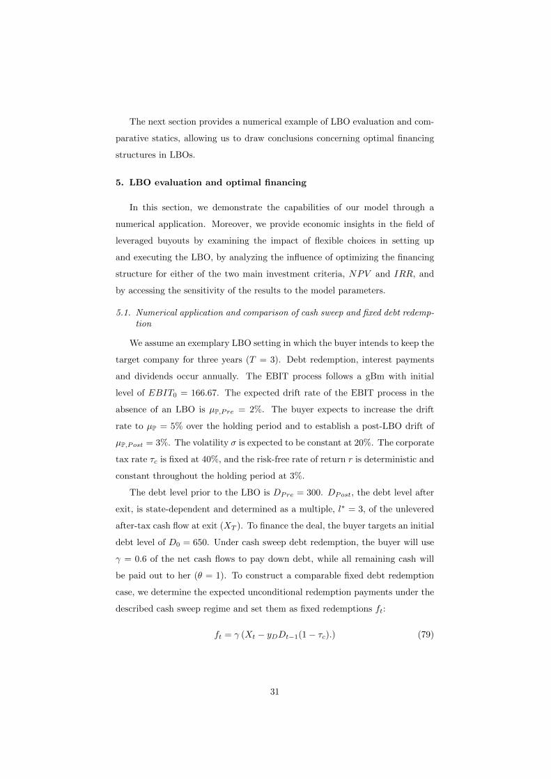
184.45 = NPV fixed, IRRsweep = 15.83 > 13.19 = IRRfixed).

The results may create the impression that cash sweep debt redemption is

dominating fixed debt redemption. However, analyzing the dynamics of this

relationship reveals contrary insights.

22

,ℚ ,ℚ

Def

ault

boun

dary

in t

=1

()

Cash sweep ratio (γ)





Prom

ised

yie

ld (

)

Inte

rnal

rat

e of

ret

urn

()

Net

pre

sent

val

ue (

)

Cum

. pr

obab

ility

of

defa

ult

(,ℚ

)

Figure 3: Cash sweep redemption versus fixed redemption for different cash sweep ratios γand the basic set of parameters as in Table 3. This figure depicts the promised yield (yD),the cumulative risk-neutral probability (cdT,Q), the internal rate of return (IRR), the netpresent value (NPV ) and the default boundary of period 1 over the interval of γ ∈ [0, 0.7] forcash sweep redemption (black, solid line) and fixed redemption (blue, dotted line). The fixeddebt redemption payments are matched to the cash sweep redemption ratio γ as defined byEquation (79).

34

Figure 3 shows that for moderate levels of the cash sweep ratio (0 < γ ≤

0.59), translating to moderate fixed cash obligations, the promised yield yD is

lower under fixed debt redemption. This triggers a lower cumulative default

probability (cdT,Q), a higher IRR and an increased NPV over a γ interval

of 0 < γ ≤ 0.52. The bottom graph in Figure 3 provides the first part of

the explanation: For moderate γ values, both redemption policies face a default

boundary determined by the covenant condition rather than the cash obligation.

The fixed cash obligation increases substantially with increasing values of γ,

resulting in a switch in the default trigger at γ = 0.56. The rationale from a

debtholders’ perspective is straightforward: As long as the default boundary is

identical for both types of redemption, fixed redemption delivers higher payoffs

in adverse (going concern) states. In other words, the flexibility of the cash

sweep redemption requires a premium. As soon as the default boundary for

the fixed case exceeds the one of the cash sweep case, the higher probability of

default for the fixed case makes the cash sweep case more favorable, generating

a trade-off that quickly results in an increasing promised yield. The second part

of the explanation is less trivial. While the two curves for default boundary

and promised yield cross at γ = 0.59 and γ = 0.56, respectively, the curves

for probability of default, IRR and NPV intersect earlier at γ = 0.52. This is

caused by the path-dependency of the default boundary under cash sweep debt

redemption. Note that the graph only depicts the first period’s default boundary

because the subsequent ones are path-dependent and, thus, not comparable on

an aggregated level. A high cash flow in the first period reduces the covenant

trigger of the subsequent periods, resulting in a lower probability of default

followed by higher expected payoffs. This effect of the reduction of the default

boundary causes the IRR and NPV shift as illustrated.

Based on this analysis, we can clearly state that the flexibility of cash sweep

debt redemption adds significant value for investors in LBOs and reduces the

risk of default for target companies as long as the corresponding fixed cash

obligations in any period exceed the covenant restriction. However, if fixed cash

obligations are moderate, i.e., remain well below the covenant condition, the

pricing of debt will be lower because cash flows to the debtholders are fixed

reducing the credit risk. In such cases, fixed debt redemption is more beneficial

35

for the equityholders because the lower promised yield translates into higher

payoffs, lower default probability (due to higher payoffs) and, thus, to increases

in NPV and IRR.

To conclude, our results provide an economic rationale for the widespread

phenomenon of mixed (cash sweep and fixed) financing structures in LBOs.

Fixed debt is available at lower prices as long as the cash obligations are not

critical to the firm’s going concern. Buyers in LBOs exploit this fact by filling

senior tranches with fixed debt and adding junior cash sweep debt to exploit

the benefits of debt without material increases in the probability of default.

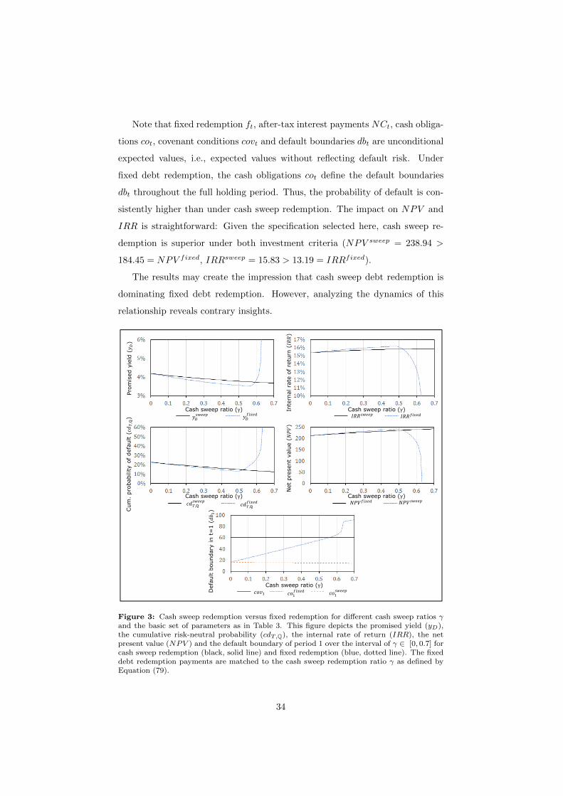
5.2. Optimal financing for NPV and IRR maximization

Investors in LBOs typically apply the IRR, both for investment and financing

decisions and for performance measurement (see, e.g., Gompers et al., 2015),

although academics have postulated for more than 50 years that there are serious

difficulties and pitfalls associated with this decision criterion (see, e.g., Lorie

and Savage, 1949, and Hirshleifer, 1958). Brealey, Myers and Allen provided

the classic critique in the first edition of “Principles of Corporate Finance” and

continue to do so (Brealey et al., 2013). We skip the discussion of these well-

known pitfalls, Footnote 2 of the introduction section contains a brief summary.

Our focus is on the impact of the investment criterion choice in a dynamic

setting with stochastic cash flows and explicit risk of default.

For the analysis, we consider the cash sweep policy introduced in the previ-

ous section but vary the initial debt level to identify the optimal leverage that

maximizes NPV or IRR. Figure 4 summarizes the results graphically.

Choosing the initial debt level based on a maximized IRR implies D0 = 650

and results in IRR = 15.83%. The corresponding NPV of this structure is

238.94. In turn, when we optimize the initial debt level for maximizing the

NPV criterion, we arrive at D0 = 460 with NPV = 267.55. Thus, optimizing

the initial debt level by the IRR criterion led to an NPV reduction of 10.69%.

Moreover, the IRR criterion fostered risk taking: The cumulative default prob-

ability over the holding period is cdT,Q = 13.41%, while for the NPV -optimal

debt level (D0 = 460) cdT,Q only amounts to 0.99%.

The results provide insights into the IRR vs. NPV discussion beyond the

classical arguments based on static frameworks. Our model allows for a precise

36

comparison concerning value creation and risk taking. The numerical results

indicate that the IRR criterion encourages investors to choose higher leverage,

which in turn increases default probability and reduces NPV creation.

A formal mathematical proof of this finding is beyond the scope of this paper

and remains for further research. However, we present the basic intuition: The

IRR approach discounts future expected cash flows stronger than the NPV

method, because it uses the risk-neutral IRR as a discount rate instead of the

risk-free rate r. Therefore, low initial equity investments, which are driven by

high initial debt levels, receive a higher weight. In contrast, reductions of the

expected cash flows over the holding period (particularly towards the end of

the holding period), driven by an increased risk of default, have a lower impact

because of the higher discount rate. Thus, the optimal trade-off between benefits

and costs of debt are different for the two investment criteria.

The sensitivity analyses in the next section add further robustness to our

findings. Note that the results under fixed debt redemption are equivalent. We

provide them in Appendix D.1.

37

Promised

yield (

)Internal rate of return (

)Net present value (

)Cum. probability of default (

,ℚ)

,ℚ=0.99%

Optimal D0 for IRR = 650

,ℚ=13.41%

NPV=267.55

NPV=238.94

IRR=14.00%IRR=15.83%

Optimal D0 for NPV = 460

yD=3.10%

yD=3.72%

Debt level ( )

Debt level ( )

Debt level ( )

Debt level ( )

Base Case Cash Sweep ‐ new

Figure 4: Optimal initial debt level for maximizing NPV or IRR. This figure depicts thepromised yield yD (first graph), the cumulative risk-neutral probability over the full holdingperiod cdT,Q (second graph), the IRR (third graph), and the NPV (fourth graph), each asa function of the initial debt level over the interval of D0 ∈ [350, 850]. We use the basic setof parameters reported in Table 3 and the financing parameters for cash sweep redemptionas illustrated in Table 4. The optimal initial debt level D0 for maximizing the NPV (blue,dashed line) or the IRR (red, small dashed line) are shown in all four graphs.

38

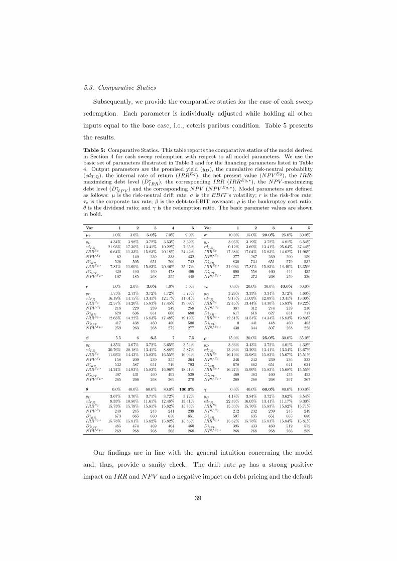
5.3. Comparative Statics

Subsequently, we provide the comparative statics for the case of cash sweep

redemption. Each parameter is individually adjusted while holding all other

inputs equal to the base case, i.e., ceteris paribus condition. Table 5 presents

the results.

Table 5: Comparative Statics. This table reports the comparative statics of the model derivedin Section 4 for cash sweep redemption with respect to all model parameters. We use thebasic set of parameters illustrated in Table 3 and for the financing parameters listed in Table4. Output parameters are the promised yield (yD), the cumulative risk-neutral probability(cdT,Q), the internal rate of return (IRREq), the net present value (NPV Eq), the IRR-maximizing debt level (D∗IRR), the corresponding IRR (IRREq,∗), the NPV -maximizing

debt level (D∗NPV ) and the corresponding NPV (NPV Eq,∗). Model parameters are definedas follows: µ is the risk-neutral drift rate; σ is the EBIT ’s volatility; r is the risk-free rate;τc is the corporate tax rate; β is the debt-to-EBIT covenant; ρ is the bankruptcy cost ratio;θ is the dividend ratio; and γ is the redemption ratio. The basic parameter values are shownin bold.

Var 1 2 3 4 5 Var 1 2 3 4 5

µP 1.0% 3.0% 5.0% 7.0% 9.0% σ 10.0% 15.0% 20.0% 25.0% 30.0%

yD 4.34% 3.98% 3.72% 3.53% 3.39% yD 3.05% 3.19% 3.72% 4.81% 6.54%cdT,Q 21.93% 17.30% 13.41% 10.22% 7.65% cdT,Q 0.12% 3.69% 13.41% 25.64% 37.44%IRREq 6.64% 11.33% 15.83% 20.18% 24.42% IRREq 17.38% 17.04% 15.83% 14.02% 11.96%NPV Eq 62 149 239 333 432 NPV Eq 277 267 239 200 159D∗IRR 526 595 651 700 742 D∗IRR 830 734 651 579 532IRREq,∗ 7.81% 11.60% 15.83% 20.46% 25.47% IRREq,∗ 21.09% 17.81% 15.83% 14.49% 13.35%D∗NPV 420 440 460 478 499 D∗NPV 690 558 460 444 435NPV Eq,∗ 107 185 268 355 448 NPV Eq,∗ 277 272 268 259 236

r 1.0% 2.0% 3.0% 4.0% 5.0% τc 0.0% 20.0% 30.0% 40.0% 50.0%


β 5.5 6 6.5 7 7.5 ρ 15.0% 20.0% 25.0% 30.0% 35.0%


θ 0.0% 40.0% 60.0% 80.0% 100.0% γ 0.0% 40.0% 60.0% 80.0% 100.0%


Our findings are in line with the general intuition concerning the model

and, thus, provide a sanity check. The drift rate µP has a strong positive

impact on IRR and NPV and a negative impact on debt pricing and the default

39

probability. A higher drift rate, i.e., increased EBIT performance over the

holding period, allows for higher optimal debt capacities irrespective of the

applied decision criterion.

For the cash flow’s volatility σ, the effects are reversed: Greater uncertainty

requires a higher promised yield for the debtholders, raises the risk of default

and reduces the results of both decision criteria. Consistently, the optimal debt

levels for maximizing IRR and NPV decrease.

The impact of the risk-free rate r is twofold. On the one hand, an increased

risk-free rate means higher discount factors, leading to a higher promised yield

yD and a lower NPV . Subsequently, an increase in yD yields higher interest pay-

ments and, thus, forces down the IRR and entails a higher default probability.

On the other hand, ceteris paribus, a rise in r yields a higher risk-neutral drift

due to the relationship µ = µP − (rA − r). As analyzed above, increasing drift

rates have exactly the opposite effects on IRR, NPV and default probability.

Because the second effect exceeds the first, overall, we find a positive relation-

ship between r and the decision criteria, as well as a negative relationship with

respect to the cumulative default probability.

The corporate tax rate τc has a positive impact on the promised yield yD

and cumulative default probability cdT,Q, i.e., a higher τc drives increases in

yD and cdT,Q because less cash is available to serve the debtholders during

the holding period and the liquidation value in event of default is also reduced.

Hence, a negative relationship with respect to the NPV is a logical consequence.

For the IRR, we find the opposite effect, which at first glance may appear

surprising. However, the nature of the IRR determination perfectly explains

the phenomenon. An increased corporate tax rate reduces future cash flows but

also reduces the initial investment, which has a much higher weight under the

IRR criterion in contrast to the NPV criterion. This property of the IRR also

causes the optimal initial debt level for maximizing the IRR (D∗IRR) to move

contrary to D∗NPV .

For the covenant ratio β, we find the same straightforward relationships as

for the drift rate µP. A less tight covenant, i.e., β moves upwards, leads to

decreasing default probabilities cdT,Q and a lower promised yield yD and has a

positive impact on the investment criteria IRR and NPV . Consistently, the

40

optimal debt levels are higher.

A rise in the bankruptcy cost ratio ρ triggers the exact opposite results,

which are clearly due to the reduced liquidation value in the event of default.

The impact of the dividend ratio θ on the model parameters is of very small

magnitude relative to the other parameters. Moreover, the direction of the ef-

fects is as expected: Lower dividends foster excess cash holdings, creating a

cushion against default. Thus, the dividend ratio and probability of default

cdT,Q have a positive relationship, which triggers a negative impact on the

promised yield yD and the NPV . We find the opposite regarding the IRR,

again caused by the fact that earlier cash flows (dividends received over the

holding period) are valued higher than later cash flows (excess cash paid out at

exit).

The effects generated by a change in the cash sweep ratio γ depend on a

trade-off. A high γ reduces the debt burden more quickly, relaxes the covenant

condition, and subsequently generates lower costs of debt yD, lower default

probabilities cdT,Q and thus increased expected future payoffs. By contrast,

a more rapid reduction of debt gives away tax savings and shifts cash flows

from the beginning of the holding period towards the end (relevant for the IRR

criterion). Which of the two effects dominates depends on the initial debt level.

Figure 5 presents in detail the trade-off we described.

Thus, we find different effects concerning NPV and IRR for our base case

debt level of D0 = 650. The NPV -curves for the different γ-values have already

crossed such that a higher γ generates an increased NPV . The IRR-curves,

however, have not fully switched their positions. The first time the IRR is

consistently increasing with γ is at D0 = 684. At our base case debt level,

γ = 0.6 generates the highest IRR.

Overall, the comparative statics demonstrate the robustness of the model.

All model outputs created by changes in the input parameters conform to eco-

nomic intuition. A complete comparative statics report regarding fixed debt

redemption has also been drafted and is presented in Appendix D.2.

41

22

Prom

ised

yie

ld (

)

Inte

rnal

rat

e of

ret

urn

()

Net

pre

sent

val

ue (

)

Cum

. pr

obab

ility

of

defa

ult

(,ℚ

)

γ 0.0γ 0.6

γ 0.2γ 0.8

γ 0.4γ 1.0

Debt level ( )

γ 0.0γ 0.6

γ 0.2γ 0.8

γ 0.4γ 1.0

Debt level ( )

γ 0.0γ 0.6

γ 0.2γ 0.8

γ 0.4γ 1.0

Debt level ( )

γ 0.0γ 0.6

γ 0.2γ 0.8

γ 0.4γ 1.0

Debt level ( )

Figure 5: Detailed comparative analysis for cash sweep ratio γ. The figure illustrates thepromised yield yD (upper-left graph), the cumulative risk-neutral probability over the fullholding period cdT,Q (lower-left graph), the IRR (up-right graph), and the NPV (lower-rightgraph), each as a function of the initial debt level over the interval of D0 ∈ [350, 875] forγ ∈ [0, 1]. All other input parameters are as defined in the basic set reported in Table 3.

6. Conclusion

Target firms in an LBO setting follow a different capital structure and re-

demption policy than their peers. Initially financed by a large portion of debt,

leverage is reduced stepwise over the holding period. In this article, we im-

plement these dynamics in a model based on a boundary-crossing approach

that allows for a non-differentiable functional form of the barrier to evaluate its

financial effects.

Methodologically, our contribution can be summarized as follows. The

method employed in this paper allows to capture both types of debt redemp-

tion found in LBO settings: the fixed, predetermined one and the dynamic,

path-dependent one known as “cash sweep”. Based upon these stepwise re-

demptions, we implement a discontinuous, non-differentiable lower boundary for

mapping the default trigger. We allow for flexibility, as these boundaries can

be either derived from cash obligations (redemption plus interest payments) or

covenants (e.g., debt-to-EBIT ratio). By extending the approach of Wang and

Potzelberger (1997), wea are able to determine default probabilities using nested

integrals that can be solved numerically. This enables us to provide explicit-

42

form solutions for the evaluation of LBO investments using the NPV and IRR

criteria. Additionally, the model captures the pricing of debt endogenously,

which allows to also evaluate LBO structures from a debtholder perspective.

Our model makes some significant contributions to economic theory. We

show that firms using a cash sweep redemption can create significant additional

value for investors by reducing the risk of default due to the path-dependency

of the redemption payments. However, we also find that for moderate fixed

cash obligations, i.e., cash obligations are not critical as a default trigger, the

promised yield of debt decreases as cash flows to debtholders are less exposed

to credit risk. Equityholders are better off in such setups irrespective of the

decision criterion employed because interest payments are reduced. Thus, our

model explains why buyers in LBOs apply mixed financing structures, senior

moderate levels of fixed debt and junior cash sweep debt. Furthermore, when

stepwise optimizing the capital structure for either NPV or IRR, we find novel

insights beyond the classic critics of the IRR. The entry debt level maximizing

the IRR is strictly higher than the debt level implied by maximizing the NPV .

In turn, this is reflected by a higher default probability for the IRR-maximizing

case. Comparing the two decision criteria with respect to value creation, we

find that the IRR criterion causes a significant NPV reduction.

Nonetheless, some limitations of our approach have to be addressed. We do

not address the positive and negative wealth effects of corporate debt beyond tax

savings and default. Debt provides several advantages for an LBO investor by re-

ducing overinvestment and agency problems and, thus, the cost associated with

them (Jensen and Meckling, 1976). On the opposite side, debt overhang and

underinvestment are particular debt-related disadvantages not covered by our

model. Additionally, as our model optimizes IRR and NPV at the firm level,

we do not differentiate between general and limited partners usually engaged in

PE investments. Therefore, including their typical compensation schemes might

be a potential area of further research.

Finally, because the nested integral approach allows for several conditions,

the model is easily extendable, e.g., to rules limiting the tax deductibility of

interest payments.

43

A. Appendix: Stochastic calculus for Brownian motion with drift andconstant lower boundary

A.1. Density function of Brownian motion with drift and its minimum

In this section, we derive the joint density function of a Brownian motion

with drift Wt and its minimum Mt.

First, we begin with a Brownian motion without drift Wt and adjust it in a

way that a Brownian motion with drift Wt is generated:

Wt = αt+Wt. (80)

Next, we define the minimum Mt of such a process under the prerequisites

Mt ≤ 0 and Wt ≥ Mt:

Mt = min0≤t≤T

Wt. (81)

According to the Girsanov Theorem, we define a new probability measure

Q under which Wt has zero drift:

Zt = e−αWt− 12α

2·t = e−αWt+12α

2t (82)

Q(A) =

∫A

ZT dQ (83)

For a process without drift, we know the joint density function with its

minimum from the Reflection Principle (for detailed derivation, see, for example,

Shreve, 2004):

fMt,Wt(m,w) =

2(w − 2m)

t√

2πte−(2m−w)2

2t (84)

Finally, we can derive the density of Mt and Wt under Q, the risk-neutral

probability measure:

44

QMt ≥ m, Wt ≥ w = EQIMt≥m,Wt≥w

= EQ1

ZtIMt≥m,Wt≥w

= EQeαWt−12α2tIMt≥m,Wt≥w

=

∞∫m

∞∫w

eαY−12α2T fMt,Wt(x, y)dxdy

δ2QMt ≥ m, Wt ≥ wδmδw

= eαw−12α2tfMt,Wt(m,w)

=2(w − 2m)

t√2πt

eαw−12α2t− (2m−w)2

2t . (85)

A.2. Default and going concern probability of Brownian motion with drift versusa constant default barrier

Based on the density function of Mt and Wt under Q (Equation (85)), we

derive the default and going concern probabilities of a Brownian motion with

drift versus a constant default barrier. We begin with the going concern proba-

bility. Thus, the relevant set of values m and w is (m,w);w ≥ m,m ≤ 0. We

integrate the density function over this region to determine:

QMT ≥ m =0∫

m

w∫m

2(v − 2m)

T√2πT

eαw−12α2T− (2v−w)2

2T dvdw

+

∞∫0

0∫m

2(v − 2m)

T√2πT

eαw−12α2T− (2v−w)2

2T dvdw (86)

=

0∫m

[1√2πT

eαv−α2T

2− (2v−w)2

2T

]vm

dw

+

∞∫0

[1√2πT

eαv−α2T

2− (2v−w)2

2T

]m0

dw (87)

=

0∫m

1√2πT

eαw−α2T

2−w

2

2T dw −0∫

m

1√2πT

eαw−α2T

2− (2m−w)2

2T dw

+

∞∫0

1√2πT

eαw−α2T

2−w

2

2T dw −∞∫0

1√2πT

eαw−α2T

2− (2m−w)2

2T dw. (88)

Next, we follow the approach of Shreve (2004) and complete the squares:

45

αw − α2T

2− (2m− w)2

2T= − 1

2T(w − 2m− αT )2 + 2αm, (89)

αw − α2T

2− w2

2T= − 1

2T(w − αT )2, (90)

Thus, we can transform Equation (88) to:

QMT ≥ m =1√2πT

∞∫m

e−1

2T(w−αT )2dw − e2αm

∞∫m

e−1

2T(w−2m−αT )2dw

(91)

By substituting y1 = w−αT√T

in the first integral and y2 = w−2m−αT√T

in the

second integral, we obtain:

QMT ≥ m =1√2πT

∞∫

m−αT√T

e−12y

21dy1 − e2αm

∞∫−m−αT√

T

e−12y

22dy2

= N

(−m− αT√

T

)− e2αmN

(m+ αT√

T

). (92)

Equation (92) represents the going concern probability. The default proba-

bility is simply the probability of the counter event, hence we arrive at:

QMT < m = 1−[N

(−m− αT√

T

)− e2αmN

(m+ αT√

T

)]= N

(m− αT√

T

)+ e2αmN

(m+ αT√

T

). (93)

Equation (93) is equal to Equation (51) from Section 3.

B. Appendix: Transformation of value conditions

In Section 2 of this paper, we define conditions concerning the payoffs in our

model. During the derivation of our explicit integral-form solutions in Section

4, we present the first three of these conditions rearranged for the standard nor-

mally distributed random variable xt, thereby allowing us to restrict the limits

of the integrals (Equations (67) to (69)). Subsequently, we show the transfor-

mation in detail and examine the three deterministic conditions for liquidation

value of equity and debt.

46

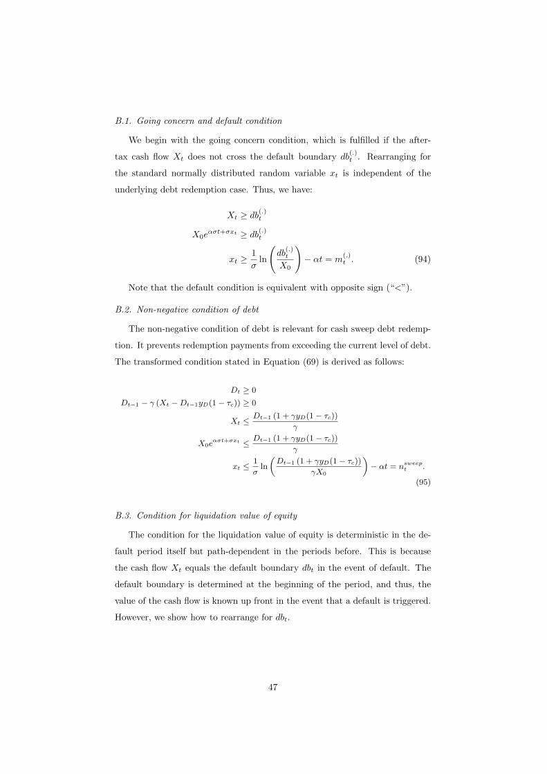
B.1. Going concern and default condition

We begin with the going concern condition, which is fulfilled if the after-

tax cash flow Xt does not cross the default boundary db(.)t . Rearranging for

the standard normally distributed random variable xt is independent of the

underlying debt redemption case. Thus, we have:

Xt ≥ db(.)t

X0eασt+σxt ≥ db(.)t

xt ≥1

σln

(db

(.)t

X0

)− αt = m

(.)t . (94)

Note that the default condition is equivalent with opposite sign (“<”).

B.2. Non-negative condition of debt

The non-negative condition of debt is relevant for cash sweep debt redemp-

tion. It prevents redemption payments from exceeding the current level of debt.

The transformed condition stated in Equation (69) is derived as follows:

Dt ≥ 0

Dt−1 − γ (Xt −Dt−1yD(1− τc)) ≥ 0

Xt ≤Dt−1 (1 + γyD(1− τc))

γ

X0eασt+σxt ≤ Dt−1 (1 + γyD(1− τc))

γ

xt ≤1

σln

(Dt−1 (1 + γyD(1− τc))

γX0

)− αt = nsweept .

(95)

B.3. Condition for liquidation value of equity

The condition for the liquidation value of equity is deterministic in the de-

fault period itself but path-dependent in the periods before. This is because

the cash flow Xt equals the default boundary dbt in the event of default. The

default boundary is determined at the beginning of the period, and thus, the

value of the cash flow is known up front in the event that a default is triggered.

However, we show how to rearrange for dbt.

47

Xt +XCt + (1− ρ)V Ut −Dt−1 −Dt−1yD(1− τc) > 0

Xt

(1 + (1− ρ)

eµ

er − eµ

)> Dt−1 +Dt−1yD(1− τc)−XCt

Substituting Xt = db(.)t yields:

db(.)t >

Dt−1 +Dt−1yD(1− τc)−XCt1 + (1− ρ) eµ

er−eµ. (96)

B.4. Condition for liquidation value of debt

The condition for the liquidation value of debt is also deterministic in the

default period itself but path-dependent in the periods before. This is because

the cash flow Xt equals the default boundary dbt in the event of default. The

default boundary is determined at the beginning of the period, and thus, the

value of the cash flow is known up front in the event that a default is triggered.

However, we show how to rearrange condition 1 for dbt.

(1− ρ)V Ut > Dt−1yD +Dt−1

Xteµ

er − eµ>Dt−1(1 + yD)

1− ρ

Substituting Xt = db(.)t yields:

db(.)t >

Dt−1(1 + yD)

(1− ρ) eµ

er−eµ. (97)

Note that condition 2 for the liquidation value of debt is equivalent with

opposite sign (“≤”).

C. Appendix: Explicit analytic-form solution of value componentsfor θ = 1 and γ = 0

While our approach works for any LBO financing structure, delivering solu-

tion formulae in explicit integral form, there exists a special case that collapses

to an explicit analytic form. This case requires three special assumptions: (1)

no excess cash at the beginning of the holding period (XC0 = 0), (2) no debt

redemption over the holding period (γ = 0), and (3) full payout of free equity

cash flows over the holding period (θ = 1).

48

Under these prerequisites, the default boundary is constant over the course

of the LBO, and there exists no difference between redemption cases (db =

dbsweept = dbfixedt ). The default barrier db is defined as the maximum of covenant

and cash obligation, which can be obtained deterministically from the outset:

db = max

(D0yD(1− τc),

D0

β(1− τc)

). (98)

The formula for the cumulative default probability is equivalent to Equation

(51):

cdt,Q = QMt < m

= N

(m− αt√

t

)+ e2αmN

(m+ αt√

t

), (99)

with

α =1

σ

(µ− σ2

2

), (100)

m =1

σln

(db

X0

). (101)

Based on Equation (99), we obtain the incremental default probability of a

single period as:

pdt,Q = cdt,Q − cdt−1,Q. (102)

The present values for the equity cash flows over the course of the holding

period are equivalent to barrier down-and-out call options with rebate values.

The formula for such an option translated to our problem is as follows:

PVt =C(Xt, db)−(db

X0

)2ασ

C(db2

Xt, db)

+ (db− co)e−rt(N(d2(Xt, db))−

(db

X0

)2ασ

N(d2(db2

Xt, db))

)

+ pdt(1− ρ)dbeµ

er − eµ, (103)

49

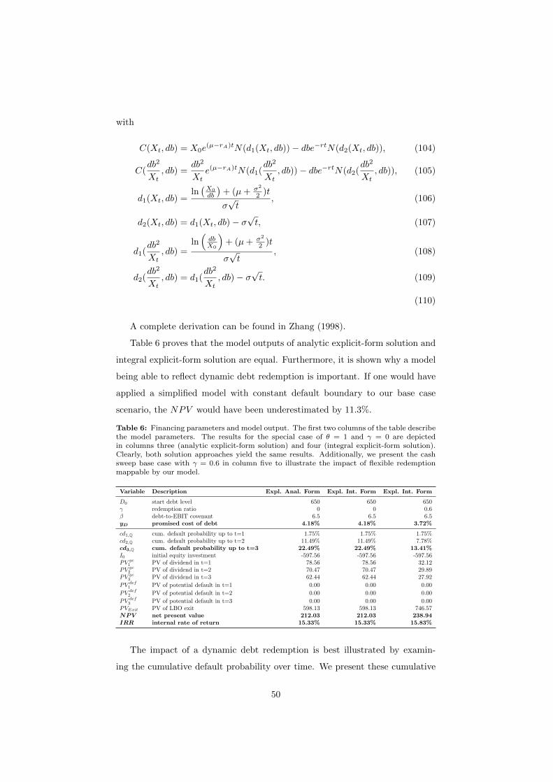
with

C(Xt, db) = X0e(µ−rA)tN(d1(Xt, db))− dbe−rtN(d2(Xt, db)), (104)

C(db2

Xt, db) =

db2

Xte(µ−rA)tN(d1(

db2

Xt, db))− dbe−rtN(d2(

db2

Xt, db)), (105)

d1(Xt, db) =ln(X0

db

)+ (µ+ σ2

2 )t

σ√t

, (106)

d2(Xt, db) = d1(Xt, db)− σ√t, (107)

d1(db2

Xt, db) =

ln(dbX0

)+ (µ+ σ2

2 )t

σ√t

, (108)

d2(db2

Xt, db) = d1(

db2

Xt, db)− σ

√t. (109)

(110)

A complete derivation can be found in Zhang (1998).

Table 6 proves that the model outputs of analytic explicit-form solution and

integral explicit-form solution are equal. Furthermore, it is shown why a model

being able to reflect dynamic debt redemption is important. If one would have

applied a simplified model with constant default boundary to our base case

scenario, the NPV would have been underestimated by 11.3%.

Table 6: Financing parameters and model output. The first two columns of the table describethe model parameters. The results for the special case of θ = 1 and γ = 0 are depictedin columns three (analytic explicit-form solution) and four (integral explicit-form solution).Clearly, both solution approaches yield the same results. Additionally, we present the cashsweep base case with γ = 0.6 in column five to illustrate the impact of flexible redemptionmappable by our model.

Variable Description Expl. Anal. Form Expl. Int. Form Expl. Int. Form

D0 start debt level 650 650 650γ redemption ratio 0 0 0.6β debt-to-EBIT covenant 6.5 6.5 6.5yD promised cost of debt 4.18% 4.18% 3.72%

cd1,Q cum. default probability up to t=1 1.75% 1.75% 1.75%cd2,Q cum. default probability up to t=2 11.49% 11.49% 7.78%cd3,Q cum. default probability up to t=3 22.49% 22.49% 13.41%I0 initial equity investment -597.56 -597.56 -597.56PV gc1 PV of dividend in t=1 78.56 78.56 32.12PV gc2 PV of dividend in t=2 70.47 70.47 29.89PV gc3 PV of dividend in t=3 62.44 62.44 27.92

PV def1 PV of potential default in t=1 0.00 0.00 0.00

PV def2 PV of potential default in t=2 0.00 0.00 0.00

PV def3 PV of potential default in t=3 0.00 0.00 0.00PVExit PV of LBO exit 598.13 598.13 746.57NPV net present value 212.03 212.03 238.94IRR internal rate of return 15.33% 15.33% 15.83%

The impact of a dynamic debt redemption is best illustrated by examin-

ing the cumulative default probability over time. We present these cumulative

50

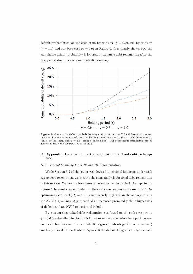
default probabilities for the case of no redemption (γ = 0.0), full redemption

(γ = 1.0) and our base case (γ = 0.6) in Figure 6. It is clearly shown how the

cumulative default probability is lowered by dynamic debt redemption after the

first period due to a decreased default boundary.

25

γ 0.0 γ 0.6 γ 1.0Holdingperiod

Cum.probabilityofdefault

,ℚ

Figure 6: Cumulative default probability (cdt until point in time T for different cash sweepratios γ. The figure depicts cdt over the holding period for γ = 0.0 (black, solid line), γ = 0.6(blue, dotted line), and γ = 1.0 (orange, dashed line). All other input parameters are asdefined in the basic set reported in Table 3.

D. Appendix: Detailed numerical application for fixed debt redemp-tion

D.1. Optimal financing for NPV and IRR maximization

While Section 5.2 of the paper was devoted to optimal financing under cash

sweep debt redemption, we execute the same analysis for fixed debt redemption

in this section. We use the base case scenario specified in Table 3. As depicted in

Figure 7 the results are equivalent to the cash sweep redemption case: The IRR-

optimizing debt level (D0 = 715) is significantly higher than the one optimizing

the NPV (D0 = 254). Again, we find an increased promised yield, a higher risk

of default and an NPV reduction of 9.60%.

By constructing a fixed debt redemption case based on the cash sweep ratio

γ = 0.6 (as described in Section 5.1), we examine a scenario where path depen-

dent switches between the two default triggers (cash obligation vs. covenant)

are likely. For debt levels above D0 = 713 the default trigger is set by the cash

51

obligation right from the beginning of the holding period. The observed double-

peak in the NPV -curve at D0 = 254 (our global maximum) and at D0 = 680

is a direct consequence of these path-dependent switches.

Please note that if one chooses a lower cash sweep ratio (e.g.,γ = 0.5),

the graphs look similar to the ones under cash sweep debt redemption (see e.g.

Figure 4) as the default trigger switches to the debt-to-EBIT covenant condition

for all debt levels.

D.2. Comparative statics

We provide a sensitivity analysis for fixed debt redemption equivalent to the

comparative statics regarding cash sweep debt redemption (Table 5. To ensure a

valid comparison between the redemption cases, we match the fixed redemption

payments again to the expected cash sweep redemption payments as described

in Equation (79). This matching triggers a specific feature we outline at the

beginning: Whenever a change in parameters lead to changes in the expected

EBIT , we face an adjustment of the fixed redemption payments.

Thus, some effects depicted in Table 7 are slightly different than in Sec-

tion 5.3. Exemplarily, an increase in µP causes higher expected EBIT figures

and, consequently, higher fixed cash obligations. The cumulative risk of default

(cdT,Q) increases because the effect of higher cash obligations exceed the effect

of the improved EBIT process. Beyond this peculiarity, the results generated

by changes in µP are consistent with the cash sweep redemption case.

52

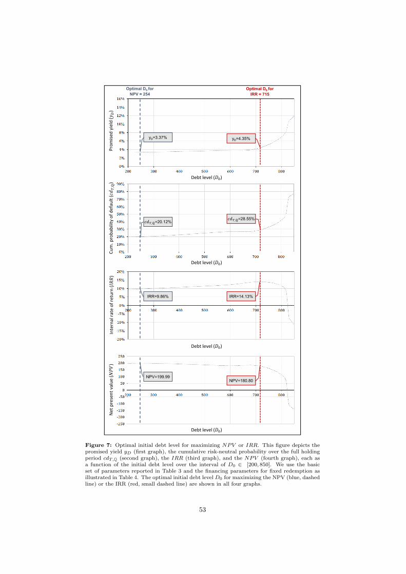
Promised

yield (

)Internal rate of return (

)Net present value (

)Cum. probability of default (

,ℚ)

,ℚ=20.12%

Optimal D0 for IRR = 715

,ℚ=28.55%

NPV=199.99NPV=180.80

IRR=9.86% IRR=14.13%

Optimal D0 for NPV = 254

yD=3.37% yD=4.35%

Debt level ( )

Debt level ( )

Debt level ( )

Debt level ( )

Base Case Fixed – new (0.6)

Figure 7: Optimal initial debt level for maximizing NPV or IRR. This figure depicts thepromised yield yD (first graph), the cumulative risk-neutral probability over the full holdingperiod cdT,Q (second graph), the IRR (third graph), and the NPV (fourth graph), each asa function of the initial debt level over the interval of D0 ∈ [200, 850]. We use the basicset of parameters reported in Table 3 and the financing parameters for fixed redemption asillustrated in Table 4. The optimal initial debt level D0 for maximizing the NPV (blue, dashedline) or the IRR (red, small dashed line) are shown in all four graphs.

53

Table 7: Comparative Statics for fixed debt redemption. This table reports the comparativestatics of the model derived in Section 4 for fixed debt redemption with respect to all modelparameters. We use the basic set of parameters illustrated in Table 3 and for the financingparameters those listed in Table 4. Output parameters are the promised yield (yD), the cu-mulative risk-neutral probability (cdT,Q), the internal rate of return (IRREq), the net presentvalue (NPV Eq), the IRR-maximizing debt level (D∗IRR), the corresponding IRR (IRREq,∗),

the NPV -maximizing debt level (D∗NPV ) and the corresponding NPV (NPV Eq,∗). Modelparameters are defined as follows: µ is the risk-neutral drift rate; σ is the EBIT ’s volatil-ity; r is the risk-free rate; τc is the corporate tax rate; β is the debt-to-EBIT covenant; ρ isthe bankruptcy cost ratio; θ is the dividend ratio; and γ is the redemption ratio. The basicparameter values are shown in bold.

Var 1 2 3 4 5 Var 1 2 3 4 5

µP 1.0% 3.0% 5.0% 7.0% 9.0% σ 10.0% 15.0% 20.0% 25.0% 30.0%

yD 4.04% 3.77% 3.81% 3.92% 4.04% yD 3.05% 3.14% 3.81% 9.13% 10.04%cdT,Q 25.59% 25.26% 26.78% 28.45% 30.11% cdT,Q 1.24% 10.64% 26.78% 72.81% 77.95%IRREq 5.89% 9.75% 13.19% 16.54% 19.81% IRREq 17.22% 15.98% 13.19% -4.12% -6.04%NPV Eq 48 118 184 252 322 NPV Eq 273 244 184 -101 -124D∗IRR 625 675 715 750 760 D∗IRR 835 775 715 303 120IRREq,∗ 5.94% 9.89% 14.13% 18.22% 22.37% IRREq,∗ 21.46% 17.97% 14.13% 8.09% 6.61%D∗NPV 245 249 254 259 263 D∗NPV 725 675 254 121 0NPV Eq,∗ 55 125 200 278 359 NPV Eq,∗ 275 244 200 159 109

r 1.0% 2.0% 3.0% 4.0% 5.0% τc 0.0% 20.0% 30.0% 40.0% 50.0%

yD 1.49% 2.57% 3.81% 5.44% 9.98% yD 3.82% 3.90% 3.95% 3.81% 6.41%cdT,Q 19.40% 22.43% 26.78% 34.03% 66.99% cdT,Q 27.38% 28.34% 28.93% 26.78% 42.71%IRREq 12.09% 12.83% 13.19% 12.58% 0.00% IRREq 10.18% 10.84% 11.44% 13.19% 10.56%NPV Eq 207 200 184 150 -73 NPV Eq 282 225 197 184 91D∗IRR 675 700 715 700 450 D∗IRR 715 725 750 715 825IRREq,∗ 12.39% 13.43% 14.13% 13.29% 12.52% IRREq,∗ 10.38% 11.36% 12.34% 14.13% 21.48%D∗NPV 285 270 254 241 225 D∗NPV 0 318 298 254 213NPV Eq,∗ 206 203 200 197 193 NPV Eq,∗ 430 262 231 200 168

β 5.5 6 6.5 7 7.5 ρ 15.0% 20.0% 25.0% 30.0% 35.0%


θ 0.0% 40.0% 60.0% 80.0% 100.0% γ 0.0% 20.0% 40.0% 50.0% 60.0%


54

References

Achleitner, A.-K., Braun, R., Hinterramskogler, B., Tappeiner, F., 2012. Struc-

ture and determinants of financial covenants in leveraged buyouts. Review of

Finance 16, 647–684.

Arzac, E. R., 1996. Valuation of highly leveraged firms. Financial Analysts Jour-

nal 52 (4), 42–50.

Axelson, U., Jenkinson, T., Strı¿½mberg, P., Weisbach, M. S., 2013. Borrow

cheap, buy high? The determinants of leverage and pricing in buyouts. Jour-

nal of Finance 68 (6), 2223–2267.

Berg, A., Gottschalg, O., 2005. Understanding value creation in buyouts. Jour-

nal of Restructuring Finance 2, 9–37.

Braun, R., Engel, N., Hieber, P., Zagst, R., 2011. The risk appetite of private

equity sponsors. Journal of Empirical Finance 18 (5), 815–832.

Brealey, R., Myers, S., Allen, F., 2013. Principles of Corporate Finance, 11th

Edition. McGraw-Hill/Irwin, New York, NY.

Colla, P., Ippolito, F., Wagner, H. F., 2012. Leverage and pricing of debt in

LBOs. Journal of Corporate Finance 18 (1), 124–137.

Cooper, I. A., Nyborg, K. G., 2010. Consistent valuation of project finance and

LBO’s using the flows-to-equity method. Research Paper No. 10-51, Swiss

Finance Institute.

Couch, R., Dothan, M., Wu, W., 2012. Interest tax shields: A barrier options

approach. Review of Quantitative Finance and Accounting 39, 123–146.

Cox, J. C., Rubinstein, M., 1985. Options Markets. Vol. 340. Prentice-Hall,

Englewood Cliffs, NJ.

Flannery, M. J., Rangan, K. P., 2006. Partial adjustment toward target capital

structures. Journal of Financial Economics 79, 469–506.

Goldstein, R., Ju, N., Leland, H. E., 2001. An EBIT-based model of dynamic

capital structure. Journal of Business 74 (4), 483–512.

55

Gompers, P., Kaplan, S., Mukharlyamov, V., 2015. What do private equity

firms say they do? Working Paper No. 21133, NBER.

Hackbarth, D., Hennessy, C., Leland, H. E., 2007. Can the tradeoff theory

explain debt structure? Review of Financial Studies 20 (5), 1389–1428.

Hirshleifer, J., 1958. On the theory of optimal investment decision. Journal of

Political Economy 66 (4), 329–352.

Hotchkiss, E. S., Stromberg, P., Smith, D. C., 2014. Private equity

and the resolution of financial distress. Finance Working Paper No.

331/2012, ECGI, AFA 2012 Chicago Meetings Paper, available at SSRN:

http://ssrn.com/abstract=1787446.

Jensen, M., Meckling, W., 1976. Theory of the firm: Managerial behavior,

agency costs and ownership structure. Journal of Financial Economics 3 (4),

305–360.

Kaplan, S., Schoar, A., 2005. Private equity performance: Returns, persistence

and capital flows. Journal of Finance 60 (4), 1791–1823.

Kaplan, S., Stromberg, P., 2008. Leveraged buyouts and private equity. Journal

of Economic Perspectives 22 (4), 1–27.

Kim, J., Ramaswamy, K., Sundaresan, S., 1993. Does default risk in coupons

affect the valuation of corporate bonds?: A contingent claims model. Financial

Management, 117–131.

Kunitomo, N., Ikeda, M., 1992. Pricing options with curved boundaries. Math-

ematical Finance 2 (4), 275–298.

Leland, H. E., 1994. Corporate debt value, bond covenants, and optimal capital

structure. Journal of Finance 49 (4), 1213–1252.

Lo, C., Lee, H., Hui, C., 2003. A simple approach for pricing barrier options

with time-dependent parameters. Quantitative Finance 3, 98–107.

Lorie, J. H., Savage, L. J., 1949. Three problems in rationing capital. Journal

of Business 28 (4), 229–239.

56

Merton, R. C., 1973. Theory of rational option pricing. The Bell Journal of

Economics and Management Science 4 (1), 141–183.

Merton, R. C., May 1974. On the pricing of corporate debt: The risk structure

of interest rates. Journal of Finance 29 (2), 449–470.

Miles, J. A., Ezzell, J. R., 1980. The weighted average cost of capital, perfect

capital markets, and project life: A clarification. The Journal of Financial

and Quantitative Analysis 15 (3), 719–730.

Modigliani, F., Miller, M. H., 1963. Corporate income taxes and the cost of

capital: A correction. The American Economic Review 53 (3), 433–443.

Myers, S. C., 1974. Interactions of corporate financing and investment decisions-

implications for capital budgeting. Journal of Finance 29 (1), 1–25.

Rasmussen, P. N., 2009. Direct EU regulation for private equity and hedge funds

- The real economy comes first. In: Commission Conference on Private Equity

and Hedge Funds.

Roberts, G., Shortland, C., 1997. Pricing barrier options with time-dependent

coefficients. Mathematical Finance 7 (1), 83–93.

Rubinstein, M., Reiner, E., 1991. Unscrambling the binary code. Risk Magazine

4 (9), 75–83.

Shreve, S. E., 2004. Stochastic Calculus for Finance II - Continuous-Time Mod-

els. Springer-Verlag, New York, NY.

Strebulaev, I. A., Whited, T. M., 2011. Dynamic models and structural estfi-

nance in corporate finance. Foundations and Trends in Finance 6 (1-2), 1–163.

Stromberg, P., 2007. The new demography of private equity. Work-

ing paper, Swedish Institute for Financial Research, Stockholm

School of Economics, CEPR, and NBER, available at SIFR:

http://www.sifr.org/PDFs/stromberg(demography2008).pdf.

Tykvova, T., Borell, M., 2012. Do private equity owners increase risk of financial

distress and bankruptcy? Journal of Corporate Finance 18 (1), 138–150.

57

Wang, L., Potzelberger, K., 1997. Boundary crossing probability for brownian

motion and general boundaries. Journal of Applied Probability 34 (1), 54–65.

Wang, L., Potzelberger, K., 2007. Crossing probabilities for diffusion processes

with piecewise continuous boundaries. Methodology and Computing in Ap-

plied Probability 9 (1), 21–40.

Zhang, P. G., 1998. Exotic Options - A Guide to Second Generation Options,

2nd Edition. World Scientific Publishing Co. Pte. Ltd., Hackensack, NJ.

58

modeling dynamic redemption and default risk for lbo...

Documents