modeling energy and climate mitigation scenarios for brazil · modeling energy and climate...
TRANSCRIPT
Modeling Energy and Climate
Mitigation Scenarios for Brazil
Alexandre Szklo
Associate Professor
Energy Planning Program. Graduate School of Engineering
Universidade Federal do Rio de Janeiro
PPE/COPPE/UFRJ
Full version originally presente in EPE, November 9th 2016
1
Overview
The MSB300 IAM
The MSB 8000 IAM
Current research and the MS-
Global IAM (COFFEE)

Overview
1999: collaboration with UN-IAEA
Since then fifteen versions of the MSG-Brazil model
have been developed by our team
As of November 2016 => the first full version of COFFEE
(MSB-Global) is operational (land use and energy)
But all of this has only been made possible given the
large number of supporting studies done by our group:
almost 100 papers recently published (associated with
energy modelling + PhD thesis + Master Dissertation +
technical reports)
The Center for Energy and Environmental
Economics – CENERGIA (since 2003)
Our team at CENERGIA
Professors
Roberto Schaeffer
Alexandre Szklo
André F P Lucena
Researchers
Ten M.Sc. students, ten D.Sc. students and four Pos-Docs
(one third of the researchers are from abroad)
5
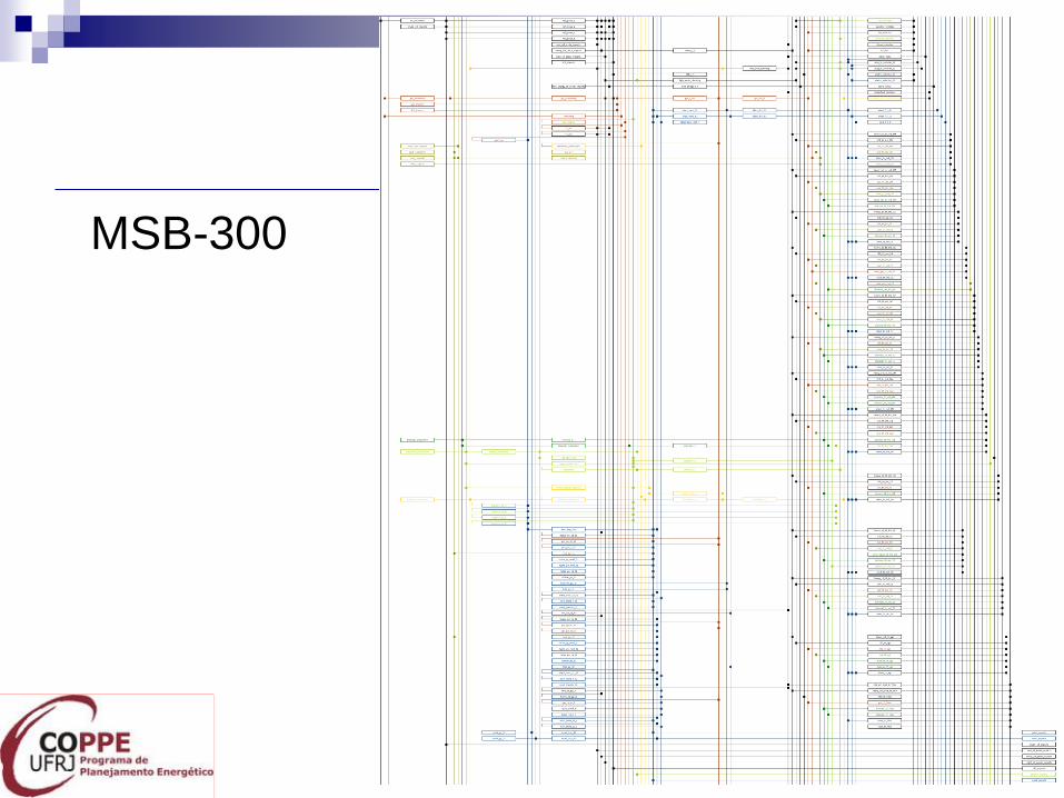
The MSB300
Our “compact model” already translated to GAMS and
translated to a full Brazilian Times Version (so-called
“TIMBRA”
It helped also to build TIMES_CONE SUR (gas-power
model – Southern Cone)
It is helping building TIMES-Peru
MESSAGE (MSG)
MSG is a mixed integer programming model
designed to formulate/evaluate alternative
strategies to supply energy subject to:
Investment limits
Availability and price of fuels
Environmental regulations
Market penetration rates for new technologies
Etc
8
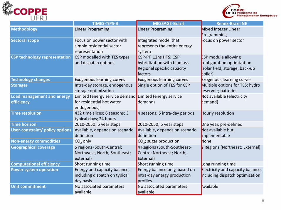
TIMES-TiPS-B MESSAGE-Brazil Remix-Brazil NEMethodology Linear Programing Linear Programing Mixed Integer Linear
ProgrammingSectoral scope Focus on power sector with
simple residential sector representation
Integrated model that represents the entire energy system
Focus on power sector
CSP technology representation CSP modelled with TES types and dispatch options
CSP-PT, 12hs HTS; CSP hybridization with biomass. Regional specific capacity factors
CSP module allowing configuration optimization (solar field, storage, back-up boiler)
Technology changes Exogenous learning curves Exogenous learning curves Exogenous learning curvesStorages Intra-day storage, endogenous
storage optimizationSingle option of TES for CSP Multiple options for TES; hydro
reservoir; batteriesLoad management and energy efficiency
Limited (energy service demand for residential hot water endogenous)
Limited (energy service demand)
Not available (electricity demand)
Time resolution 432 time slices; 6 seasons; 3 typical days; 24 hours
4 seasons; 5 intra-day periods Hourly resolution
Time horizon 2010-2050; 5 year steps 2010-2050; 5 year steps One year, pre-definedUser-constraint/ policy options Available, depends on scenario
definitionAvailable, depends on scenario definition
Not available but implementable
Non-energy commodities CO2 only CO2; sugar production None
Geographical coverage 5 regions (South-Central; Northwest, North; Southeast; external)
4 Regions (South-Southeast-Centre; Northeast; North; External)
2 Regions (Northeast; External)
Computational efficiency Short running time Short running time Long running timePower system operation Energy and capacity balance,
including dispatch on typical day basis
Energy balance only, based on intra-day energy production profiles
Electricity and capacity balance, including dispatch optimization
Unit commitment No associated parameters available
No associated parameters available
Available
MSB-300
9
Last runs:
. Brazil´s Secretary of Strategic Affairs (SAE): role of
unconventional gas in Brazil´s energy system + oiland gas production under a bottom-up analysis
. Latin American Modelling Project (LAMP)
. Technological Forecasting (UK Embassy)...
10
• The MSB 8000 IAMEnergy plus Land Use model: able to see food-energy competition)
12
• Partial equilibrium – the full energy system
• Emissions include fossil-fuel combustion from all sectors, industrial processes, waste treatment, and fugitive emissions
• Includes electricity transmission, O&G, petroleum products, CO2 etc
• Includes land use model (math procedure from ourglobal model): food demand
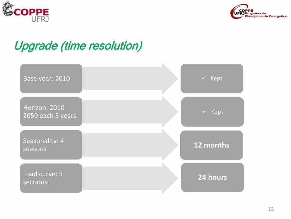
Upgrade (time resolution)
Base year: 2010
Horizon: 2010-2050 each 5 years
Seasonality: 4 seasons
Load curve: 5 sections
Kept
Kept
12 months
24 hours
13
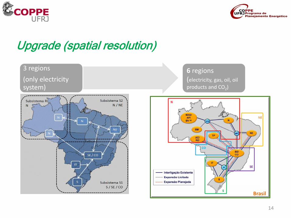
Upgrade (spatial resolution)
3 regions
(only electricitysystem)
6 regions(electricity, gas, oil, oil
products and CO2)
Brasil
14
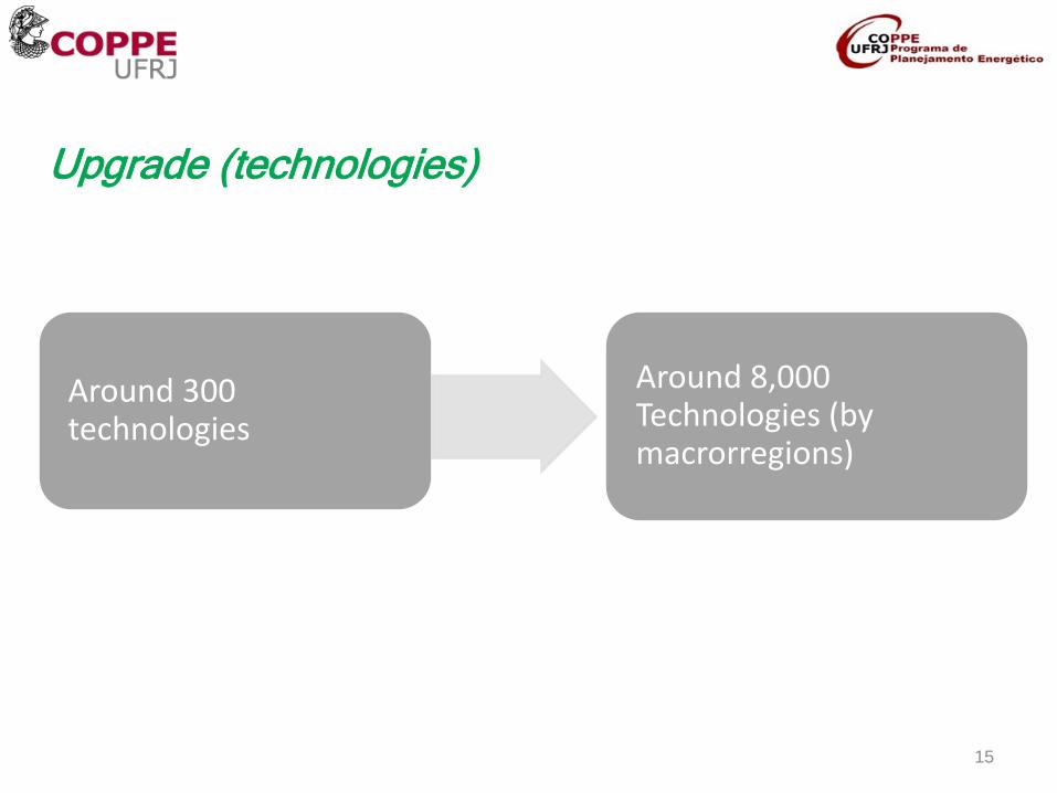
Upgrade (technologies)
Around 300 technologies
Around 8,000 Technologies (bymacrorregions)
15
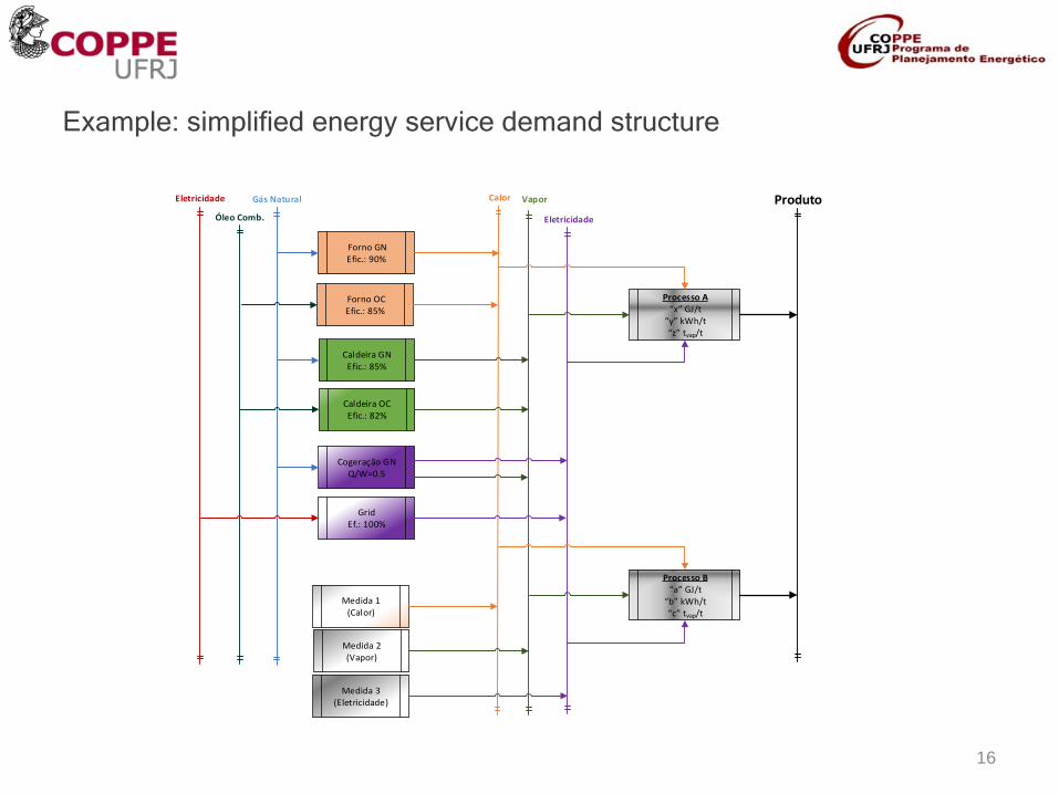
Example: simplified energy service demand structure
Forno GNEfic.: 90%
Gás Natural Calor
Caldeira GNEfic.: 85%
Vapor
Óleo Comb.
Forno OCEfic.: 85%
Caldeira OCEfic.: 82%
Eletricidade
Eletricidade
Cogeração GNQ/W=0.5
GridEf.: 100%
Processo A x GJ/t
y kWh/t z tvap/t
Processo B a GJ/t
b kWh/t c tvap/t
Produto
Medida 1(Calor)
Medida 2(Vapor)
Medida 3(Eletricidade)
16
Ministry Of Science and Technology/ PNUMA/ GEF
Project "Mitigation Options of Greenhouse Gas (GHG)
Emissions in Key Sectors in Brazil“
A full hybrid integrated model to support Brazil´s NDC
Consistency (Energy-Economy-Land Use)
All simulations and iterative procedures done!
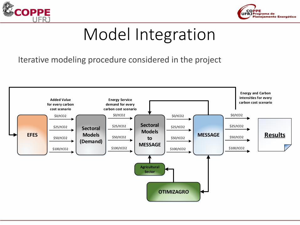
Model IntegrationIterative modeling procedure considered in the project
EFESSectoral Models
(Demand)
Sectoral Models
to MESSAGE
MESSAGE
Agricultural Sector
OTIMIZAGRO
$0/tCO2
$25/tCO2
$50/tCO2
$100/tCO2
$0/tCO2
$25/tCO2
$50/tCO2
$100/tCO2
$0/tCO2
$25/tCO2
$50/tCO2
$100/tCO2
$0/tCO2
$25/tCO2
$50/tCO2
$100/tCO2
Added Valuefor every carbon
cost scenario
Energy Service demand for every
carbon cost scenario
Energy and Carbon intensities for every carbon cost scenario
Results
Few and not so fresh results presented in Morocco(Nov 2016):
Results: consistent, integrated, detailed by usefulenergy or industrial process.. As you wish
(for more details, please see: http://www.mct.gov.br/upd_blob/0240/240525.pdf)
19
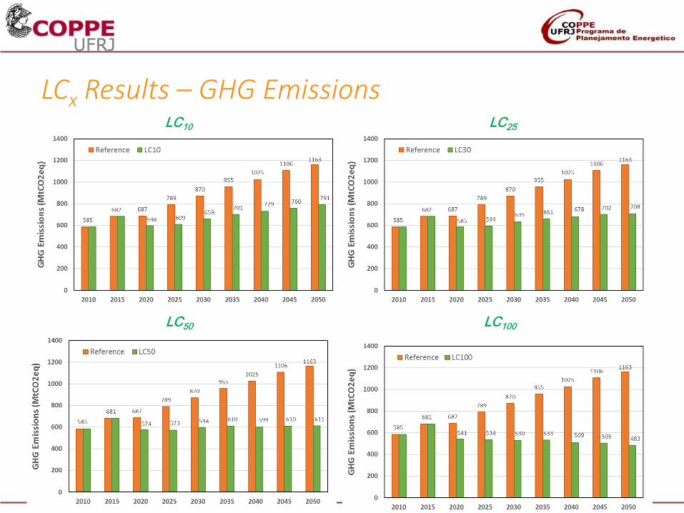
LCx Results – GHG EmissionsLC10
LC50 LC100
LC25
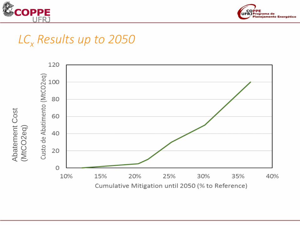
LCx Results up to 2050
Abate
ment C
ost
(MtC
O2eq)
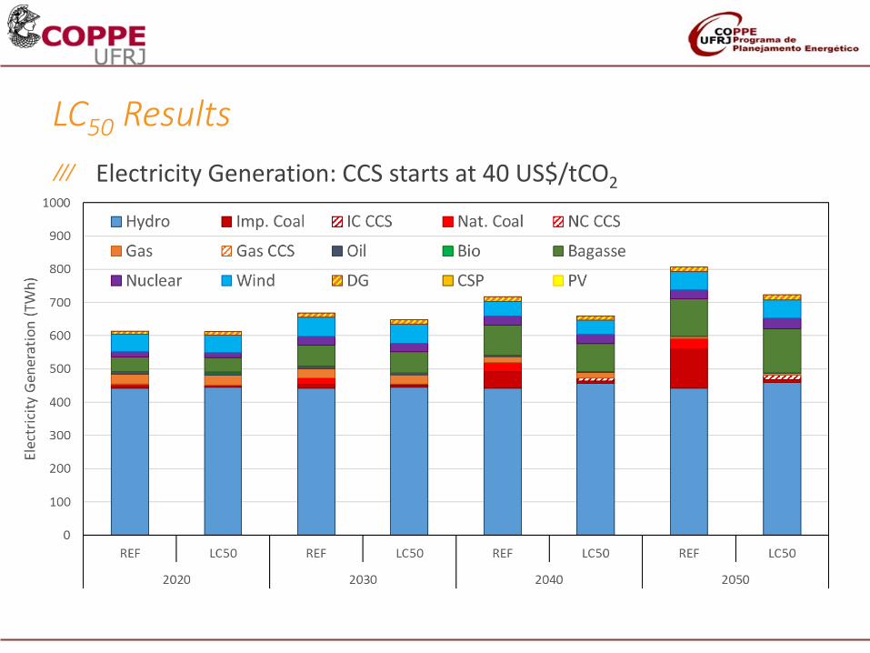
LC50 Results
Electricity Generation: CCS starts at 40 US$/tCO2
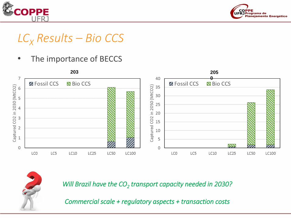
LCX Results – Bio CCS
Will Brazil have the CO2 transport capacity needed in 2030?
Commercial scale + regulatory aspects + transaction costs
203
0
• The importance of BECCS
205
0
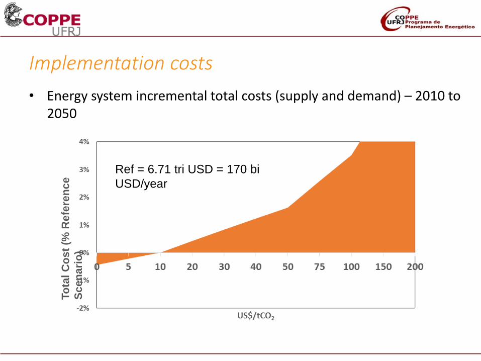
Implementation costs
Ref = 6.71 tri USD = 170 bi
USD/year
To
tal
Co
st
(% R
efe
ren
ce
Sc
en
ari
o)
• Energy system incremental total costs (supply and demand) – 2010 to 2050
Our Global IAM
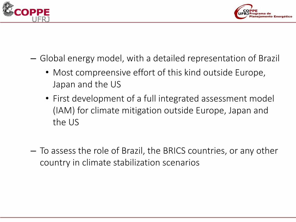
– Global energy model, with a detailed representation of Brazil
• Most compreensive effort of this kind outside Europe, Japan and the US
• First development of a full integrated assessment model (IAM) for climate mitigation outside Europe, Japan and the US
– To assess the role of Brazil, the BRICS countries, or any othercountry in climate stabilization scenarios
COFFEE (COppe´s integrated assessment Framework For Energy, land and the Environment)
A GLOBAL INTEGRATED MODEL
Alexandre Szklo and Roberto Schaeffer
With sincere thanks to Pedro Rochedo, the lead developer of this model, and from whom we have adapted these slides,
borrowed from his doctoral dissertation defense
Full version originally presente in EPE, November 9th 2016
• RCP
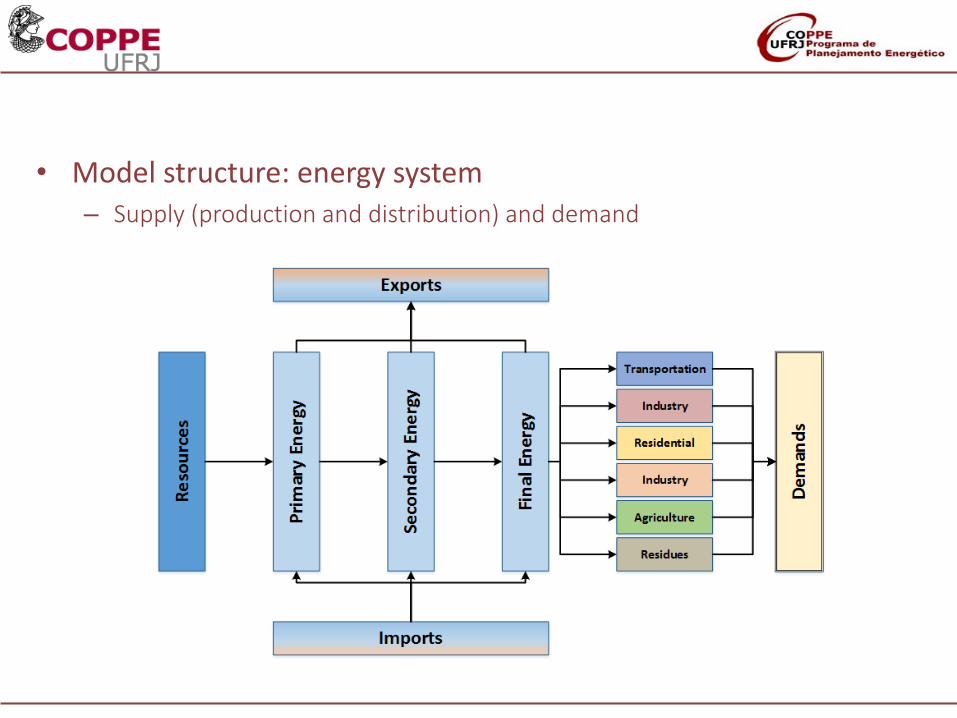
• Model structure: energy system– Supply (production and distribution) and demand
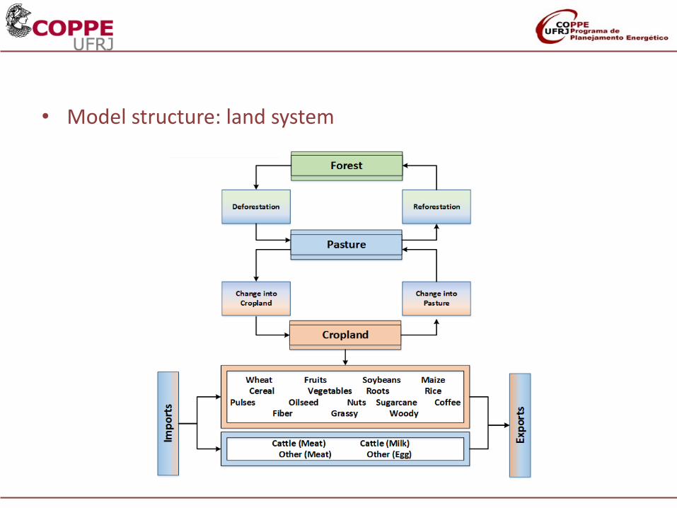
• Model structure: land system
• Oil
– Detailed representation of resources, discovered and to be discovered• Split by category and type (on/offshore)
– 18 categories per region• 324 resources with associated gas
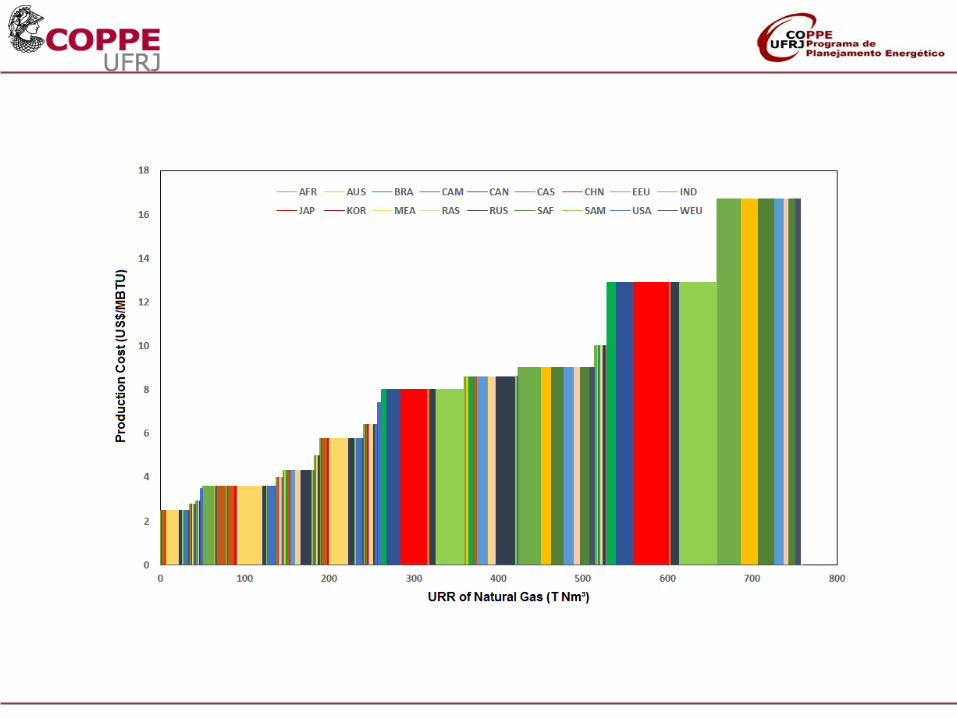
• Natural gas
– Additional detail on non-associated gas• Including shale gas (non-conventional)
– 14 categories per region• 252 resources, most of them including estimates on liquids (LNG)
• Coal
– 3 types (betuminous, sub-betuminous and lignite)
– 19 categories per region• 342 resources, with estimates for open and underground mining, including coal-bed methane
Energy resources
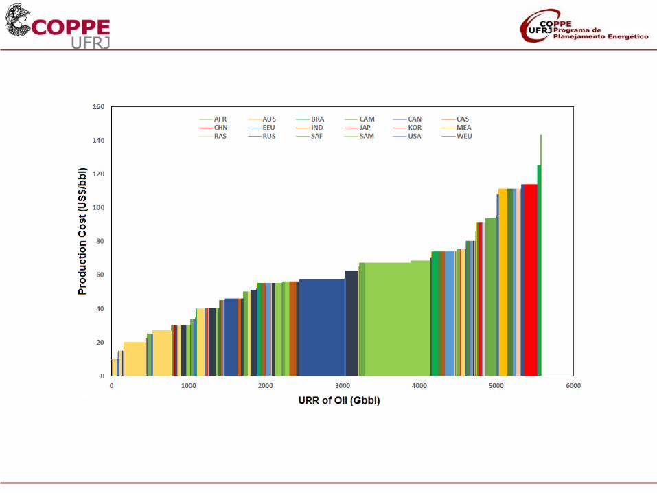
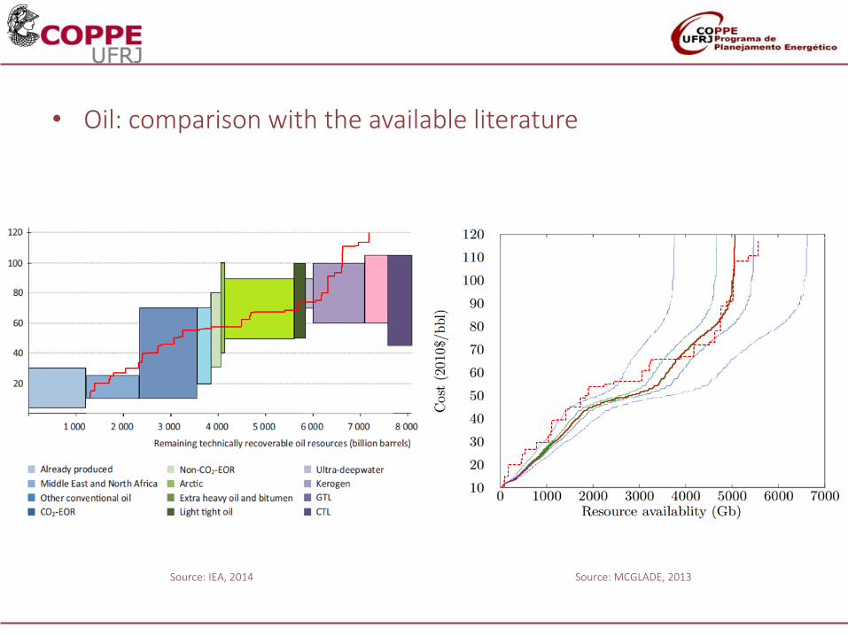
• Oil: comparison with the available literature
Source: IEA, 2014 Source: MCGLADE, 2013
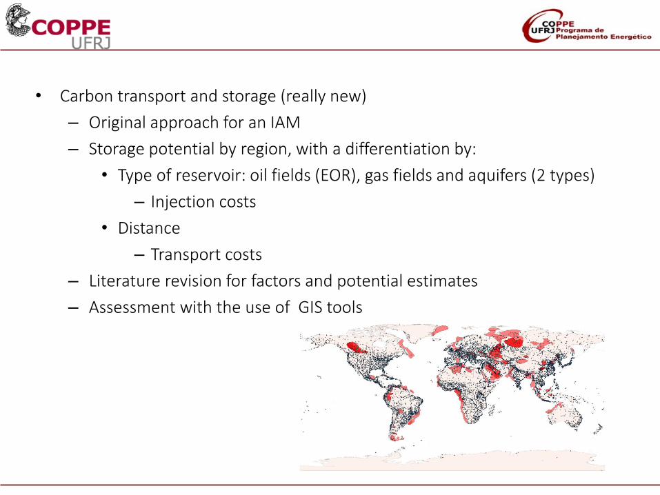
• Carbon transport and storage (really new)
– Original approach for an IAM
– Storage potential by region, with a differentiation by:
• Type of reservoir: oil fields (EOR), gas fields and aquifers (2 types)
– Injection costs
• Distance
– Transport costs
– Literature revision for factors and potential estimates
– Assessment with the use of GIS tools
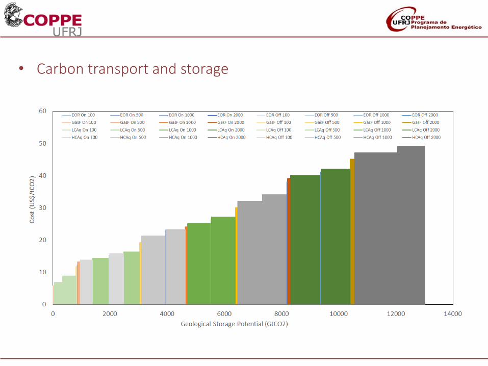
• Carbon transport and storage
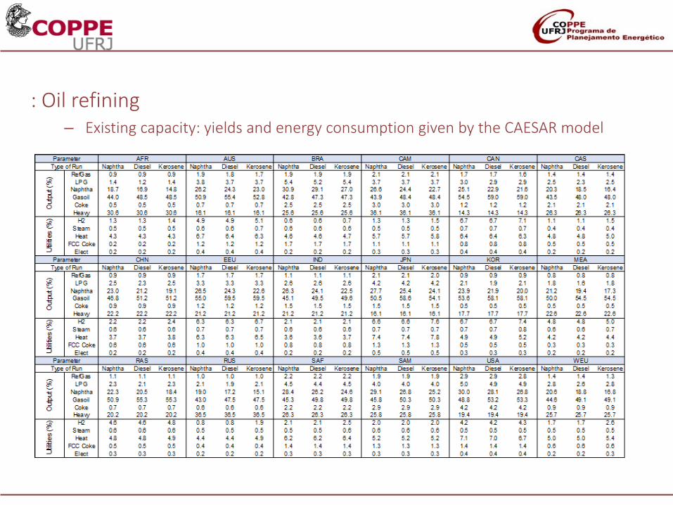
: Oil refining– Existing capacity: yields and energy consumption given by the CAESAR model
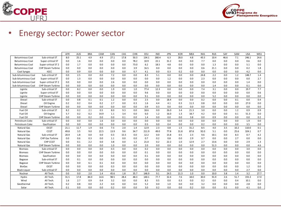
• Energy sector: Power sector
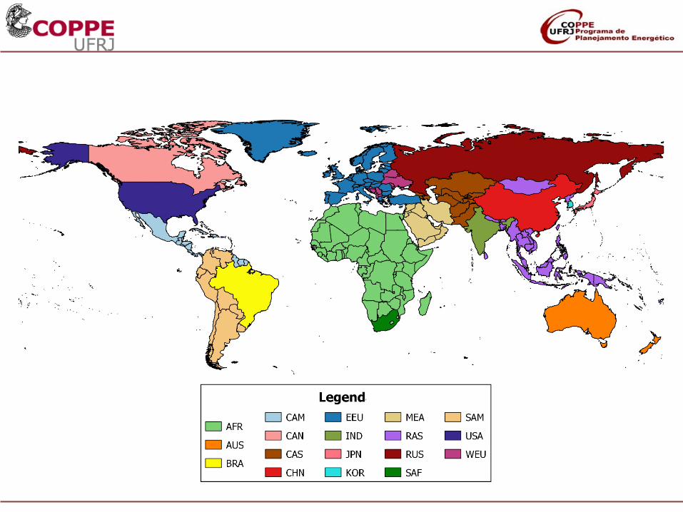
AFR AUS BRA CAM CAN CAS CHN EEU IND JPN KOR MEA RAS RUS SAF SAM USA WEU
Betuminous Coal Sub-critical ST 8.0 25.1 4.9 4.9 27.1 17.8 50.3 134.1 260.4 6.3 28.0 4.8 45.5 10.4 46.6 7.1 246.1 24.6
Betuminous Coal Super-critical ST 0.0 1.6 0.0 0.0 0.0 0.0 78.2 10.9 22.1 31.2 0.0 0.0 7.7 0.0 0.0 0.0 0.6 0.0
Betuminous Coal Super-critical ST 2 0.0 1.7 0.0 0.0 0.0 0.0 73.0 6.2 18.5 4.8 0.0 0.0 0.0 1.3 0.0 0.0 5.1 0.0
Betuminous Coal CHP Steam Turbine 0.0 0.0 0.0 0.0 0.0 0.0 3.9 16.5 0.0 0.0 0.0 0.0 0.6 21.1 0.0 0.0 0.2 1.8
Coal Syngas IGCC 0.0 0.9 0.0 0.0 0.0 0.0 0.7 4.1 0.0 0.3 0.2 0.0 0.0 0.0 0.0 0.0 4.2 0.0
Sub-bituminous Coal Sub-critical ST 0.0 2.5 0.0 0.0 7.2 0.0 0.0 8.3 5.1 0.0 0.0 0.0 24.8 2.2 0.0 1.2 148.7 1.4
Sub-bituminous Coal Super-critical ST 0.0 1.3 0.0 0.0 0.0 0.0 0.0 0.0 0.0 1.2 0.0 0.0 2.3 0.0 0.0 0.0 0.0 2.7
Sub-bituminous Coal Super-critical ST 2 0.0 0.0 0.0 0.0 2.6 0.0 0.0 0.0 0.0 0.0 0.0 0.0 0.0 0.0 0.0 0.0 1.4 0.0
Sub-bituminous Coal CHP Steam Turbine 0.0 0.0 0.0 0.0 0.0 0.0 0.0 0.0 0.0 0.0 0.0 0.0 0.0 1.4 0.0 0.0 0.1 0.0
Lignite Sub-critical ST 0.0 8.2 0.0 0.0 1.9 0.0 1.0 77.4 12.3 0.0 0.0 0.0 7.4 3.1 0.0 0.0 19.7 7.7
Lignite Super-critical ST 0.0 0.0 0.0 0.0 0.0 0.0 0.0 9.6 0.0 0.0 0.0 0.0 0.0 0.0 0.0 0.0 0.0 0.6
Lignite CHP Steam Turbine 0.0 0.0 0.0 0.0 0.0 0.0 0.0 9.1 0.0 0.0 0.0 0.0 0.0 5.2 0.0 0.0 0.0 0.0
Diesel Sub-critical ST 0.0 0.8 0.1 0.1 1.2 0.0 0.0 2.5 0.0 18.4 0.0 0.0 0.2 0.0 0.0 0.1 0.0 0.4
Diesel Oil Engine 0.2 0.2 0.4 0.2 2.7 0.0 0.3 1.6 4.4 4.1 0.3 11.3 0.8 0.0 0.0 0.0 27.0 0.0
Diesel CHP Steam Turbine 0.0 0.0 0.0 0.0 0.0 0.0 0.0 0.9 0.3 0.0 0.0 0.0 0.0 0.0 0.0 0.0 0.0 0.0
Fuel Oil Sub-critical ST 8.2 0.2 2.1 0.5 8.0 9.3 0.0 18.6 0.0 26.0 3.4 21.3 3.0 0.0 0.0 1.2 0.9 0.9
Fuel Oil Oil Engine 5.7 0.2 0.2 14.9 1.1 3.4 0.0 6.0 1.2 16.0 1.3 18.7 4.2 0.0 0.0 0.1 51.3 0.0
Fuel Oil CHP Steam Turbine 0.0 0.0 0.2 0.0 0.0 0.1 0.0 1.4 0.0 0.0 0.0 3.8 0.0 0.9 0.0 0.0 0.0 0.2
Petroleum Coke Sub-critical ST 0.0 0.0 0.0 1.6 0.0 0.0 0.0 0.0 0.0 0.0 0.0 0.0 0.0 0.0 0.0 0.0 1.9 0.0
Petroleum Coke Gasification 0.0 0.0 0.0 0.0 0.0 0.0 0.0 0.3 0.0 0.4 0.0 0.0 0.2 0.0 0.0 0.0 3.5 0.0
Natural Gas OCGT 21.1 11.7 1.9 0.6 7.3 2.0 1.4 12.9 2.3 0.8 1.5 31.2 8.5 4.0 3.5 10.2 110.0 0.1
Natural Gas CCGT 49.8 3.5 9.0 22.5 13.9 9.6 34.7 211.9 49.0 77.8 31.8 87.8 92.0 5.1 0.0 25.6 324.1 0.7
Natural Gas Sub-critical ST 20.9 1.8 0.0 0.0 0.3 15.5 0.0 12.2 0.0 15.8 0.5 2.3 9.6 10.1 0.0 8.3 0.7 4.2
Natural Gas CHP Gas Turbine 0.0 0.6 0.3 0.0 1.1 0.0 0.0 0.7 0.2 0.8 0.0 2.9 0.7 0.0 0.0 2.7 0.0 0.0
Natural Gas CHP CCGT 0.0 0.1 2.2 0.0 3.8 0.0 1.2 21.0 0.2 22.2 1.0 12.9 2.7 13.6 0.0 0.0 2.9 1.3
Natural Gas CHP Steam Turbine 0.0 0.0 0.0 0.0 1.0 0.0 0.0 2.0 0.0 0.0 0.0 0.0 0.0 51.3 0.0 0.0 0.0 4.6
Biomass Sub-critical ST 0.0 0.0 0.0 0.0 0.3 0.0 0.0 0.2 0.0 0.0 0.0 0.0 0.0 0.0 0.0 0.0 3.0 0.0
Biomass CHP Steam Turbine 0.0 0.0 0.0 0.0 0.0 0.0 0.0 0.1 0.0 0.0 0.0 0.0 0.0 0.0 0.0 0.0 0.0 0.0
Biomass Gasification 0.0 0.0 0.0 0.0 0.0 0.0 0.0 0.1 0.0 0.0 0.0 0.0 0.0 0.0 0.0 0.0 0.0 0.0
Bagasse Sub-critical ST 0.0 0.1 0.0 0.0 0.0 0.0 0.0 0.0 0.0 0.0 0.0 0.0 0.0 0.0 0.0 0.0 0.0 0.0
Bagasse CHP Steam Turbine 0.0 0.0 6.1 0.1 0.0 0.0 0.0 0.0 0.0 0.0 0.0 0.0 0.0 0.0 0.0 0.0 0.0 0.0
BioGas OCGT 0.0 0.0 0.0 0.0 0.3 0.0 0.0 0.0 0.0 0.0 0.0 0.0 0.0 0.0 0.0 0.0 1.2 0.0
Black Liquor Sub-critical ST 0.0 0.0 0.0 0.0 0.0 0.0 0.0 0.0 0.0 0.0 0.0 0.0 0.0 0.0 0.0 0.0 2.7 0.0
Nuclear All Tech. 0.0 0.0 2.0 1.4 45.6 1.8 35.7 146.9 9.1 24.5 21.3 1.0 0.0 10.0 3.8 1.4 3.2 27.7
Hydro All Tech. 31.5 17.8 84.0 14.6 98.5 28.4 48.3 140.1 77.7 32.4 7.6 18.0 30.0 91.9 2.6 51.7 155.3 17.0
Wind All Tech. 1.6 2.7 0.9 0.4 3.2 0.0 0.0 8.3 0.5 0.0 0.3 0.0 0.2 0.0 0.0 0.4 10.1 0.0
Geothermal All Tech. 0.2 0.8 0.0 2.2 0.0 0.0 0.0 5.2 0.0 1.0 0.0 0.0 3.2 0.0 0.0 0.0 2.8 0.0
Solar All Tech. 0.1 0.0 0.0 0.0 0.2 0.0 0.0 3.0 0.2 0.0 0.0 0.2 0.0 0.0 0.1 0.0 4.1 0.0
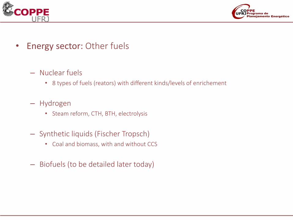
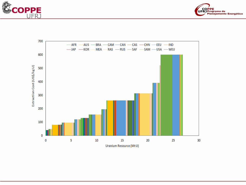
• Energy sector: Other fuels
– Nuclear fuels• 8 types of fuels (reators) with different kinds/levels of enrichement
– Hydrogen• Steam reform, CTH, BTH, electrolysis
– Synthetic liquids (Fischer Tropsch)• Coal and biomass, with and without CCS
– Biofuels (to be detailed later today)
• End-use sectors
– Transport
– Industry
– Residential
– Services (excluding Transport)
– Residues
– Agriculture
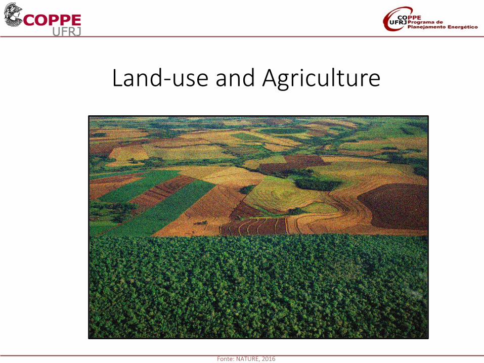
Land-use and Agriculture
Fonte: NATURE, 2016
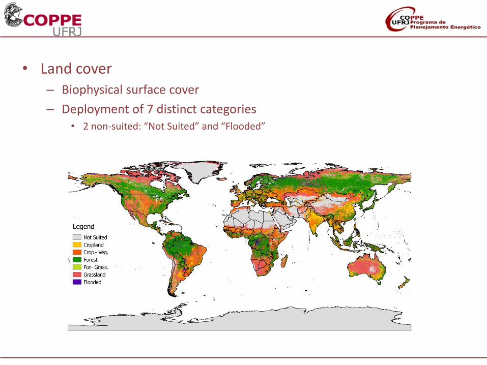
• Land cover– Biophysical surface cover
– Deployment of 7 distinct categories• 2 non-suited: “Not Suited” and “Flooded”
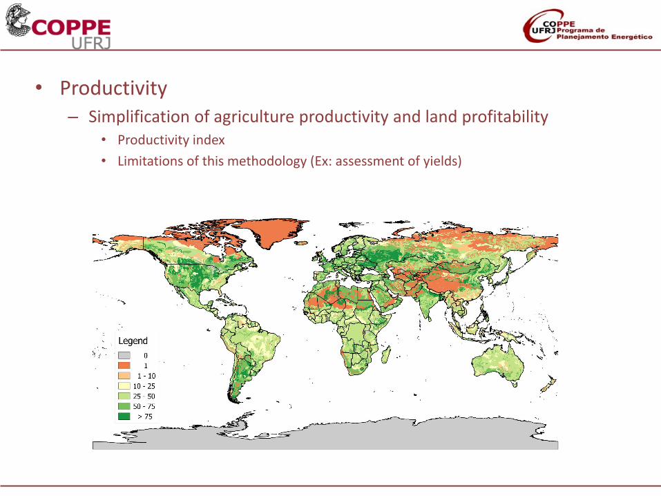
• Productivity– Simplification of agriculture productivity and land profitability
• Productivity index
• Limitations of this methodology (Ex: assessment of yields)
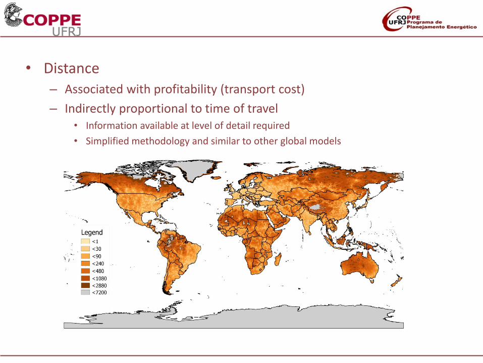
• Distance– Associated with profitability (transport cost)
– Indirectly proportional to time of travel• Information available at level of detail required
• Simplified methodology and similar to other global models
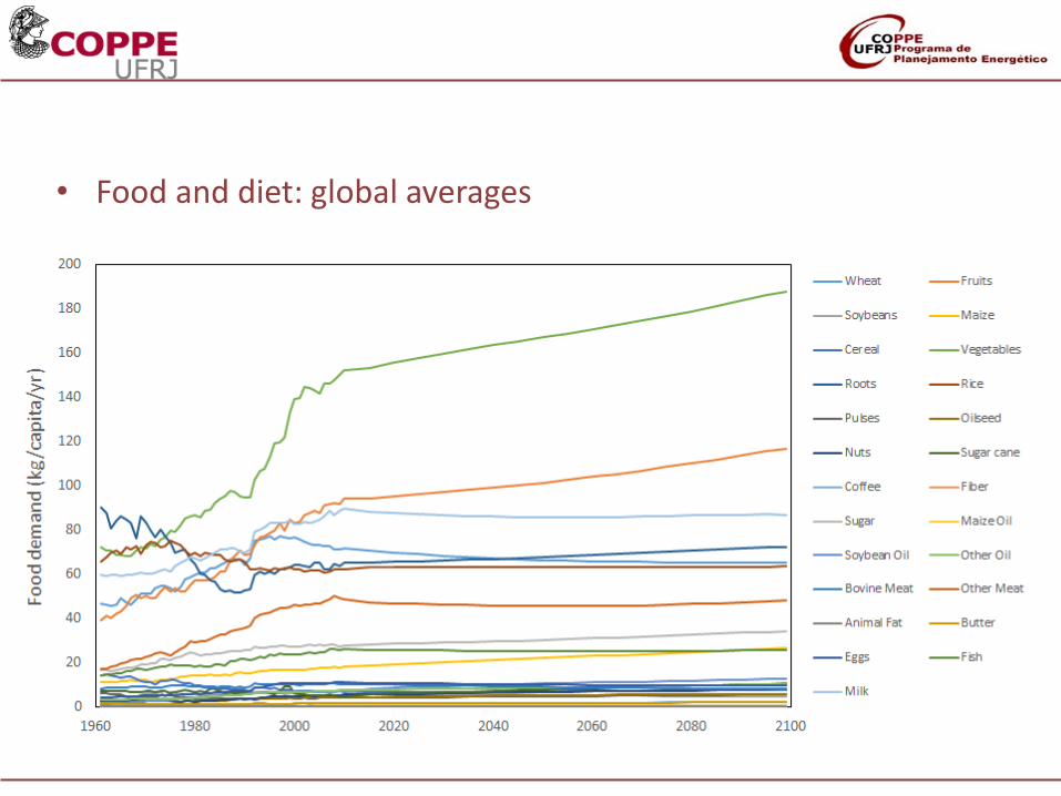
• Food and diet: global averages
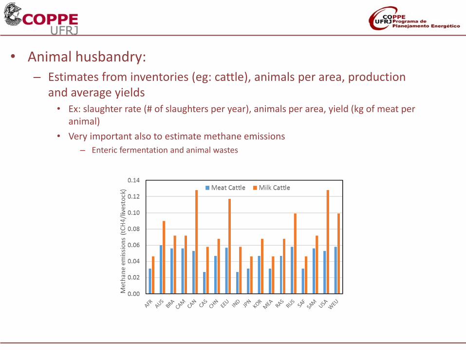
• Animal husbandry:– Estimates from inventories (eg: cattle), animals per area, production
and average yields• Ex: slaughter rate (# of slaughters per year), animals per area, yield (kg of meat per
animal)
• Very important also to estimate methane emissions
– Enteric fermentation and animal wastes
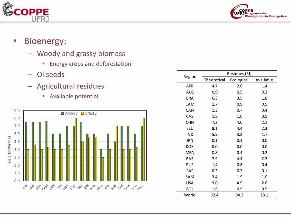
• Bioenergy:– Woody and grassy biomass
• Energy crops and deforestation
– Oilseeds
– Agricultural residues• Available potential
Theoretical Ecological Available
AFR 4.7 2.6 1.4
AUS 0.9 0.5 0.3
BRA 6.3 3.5 1.8
CAM 1.7 0.9 0.5
CAN 1.3 0.7 0.4
CAS 1.8 1.0 0.5
CHN 7.2 4.0 2.1
EEU 8.1 4.4 2.3
IND 5.9 3.2 1.7
JPN 0.1 0.1 0.0
KOR 0.0 0.0 0.0
MEA 0.8 0.4 0.2
RAS 7.9 4.4 2.3
RUS 1.4 0.8 0.4
SAF 0.3 0.2 0.1
SAM 3.4 1.9 1.0
USA 9.0 4.9 2.6
WEU 1.6 0.9 0.5
World 62.4 34.3 18.1
Residues (EJ)Region
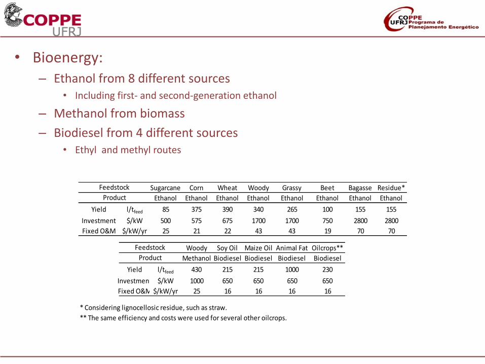
• Bioenergy:– Ethanol from 8 different sources
• Including first- and second-generation ethanol
– Methanol from biomass
– Biodiesel from 4 different sources• Ethyl and methyl routes
Sugarcane Corn Wheat Woody Grassy Beet Bagasse Residue*
Ethanol Ethanol Ethanol Ethanol Ethanol Ethanol Ethanol Ethanol
Yield l/tfeed 85 375 390 340 265 100 155 155
Investment $/kW 500 575 675 1700 1700 750 2800 2800
Fixed O&M $/kW/yr 25 21 22 43 43 19 70 70
Woody Soy Oil Maize Oil Animal Fat Oilcrops**
Methanol Biodiesel Biodiesel Biodiesel Biodiesel
Yield l/tfeed 430 215 215 1000 230
Investment $/kW 1000 650 650 650 650
Fixed O&M $/kW/yr 25 16 16 16 16
** The same efficiency and costs were used for several other oilcrops.
* Considering lignocellosic residue, such as straw.
Feedstock
Product
Product
Feedstock
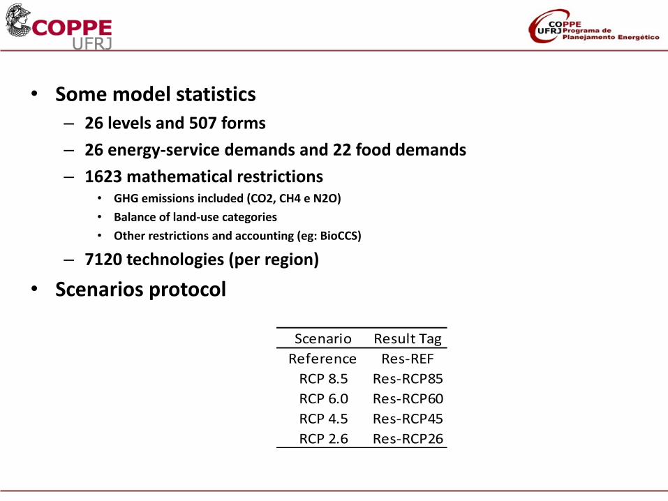
• Some model statistics– 26 levels and 507 forms
– 26 energy-service demands and 22 food demands
– 1623 mathematical restrictions• GHG emissions included (CO2, CH4 e N2O)
• Balance of land-use categories
• Other restrictions and accounting (eg: BioCCS)
– 7120 technologies (per region)
• Scenarios protocol
Scenario Result Tag
Reference Res-REF
RCP 8.5 Res-RCP85
RCP 6.0 Res-RCP60
RCP 4.5 Res-RCP45
RCP 2.6 Res-RCP26
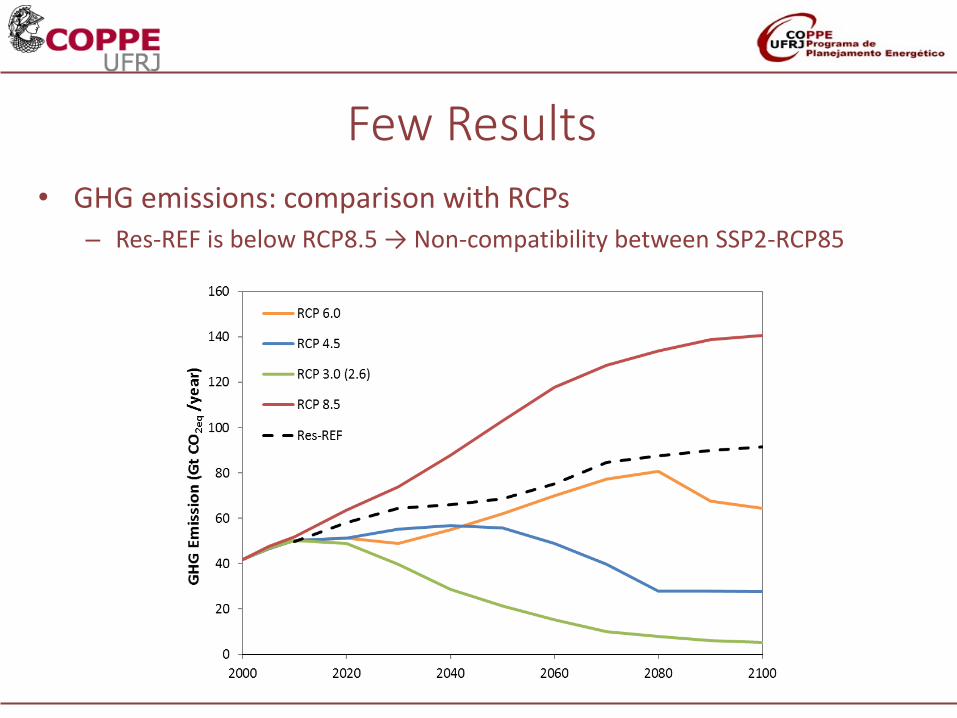
• GHG emissions: comparison with RCPs– Res-REF is below RCP8.5 → Non-compatibility between SSP2-RCP85
Few Results
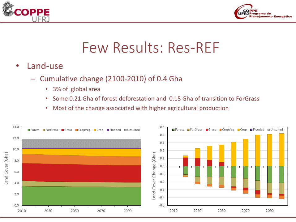
• Land-use– Cumulative change (2100-2010) of 0.4 Gha
• 3% of global area
• Some 0.21 Gha of forest deforestation and 0.15 Gha of transition to ForGrass
• Most of the change associated with higher agricultural production
Few Results: Res-REF
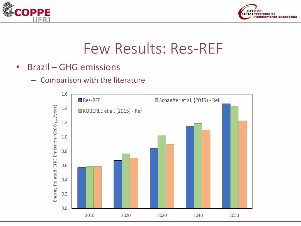
• Brazil – GHG emissions– Comparison with the literature
Few Results: Res-REF
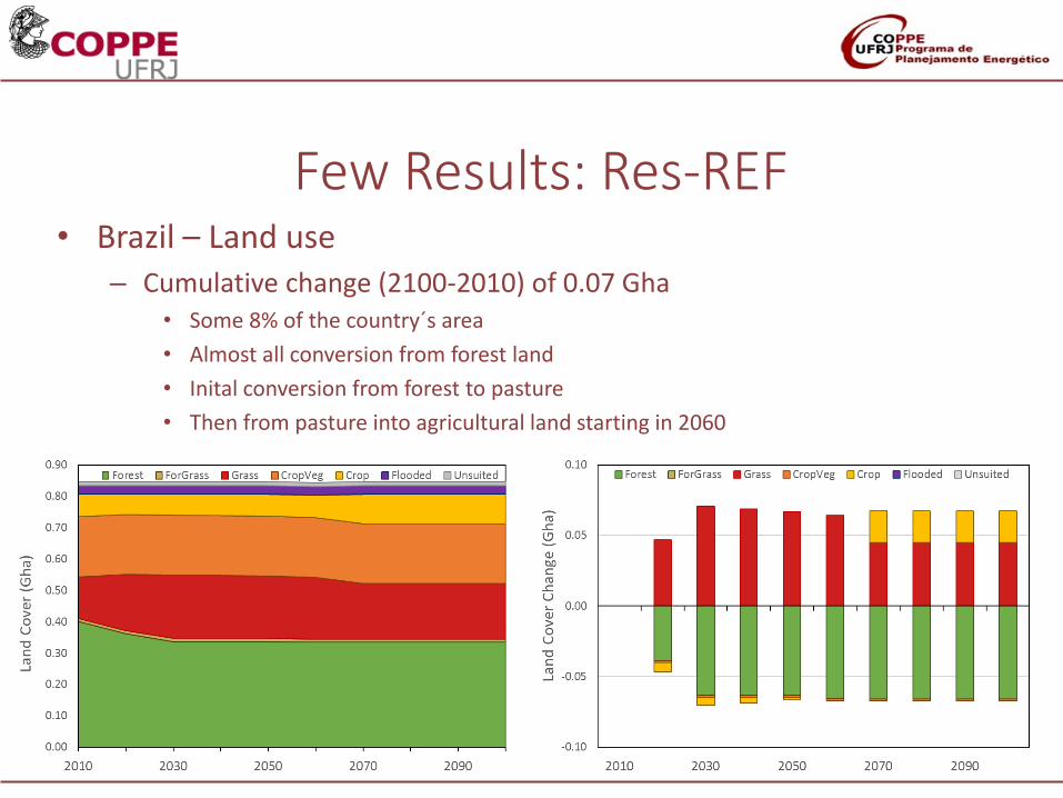
• Brazil – Land use– Cumulative change (2100-2010) of 0.07 Gha
• Some 8% of the country´s area
• Almost all conversion from forest land
• Inital conversion from forest to pasture
• Then from pasture into agricultural land starting in 2060
Few Results: Res-REF
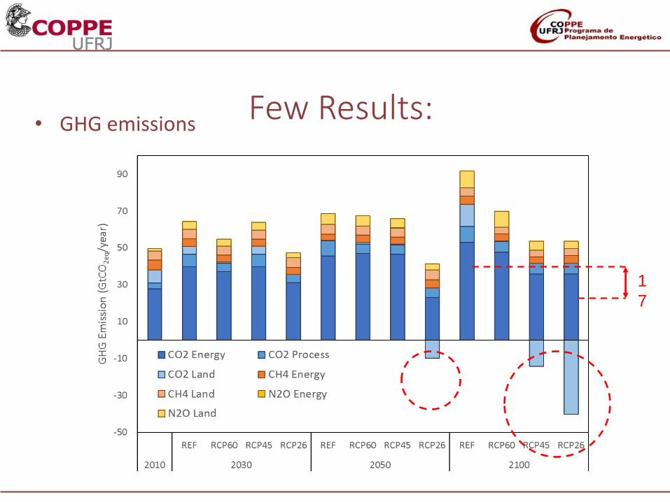
• GHG emissionsFew Results:
1
7
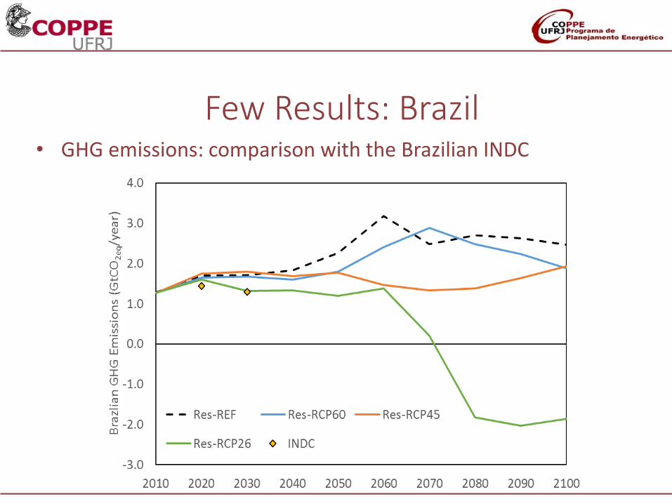
• GHG emissions: comparison with the Brazilian INDC
Few Results: Brazil
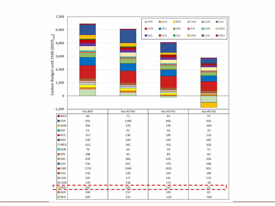
58
What next?
• Incorporation of water nexus
• How cost overruns in energy megaprojects lead to suboptimal decisions in energy sector planning
• This is because our research is showing an increase in overnight construction costs (OCC) and lead time escalations for energy megaprojects over time
59
• Global Integrated energy Model (COFFEE) + Global CGE model (TEA): up to June 2017
• Incorporation of a simple Climate Model intoCOFFEE, so as to move from GHG emissions, to GHG concentration, radiative forcings and temperature increase: up to August 2018
• To be continued ...