MODELING FISCHER-TROPSCH PRODUCT DISTRIBUTION OF A COBALT

BASED CATALYST IN DIFFERENT REACTION MEDIA

A Thesis

by

SHAIK AFZAL

Submitted to the Office of Graduate and Professional Studies of

Texas A&M University

in partial fulfillment of the requirements for the degree of

MASTER OF SCIENCE

Chair of Committee, Nimir O. Elbashir

Committee Members, Marcelo Castier

Hazem Nounou

Head of Department, M. Nazmul Karim

August 2015

Major Subject: Chemical Engineering

Copyright 2015 Shaik Afzal

ii

ABSTRACT

This work discusses the modeling of hydrocarbon product distribution up to carbon

number 15 of a cobalt-based catalyst under Fischer-Tropsch (FT) synthesis

conditions. The proposed kinetics of the reaction has been adapted from Todic et al.

In the first part of the study, a Genetic Algorithm code in MATLAB® was developed

to generate parameters of the 19-parameter kinetic model. In the next part of the work,

an experimental campaign was conducted in a high pressure FT reactor unit to verify

the model predictability of the cobalt catalyst product profile in gas phase. The results

in terms of conversion and hydrocarbon product formations were reported. Less than

12% CO conversion was maintained in all 7 runs in order to ensure that the reaction

was occurring in the kinetic regime. After the peak identification and analysis, the

experimental data was input into the developed MATLAB® code to estimate model

parameters. This model estimates the FT product distribution in the gas phase media

with a mean absolute relative residual (MARR) of 48.44%. This is higher than that

obtained by Todic et al. The higher error is attributed to the fewer number of

experimental runs carried out and due to some assumptions made in product

characterization. This work lays the foundation for future work towards investigations

of FT product distribution in the presence of a supercritical solvent to bring the

reaction media to near critical and supercritical phase conditions.

iii

DEDICATION

Dedicated to my family

iv

ACKNOWLEDGMENTS

In the name of God, Most Gracious, Most Merciful.

I would like to thank my committee chair, Dr. Nimir Elbashir for his consistent

and unwavering support throughout the course of this research. I thank my committee

members, Dr. Hazem Nounou, Dr. Marcelo Castier for their guidance and support during

the course of this research.

Thanks also go to my friends and colleagues and the department faculty and staff

for making my time at Texas A&M University at Qatar a great experience. I also want to

extend my gratitude to Jan Blank and Rehan Hussain for being there always to answer my

questions. Lastly but not the least I want to thank my dad, Ilyas, my mum, Anjum, my

sister, Ayesha and my wife, Wafa for their love and support throughout the period of my

study.

v

NOMENCLATURE

α probability of chain growth

c constant c, -ΔE/RT

n nth carbon number

r rate of reaction

k Arrhenius rate constant

K equilibrium constant

S fraction of vacant sites at catalyst surface

Pi partial pressure of ith component

T absolute temperature, K

A pre-exponential factor in Arrhenius rate

equation

R universal gas constant, 8.314 J/K/mol

ΔE activation energy

ΔH heat of reaction / adsorption (as applicable)

MARR mean absolute relative residual

vi

TABLE OF CONTENTS

Page

ABSTRACT ....................................................................................................................... ii

DEDICATION .................................................................................................................. iii

ACKNOWLEDGMENTS ................................................................................................. iv

NOMENCLATURE ........................................................................................................... v

TABLE OF CONTENTS .................................................................................................. vi

LIST OF TABLES .......................................................................................................... viii

LIST OF FIGURES ........................................................................................................... ix

CHAPTER I INTRODUCTION ....................................................................................... 1

1.1 Fischer Tropsch chemistry and the utilization of supercritical fluids in GTL

processes ......................................................................................................................... 1

1.2 Background of modeling Fischer-Tropsch reactors ................................................. 5

CHAPTER II RESEARCH OBJECTIVE ....................................................................... 15

CHAPTER III RESEARCH METHODOLOGY ............................................................ 16

3.1 Development of a kinetic model with focus on product distribution ..................... 17 3.2 Model validation ..................................................................................................... 22 3.3 Experimental setup ................................................................................................. 25 3.4 Analysis of the product distribution ....................................................................... 35

CHAPTER IV RESULTS AND DISCUSSION ............................................................. 40

4.1 Experimental results ............................................................................................... 40 4.2 Model results .......................................................................................................... 47

CHAPTER V CONCLUSION & FUTURE WORK ...................................................... 53

REFERENCES ................................................................................................................. 56

APPENDIX A REACTOR DATA ANALYSIS CALCULATIONS .............................. 63

vii

APPENDIX B CONVERGENCE OF GENETIC ALGORITHM RESULTS ................ 69

APPENDIX C DATA ANALYSIS RESULTS FOR ALL RUNS .................................. 71

viii

LIST OF TABLES

Page

Table 1 – Reaction Pathway of Carbide Mechanism from Todic et al [39] ..................... 18

Table 2 – Input Range for Model Parameters [39] ........................................................... 21

Table 3 – Comparison of GA Results with Parameters determined by Todic et al [39] .. 23

Table 4 – Experimental Conditions planned for Kinetic Study ....................................... 34

Table 5 – Details of Columns used in GC ........................................................................ 35

Table 6 – Temperature Programming for the GC ............................................................ 36

Table 7 – Experimental Results for all runs ..................................................................... 40

Table 8 – Model Results ................................................................................................... 48

ix

LIST OF FIGURES

Page

Figure 1 – Chain Growth Probability in FT .................................................................... 3

Figure 2 – Typical ASF Hydrocarbon Product Distribution ......................................... 4

Figure 3 – Non Ideal FT Product Distribution................................................................ 5

Figure 4 – Proposed Methodology for Research into FT in SCF Phase .......................... 16

Figure 5 – Validation of Genetic Algorithm Code ....................................................... 25

Figure 6 – Block Diagram of Reactor Unit ...................................................................... 28

Figure 7 – Calibration Curve for CO flow-rates .............................................................. 30

Figure 8 - Calibration Charts for CO, Syngas and H2 Flow Controllers .......................... 31

Figure 9 – Column Oven Temperature Program .............................................................. 36

Figure 11 – Identification of Olefin Peaks ....................................................................... 38

Figure 12 – Deconvolution of C3 peaks ........................................................................... 39

Figure 13 – CO Conversion % with time-on-stream ........................................................ 43

Figure 14 – CO2 Selectivity with time-on-stream ............................................................ 43

Figure 15 – CH4 Selectivity with time-on-stream ............................................................ 44

Figure 16 – Peak Area with Carbon Number for Run No. 3 ............................................ 45

Figure 17 – Hydrocarbon Formation Rates with Carbon Number for Run No. 3 ............ 46

Figure 18 – ASF Plot for Run No. 3 ................................................................................ 47

Figure 19 – Olefin-to-Paraffin Ratio with Carbon Number for Run No. 3 ...................... 47

Figure 20 – Comparison of Experimental and Model Results ......................................... 50

1

CHAPTER I

INTRODUCTION

1.1 Fischer Tropsch chemistry and the utilization of supercritical fluids in GTL

processes

The Fischer-Tropsch synthesis (FT) is the heart of the Gas-to-Liquids (GTL)

technology as it is the process by which synthesis gas (or syngas, a mixture of carbon

monoxide and hydrogen) can be converted into ultra-clean fuels and value added

chemicals [1]. Syngas can be obtained from abundant natural resources such as coal,

natural gas, and biomass. Commercially, there are three main FT reactors currently in

use by industry for large scale GTL plants, namely fixed bed, slurry bubble bed and

the fluidized bed. Shell in its Pearl GTL plant uses the multitubular fixed-bed reactor

while Oryx GTL (a joint venture between Qatar Petroleum-SASOL) employs the

slurry reactor technology. Both plants are located in Qatar. Each reactor has its own

advantages and limitations.

The Fischer-Tropsch reaction is a heterogeneous chemical reaction in which

syngas is converted into a range of hydrocarbon products of varying carbon numbers

including condensate, middle distillate and long chain hydrocarbon waxes. These

waxes may further be cracked to produce molecules of the desired carbon lengths for

the production of ultra-clean fuels (gasoline, jet fuels and diesel) besides value-added

chemicals and lubricants. FT has gained importance among the scientific and

industrial community in the past few decades due to the increased costs of crude oil

in global markets. The process is an excellent way for countries to monetize their gas

2

reserves and diversify their businesses into the international liquid fuels and chemicals

market.

The current research is aimed at studying fixed-bed FT reactors that operate

under non-conventional reaction media through the use of supercritical fluid solvents.

This unique reaction medium leverages certain advantages of the current commercial

technologies while at the same time overcoming several of their major limitations [2].

With diffusivities that are higher than normal liquids and viscosities that are lower

than their liquid counterparts, supercritical solvents have gained importance as media

for chemical reactions due to their inherent transport properties [3].

The use of supercritical fluids for FT was first reported by Kaoru Fujimoto’s

group at the University of Tokyo in 1989 [4], many researchers reported higher

catalyst activity and better FT performance in the presence of a solvent at the near

critical and supercritical phase conditions [5-8]. Several studies have proved that the

solvent medium affects the secondary reactions taking place on the catalyst surface in

FT and hence plays a role in the chain growth process thereby influencing the overall

product distribution [5, 9-12].

In a previous study, our team reported the development of FT fixed bed reactor

model based on evaluation of the micro and macro reactor bed performance while

simultaneously accounting for the reactor bed heat and mass transfer behaviors [13].

The temperature and concentration profiles of the reactants inside the catalyst pores

and throughout the reactor bed have been accounted for [14].

3

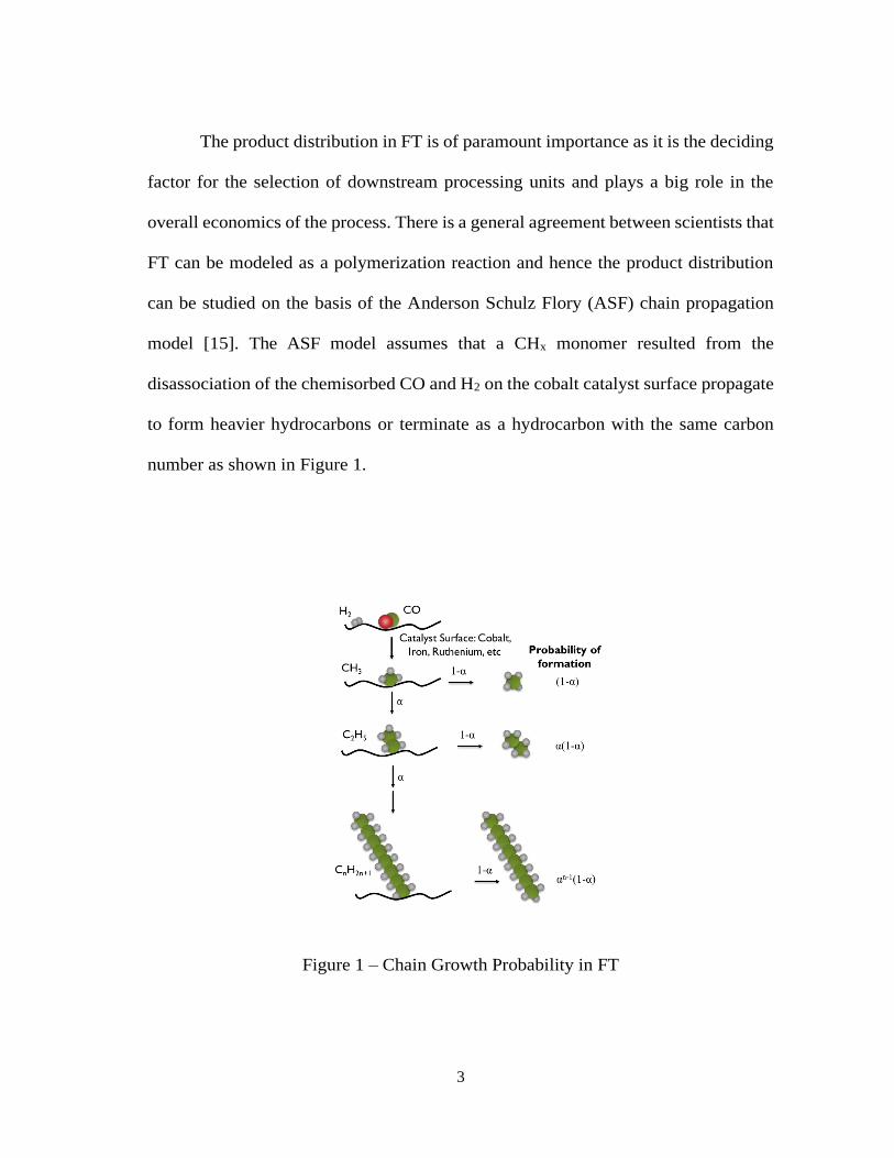
The product distribution in FT is of paramount importance as it is the deciding

factor for the selection of downstream processing units and plays a big role in the

overall economics of the process. There is a general agreement between scientists that

FT can be modeled as a polymerization reaction and hence the product distribution

can be studied on the basis of the Anderson Schulz Flory (ASF) chain propagation

model [15]. The ASF model assumes that a CHx monomer resulted from the

disassociation of the chemisorbed CO and H2 on the cobalt catalyst surface propagate

to form heavier hydrocarbons or terminate as a hydrocarbon with the same carbon

number as shown in Figure 1.

Figure 1 – Chain Growth Probability in FT

4

The chain growth probability α in the ASF model is assumed to be independent

of the carbon number and temperature. The FT hydrocarbon product profile for various

values of α is shown below in Figure 2.

Figure 2 – Typical ASF Hydrocarbon Product Distribution

Several studies reported experimental data of FT product distribution that deviate

from the ASF plot [16, 17]. A number of researchers accounted for this deviation by

assuming multiple chain growth values (α-values) [17-19].

The deviation from standard ASF has also been observed in FT reactions in

supercritical phase medium [18]. The solvent phase could influence chain growth

pathway by suppressing methanation and favoring formation of olefins and long chains,

which could result in deviation from ASF plot [18].

0

0.1

0.2

0.3

0.4

0.5

0.6

0.7

0.8

0.9

1

0.2 0.4 0.6 0.8 1

Weig

ht

Fra

ctio

n

Probability of Chain Growth, α

Light Hydrocarbons, C1-C4

Gasoline, C5-C10

Jet Fuel/Diesel, C11-C19

Wax, C20+

5

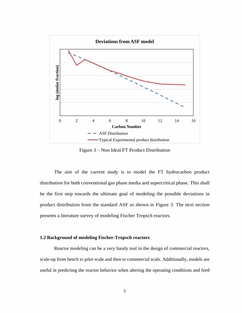
Figure 3 – Non Ideal FT Product Distribution

The aim of the current study is to model the FT hydrocarbon product

distribution for both conventional gas phase media and supercritical phase. This shall

be the first step towards the ultimate goal of modeling the possible deviations in

product distribution from the standard ASF as shown in Figure 3. The next section

presents a literature survey of modeling Fischer Tropsch reactors.

1.2 Background of modeling Fischer-Tropsch reactors

Reactor modeling can be a very handy tool in the design of commercial reactors,

scale-up from bench to pilot scale and then to commercial scale. Additionally, models are

useful in predicting the reactor behavior when altering the operating conditions and feed

0 2 4 6 8 10 12 14 16

log

(m

ola

r fr

act

ion

)

Carbon Number

Deviations from ASF model

ASF Distribution

Typical Experimental product distribution

6

composition. Developing a comprehensive model that is capable of predicting the Fischer-

Tropsch reaction performance (conversion, selectivity) while simultaneously account for

the heat and mass transfer behavior inside the reactor bed is a quite complex mission since

this reaction involves complex mechanisms for hundreds of reactions take place at the

catalyst surface [20].

Furthermore, FT is a highly exothermic reaction that could cause hot spot

formation on catalyst surface especially for the fixed-bed reactors. To control the

temperature inside these type of reactors, it is essential to measure or predict the axial and

the radial temperature profiles inside catalyst pores and in the bulk phase. The accurate

prediction or modeling of these profiles require appropriate accounting of the reaction

kinetics and thermodynamics of the FT reaction mixture, which further complicate the

modeling development process. The catalyst type and pellet properties (shape, diameter,

pore and surface characteristics) are critical parameters in controlling the FT reaction

performance and they are the starting point in developing a model for the reaction at the

micro-scale level. The comprehensive model for the FT fixed-bed reactor includes the

macro-scale level of the process as well to provide quantitative assessments of the

following: mass and heat transfer rates between the bulk fluid and the pellet outer surface

(external transfer), the inter-particle diffusion of mass and heat inside the tortuous pellet

structure (internal transfer), the rate of surface reaction and diffusing back of products and

remaining reactants from the catalyst interior pore to the surface of the catalyst pellet and

then to the bulk fluid. Producing a detailed reactor model should take into account the

aforementioned mass, heat and momentum transfer processes, which are quite challenging

7

to quantify simultaneously [21]. As the temperature influences the reaction kinetics and

chain growth process directly, tracking temperature changes in the reactor bed is crucial

to FT process safety and performance. The temperature profile inside the reactor bed

should match the measured or predicted primary and secondary reaction rates and chain

termination rates as they are intensely affected by the reactor bed temperature. Likewise

the diffusion and other physical properties controlling the reaction rate are strongly

dependent on temperature. In conclusion, the complexity of the mathematics associated to

the model makes the formulation of the simulation program cumbersome and time

consuming.

1.2.1 Techniques to Develop Fischer Tropsch Fixed Bed Reactor Models

Various 1-Dimensional (1-D) models have been proposed in literature for fixed

bed FT reactors. This section discusses some of these approaches. Wang et al. [22] studied

the effects of tube diameter, recycle ratio, pressure and cooling temperature on selectivity,

conversion of a Fe-Cu-K based catalyst while modeling the temperature profiles in a

jacketed FBR. The catalyst pores were assumed to be filled with wax and the gas film

mass transfer was neglected. Separate mass and energy balances were set up for bulk gas

phase and catalyst pores. They showed that increase in cooling temperatures increases

syngas conversion though suppressing C5+ content. On the other hand their findings

showed that increasing the pressure benefits both the CO conversion as well as C5+ product

yield. A promising paper on the selection of reactor type for low temperature Fischer-

Tropsch was published by Robert and Thomas [23]. They simulated various FT reactor

8

types using 1-D model and simple first order kinetics to provide a comparison in the

efficiency and the performance of these different reactors (fixed bed (trickle flow), slurry

bubble column, monolith loop (slug flow) and micro structured (film flow regime)). A

comprehensive list of equations used in each case was presented. They concluded that

slurry bubble column is far better than fixed bed reactors in terms of catalyst requirements

and reactor volume in the trickle flow regime [8]. However, the challenges facing slurry

reactor is the catalyst separation and loss due to attrition. Monolith loop reactors are a

good choice for FT except for the fact that they require huge amounts of recycle, which

might not be a commercially viable option. Their findings showed that the micro

structured reactor could be the best choice in terms of productivity per unit catalyst volume

due to negligible heat and mass transfer resistances. Again the small size makes it

potentially costly and difficult to maintain, thus industrially unattractive. A special type

of reactors (thermally coupled reactor) for FT and cyclohexane dehydrogenation to

benzene was simulated by Rahimpour et al [24]. As FT is an exothermic reaction and

cyclohexane dehydrogenation is endothermic, this presents an opportunity for energy

integration. Both reactions occur side by side, separately, in a co-current recuperative

coupled reactor. They justified using a 1-D model as compared to 2-D by stating that the

conversion and yield profiles did not differ in both cases, though the temperature

difference in the radial direction can be as high as 12 K. Axial diffusion was neglected

owing to high gas velocities. The obtained results showed that the model has predicted

conversions quite well (0.5 % error), however the model selectivity deviated considerably

(up to 24 % error). Alex and Posi [25], used Ergun equation to additionally account for

9

the pressure drop along the reactor, the estimated pressure drop was found to be large (4

MPa) for a reactor length of 3 m and catalyst particle diameter of 70 μm. The ideal gas

law was used to calculate physical parameters. The kinetics of FT was described via the

alkyl-alkenyl mechanism for the iron-based catalyst. The model simulated the effect of

syngas molar feed ratio (H2/CO), pressure and reactor length on conversion and product

distribution (paraffin and olefin selectivity). Their model showed that carbon conversion

rate increases with increasing pressure, reactor length and syngas feed ratio. The total

paraffin selectivity increased with increasing syngas molar feed H2/CO ratio and reactor

length, but decreased with increasing reactor pressure. On the other hand, olefins

selectivity was found to decrease with increasing syngas feed ratio and reactor length,

while improving with increasing pressure. Although their model showed encouraging

results, it was only based on material balance without accounting for the energy balance

(assuming reactor operates isothermally at 270 °C).

Brunner et al [26], simulated a 1-D trickle fixed bed reactor by using correlations

for radial thermal conductivity and fixed user defined selectivity. It was assumed that 1%

of water was formed in the liquid phase at operating conditions of 40 atm and 490 K. Their

assumptions included constant catalyst activity, uniform porosity in bed and fixed

selectivity. The validation of the model was conducted relative to experimental data

obtained from SASOL’s Arge reactors. Two set of results were obtained for both Fe-based

and Co-based catalysts using different kinetic expressions for each. This work also showed

the influence of various model building parameters on simulation results. The influence

of effective diffusivity on bed length and Prandtl Number on bed temperature was shown.

10

The effect of catalyst structuring on the reactor performance was illustrated by

Hooshyar et al [27]. They developed a 1-D model for FT fixed bed reactor to study the

effects of particle diameter on temperature and concentration profiles inside the reactor

bed. In this theoretical study, the focus was on improving reactor performance by

structuring which involves cross-flow structure packing. This packing structure forces the

gas-liquid mixture in a diagonal path resulting in much more effective radial heat transfer.

Their model accounts for internal transport limitations by calculating the catalyst

effectiveness factor for a fixed product distribution assumed based on a chain growth

probability of α = 0.9. The cross flow packing helped achieve a much better effective

radial heat transfer while reducing the catalyst diffusion length. This was reflected in the

modeling results represented by significant increase in conversion for such packing to

reach almost 40%.

As explained above, 1-D models suffer from many limitations due to various

assumptions. A 2-D model will address the temperature and concentration profiles in the

radial direction thus shedding light on hot spot formations, concentration gradients, etc.

These results can be used to create better reactor designs for FT. In the area of two-

dimensional models for FT fixed bed reactors, Marvast et al. [20], Jess and Kern [28] and

Rafiq et al. [29] have used similar approach in developing their models. Marvast and his

coworkers used Fe-HZSM5 catalyst whereas Jess and Kern and Rafiq et al. used cobalt-

based catalyst. The model results from Marvast et al [20], were found to be in a good

agreement with experimental data in terms of conversion. Nevertheless, the calculated

selectivity deviated considerably from the experimentally measured profile. Rafiq et al.

11

[29], used bio syngas (50% N2, 33% H2, and 17% CO) as a feed to FT fixed bed reactor

to conduct a simulation for a suitable reactor bed. Their model was found to be in a good

agreement with the experimental data. Jess and Kern [28], showed that though the CO

conversions in 1-D and 2-D models are almost identical, the 1-D model predicts a higher

critical cooling temperature than the 2-D model. This illustrates that more data on heat

transfer parameters in the reactor will result in realistic estimation of these parameters.

Sharma et al. [30] developed a 2-D fixed bed reactor model for FT synthesis and

extrapolated the model to industrial conditions. They were able to estimate the number of

tubes needed in one reactor to produce 30,000 bbl/day of diesel and naphtha products. The

reactor required 20,000 tubes of internal diameter 20.32 mm. They showed that foam

structure catalyst had better performance than packed extrudates catalyst but this resulted

in higher catalyst and reactor volumes. Liu et al. [21], studied steady state and dynamic

state behavior of a fixed bed FT reactor, and the unsteady state mass and energy balance

ordinary differential equations for the system were solved [21].

Lee [31], Pratt [32] and Mirolaei [33] used CFD (Computational Fluid Dynamics)

modeling to build 3-D models of FT reactors. Their CFD models mainly consist of mass,

heat and momentum transport equations. Since CFD is based on fundamental physics and

are scale independent they hold the potential to play an important role in scale-up problems

[34]. The CFD models become particularly useful in studying extreme conditions such as

high temperature and pressure, where it would be costly and hazardous to make actual

measurements at such conditions [34]. The main advantage of CFD is that it needs no

physical modifications, it can be used to predict systems performance before the actual

12

installation of the system, thus saving time and cost required for modifying the system

each time a change is made [35].

Though CFD models generate great amount of results with 3-D contour plots,

which provide good insight into the model, they suffer from many limitations. CFD is

highly limited by the computing power and software being used. The personnel operating

the CFD software should be aware of the pitfalls of using the simulation software.

Complex CFD simulations are usually time consuming, making CFD a less favorable

option especially for industrial corporations which desire quick results. If models possess

some symmetry features, one can use them to significantly reduce the amount of

computation involved.

Lee [31] used carbide mechanism and lumped kinetics from the Langmuir

Hinshelwood Hougen Watson model to simulate a 2-D heterogeneous fixed bed reactor

on Co-based catalyst. The model has been used to generate several catalyst performance

parameters such as conversion, product distribution and temperature profile. What was

interesting in this work is that their model was capable to generate a non-ASF product

distribution (a carbon number dependent α value) and fitted it with remarkable agreement

to the experimental results by Elbashir and Roberts [18].

1.2.2 Simulation of FT Reactor Beds Operate Under Near Critical and

Supercritical Conditions

Given the challenges faced in FT reactor modeling, the problem is compounded

by the fact that the current research is aimed at operating conditions that are in near critical

13

and supercritical regions. The transport properties in this region vary significantly in a

short span of operating conditions and hence, the selection of an Equation of State (EOS)

is a challenge. Mogalicherla and Elbashir [36] developed kinetic models for FT in

supercritical fluids. CO conversion and CH4 yield could be estimated from the isothermal

plug flow reactor models. The CO conversion and CH4 yield profiles with respect to

temperature and pressure were compared for fugacity and partial pressure models. It was

concluded that fugacity better explains the non-ideal behavior of the system than partial

pressures and hence reaction rate expressions were modified accordingly. Mogalicherla et

al [37], studied variations in diffusional flux versus conversion for gas phase and

supercritical FT. Though the CO diffusional flux is higher in gases, with time the catalyst

pores are filled with wax thus reducing the CO concentration at active sites considerably.

The effect is not so pronounced in supercritical phase FT where the effectiveness factor

drop is not as intense as in gas phase. Fugacity profiles of CO and H2 in catalyst pores

were generated. The previous work by Mogalicherla et al [37], is a good precedent to carry

on work on modeling supercritical FT fixed bed reactors. In the process of the SCF-FT

technology moving on its path to potential commercialization in the future, a reliable

reactor model is quite essential. The objective is to build a sophisticated model that can

account for simultaneous heat and mass transfer profiles inside catalyst pores as well as

the bulk phase, in the reactor. This will enable in supporting reactor design, scale up of

reactors as well as energy integration.

Modeling a fixed bed reactor operating under the supercritical phase conditions

adds additional puzzle to the already complex reaction system. This reaction requires

14

better understanding and identification of the reaction mixture phase behavior. Moreover,

it has been shown that the supercritical phase reaction media could influence the chain

growth pathway and the overall product distribution via their influence on the secondary

reactions that take place on catalyst surface [12, 38]. Thus, detailed product distribution

profile and rates of reactant consumption under the specified reaction conditions should

be incorporated in the model utilizing the appropriate EOS that is capable of describing

the thermo-physical characteristics and the phase behavior of the non-ideal reaction media.

The current work deals only with hydrocarbon product distribution of FT in gas phase

which will be the foundation stone to study the same in super critical solvent assisted

Fischer-Tropsch synthesis.

15

CHAPTER II

RESEARCH OBJECTIVE

As explained in Chapter 1, the product distribution in Fischer-Tropsch is one of

the governing factors for the selection of downstream processing units which plays a big

role in the overall economics of the project. Some investigators have focused on selectivity

models that aim to explain the non-ASF behavior by proposing a 2-α model [18, 19], in

which the first α accounts for the light hydrocarbons growth and the other one for the

heavy hydrocarbons.

Todic et al [39] have developed a detailed mechanistic model and tried to account

for the non-ideal product distribution in Fischer-Tropsch in a slurry bed reactor. In the

present work, their model was used as a starting point to develop a MATLAB® code for

the kinetic model that is capable of predicting FT product distribution of a cobalt catalyst

in fixed bed reactor. Experimental data from an advanced high-pressure Fischer Tropsch

laboratory scale reactor was used as input to the model to estimate model parameters.

Hence, the objective of this work is to develop a MATLAB® code and use experimental

gas phase FT data to estimate model parameters. This will be the starting step for a long

term research objective of studying the FT reaction in non-conventional reaction media.

16

CHAPTER III

RESEARCH METHODOLOGY

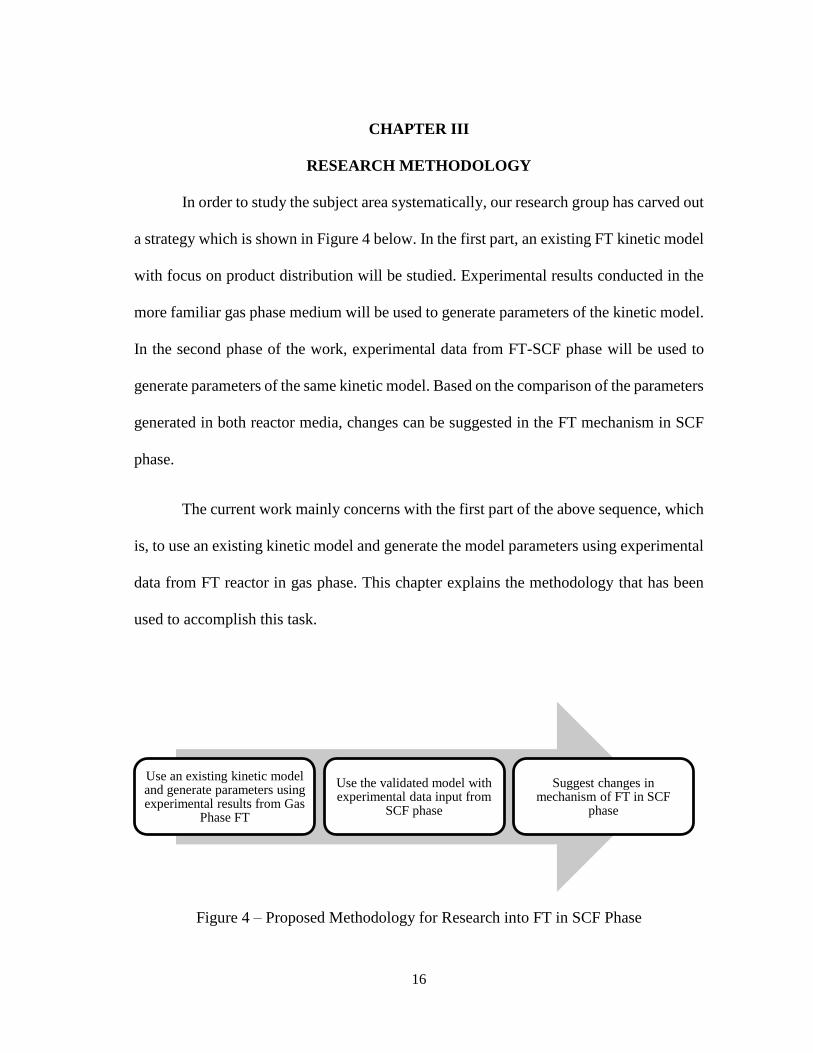
In order to study the subject area systematically, our research group has carved out

a strategy which is shown in Figure 4 below. In the first part, an existing FT kinetic model

with focus on product distribution will be studied. Experimental results conducted in the

more familiar gas phase medium will be used to generate parameters of the kinetic model.

In the second phase of the work, experimental data from FT-SCF phase will be used to

generate parameters of the same kinetic model. Based on the comparison of the parameters

generated in both reactor media, changes can be suggested in the FT mechanism in SCF

phase.

The current work mainly concerns with the first part of the above sequence, which

is, to use an existing kinetic model and generate the model parameters using experimental

data from FT reactor in gas phase. This chapter explains the methodology that has been

used to accomplish this task.

Figure 4 – Proposed Methodology for Research into FT in SCF Phase

Use an existing kinetic model and generate parameters using experimental results from Gas

Phase FT

Use the validated model with experimental data input from

SCF phase

Suggest changes in mechanism of FT in SCF

phase

17

3.1 Development of a kinetic model with focus on product distribution

Todic et al. [39] developed a comprehensive micro-kinetic model based on carbide

mechanism that predicts FT product distribution over a cobalt-based catalyst up to carbon

number 15. This model explains the non-ASF product distribution using a carbon number

dependent olefin formation rate (enc term, see Eq. 2, 4 below). Constant c is related to

weak Van der Waals interaction (c=-ΔE/RT) where ΔE is the contribution in the increase

of desorption energy per every CH2 group [39]. The rate equations for the olefins and

paraffins used in the model are listed below (Eq. 1-4).

rCH4= k5mK7

0.5PH2

1.5α1[S] (1)

rC2H4= k6ee2c√K7PH2

α1α2[S] (2)

rCnH2n+2= k5K7

0.5PH2

1.5α1α2 ∏ αi

n

i=3

[S] (3)

rCnH2n= k6enc√K7PH2

α1α2 ∏ αi

n

i=3

[S] (4)

These rate equations are obtained after writing up all the individual rate

expressions at each mechanistic step and working up the algebra involved. The reaction

steps that lead to these rate equations is listed in Table 1 on the next page. The

mathematical derivation for the above equations is available in supplementary information

by Todic et al [39].

18

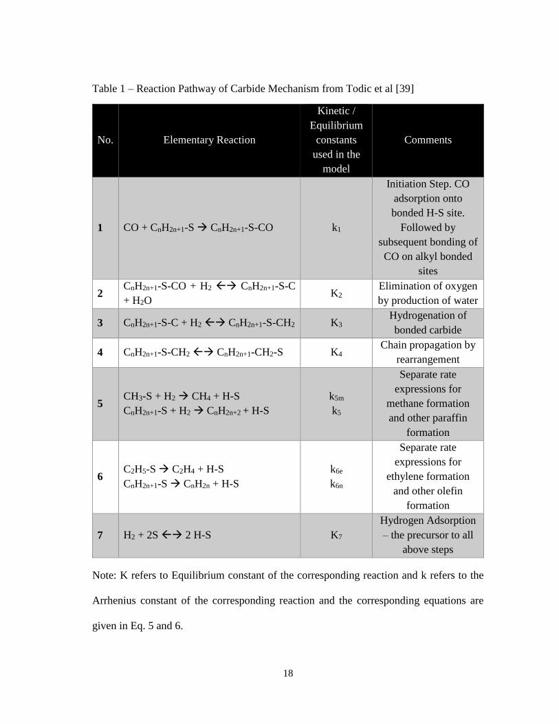
Table 1 – Reaction Pathway of Carbide Mechanism from Todic et al [39]

No. Elementary Reaction

Kinetic /

Equilibrium

constants

used in the

model

Comments

1 CO + CnH2n+1-S CnH2n+1-S-CO k1

Initiation Step. CO

adsorption onto

bonded H-S site.

Followed by

subsequent bonding of

CO on alkyl bonded

sites

2 CnH2n+1-S-CO + H2 CnH2n+1-S-C

+ H2O K2

Elimination of oxygen

by production of water

3 CnH2n+1-S-C + H2 CnH2n+1-S-CH2 K3 Hydrogenation of

bonded carbide

4 CnH2n+1-S-CH2 CnH2n+1-CH2-S K4 Chain propagation by

rearrangement

5 CH3-S + H2 CH4 + H-S

CnH2n+1-S + H2 CnH2n+2 + H-S

k5m

k5

Separate rate

expressions for

methane formation

and other paraffin

formation

6 C2H5-S C2H4 + H-S

CnH2n+1-S CnH2n + H-S

k6e

k6n

Separate rate

expressions for

ethylene formation

and other olefin

formation

7 H2 + 2S 2 H-S K7

Hydrogen Adsorption

– the precursor to all

above steps

Note: K refers to Equilibrium constant of the corresponding reaction and k refers to the

Arrhenius constant of the corresponding reaction and the corresponding equations are

given in Eq. 5 and 6.

19

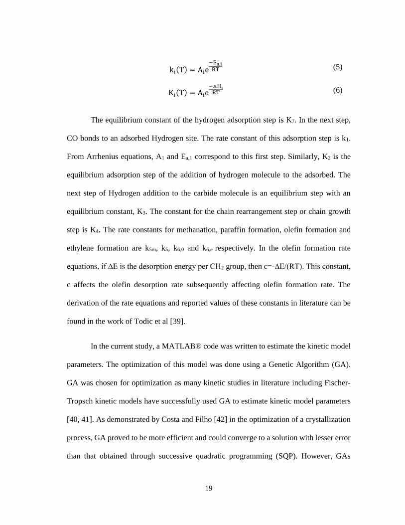
ki(T) = Aie−Ea,i

RT (5)

Ki(T) = Aie−△Hi

RT (6)

The equilibrium constant of the hydrogen adsorption step is K7. In the next step,

CO bonds to an adsorbed Hydrogen site. The rate constant of this adsorption step is k1.

From Arrhenius equations, A1 and Ea,1 correspond to this first step. Similarly, K2 is the

equilibrium adsorption step of the addition of hydrogen molecule to the adsorbed. The

next step of Hydrogen addition to the carbide molecule is an equilibrium step with an

equilibrium constant, K3. The constant for the chain rearrangement step or chain growth

step is K4. The rate constants for methanation, paraffin formation, olefin formation and

ethylene formation are k5m, k5, k6,0 and k6,e respectively. In the olefin formation rate

equations, if ∆E is the desorption energy per CH2 group, then c=-∆E/(RT). This constant,

c affects the olefin desorption rate subsequently affecting olefin formation rate. The

derivation of the rate equations and reported values of these constants in literature can be

found in the work of Todic et al [39].

In the current study, a MATLAB® code was written to estimate the kinetic model

parameters. The optimization of this model was done using a Genetic Algorithm (GA).

GA was chosen for optimization as many kinetic studies in literature including Fischer-

Tropsch kinetic models have successfully used GA to estimate kinetic model parameters

[40, 41]. As demonstrated by Costa and Filho [42] in the optimization of a crystallization

process, GA proved to be more efficient and could converge to a solution with lesser error

than that obtained through successive quadratic programming (SQP). However, GAs

20

suffer from the problem that they are time consuming which restricts their utility in real

time applications. Kinetic modeling is a one-time process and hence this is not a restriction

applicable to this study.

Chang et al [40] used GA to estimate unknown kinetic parameters of an FT kinetic

model derived from Langmuir-Hinshelwood-Hougen-Watson approach. Park and

Froment [41] demonstrated the use of GA to access the global minimum and showed that

low crossover probability with relatively high mutation probability was needed for a good

performance of GA. In both these studies, Levenberg-Marquardt (LM) optimizer was used

which takes GA results as initial values and performs further optimization. However, LM

optimization has not been performed in this current study as it is an add-on optimization

that can be added to the existing GA code to make a hybrid optimization tool.

One of the limitations of GA is that they are inefficient with constrained problems

[43]. Since the optimization of the current kinetic model does not involve constraints, this

was not a problem. No constraints were considered as essentially, genetic algorithms do

not need an initial guess to start the optimization. However, a range for each parameter

was supplied to the Genetic Algorithm to speed up optimization. It was found that without

the range, the optimization becomes very time consuming. These ranges for each

parameter were taken from literature [39].

21

Table 2 – Input Range for Model Parameters [39]

Parameter Description Range supplied to GA

A1 – A7, A5m, A6e A (Pre-exponential factor

in kinetic rate expression) 10-20 to 1020

ΔE1 Activation Energy of

Initiation step 50 kJ/mol to 150 kJ/mol

ΔE5, ΔE5m

Activation Energy of

Methane and Paraffin

formation step

70 kJ/mol to 120 kJ/mol

ΔE6, ΔE6e

Activation Energy of

Ethylene and Olefin

formation step

80 kJ/mol to 150 kJ/mol

ΔH2, ΔH3, ΔH4

Heat of reaction of water

formation step, carbide

hydrogenation step and

chain propagation by

rearrangement step

-50 kJ/mol to 50 kJ/mol

ΔH7 Heat of Adsorption of

hydrogen on vacant site

-100 kJ/mol to -10

kJ/mol

ΔE

Incremental increase in

desorption energy per

CH2 molecule

0 kJ/mol CH2 to 10

kJ/mol CH2

3.1.1 Genetic Algorithm

Genetic algorithm is an optimization technique that is based on the theory of

evolution. The concept is based on the idea that a better solution can be obtained if we

somehow combine good parts of the solution set and eliminate the poor parts of the

solution set, the same way nature does by combining the DNA of living organisms.

Genetic algorithms have been used to solve various engineering problems [44] as well as

for parameter estimation of kinetic models [41]. A dedicated toolbox is also available in

MATLAB® for genetic algorithm which provides an easy user interface to perform

optimization.

22

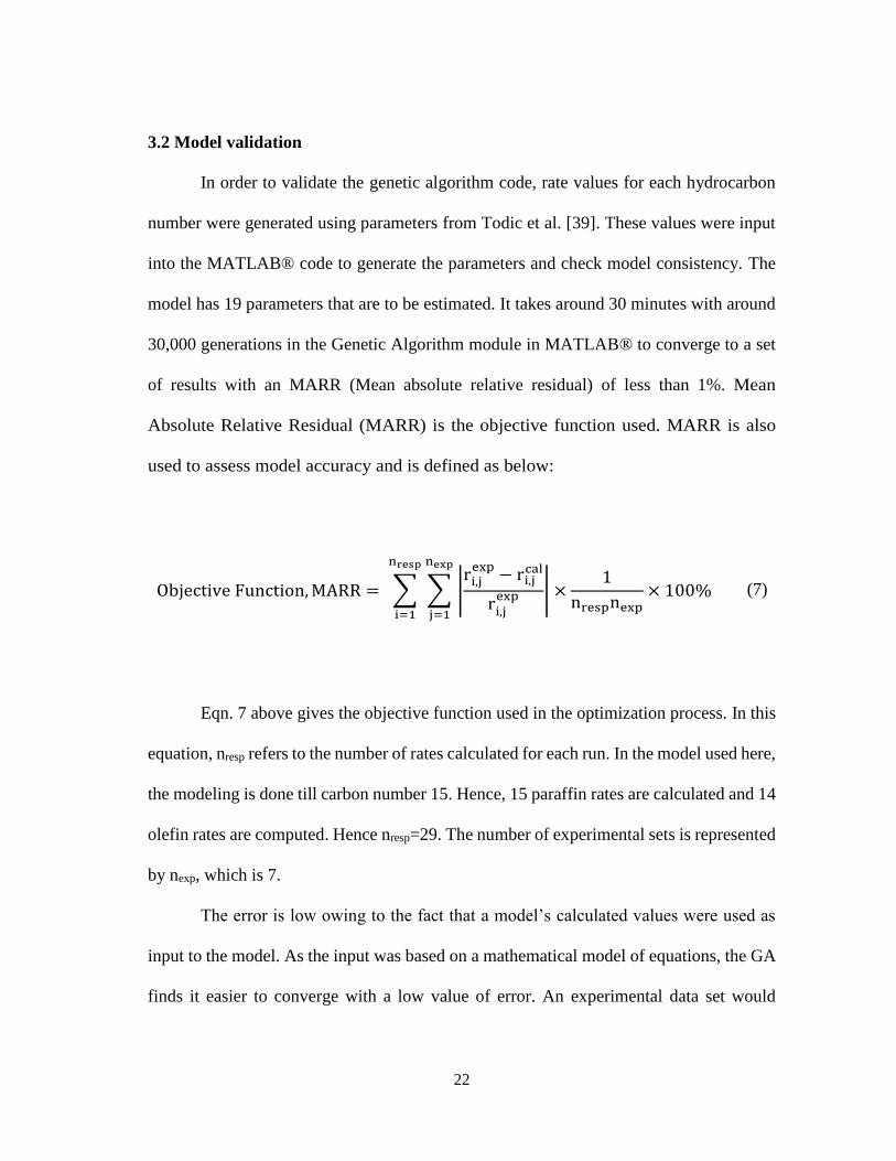
3.2 Model validation

In order to validate the genetic algorithm code, rate values for each hydrocarbon

number were generated using parameters from Todic et al. [39]. These values were input

into the MATLAB® code to generate the parameters and check model consistency. The

model has 19 parameters that are to be estimated. It takes around 30 minutes with around

30,000 generations in the Genetic Algorithm module in MATLAB® to converge to a set

of results with an MARR (Mean absolute relative residual) of less than 1%. Mean

Absolute Relative Residual (MARR) is the objective function used. MARR is also

used to assess model accuracy and is defined as below:

Objective Function, MARR = ∑ ∑ |ri,j

exp− ri,j

cal

ri,jexp | ×

1

nrespnexp× 100%

nexp

j=1

nresp

i=1

(7)

Eqn. 7 above gives the objective function used in the optimization process. In this

equation, nresp refers to the number of rates calculated for each run. In the model used here,

the modeling is done till carbon number 15. Hence, 15 paraffin rates are calculated and 14

olefin rates are computed. Hence nresp=29. The number of experimental sets is represented

by nexp, which is 7.

The error is low owing to the fact that a model’s calculated values were used as

input to the model. As the input was based on a mathematical model of equations, the GA

finds it easier to converge with a low value of error. An experimental data set would

23

consist of errors due to experimental uncertainties resulting in a higher % error. A

comparison of the model parameters used to calculate the rate values and the values

generated by the MATLAB® code is shown in Table 3.

Table 3 – Comparison of GA Results with Parameters determined by Todic et al [39]

Parameter Units

Estimated Value from Genetic

Algorithm

Value obtained by

Todic et al [39]

A1 mol/gcat/h/MPa 1.82E+06 1.83E+10

A2 - 620.59 5.8

A3 MPa-1 15.73 24.4

A4 - 995.89 2.9

A5 mol/gcat/h/MPa 2.58E+05 4.49E+05

A5,m mol/gcat/h/MPa 7.89E+06 8.43E+05

A6,0 mol/gcat/h 6.33E+07 7.47E+08

A6,e mol/gcat/h 1.86E+06 7.03E+08

A7 MPa-1 9.08E+07 1.00E-03

E1 kJ/mol 66.66 100.4

E5 kJ/mol 74.22 72.4

E5.m kJ/mol 76.31 63

E6,0 kJ/mol 91.09 97.2

E6,e kJ/mol 88.51 108.8

24

Table 3 (Continued)

∆H2 kJ/mol 26.54 8.68

∆H3 kJ/mol 15.09 9.44

∆H4 kJ/mol 21.23 7.9

∆H7 kJ/mol -10.09 -25

∆E kJ/mol/CH2 1.13 1.12

The heats of adsorption and the activation energies generated are physically

meaningful. However a closer look at the comparison of parameters reveals a large

difference in A7, the pre-exponential factor of the hydrogen adsorption step. The large

variation in the value of A7 can be attributed to the nature of the mathematical model

equations. The Genetic Algorithm aims to minimize the objective function which is the

normalization of the difference between the experimental and the calculated values of the

rate equation. As shown in Eqns. 1-4, 6 and 8, the term K7 (=A7*exp(-Ea/RT)) appears in

both the numerator and denominator of the hydrocarbon rate expressions. So, the

sensitivity of term is minimized irrespective of the value of A7 which could cause the large

difference of its reported value in this study and the one reported by Todic et al [39].

[S] =1

1 + √K7PH2+ √K7PH2

× (1 +1

K4+

1K3K4PH2

+PH2O

K2K3K4PH2

2 ) × (α1 + α1α2 + α1α2 × ∑ ∏ αjij=3

ni=3 )

(8)

25

The input rate values are compared with rates estimated by the model and are

plotted as shown in Figure 5. This validation step helps in testing the performance of the

Genetic Algorithm code written and number of generations required to attain a satisfactory

solution. It may be noted here that the purpose of this validation check step is to ascertain

the mathematical performance of the model with regards to fitting. This step helped to

identify errors in the code and fine tune the model based on the equations. Therefore, a

sensitivity analysis was not performed for each individual parameter.

Figure 5 – Validation of Genetic Algorithm Code

3.3 Experimental setup

The laboratory scale Fischer-Tropsch reactor designed and commissioned at Texas

A&M at Qatar is currently been used as an important part of the multi-scale investigation

on the performance of FT reactors in near critical and supercritical regions. This unit has

26

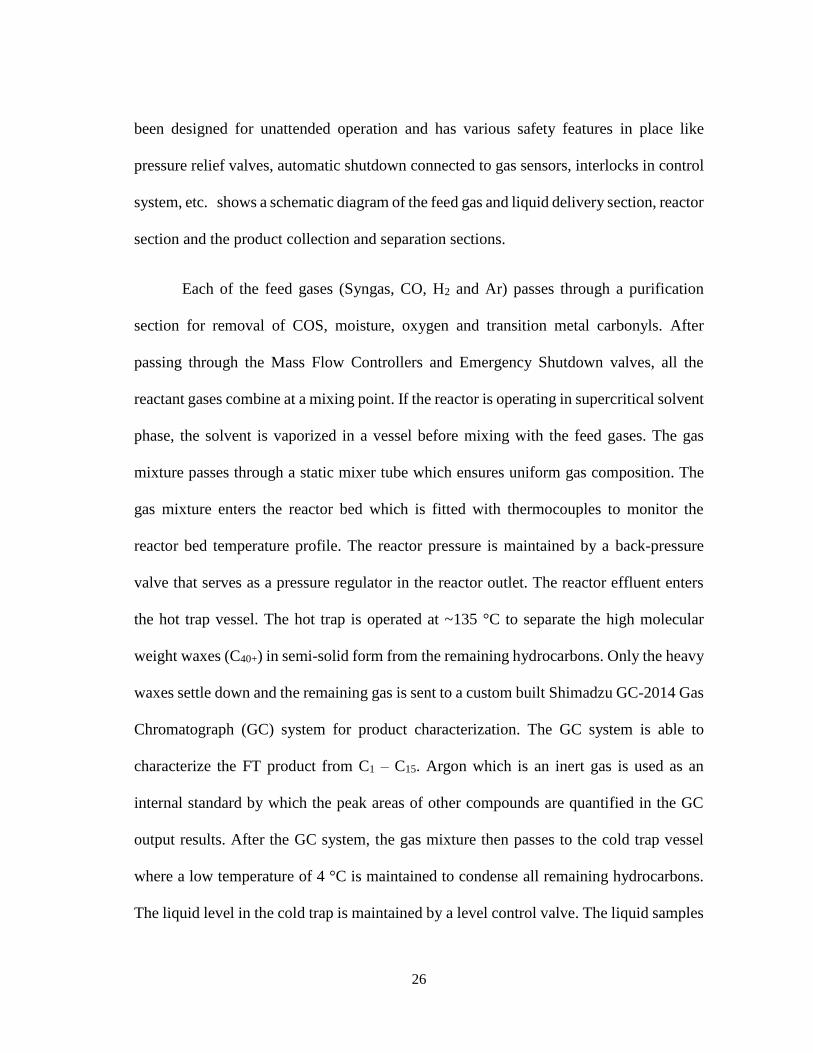
been designed for unattended operation and has various safety features in place like

pressure relief valves, automatic shutdown connected to gas sensors, interlocks in control

system, etc. shows a schematic diagram of the feed gas and liquid delivery section, reactor

section and the product collection and separation sections.

Each of the feed gases (Syngas, CO, H2 and Ar) passes through a purification

section for removal of COS, moisture, oxygen and transition metal carbonyls. After

passing through the Mass Flow Controllers and Emergency Shutdown valves, all the

reactant gases combine at a mixing point. If the reactor is operating in supercritical solvent

phase, the solvent is vaporized in a vessel before mixing with the feed gases. The gas

mixture passes through a static mixer tube which ensures uniform gas composition. The

gas mixture enters the reactor bed which is fitted with thermocouples to monitor the

reactor bed temperature profile. The reactor pressure is maintained by a back-pressure

valve that serves as a pressure regulator in the reactor outlet. The reactor effluent enters

the hot trap vessel. The hot trap is operated at ~135 °C to separate the high molecular

weight waxes (C40+) in semi-solid form from the remaining hydrocarbons. Only the heavy

waxes settle down and the remaining gas is sent to a custom built Shimadzu GC-2014 Gas

Chromatograph (GC) system for product characterization. The GC system is able to

characterize the FT product from C1 – C15. Argon which is an inert gas is used as an

internal standard by which the peak areas of other compounds are quantified in the GC

output results. After the GC system, the gas mixture then passes to the cold trap vessel

where a low temperature of 4 °C is maintained to condense all remaining hydrocarbons.

The liquid level in the cold trap is maintained by a level control valve. The liquid samples

27

are manually injected into a GC-MS system to further characterize higher hydrocarbons

up to carbon number 34. The individual sections are described in further detail in

subsequent sections.

28

Fig

ure

6 –

Blo

ck D

iagra

m o

f R

eact

or

29

3.3.1 Feed section

The feed section controls the flow rates of gases and liquids flowing into the FT

reactor. The gas feed consist of dedicated lines for hydrogen (H2), syngas (a mixture of

CO and H2), argon (Ar) and carbon monoxide (CO). A typical gas line starts at the gas

cylinder. Passing through the cylinder’s pressure regulator and flow restriction, the gas

enters the purification column. There is a provision for purge line, upstream of the

purification column to purge the lines during initial unit start-up. After purification, the

gas passes through a filter, an emergency shutdown valve (ESDV), forward pressure

regulator (PV), mass flow controller (MFC) and eventually enters the mixing point

through a non-return valve (NRV). A pressure relief valve (PSV) installed before the MFC

to prevent over pressurization of the system. The relief pressure is set at 135 bar. The feed

lines of all gases are similar except for CO where a pressure booster and a buffer vessel

are used to optimize CO usage. A part of the Ar is taken to the wax collector and the

Liquid product tank. This has been done to facilitate purging, when required. The Ar line

to Wax collector has been heat traced to increase wax temperature and enhance its mobility

and flow properties.

The solvent hexane feed system consists of solvent storage, purification column,

6-way valve, high-pressure HPLC pump and vaporization vessel. A plastic container

serves as the hexane tank. A N2 connection and a vent provision are provided to maintain

an inert atmosphere in the tank. The hexane from the tank flows through the purification

column into a 6-way valve port which serves to inject tracer chemicals into the system. A

HPLC pump transfers the hexane into a vaporizer column through NRV and a PSV. The

30

vaporizer heats and vaporizes the solvent feed before it mixes with the gaseous feed. The

combined gas + solvent feed enter a static mixer to ensure uniform mixing before the feed

enters the reactor. Starting from the vaporization vessel, all lines up to the cold trap are

heat insulated. A PSV is provided at the reactor inlet.

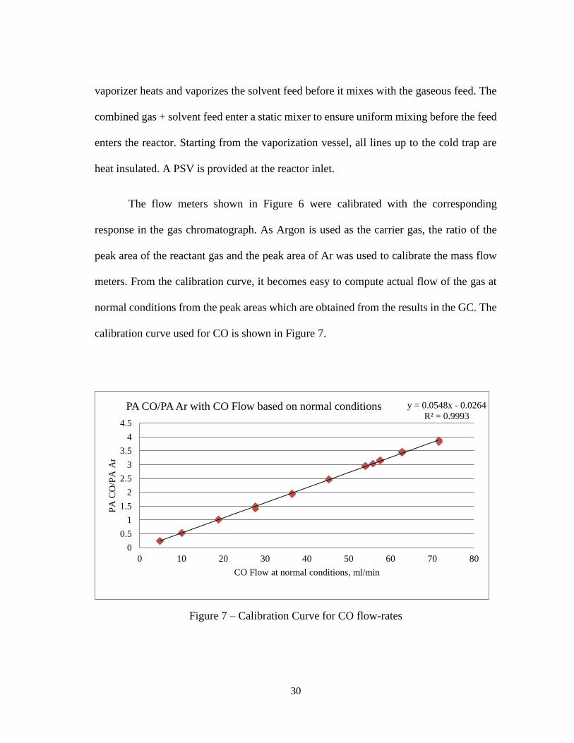
The flow meters shown in Figure 6 were calibrated with the corresponding

response in the gas chromatograph. As Argon is used as the carrier gas, the ratio of the

peak area of the reactant gas and the peak area of Ar was used to calibrate the mass flow

meters. From the calibration curve, it becomes easy to compute actual flow of the gas at

normal conditions from the peak areas which are obtained from the results in the GC. The

calibration curve used for CO is shown in Figure 7.

Figure 7 – Calibration Curve for CO flow-rates

y = 0.0548x - 0.0264

R² = 0.9993

0

0.5

1

1.5

2

2.5

3

3.5

4

4.5

0 10 20 30 40 50 60 70 80

PA

CO

/PA

Ar

CO Flow at normal conditions, ml/min

PA CO/PA Ar with CO Flow based on normal conditions

31

Apart from this, the mass flow-controllers of each reactant gas were calibrated

based on a counter installed in the vent of the cold trap. Every 5 mL of gas increase count

by 1 and this was displayed on the control screen on the computer. By varying the set point

of the flow-controller and calculating actual flow at standard conditions, 3 graphs were

plotted for the calibration of syngas, CO and H2 flow meters. This made calculations

simpler by directly converting set point to flow controller to actual standard flow rates of

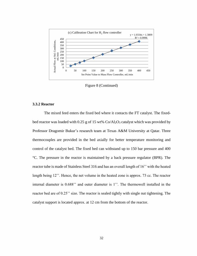
each individual gas. The calibration charts for the flow meters are shown below.

Figure 8 - Calibration Charts for CO, Syngas and H2 Flow Controllers

y = 1.1201x + 0.3057

R² = 0.9998

0

100

200

300

400

500

0 50 100 150 200 250 300 350 400 450Act

ual

Flo

w a

t S

td. C

on

dit

ion

s,

mL

/min

Set Point Value to Mass Flow Controller, mL/min

(a) Calibration Chart for CO flow controller

y = 1.0543x + 3.9237

R² = 0.9999

0

100

200

300

400

500

0 50 100 150 200 250 300 350 400 450

Act

ual

Flo

w a

t S

td. C

on

dit

ion

s,

mL

/min

Set Point Value to Mass Flow Controller, mL/min

(b) Calibration Chart for Syngas flow controller

32

Figure 8 (Continued)

3.3.2 Reactor

The mixed feed enters the fixed bed where it contacts the FT catalyst. The fixed-

bed reactor was loaded with 0.25 g of 15 wt% Co/Al2O3 catalyst which was provided by

Professor Dragomir Bukur’s research team at Texas A&M University at Qatar. Three

thermocouples are provided in the bed axially for better temperature monitoring and

control of the catalyst bed. The fixed bed can withstand up to 150 bar pressure and 400

°C. The pressure in the reactor is maintained by a back pressure regulator (BPR). The

reactor tube is made of Stainless Steel 316 and has an overall length of 16’’ with the heated

length being 12’’. Hence, the net volume in the heated zone is approx. 73 cc. The reactor

internal diameter is 0.688’’ and outer diameter is 1’’. The thermowell installed in the

reactor bed are of 0.25’’ size. The reactor is sealed tightly with single nut tightening. The

catalyst support is located approx. at 12 cm from the bottom of the reactor.

y = 1.0334x + 1.3809

R² = 0.9996

0

50

100

150

200

250

300

350

400

450

0 50 100 150 200 250 300 350 400 450

Act

ual

Flo

w a

t S

td. C

on

dit

ion

s,

mL

/min

Set Point Value to Mass Flow Controller, mL/min

(c) Calibration Chart for H2 flow controller

33

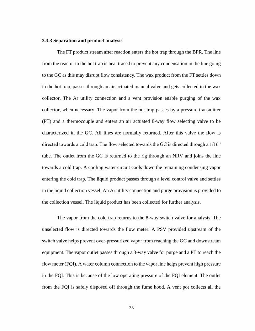
3.3.3 Separation and product analysis

The FT product stream after reaction enters the hot trap through the BPR. The line

from the reactor to the hot trap is heat traced to prevent any condensation in the line going

to the GC as this may disrupt flow consistency. The wax product from the FT settles down

in the hot trap, passes through an air-actuated manual valve and gets collected in the wax

collector. The Ar utility connection and a vent provision enable purging of the wax

collector, when necessary. The vapor from the hot trap passes by a pressure transmitter

(PT) and a thermocouple and enters an air actuated 8-way flow selecting valve to be

characterized in the GC. All lines are normally returned. After this valve the flow is

directed towards a cold trap. The flow selected towards the GC is directed through a 1/16”

tube. The outlet from the GC is returned to the rig through an NRV and joins the line

towards a cold trap. A cooling water circuit cools down the remaining condensing vapor

entering the cold trap. The liquid product passes through a level control valve and settles

in the liquid collection vessel. An Ar utility connection and purge provision is provided to

the collection vessel. The liquid product has been collected for further analysis.

The vapor from the cold trap returns to the 8-way switch valve for analysis. The

unselected flow is directed towards the flow meter. A PSV provided upstream of the

switch valve helps prevent over-pressurized vapor from reaching the GC and downstream

equipment. The vapor outlet passes through a 3-way valve for purge and a PT to reach the

flow meter (FQI). A water column connection to the vapor line helps prevent high pressure

in the FQI. This is because of the low operating pressure of the FQI element. The outlet

from the FQI is safely disposed off through the fume hood. A vent pot collects all the

34

liquid or vapor discharged through any relief valves. The vapor is disposed through the

fume hood and the liquid is drained at regular intervals.

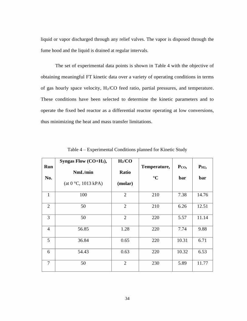
The set of experimental data points is shown in Table 4 with the objective of

obtaining meaningful FT kinetic data over a variety of operating conditions in terms

of gas hourly space velocity, H2/CO feed ratio, partial pressures, and temperature.

These conditions have been selected to determine the kinetic parameters and to

operate the fixed bed reactor as a differential reactor operating at low conversions,

thus minimizing the heat and mass transfer limitations.

Table 4 – Experimental Conditions planned for Kinetic Study

Run

No.

Syngas Flow (CO+H2),

NmL/min

(at 0 °C, 1013 kPA)

H2/CO

Ratio

(molar)

Temperature,

°C

PCO,

bar

PH2,

bar

1 100 2 210 7.38 14.76

2 50 2 210 6.26 12.51

3 50 2 220 5.57 11.14

4 56.85 1.28 220 7.74 9.88

5 36.84 0.65 220 10.31 6.71

6 54.43 0.63 220 10.32 6.53

7 50 2 230 5.89 11.77

35

3.4 Analysis of the product distribution

The product analysis from the custom built Shimadzu GC-2014 Gas

Chromatograph for each experimental run was done to identify hydrocarbon peaks. The

details on the calculations can be found in Appendix A. The gas chromatograph consists

of 3 separate channels – 2 TCD (Thermal Conductivity Detector) channels and 1 FID

(Flame Ionization Detector) channel. The first TCD column separates H2, Ar (carrier gas),

CO and CO2. The second TCD column exclusively contains the H2 peak. This was done

to improve the accuracy of H2 detection. The third channel which is the FID column is

capable of separating the hydrocarbon products from C1 up to C15. Table 5 and Table 6

give the details on the column and Figure 9 shows the column oven temperature program

used in the GC.

Table 5 – Details of Columns used in GC

Column Specification

TCD-1 (for CH4, CO) Rt-MS-5A 0.53 mm (ID), 30 m length

TCD-1 (for CO2, C2 compounds) Rt-Q PLOT 0.53 mm (ID), 30 m length

Fixed in second GC oven Rtx-1 0.53 mm (ID), 60 m length

TCD-2 (for H2) Rt-MS-5A 0.53 mm (ID), 30 m length

36

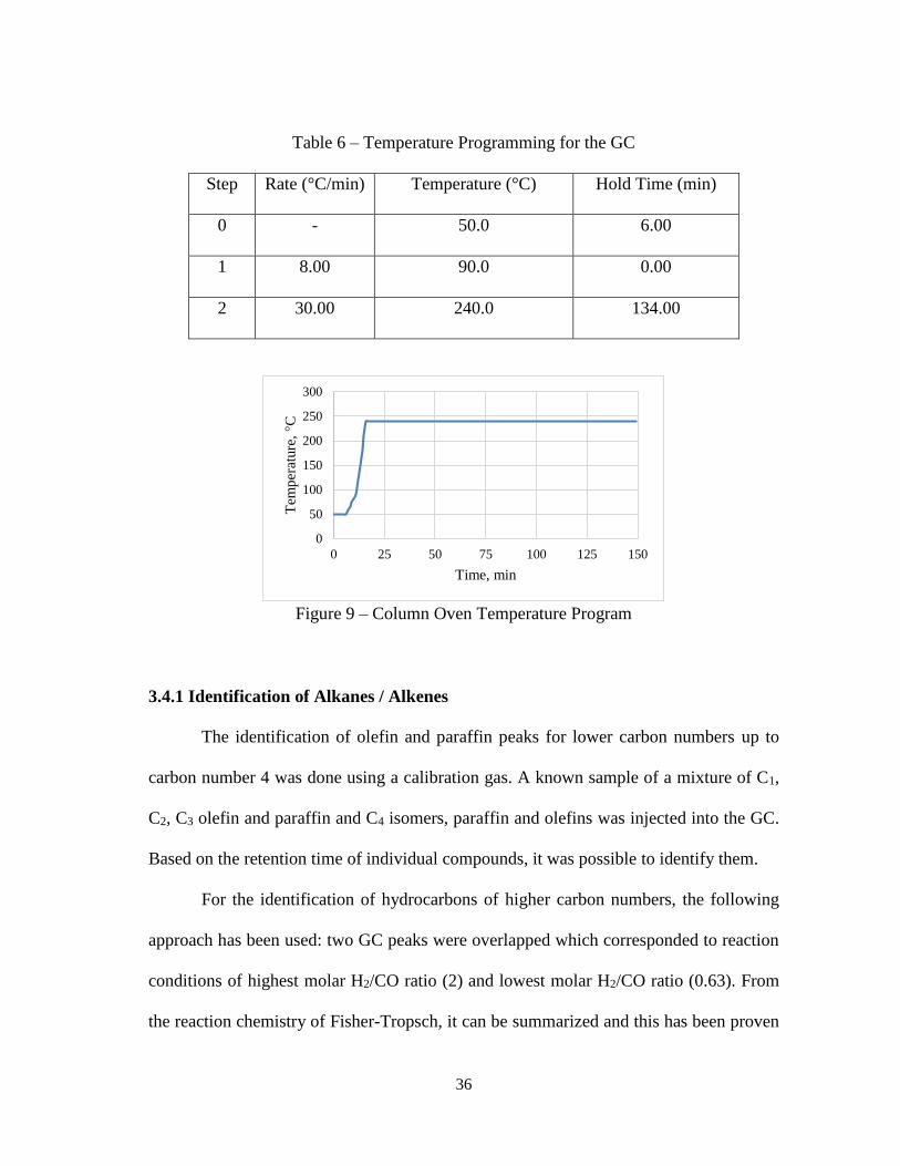
Table 6 – Temperature Programming for the GC

Step Rate (°C/min) Temperature (°C) Hold Time (min)

0 - 50.0 6.00

1 8.00 90.0 0.00

2 30.00 240.0 134.00

Figure 9 – Column Oven Temperature Program

3.4.1 Identification of Alkanes / Alkenes

The identification of olefin and paraffin peaks for lower carbon numbers up to

carbon number 4 was done using a calibration gas. A known sample of a mixture of C1,

C2, C3 olefin and paraffin and C4 isomers, paraffin and olefins was injected into the GC.

Based on the retention time of individual compounds, it was possible to identify them.

For the identification of hydrocarbons of higher carbon numbers, the following

approach has been used: two GC peaks were overlapped which corresponded to reaction

conditions of highest molar H2/CO ratio (2) and lowest molar H2/CO ratio (0.63). From

the reaction chemistry of Fisher-Tropsch, it can be summarized and this has been proven

0

50

100

150

200

250

300

0 25 50 75 100 125 150

Tem

per

ature

, °C

Time, min

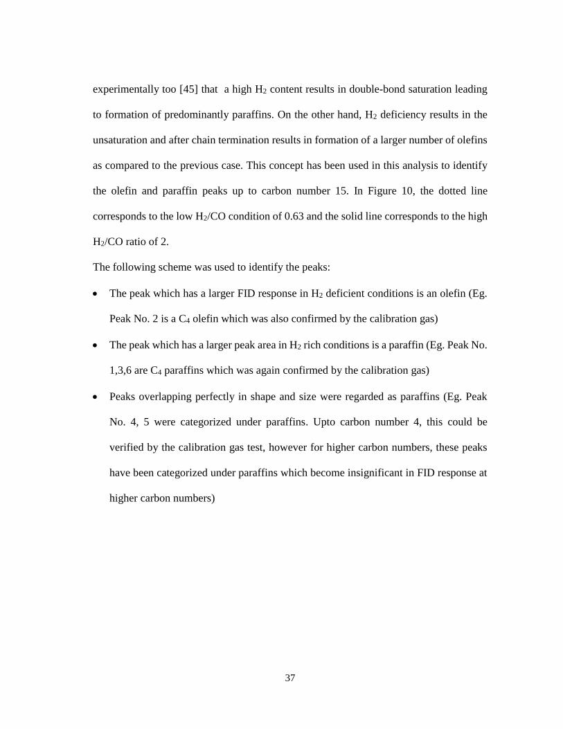
37

experimentally too [45] that a high H2 content results in double-bond saturation leading

to formation of predominantly paraffins. On the other hand, H2 deficiency results in the

unsaturation and after chain termination results in formation of a larger number of olefins

as compared to the previous case. This concept has been used in this analysis to identify

the olefin and paraffin peaks up to carbon number 15. In Figure 10, the dotted line

corresponds to the low H2/CO condition of 0.63 and the solid line corresponds to the high

H2/CO ratio of 2.

The following scheme was used to identify the peaks:

The peak which has a larger FID response in H2 deficient conditions is an olefin (Eg.

Peak No. 2 is a C4 olefin which was also confirmed by the calibration gas)

The peak which has a larger peak area in H2 rich conditions is a paraffin (Eg. Peak No.

1,3,6 are C4 paraffins which was again confirmed by the calibration gas)

Peaks overlapping perfectly in shape and size were regarded as paraffins (Eg. Peak

No. 4, 5 were categorized under paraffins. Upto carbon number 4, this could be

verified by the calibration gas test, however for higher carbon numbers, these peaks

have been categorized under paraffins which become insignificant in FID response at

higher carbon numbers)

38

Figure 10 – Identification of Olefin Peaks

3.4.2 Deconvolution of C3 peaks

Since the propylene and propane peaks have retention times close to each other,

they merge to form a composite curve as shown by the solid line in Figure 11. Hence, a

MATLAB code [46] was used for peak-splitting. The resultant peaks (dotted lines) were

normalized to the areas obtained and these values were used in the product distribution

analysis. The composite curve was resolved into 2 Gaussian peaks, the first one

corresponding to propylene and the next to propane. This is due to the fact that in the

calibration step it was observed from the GC response that up to carbon number 4, the

alkene always precedes the alkane.

0

5000

10000

15000

20000

25000

3 3.2 3.4 3.6 3.8 4 4.2 4.4

FID

Res

po

nse

Time, min

FID Response for low H2/CO ratio of 0.63

FID Response for high molar H2/CO ratio of 2

Peak 1-C4 paraffin

Peak 2-C4 olefin

Peak 3-C4 paraffin

Peak 4, 5-C4 paraffin

Peak 6-C4 paraffin

39

Time, min →

FID

Res

pon

se →

Figure 11 – Deconvolution of C3 peaks

40

CHAPTER IV

RESULTS AND DISCUSSION

This chapter discusses the experimental results obtained from the Reactor. The

experimental results are discussed first in Section 4.1. After working up the raw data

obtained from the reactor to the form required by the MATLAB program, the data was fed

to the MATLAB code to estimate parameters. This is discussed in detail in Section 4.2.

4.1 Experimental results

The reaction was carried out for a total time-on-stream (TOS) of 380 hours.

Sufficient time was allowed in each run for the unit to reach steady state which was

decided based on steady state behavior of CO conversion % graphs qualitatively. The

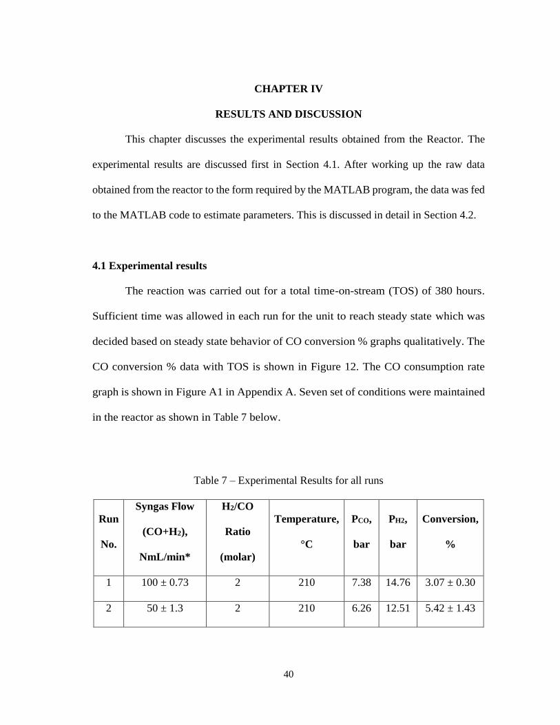
CO conversion % data with TOS is shown in Figure 12. The CO consumption rate

graph is shown in Figure A1 in Appendix A. Seven set of conditions were maintained

in the reactor as shown in Table 7 below.

Table 7 – Experimental Results for all runs

Run

No.

Syngas Flow

(CO+H2),

NmL/min*

H2/CO

Ratio

(molar)

Temperature,

°C

PCO,

bar

PH2,

bar

Conversion,

%

1 100 ± 0.73 2 210 7.38 14.76 3.07 ± 0.30

2 50 ± 1.3 2 210 6.26 12.51 5.42 ± 1.43

41

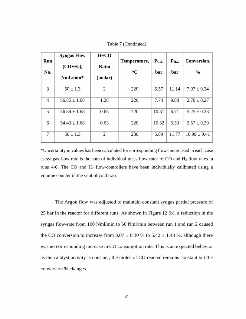
Table 7 (Continued)

Run

No.

Syngas Flow

(CO+H2),

NmL/min*

H2/CO

Ratio

(molar)

Temperature,

°C

PCO,

bar

PH2,

bar

Conversion,

%

3 50 ± 1.3 2 220 5.57 11.14 7.97 ± 0.24

4 56.85 ± 1.68 1.28 220 7.74 9.88 2.76 ± 0.27

5 36.84 ± 1.68 0.65 220 10.31 6.71 5.25 ± 0.28

6 54.43 ± 1.68 0.63 220 10.32 6.53 2.57 ± 0.29

7 50 ± 1.3 2 230 5.89 11.77 10.99 ± 0.41

*Uncertainty in values has been calculated for corresponding flow-meter used in each case

as syngas flow-rate is the sum of individual mass flow-rates of CO and H2 flow-rates in

runs 4-6. The CO and H2 flow-controllers have been individually calibrated using a

volume counter in the vent of cold trap.

The Argon flow was adjusted to maintain constant syngas partial pressure of

25 bar in the reactor for different runs. As shown in Figure 12 (b), a reduction in the

syngas flow-rate from 100 Nml/min to 50 Nml/min between run 1 and run 2 caused

the CO conversion to increase from 3.07 ± 0.30 % to 5.42 ± 1.43 %, although there

was no corresponding increase in CO consumption rate. This is an expected behavior

as the catalyst activity is constant, the moles of CO reacted remains constant but the

conversion % changes.

42

An increase in the reactor bed temperature by 10 °C (to 220 °C) in run 3 while

keeping the flow-rate constant, resulted in an increase in activity. Consequently, the

CO conversion rose to 7.97 ± 0.24 %. The conversion from the next run (run 4) was

lower due to the low H2/CO inlet ratio (i.e. lower partial pressure of H2). In run 5, the

syngas flow-rate was reduced and the H2/CO ratio was adjusted to 0.65. The

conversion and activity were found to increase due to lower flow-rates and higher

partial pressure of CO. In run 6, keeping the partial pressures of CO and H2 constant,

the syngas flowrate was increased from 36.84 to 54.43 Nml/min. This resulted in a

lower conversion and CO activity. Finally, the last run (run 7) was at 230 °C and hence

resulted in the highest CO activity among all runs. The CO conversion in all runs was

maintained at low levels, with all the runs being below 12%. This provided the meaningful

kinetic data required for input to the MATLAB® code.

43

Figure 12 – CO Conversion % with time-on-stream

Figure 13 – CO2 Selectivity with time-on-stream

1 2 3 4 5 6 7

0

5

10

15

20

25

0 50 100 150 200 250 300 350 400

CO

2S

elec

tivit

y

Time on Stream, hrs

CO2 Selectivity %

44

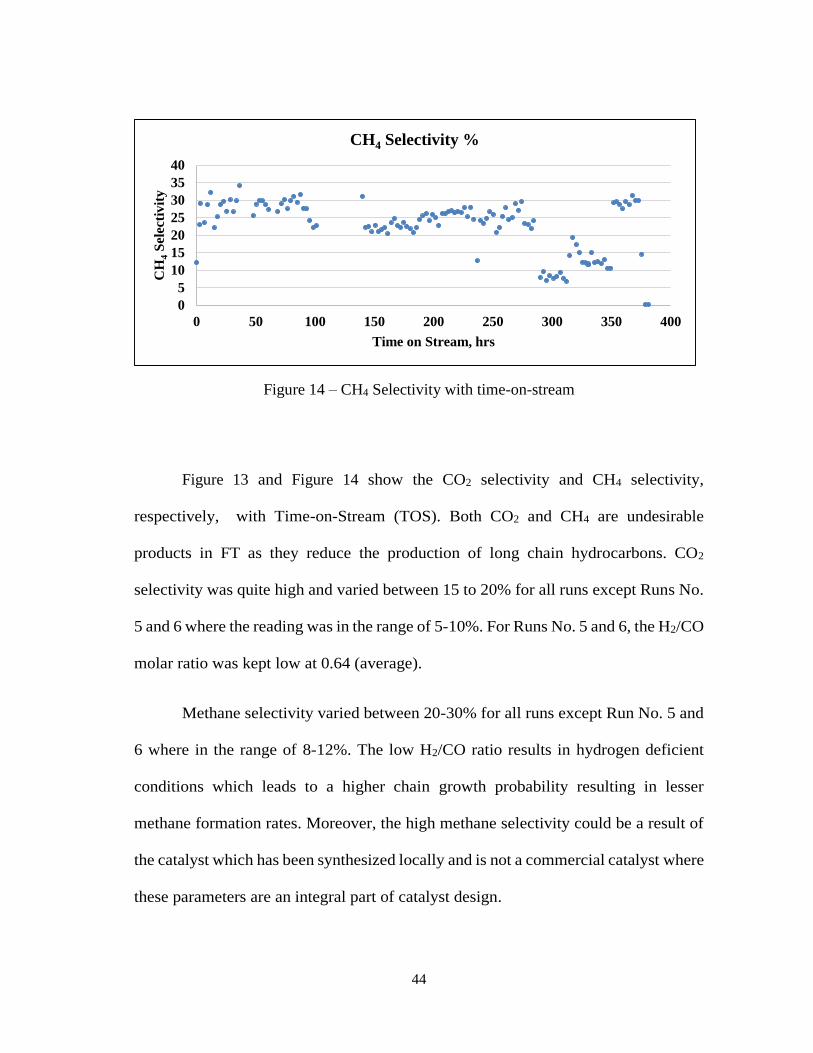
Figure 14 – CH4 Selectivity with time-on-stream

Figure 13 and Figure 14 show the CO2 selectivity and CH4 selectivity,

respectively, with Time-on-Stream (TOS). Both CO2 and CH4 are undesirable

products in FT as they reduce the production of long chain hydrocarbons. CO2

selectivity was quite high and varied between 15 to 20% for all runs except Runs No.

5 and 6 where the reading was in the range of 5-10%. For Runs No. 5 and 6, the H2/CO

molar ratio was kept low at 0.64 (average).

Methane selectivity varied between 20-30% for all runs except Run No. 5 and

6 where in the range of 8-12%. The low H2/CO ratio results in hydrogen deficient

conditions which leads to a higher chain growth probability resulting in lesser

methane formation rates. Moreover, the high methane selectivity could be a result of

the catalyst which has been synthesized locally and is not a commercial catalyst where

these parameters are an integral part of catalyst design.

0

5

10

15

20

25

30

35

40

0 50 100 150 200 250 300 350 400

CH

4S

elec

tiv

ity

Time on Stream, hrs

CH4 Selectivity %

45

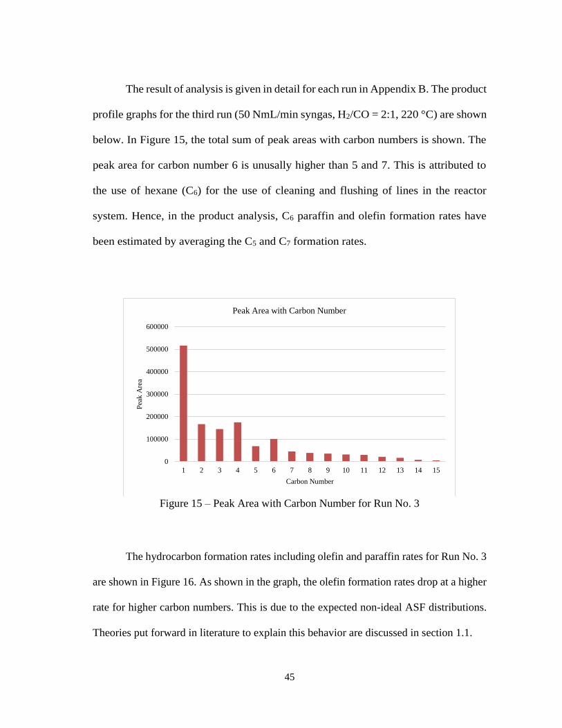
The result of analysis is given in detail for each run in Appendix B. The product

profile graphs for the third run (50 NmL/min syngas, H2/CO = 2:1, 220 °C) are shown

below. In Figure 15, the total sum of peak areas with carbon numbers is shown. The

peak area for carbon number 6 is unusally higher than 5 and 7. This is attributed to

the use of hexane (C6) for the use of cleaning and flushing of lines in the reactor

system. Hence, in the product analysis, C6 paraffin and olefin formation rates have

been estimated by averaging the C5 and C7 formation rates.

Figure 15 – Peak Area with Carbon Number for Run No. 3

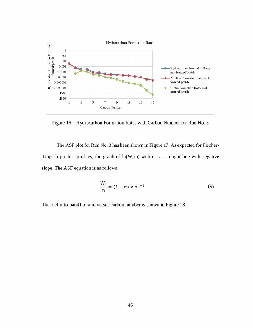
The hydrocarbon formation rates including olefin and paraffin rates for Run No. 3

are shown in Figure 16. As shown in the graph, the olefin formation rates drop at a higher

rate for higher carbon numbers. This is due to the expected non-ideal ASF distributions.

Theories put forward in literature to explain this behavior are discussed in section 1.1.

0

100000

200000

300000

400000

500000

600000

1 2 3 4 5 6 7 8 9 10 11 12 13 14 15

Pea

k A

rea

Carbon Number

Peak Area with Carbon Number

46

Figure 16 – Hydrocarbon Formation Rates with Carbon Number for Run No. 3

The ASF plot for Run No. 3 has been shown in Figure 17. As expected for Fischer-

Tropsch product profiles, the graph of ln(Wn/n) with n is a straight line with negative

slope. The ASF equation is as follows:

Wn

n= (1 − α) × αn−1 (9)

The olefin-to-paraffin ratio versus carbon number is shown in Figure 18.

1E-09

1E-08

0.0000001

0.000001

0.00001

0.0001

0.001

0.01

0.1

1

1 3 5 7 9 11 13 15

Hyd

roca

rbon

Form

atio

n R

ate,

mol

form

ed/g

cat/

h

Carbon Number

Hydrocarbon Formation Rates

Hydrocarbon Formation Rate,

mol formed/gcat/h

Paraffin Formation Rate, mol

formed/gcat/h

Olefin Formation Rate, mol

formed/gcat/h

47

Figure 17 – ASF Plot for Run No. 3

Figure 18 – Olefin-to-Paraffin Ratio with Carbon Number for Run No. 3

4.2 Model results

The data obtained from the reactor was fed into the GA program. The values for

the parameters obtained are given in Table 8. The convergence of the parameters has been

discussed in Appendix B.

y = -0.4293x - 1.8284

R² = 0.9413

-9

-8

-7

-6

-5

-4

-3

-2

-1

0

1 3 5 7 9 11 13 15

ln(W

n/n

)

Carbon Number

ASF Plot

0

0.1

0.2

0.3

0.4

0.5

0.6

0.7

0.8

0.9

1 3 5 7 9 11 13 15

Ole

fin

-to-P

araf

fin

Rat

io

Carbon Number

48

Table 8 – Model Results

Parameter Value Units

A1 1.87E+04 mol/gcat/h/MPa

A2 4.02E+04 -

A3 4.15E-03 MPa-1

A4 3.48E+01 -

A5 9.71E+05 mol/gcat/h/MPa

A5,m 1.55E+08 mol/gcat/h/MPa

A6,0 9.74E+09 mol/gcat/h

A6,e 6.47E+07 mol/gcat/h

A7 9.74E+09 MPa-1

E1 50.69 kJ/mol

E5 76.31 kJ/mol

E5.m 83.57 kJ/mol

E6,0 89.23 kJ/mol

E6,e 80.00 kJ/mol

∆H2 22.01 kJ/mol

∆H3 15.57 kJ/mol

∆H4 8.64 kJ/mol

∆H7 -16.70 kJ/mol

∆E 2.91 kJ/mol/CH2

49

The model parameters listed above are intrinsic constants. Hence, they are

expected to give a good fit of the experimental data and also satisfy physico-chemical

laws. The activation energies should be positive as they are expected to obey Arrhenius

temperature dependency. Heat of adsorption is always negative due to thermodynamic

nature of adsorption process. In the adsorption process, there is a loss of entropy as

molecules go from gaseous to an adsorbed phase. From the equation, ΔG=ΔH-TΔS, we

infer that when ΔS (entropy) is negative, ΔH (enthalpy change) should be negative to

give a negative value for ΔG (change in Gibbs free energy). The heat of hydrogen

adsorption, ΔH7 has a negative value of -16.7 kJ/mol similar to the reported value of -

15 kJ/mol for cobalt catalysts [47].

The activation energy for CO (E1) was estimated to be 50.69 kJ/mol, lower than

reported value of 80.7 kJ/mol by Pannell et al [48]. The paraffin formation activation

energy, E5 = 76.31 kJ/mol is comparable to the value of 74 kJ/mol reported by Chang et

al [40]. Activation energies for olefin formation rates (89.23 and 89 kJ/mol) are slightly

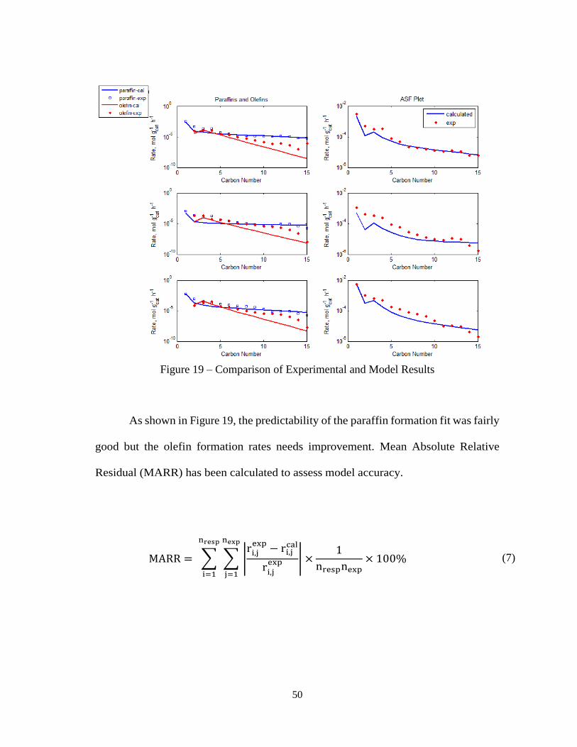
lower than those reported by Todic et al [39]. A comparison of the experimental and model

results for hydrocarbon formation rates and ASF plot is given in Figure 19.

50

Figure 19 – Comparison of Experimental and Model Results

As shown in Figure 19, the predictability of the paraffin formation fit was fairly

good but the olefin formation rates needs improvement. Mean Absolute Relative

Residual (MARR) has been calculated to assess model accuracy.

MARR = ∑ ∑ |ri,j

exp− ri,j

cal

ri,jexp | ×

1

nrespnexp× 100%

nexp

j=1

nresp

i=1

(7)

51

In the above equation, nresp refers to the number of rates calculated for each run. In

the model used here, the modeling is done till carbon number 15. Hence, 15 paraffin rates

are calculated and 14 olefin rates are computed. Hence nresp=29. The number of

experimental sets is represented by nexp, which is 7. The MARR for the model is

comparatively higher at 48.44%, than that reported by Todic et al (26.6%). The attribution

of this difference has been discussed in the section below.

4.2.1 Probable reasons for error

Though the model provides a reasonably good fit for paraffins, the error in

estimation of olefin formation rate is high. This discrepancy is attributed to two main

reasons as described below.

The genetic algorithm code used in the model estimates 19 parameters. Though

just one set of experimental data can also be used to obtain a solution set, the solution

set becomes more meaningful if the input data spans a wide range of input conditions.

In this study, 7 conditions have been used to generate the experimental data and each

condition gives 29 data points, which are hydrocarbon formation rates upto C15 of

both paraffins and olefins. Hence, the total number of data points for the entire

experiment is 203. More experiments planned could not be conducted due to logistical

reasons. The number of data points in the current experimental work is comparatively

lesser than the number of data points used by other researchers on models of similar

complexity. Todic et al [39] used 696 data points and Chang et al [40] used 504 data

points on similar kinetic models for prediction of FT product distribution.

52

Additionally, the number of experimental conditions is lesser than the number of

parameters (19). This could be one probable reason for the error in olefin prediction

rates.

Secondly, as described in Section 3.4.1, a methodology has been used to

identify olefins and paraffins in higher carbon number range. Though the technique is

based on engineering judgment and has a theoretical basis, ideally, the product

analysis should include a simultaneous MS (Mass Spectroscopy) and GC (Gas

Chromatograph) analysis. This might have resulted in missing some olefin peaks in

the higher carbon number range which might have led to the under-prediction of

olefins as shown in Figure 19.

Another source for experimental error could arise due to small sample loop

volume in the GC which means that too little was injected into the GC to “see” the

smaller peaks in the FID response. Experimental and simulation studies done by Gao

et al [49] suggest that one of the reasons for the deviations observed frequently in

experimental studies for higher hydrocarbon number product formation rates are due

to the inherent complex nature of product characterization of FT. They concluded that

maintaining low syngas conversion level, higher temperature and lower pressure of

hot trap could minimize this source of experimental error.

53

CHAPTER V

CONCLUSION & FUTURE WORK

This study represents a step forward towards the understanding of product

distribution in Fischer-Tropsch synthesis. As discussed in Chapter 3, this is a part of a

bigger research initiative that is aimed at understanding Fischer-Tropsch in non-

conventional reaction media like supercritical hydrocarbon solvents. A set of 7

experimental runs have been carried out and the experimental results have been input to a

carbide mechanism model in MATLAB to estimate the parameters in the model.

Considering the experimental results, it was observed that the hydrocarbon product

profile obtained was similar to the ones found in literature with high methane content and

decreasing yield of hydrocarbons with increasing carbon number. The main experimental

findings are listed below:

CO conversion % increased with increase in reactor bed temperature. This is an

expected behavior for exothermic reactions like FT due to temperature dependency in

Arrhenius rate equation and is also corroborated by experimental work carried out on

cobalt-based FT by Yao et al [50].

When the syngas flow-rate was reduced to half without changing the H2/CO ratio, the

CO conversion % increased but there was no change in CO conversion rate which

denotes that catalyst activity is constant. This observation has also been supported by

CFD simulations and experimental findings by Miroliaei et al [33].

54

CO2 selectivity was high and varied between 15% and 20% for most of the

experimental runs, except when the H2/CO ratio was low in which case it was 5-10%.

Methane selectivity had similar trend and it varied between 20-30% for all runs and in

the low H2/CO ratio runs, the selectivity was 8-12%. Hence both, the selectivity of

CH4 and CO2 dropped significantly at low H2/CO ratios.

As hexane was used for flushing the lines on the reactor system, C6 peak response was

abnormally high. The C6 formation rate was hence estimated by averaging out C5 and

C7 formation rates.

Summarizing the modeling results, the MARR (mean absolute relative residual)

for the fitted model is comparatively high at 48.44%. As evident from Figure 19, the

paraffin fit is better than olefin fit and this is attributed to the lesser number of data points

available for fitting and the probable mis-identification of some olefin peaks for higher

hydrocarbons. However, the model is able to predict the hydrocarbon formation rate trends

fairly well for cobalt catalyst based FT.

The next stage in this work is to carry out more experimental sets to overcome

some limitations of the current fitted model. This provides the necessary framework for

further studies of Fischer-Tropsch in supercritical hydrocarbon solvents. Data generated

experiments in the supercritical solvent phase will be compared with results from gas-

phase reaction which could give insight into the mechanism of FT in non-conventional

reaction media. The result of these studies could enable us to suggest modifications

55

in the existing model to account for the effect of the supercritical solvent on the

system.

This work will be linked with the research team’s effort to develop a master

FT reactor model that is suitable both for conventional (gas-phase) in non-

conventional (supercritical solvent) reaction media. Based on the outcome of these

studies, modifications to existing kinetic models can be suggested thereby accounting

for the effect of the supercritical solvent on the system. The overall goal will be to

model the whole reactor bed and optimize the supercritical FT process with a view to

potential scale-up and commercialization of this technology.

56

REFERENCES

[1] Tropsch, F.F.H., The synthesis of petroleum at atmospheric pressures from

gasification products of coal. Brennstoff-Chemie 1926. 17: p. 97-104.

[2] Elbashir, N.O., D.B. Bukur, E. Durham, and C.B. Roberts, Advancement of

Fischer-Tropsch synthesis via utilization of supercritical fluid reaction media.

AIChE J., 2010. 56: p. 997-1015.

[3] Savage, P.E., S. Gopalan, T.I. Mizan, C.J. Martino, and E.E. Brock, Reactions at

supercritical conditions: Applications and fundamentals. AIChE Journal, 1995.

41(7): p. 1723-1778.

[4] Yokota, K. and K. Fujimoto, Supercritical phase Fischer-Tropsch synthesis

reaction. Fuel, 1989. 68: p. 255-6.

[5] Huang, X. and C.B. Roberts, Selective Fischer-Tropsch synthesis over an Al2O3

supported cobalt catalyst in supercritical hexane. Fuel Process. Technol., 2003. 83:

p. 81-99.

[6] Bukur, D.B., X. Lang, A. Akgerman, and Z. Feng, Effect of process conditions on

olefin selectivity during conventional and supercritical Fischer-Tropsch synthesis.

Ind. Eng. Chem. Res., 1997. 36: p. 2580-2587.

[7] Li, X., X. Liu, Z.-W. Liu, K. Asami, and K. Fujimoto, Supercritical phase process

for direct synthesis of middle iso-paraffins from modified Fischer-Tropsch

reaction. Catal. Today, 2005. 106: p. 154-160.

57

[8] Liu, X., W. Linghu, X. Li, K. Asami, and K. Fujimoto, Effects of solvent on

Fischer–Tropsch synthesis. Applied Catalysis A: General, 2006. 303(2): p. 251-

257.

[9] Yokota, K. and K. Fujimoto, Supercritical-phase Fischer-Tropsch synthesis

reaction. 2. The effective diffusion of reactant and products in the supercritical-

phase reaction. Ind. Eng. Chem. Res., 1991. 30: p. 95-100.

[10] Huang, X., N.O. Elbashir, and C.B. Roberts, Supercritical Solvent Effects on

Hydrocarbon Product Distributions from Fischer-Tropsch Synthesis over an

Alumina-Supported Cobalt Catalyst. Ind. Eng. Chem. Res., 2004. 43: p. 6369-

6381.

[11] Tsubaki, N., K. Yoshii, and K. Fujimoto, Anti-ASF Distribution of Fischer-

Tropsch Hydrocarbons in Supercritical-Phase Reactions. J. Catal., 2002. 207: p.

371-375.

[12] Elbashir, N.O., Fundamentals and Design of the Supercritical Fluids Fischer

Tropsch. 2013: LAP LAMBERT Academic Publishing, Saarbrücken, Germany

[13] Rehan Hussain, J.H.B., Branislav Todic, Nimir O. Elbashir and Dragomir Bukur,

Development of Gas-to-Liquid Technologies from Micro- to Macro-scale,

Excellence and Impact of Research at Texas A&M University at Qatar. 2013.

[14] Bani Nasser, L.A., Simulation of Fischer-Tropsch Fixed-Bed Reactor in Different

Reaction Media, in Master of Science Thesis 2013. 2013, Texas A&M University

(available online).

58

[15] Flory, P.J., Molecular Size Distribution in Linear Condensation Polymers1.

Journal of the American Chemical Society, 1936. 58(10): p. 1877-1885.

[16] Puskas, I. and R.S. Hurlbut, Comments about the causes of deviations from the

Anderson–Schulz–Flory distribution of the Fischer–Tropsch reaction products.

Catalysis Today, 2003. 84(1–2): p. 99-109.

[17] Snel, R., Deviations of Fischer-Tropsch products from an Anderson-Schulz-Flory

distribution. Catalysis Letters, 1988. 1(10): p. 327-330.

[18] Elbashir, N.O. and C.B. Roberts, Enhanced Incorporation of α-Olefins in the

Fischer-Tropsch Synthesis Chain-Growth Process over an Alumina-Supported

Cobalt Catalyst in Near-Critical and Supercritical Hexane Media. Ind. Eng. Chem.

Res., 2005. 44: p. 505-521.

[19] Donnelly, T.J. and C.N. Satterfield, Product distributions of the Fischer-Tropsch

synthesis on precipitated iron catalysts. Applied Catalysis, 1989. 52(1): p. 93-114.

[20] Marvast, M.A., M. Sohrabi, S. Zarrinpashne, and G. Baghmisheh, Fischer-Tropsch

synthesis: Modeling and performance study for Fe-HZSM5 bifunctional catalyst.

Chemical Engineering & Technology, 2005. 28(1): p. 78-86.

[21] Liu, Q.S., Z.X. Zhang, and J.L. Zhou, Steady-state and dynamic behavior of fixed-

bed catalytic reactor for Fischer-Tropsch synthesis - II. Steady-state and dynamic

simulation results. Journal of Natural Gas Chemistry, 1999. 8(3): p. 238-247.

[22] Wang, Y.-N., Y.-Y. Xu, Y.-W. Li, Y.-L. Zhao, and B.-J. Zhang, Heterogeneous

modeling for fixed-bed Fischer–Tropsch synthesis: Reactor model and its

applications. Chemical Engineering Science, 2003. 58(3-6): p. 867-875.

59

[23] Guettel, R. and T. Turek, Comparison of different reactor types for low

temperature Fischer–Tropsch synthesis: A simulation study. Chemical

Engineering Science, 2009. 64(5): p. 955-964.

[24] Rahimpour, M.R., M.H. Khademi, and A.M. Bahmanpour, A comparison of

conventional and optimized thermally coupled reactors for Fischer–Tropsch

synthesis in GTL technology. Chemical Engineering Science, 2010. 65(23): p.

6206-6214.

[25] Moutsoglou, A. and P.P. Sunkara, Fischer–Tropsch Synthesis in a Fixed Bed

Reactor. Energy & Fuels, 2011. 25(5): p. 2242-2257.

[26] Brunner, K.M., J.C. Duncan, L.D. Harrison, K.E. Pratt, R.P.S. Peguin, C.H.

Bartholomew, and W.C. Hecker, A Trickle Fixed-Bed Recycle Reactor Model for

the Fischer-Tropsch Synthesis. International Journal of Chemical Reactor

Engineering, 2012. 10(1).

[27] Hooshyar, N., D. Vervloet, F. Kapteijn, P.J. Hamersma, R.F. Mudde, and J.R. van

Ommen, Intensifying the Fischer–Tropsch Synthesis by reactor structuring – A

model study. Chemical Engineering Journal, 2012. 207-208: p. 865-870.

[28] Jess, A. and C. Kern, Modeling of Multi-Tubular Reactors for Fischer-Tropsch

Synthesis. Chemical Engineering & Technology, 2009. 32(8): p. 1164-1175.

[29] Rafiq, M.H., H.A. Jakobsen, R. Schmid, and J.E. Hustad, Experimental studies and

modeling of a fixed bed reactor for Fischer–Tropsch synthesis using biosyngas.

Fuel Processing Technology, 2011. 92(5): p. 893-907.

60

[30] Sharma, A., R. Philippe, F. Luck, and D. Schweich, A simple and realistic fixed

bed model for investigating Fischer–Tropsch catalyst activity at lab-scale and

extrapolating to industrial conditions. Chemical Engineering Science, 2011.

66(24): p. 6358-6366.

[31] Lee, T.S. and J.N. Chung, Mathematical Modeling and Numerical Simulation of a

Fischer–Tropsch Packed Bed Reactor and Its Thermal Management for Liquid

Hydrocarbon Fuel Production using Biomass Syngas. Energy & Fuels, 2012.

26(2): p. 1363-1379.

[32] Pratt, J.W., A Fischer-Tropsch Synthesis Reactor Model Framework for Liquid

Biofuels Production, in SANDIA REPORT. 2012, Sandia National Laboratories.

[33] Miroliaei, A.R., F. Shahraki, H. Atashi, and R. Karimzadeh, Comparison of CFD

results and experimental data in a fixed bed Fischer–Tropsch synthesis reactor.

Journal of Industrial and Engineering Chemistry, 2012. 18(6): p. 1912-1920.

[34] Xia, B. and D.-W. Sun, Applications of computational fluid dynamics (cfd) in the

food industry: a review. Computers and Electronics in Agriculture, 2002. 34(1–

3): p. 5-24.

[35] P. Kaushal, S.H., Concept of Computational Fluid Dynamics (CFD) and its

Applications in Food Processing Equipment Design. Food Processing &

Technology, 2011. 3.

[36] Mogalicherla, A.K. and N.O. Elbashir, Development of a Kinetic Model for

Supercritical Fluids Fischer-Tropsch Synthesis. Energy & Fuels, 2011. 25(3): p.

878-889.

61

[37] Mogalicherla, A.K., E.E. Elmalik, and N.O. Elbashir, Enhancement in the

intraparticle diffusion in the supercritical phase Fischer–Tropsch synthesis.

Chemical Engineering and Processing: Process Intensification, 2012. 62: p. 59-

68.

[38] Elbashir, N.O.M., Utilization of supercritical fluids in the Fischer-Tropsch

synthesis over cobalt-based catalytic systems. 2004. p. 308 pp.

[39] Todic, B., T. Bhatelia, G.F. Froment, W. Ma, G. Jacobs, B.H. Davis, and D.B.

Bukur, Kinetic Model of Fischer–Tropsch Synthesis in a Slurry Reactor on Co–

Re/Al2O3Catalyst. Industrial & Engineering Chemistry Research, 2013. 52(2): p.

669-679.

[40] Chang, J., L. Bai, B. Teng, R. Zhang, J. Yang, Y. Xu, H. Xiang, and Y. Li, Kinetic

modeling of Fischer–Tropsch synthesis over catalyst in slurry phase reactor.

Chemical Engineering Science, 2007. 62(18–20): p. 4983-4991.

[41] Park, T.-Y. and G.F. Froment, A hybrid genetic algorithm for the estimation of

parameters in detailed kinetic models. Computers & Chemical Engineering, 1998.

22, Supplement 1(0): p. S103-S110.

[42] Costa, C.B.B. and R. Maciel Filho, Evaluation of optimisation techniques and

control variable formulations for a batch cooling crystallization process. Chemical

Engineering Science, 2005. 60(19): p. 5312-5322.

[43] Constrained minimization using GA. Available from:

http://www.mathworks.com/help/gads/constrained-minimization-using-ga.html.

62

[44] Silva, C.M. and E.C. Biscaia, Multi-Objective parameter estimation problems: an

improved strategy. Inverse Problems in Science and Engineering, 2004. 12(3): p.

297-316.

[45] Yates, I.C. and C.N. Satterfield, The hydrocarbon selectivity of cobalt Fischer-

Tropsch catalysts. 1991. p. Medium: X; Size: Pages: (38 p).

[46] O'Haver, T. http://www.mathworks.com/matlabcentral/fileexchange/23611-peak-

fitter. Available from:

http://www.mathworks.com/matlabcentral/fileexchange/23611-peak-fitter.

[47] Ojeda, M., R. Nabar, A.U. Nilekar, A. Ishikawa, M. Mavrikakis, and E. Iglesia,

CO activation pathways and the mechanism of Fischer–Tropsch synthesis. Journal

of Catalysis, 2010. 272(2): p. 287-297.

[48] Pannell, R.B., C.L. Kibby, and T.P. Kobylinski, A Steady-State Study of Fischer-

Tropsch Product Distributions Over Cobalt, Iron and Ruthenium, in Studies in

Surface Science and Catalysis. 1981. p. 447-459.

[49] Gao, J., B. Wu, L. Zhou, Y. Yang, X. Hao, J. Xu, Y. Xu, and Y. Li, Irregularities

in Product Distribution of Fischer–Tropsch Synthesis Due to Experimental

Artifact. Industrial & Engineering Chemistry Research, 2012. 51(36): p. 11618-

11628.

[50] Yao, Y., X. Liu, D. Hildebrandt, and D. Glasser, The effect of CO2 on a cobalt-

based catalyst for low temperature Fischer–Tropsch synthesis. Chemical

Engineering Journal, 2012. 193–194(0): p. 318-327.

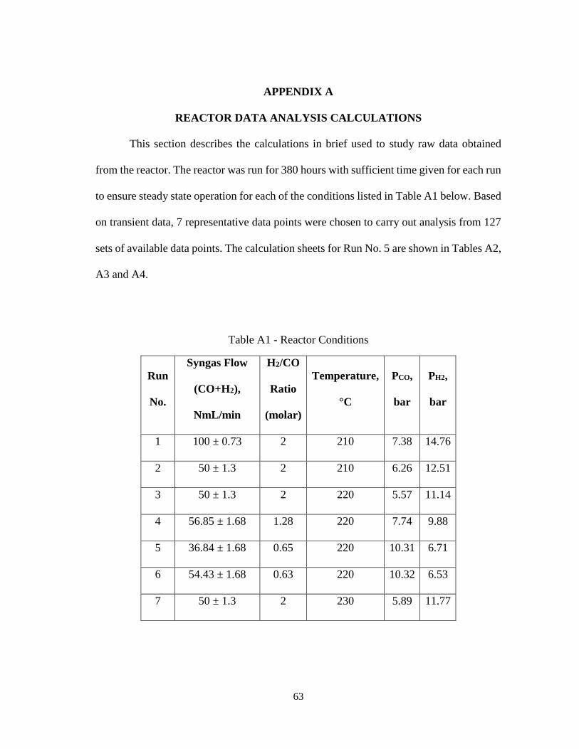
63

APPENDIX A

REACTOR DATA ANALYSIS CALCULATIONS

This section describes the calculations in brief used to study raw data obtained

from the reactor. The reactor was run for 380 hours with sufficient time given for each run

to ensure steady state operation for each of the conditions listed in Table A1 below. Based

on transient data, 7 representative data points were chosen to carry out analysis from 127

sets of available data points. The calculation sheets for Run No. 5 are shown in Tables A2,

A3 and A4.

Table A1 - Reactor Conditions

Run

No.

Syngas Flow

(CO+H2),

NmL/min

H2/CO

Ratio

(molar)

Temperature,

°C

PCO,

bar

PH2,

bar

1 100 ± 0.73 2 210 7.38 14.76

2 50 ± 1.3 2 210 6.26 12.51

3 50 ± 1.3 2 220 5.57 11.14

4 56.85 ± 1.68 1.28 220 7.74 9.88

5 36.84 ± 1.68 0.65 220 10.31 6.71

6 54.43 ± 1.68 0.63 220 10.32 6.53

7 50 ± 1.3 2 230 5.89 11.77

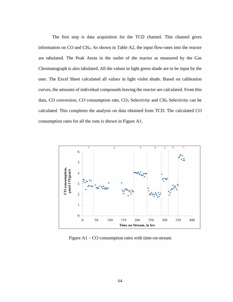
64

The first step is data acquisition for the TCD channel. This channel gives

information on CO and CH4. As shown in Table A2, the input flow-rates into the reactor

are tabulated. The Peak Areas in the outlet of the reactor as measured by the Gas

Chromatograph is also tabulated. All the values in light green shade are to be input by the

user. The Excel Sheet calculated all values in light violet shade. Based on calibration

curves, the amounts of individual compounds leaving the reactor are calculated. From this

data, CO conversion, CO consumption rate, CO2 Selectivity and CH4 Selectivity can be

calculated. This completes the analysis on data obtained from TCD. The calculated CO

consumption rates for all the runs is shown in Figure A1.

Figure A1 – CO consumption rates with time-on-stream

1 2 3 4 5 6 7

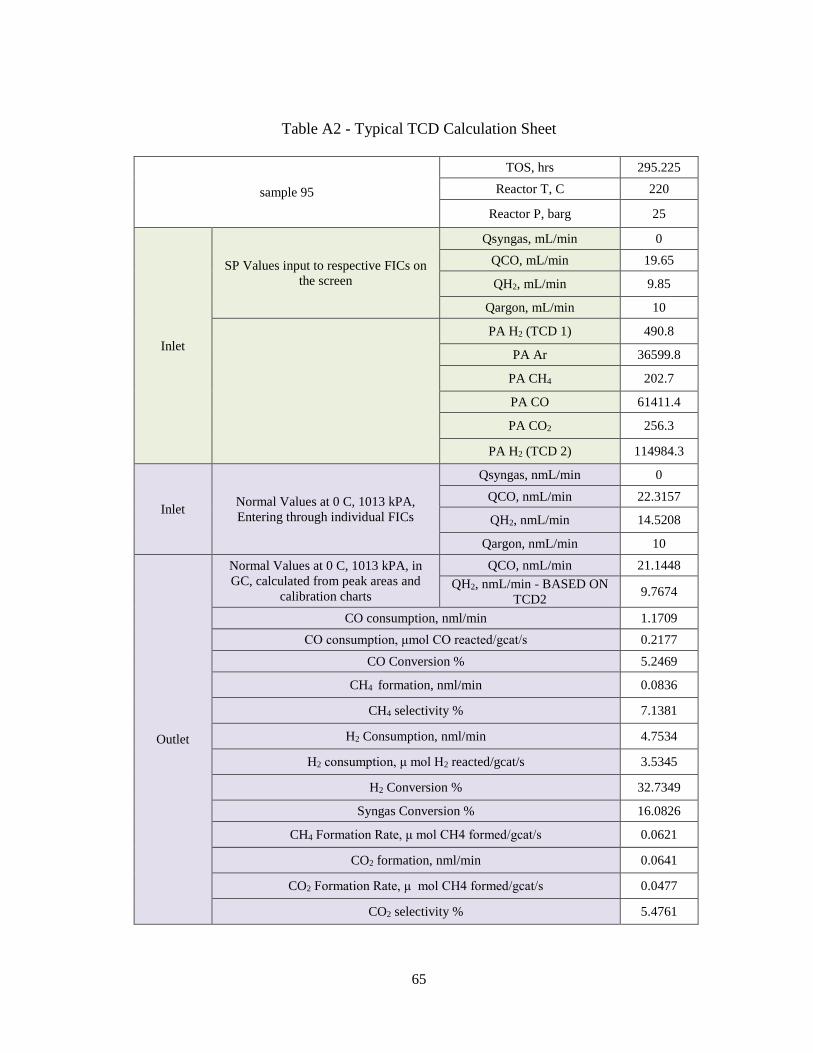
65

Table A2 - Typical TCD Calculation Sheet

sample 95

TOS, hrs 295.225

Reactor T, C 220

Reactor P, barg 25

Inlet

SP Values input to respective FICs on

the screen

Qsyngas, mL/min 0

QCO, mL/min 19.65

QH2, mL/min 9.85

Qargon, mL/min 10

PA H2 (TCD 1) 490.8

PA Ar 36599.8

PA CH4 202.7

PA CO 61411.4

PA CO2 256.3

PA H2 (TCD 2) 114984.3

Inlet Normal Values at 0 C, 1013 kPA,

Entering through individual FICs

Qsyngas, nmL/min 0

QCO, nmL/min 22.3157

QH2, nmL/min 14.5208

Qargon, nmL/min 10

Outlet

Normal Values at 0 C, 1013 kPA, in

GC, calculated from peak areas and

calibration charts

QCO, nmL/min 21.1448

QH2, nmL/min - BASED ON

TCD2 9.7674

CO consumption, nml/min 1.1709

CO consumption, μmol CO reacted/gcat/s 0.2177

CO Conversion % 5.2469

CH4 formation, nml/min 0.0836

CH4 selectivity % 7.1381

H2 Consumption, nml/min 4.7534

H2 consumption, μ mol H2 reacted/gcat/s 3.5345

H2 Conversion % 32.7349

Syngas Conversion % 16.0826

CH4 Formation Rate, μ mol CH4 formed/gcat/s 0.0621

CO2 formation, nml/min 0.0641

CO2 Formation Rate, μ mol CH4 formed/gcat/s 0.0477

CO2 selectivity % 5.4761

66

The FID channel gives information on the hydrocarbon products obtained from the

Fischer-Tropsch reaction. Table A3 shows the raw data obtained from the FID channel.

Based on the calibration gas test and the methodology explained in Section 3.4.1, the peaks

are identified as olefins or paraffins and listed in a tabular form. In the FID channel,

relative peak areas are proportional to weight fraction ratios. CH4 peak appears both in

TCD and the FID channel. Hence, the CH4 formation rate obtained from TCD channel is

used as a base to calculate other hydrocarbon formation rates. It may be noted here that

peak area ratios of 2 compounds in TCD channel are proportional to their molar fractions

and the peak area ratios obtained from FID channel are proportional to their weight

fractions. This concept has been used while calculating individual hydrocarbon formation

rates as shown in Table A4.

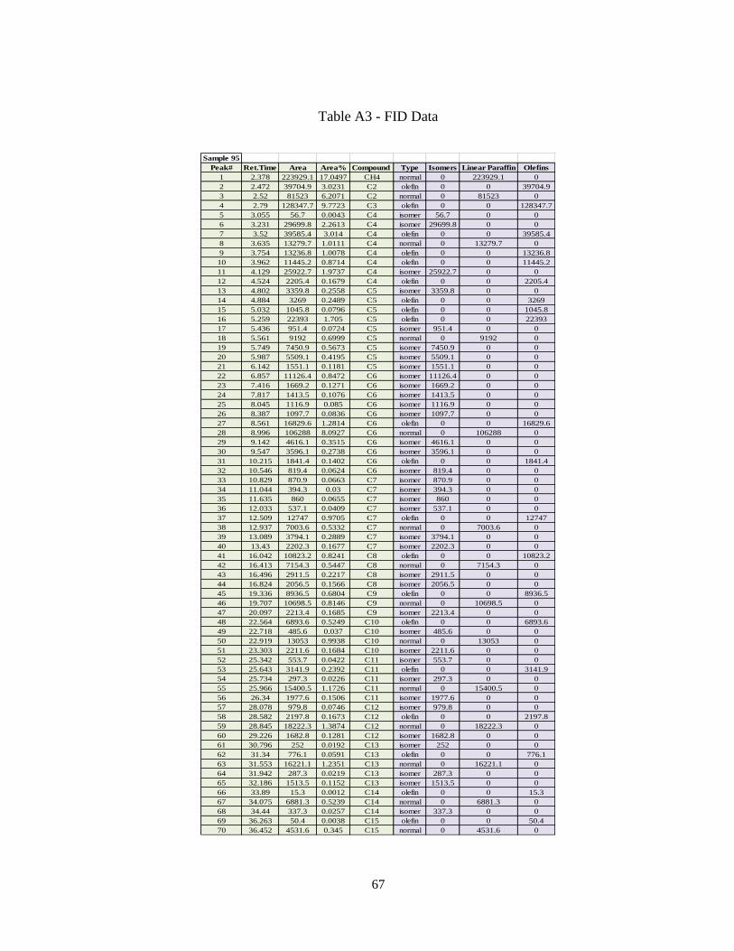
67

Table A3 - FID Data

Sample 95

Peak# Ret.Time Area Area% Compound Type Isomers Linear Paraffin Olefins

1 2.378 223929.1 17.0497 CH4 normal 0 223929.1 0

2 2.472 39704.9 3.0231 C2 olefin 0 0 39704.9

3 2.52 81523 6.2071 C2 normal 0 81523 0

4 2.79 128347.7 9.7723 C3 olefin 0 0 128347.7

5 3.055 56.7 0.0043 C4 isomer 56.7 0 0

6 3.231 29699.8 2.2613 C4 isomer 29699.8 0 0

7 3.52 39585.4 3.014 C4 olefin 0 0 39585.4

8 3.635 13279.7 1.0111 C4 normal 0 13279.7 0

9 3.754 13236.8 1.0078 C4 olefin 0 0 13236.8

10 3.962 11445.2 0.8714 C4 olefin 0 0 11445.2

11 4.129 25922.7 1.9737 C4 isomer 25922.7 0 0

12 4.524 2205.4 0.1679 C4 olefin 0 0 2205.4

13 4.802 3359.8 0.2558 C5 isomer 3359.8 0 0

14 4.884 3269 0.2489 C5 olefin 0 0 3269

15 5.032 1045.8 0.0796 C5 olefin 0 0 1045.8

16 5.259 22393 1.705 C5 olefin 0 0 22393

17 5.436 951.4 0.0724 C5 isomer 951.4 0 0

18 5.561 9192 0.6999 C5 normal 0 9192 0

19 5.749 7450.9 0.5673 C5 isomer 7450.9 0 0

20 5.987 5509.1 0.4195 C5 isomer 5509.1 0 0

21 6.142 1551.1 0.1181 C5 isomer 1551.1 0 0

22 6.857 11126.4 0.8472 C6 isomer 11126.4 0 0

23 7.416 1669.2 0.1271 C6 isomer 1669.2 0 0

24 7.817 1413.5 0.1076 C6 isomer 1413.5 0 0

25 8.045 1116.9 0.085 C6 isomer 1116.9 0 0

26 8.387 1097.7 0.0836 C6 isomer 1097.7 0 0

27 8.561 16829.6 1.2814 C6 olefin 0 0 16829.6

28 8.996 106288 8.0927 C6 normal 0 106288 0

29 9.142 4616.1 0.3515 C6 isomer 4616.1 0 0

30 9.547 3596.1 0.2738 C6 isomer 3596.1 0 0

31 10.215 1841.4 0.1402 C6 olefin 0 0 1841.4

32 10.546 819.4 0.0624 C6 isomer 819.4 0 0

33 10.829 870.9 0.0663 C7 isomer 870.9 0 0

34 11.044 394.3 0.03 C7 isomer 394.3 0 0

35 11.635 860 0.0655 C7 isomer 860 0 0

36 12.033 537.1 0.0409 C7 isomer 537.1 0 0

37 12.509 12747 0.9705 C7 olefin 0 0 12747

38 12.937 7003.6 0.5332 C7 normal 0 7003.6 0

39 13.089 3794.1 0.2889 C7 isomer 3794.1 0 0

40 13.43 2202.3 0.1677 C7 isomer 2202.3 0 0

41 16.042 10823.2 0.8241 C8 olefin 0 0 10823.2

42 16.413 7154.3 0.5447 C8 normal 0 7154.3 0

43 16.496 2911.5 0.2217 C8 isomer 2911.5 0 0

44 16.824 2056.5 0.1566 C8 isomer 2056.5 0 0

45 19.336 8936.5 0.6804 C9 olefin 0 0 8936.5

46 19.707 10698.5 0.8146 C9 normal 0 10698.5 0

47 20.097 2213.4 0.1685 C9 isomer 2213.4 0 0

48 22.564 6893.6 0.5249 C10 olefin 0 0 6893.6

49 22.718 485.6 0.037 C10 isomer 485.6 0 0

50 22.919 13053 0.9938 C10 normal 0 13053 0

51 23.303 2211.6 0.1684 C10 isomer 2211.6 0 0

52 25.342 553.7 0.0422 C11 isomer 553.7 0 0

53 25.643 3141.9 0.2392 C11 olefin 0 0 3141.9

54 25.734 297.3 0.0226 C11 isomer 297.3 0 0

55 25.966 15400.5 1.1726 C11 normal 0 15400.5 0

56 26.34 1977.6 0.1506 C11 isomer 1977.6 0 0

57 28.078 979.8 0.0746 C12 isomer 979.8 0 0

58 28.582 2197.8 0.1673 C12 olefin 0 0 2197.8

59 28.845 18222.3 1.3874 C12 normal 0 18222.3 0

60 29.226 1682.8 0.1281 C12 isomer 1682.8 0 0

61 30.796 252 0.0192 C13 isomer 252 0 0

62 31.34 776.1 0.0591 C13 olefin 0 0 776.1

63 31.553 16221.1 1.2351 C13 normal 0 16221.1 0

64 31.942 287.3 0.0219 C13 isomer 287.3 0 0

65 32.186 1513.5 0.1152 C13 isomer 1513.5 0 0

66 33.89 15.3 0.0012 C14 olefin 0 0 15.3

67 34.075 6881.3 0.5239 C14 normal 0 6881.3 0

68 34.44 337.3 0.0257 C14 isomer 337.3 0 0

69 36.263 50.4 0.0038 C15 olefin 0 0 50.4

70 36.452 4531.6 0.345 C15 normal 0 4531.6 0

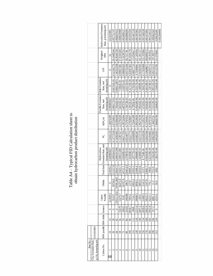
68

Tab

le A

4 –

Typic

al F

ID C

alcu

lati

on s

hee

t to

obta

in h

ydro

carb

on p

rod

uct

dis

trib

uti

on

CH

4 F

orm

atio

n R

ate,

g C

H4 form

ed/g

cat/h

0.0

1431883

Car

bon

No.

MW

par

affin

MW

ole

finIs

om

ers

Lin

ear

Par

affin

Ole

fins

Tota

l Sum

Hyd

roca

rbon

Form

atio

n R

ate,

mol

form

ed/g

cat/h

Wn

ln(W

n/n

)

Par

affin

Form

atio

n

Rat

e, m

ol

form

ed/g

cat/h

Ole

fin F

orm

atio

n

Rat

e, m

ol

form

ed/g

cat/h

O/P

Wei

ghte

d

MW

Hyd

roca

rbon

Form

atio

n

Rat

e, g

form

ed/g

cat/h

116

14

0223929.1

0223929.1

0.0

00894927

0.2

5442126

-1.3

6876389

0.0

00894927

00

16

0.0

1431883

230

28

081523

39704.9

121227.9

0.0

00264159

0.1

3773536

-2.6

7556831

0.0

00173762

9.0

6741E

-05

0.5

2182776

29.3

449544

0.0

07751747

344

42

053551.3

333

74796.3

667

128347.7

0.0

00191598

0.1

4582465

-3.0

2396268

7.7

8242E

-05

0.0

00113875

1.4

6323338

42.8

344728

0.0

08207012

458

56

55679

13279.7

66472.8

135431.7

0.0

00151881

0.1

5387327

-3.2

5792028

7.6

0255E

-05

7.5

902E

-05

0.9

9837481

57.0

183569

0.0

08659989

572

70

18822

9192

26707.8

54722.1

4.9

2669E

-05

0.0

6217354

-4.3

8726364

2.4

8797E

-05

2.4

397E

-05

0.9

8060205

71.0

238752

0.0

03499127

686

84

25455

106288

18671

150414.3

3.3

7987E

-05

0.0

5149777

-4.7

5797632

1.7

4473E

-05

1.6

3571E

-05

0.9

3751436

85.7

51739

0.0

02898295

7100

98

8658.7

7003.6

12747

28409.3

1.8

3304E

-05

0.0

3227776

-5.3

7928697

1.0

015E

-05

8.3

1723E

-06

0.8

3047463

99.1

026178

0.0

01816593

8114

112

4968

7154.3

10823.2

22945.5

1.2

9777E

-05

0.0

2606996

-5.7

2641308

6.7

995E

-06

6.1

7923E

-06

0.9

0877733

113.0

56617

0.0

01467218

9128

126

2213.4

10698.5

8936.5

21848.4

1.0

9848E

-05

0.0

2482347

-5.8

9319026

6.4

5026E

-06

4.5

3517E

-06

0.7

030994

127.1

81954

0.0

01397065

10

142

140

2697.2

13053

6893.6

22643.8

1.0

2406E

-05

0.0

2572718

-5.9

6279239

7.0

9242E

-06

3.1

4858E

-06

0.4

4393595

141.3

91127

0.0

01447926

11

156

154

2828.6

15400.5

3141.9

21371

8.7

764E

-06

0.0

2428106

-6.1

1595379

7.4

7201E

-06

1.3

0457E

-06

0.1

7459468

155.7

05966

0.0

01366538

12

170

168

2662.6

18222.3

2197.8

23082.7

8.6

9203E

-06

0.0

2622584

-6.1

2591661

7.8

5562E

-06

8.3

6519E

-07

0.1

0648671

169.8

09572

0.0

01475991

13

184

182

2052.8

16221.1

776.1

19050

6.6

2318E

-06

0.0

2164402

-6.3

9797563

6.3

5054E

-06

2.7

2674E

-07

0.0

4293712

183.9

1852

0.0

01218125

14

198

196

337.3

6881.3

15.3

7233.9

2.3

3622E

-06

0.0

0821893

-7.4

403724

2.3

3123E

-06

4.9

9151E

-09

0.0

0214115

197.9

9577

0.0

00462562

15

212

210

04531.6

50.4

4582

1.3

8217E

-06

0.0

0520593

-7.9

6600799

1.3

6682E

-06

1.5

3465E

-08

0.0

1122782

211.9

78001

0.0

0029299

0.0

56280006

Run

No. 5

69

APPENDIX B

CONVERGENCE OF GENETIC ALGORITHM RESULTS

As mentioned in chapter 3 on the research methodology followed, genetic algorithm is the

optimization tool used for estimating the parameters of the kinetic model. Unlike

traditional search algorithms, the GA does not search for solutions in the state space. GAs

work in solution space and build new, hopefully better solutions based on existing ones.

In the current optimization study, to ascertain the convergence of all 19 parameters to a

stable value, each parameter is plotted with generation and is shown in Figure B1. The

plot was made for 50,000 generations and an f-count of 1,000,000. As is evident, the

population stabilizes with time and converges to a concordant value.

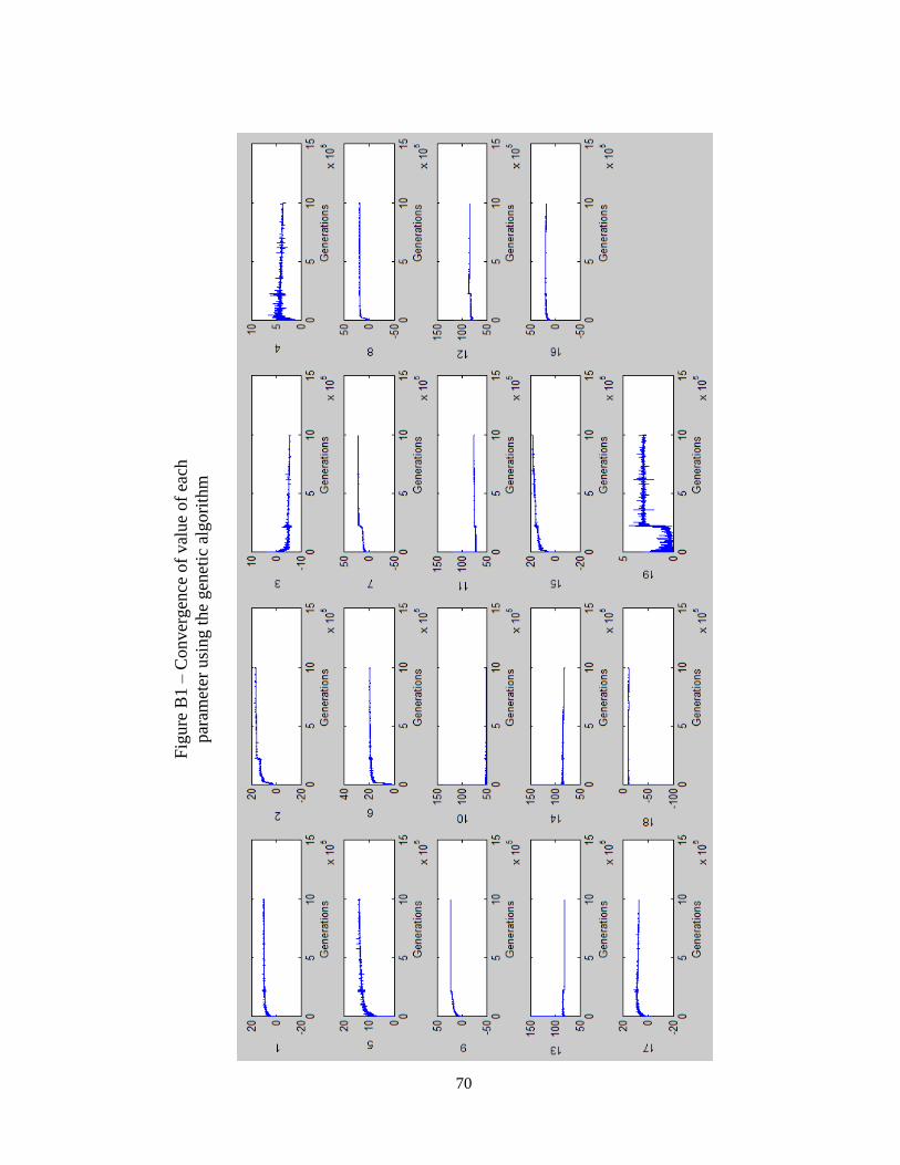
70

Fig

ure

B1 –

Conver

gen

ce o

f val

ue

of

each

par

amet

er u

sing t

he

gen

etic

alg

ori

thm

71

APPENDIX C

DATA ANALYSIS RESULTS FOR ALL RUNS

This section contains the graphs obtained as a result of the data analysis for all the runs.

The following graphs are shown below for each experimental run:

Peak Area for each carbon number obtained from GC

ASF Plot for product distribution

Paraffin, olefin and total Hydrocarbon formation rates for each carbon number

Olefin to paraffin ratio for each carbon number

Run No. 1

Syngas Flow 100 NmL/min, H2/CO ratio 2:1, Bed Temperature 210 °C, CO Conversion 3.07%

0

50000

100000

150000

200000

1 2 3 4 5 6 7 8 9 10 11 12 13 14 15

Pea

k A

rea

Carbon Number

Peak Area v/s Carbon Number

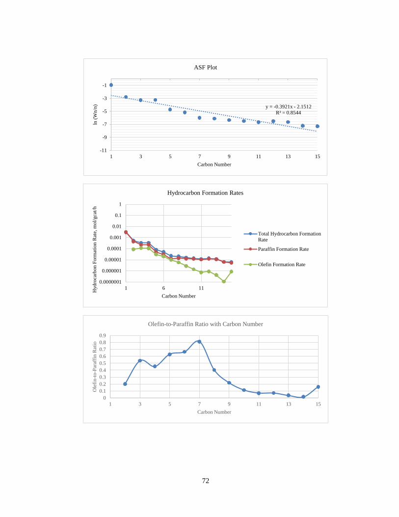
72

y = -0.3921x - 2.1512

R² = 0.8544

-11

-9

-7

-5

-3

-1

1 3 5 7 9 11 13 15

ln (

Wn

/n)

Carbon Number

ASF Plot

0.0000001

0.000001

0.00001

0.0001

0.001

0.01

0.1

1

1 6 11

Hyd

roca

rbon

Form

atio

n R

ate,

mol/

gca

t/h

Carbon Number

Hydrocarbon Formation Rates

Total Hydrocarbon Formation

Rate

Paraffin Formation Rate

Olefin Formation Rate

0

0.1

0.2

0.3

0.4

0.5

0.6

0.7

0.8

0.9

1 3 5 7 9 11 13 15

Ole

fin

-to-P

araf

fin

Rat

io

Carbon Number

Olefin-to-Paraffin Ratio with Carbon Number

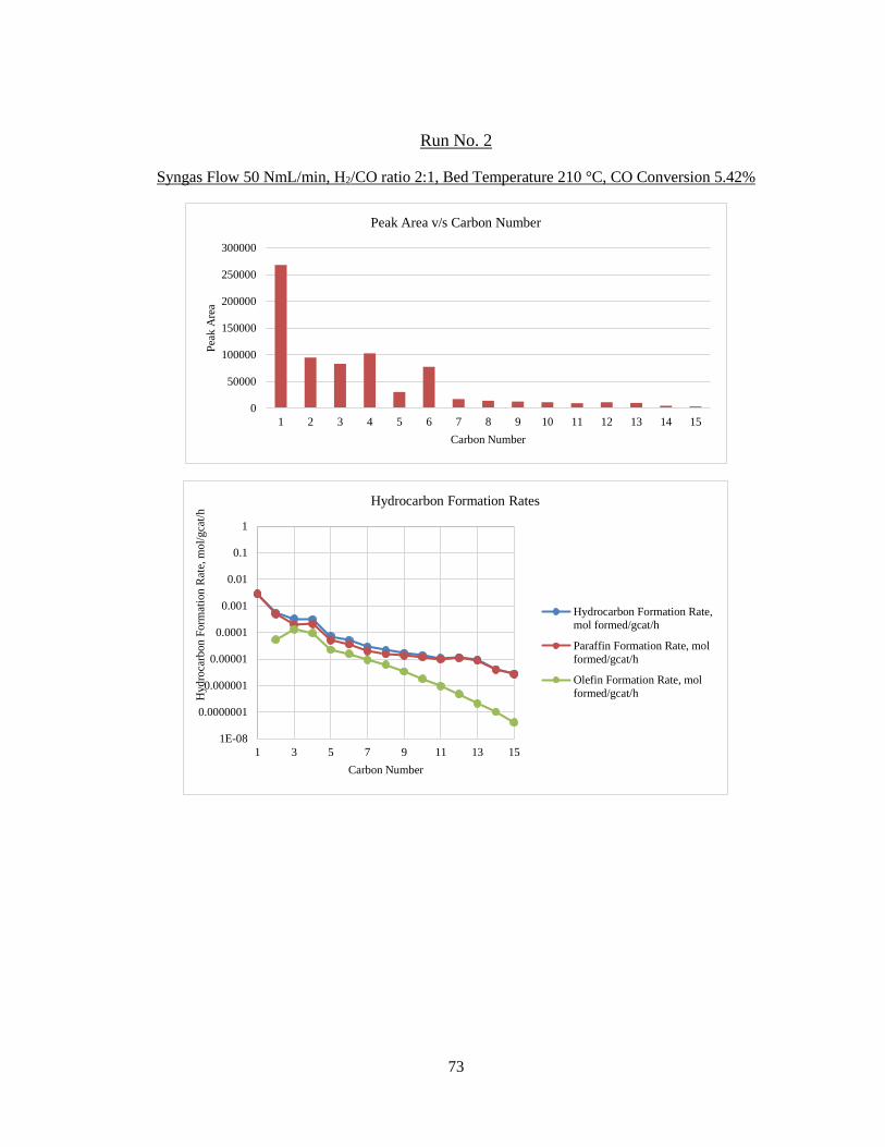
73

Run No. 2

Syngas Flow 50 NmL/min, H2/CO ratio 2:1, Bed Temperature 210 °C, CO Conversion 5.42%

0

50000

100000

150000

200000

250000

300000

1 2 3 4 5 6 7 8 9 10 11 12 13 14 15

Pea

k A

rea

Carbon Number

Peak Area v/s Carbon Number

1E-08

0.0000001

0.000001

0.00001

0.0001

0.001

0.01

0.1

1

1 3 5 7 9 11 13 15

Hyd

roca

rbon

Form

atio

n R

ate,

mol/

gca

t/h

Carbon Number

Hydrocarbon Formation Rates

Hydrocarbon Formation Rate,

mol formed/gcat/h

Paraffin Formation Rate, mol

formed/gcat/h

Olefin Formation Rate, mol

formed/gcat/h

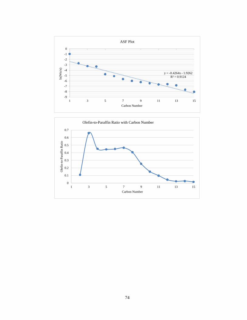
74

y = -0.4264x - 1.9262

R² = 0.9124

-9

-8

-7

-6

-5

-4

-3

-2

-1

0

1 3 5 7 9 11 13 15

ln(W

n/n

)

Carbon Number

ASF Plot

0

0.1

0.2

0.3

0.4

0.5

0.6

0.7

1 3 5 7 9 11 13 15

Ole

fin

-to-P

araf

fin

Rat

io

Carbon Number

Olefin-to-Paraffin Ratio with Carbon Number

75

Run No. 3

Syngas Flow 50 NmL/min, H2/CO ratio 2:1, Bed Temperature 220 °C, CO Conversion 7.97%

0

100000

200000

300000

400000

500000

600000

1 2 3 4 5 6 7 8 9 10 11 12 13 14 15

Pea

k A

rea

Carbon Number

Peak Area v/s Carbon Number

1E-09

1E-08

0.0000001

0.000001

0.00001

0.0001

0.001

0.01

0.1

1

1 3 5 7 9 11 13 15

Hyd

roca

rbon

Form

atio

n R

ate,

mol

form

ed/g

cat/

h

Carbon Number

Hydrocarbon Formation Rates

Hydrocarbon Formation Rate,

mol formed/gcat/h

Paraffin Formation Rate, mol

formed/gcat/h

Olefin Formation Rate, mol

formed/gcat/h

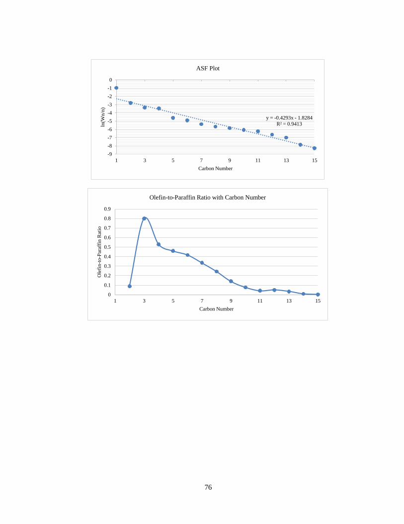
76

y = -0.4293x - 1.8284

R² = 0.9413

-9

-8

-7

-6

-5

-4

-3

-2

-1

0

1 3 5 7 9 11 13 15

ln(W

n/n

)

Carbon Number

ASF Plot

0

0.1

0.2

0.3

0.4

0.5

0.6

0.7

0.8

0.9

1 3 5 7 9 11 13 15

Ole

fin

-to-P

araf

fin

Rat

io

Carbon Number

Olefin-to-Paraffin Ratio with Carbon Number

77

Run No. 4

Syngas Flow 56.85 NmL/min, H2/CO ratio 1.28:1, Bed Temperature 220 °C, CO Conversion

2.76%

0

50000

100000

150000

200000

250000

300000

1 2 3 4 5 6 7 8 9 10 11 12 13 14 15

Pea

k A

rea

Carbon Number

Peak Area v/s Carbon Number

1E-09

1E-08

0.0000001

0.000001

0.00001

0.0001

0.001

0.01

0.1

1

1 3 5 7 9 11 13 15

Hyd

roca

rbon

Form

atio

n R

ate,

mol/

gca

t/h

Carbon Number

Hydrocarbon Formation Rate

Hydrocarbon Formation

Rate, mol formed/gcat/h

Paraffin Formation Rate,

mol formed/gcat/h

Olefin Formation Rate, mol

formed/gcat/h

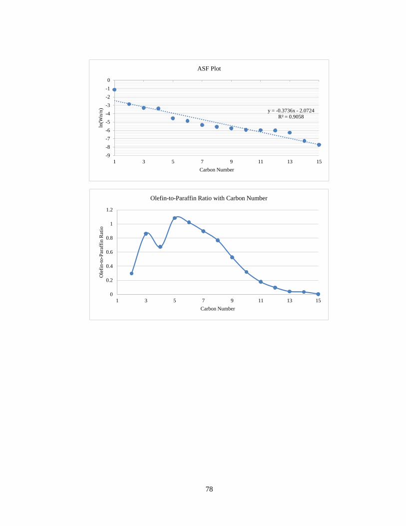
78

y = -0.3736x - 2.0724

R² = 0.9058

-9

-8

-7

-6

-5

-4

-3

-2

-1

0

1 3 5 7 9 11 13 15

ln(W

n/n

)

Carbon Number

ASF Plot

0

0.2

0.4

0.6

0.8

1

1.2

1 3 5 7 9 11 13 15

Ole

fin

-to-P

araf

fin

Rat

io

Carbon Number

Olefin-to-Paraffin Ratio with Carbon Number

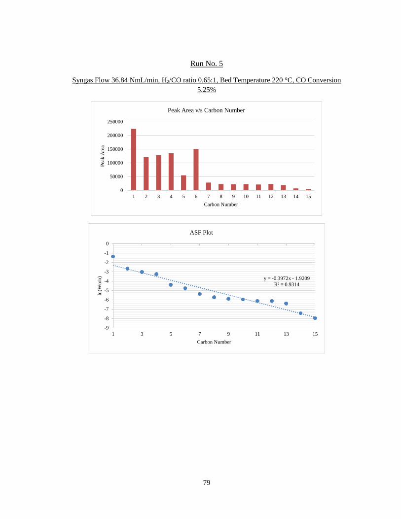
79

Run No. 5

Syngas Flow 36.84 NmL/min, H2/CO ratio 0.65:1, Bed Temperature 220 °C, CO Conversion

5.25%

0

50000

100000

150000

200000

250000

1 2 3 4 5 6 7 8 9 10 11 12 13 14 15

Pea

k A

rea

Carbon Number

Peak Area v/s Carbon Number

y = -0.3972x - 1.9209

R² = 0.9314

-9

-8

-7

-6

-5

-4

-3

-2

-1

0

1 3 5 7 9 11 13 15

ln(W

n/n

)

Carbon Number

ASF Plot

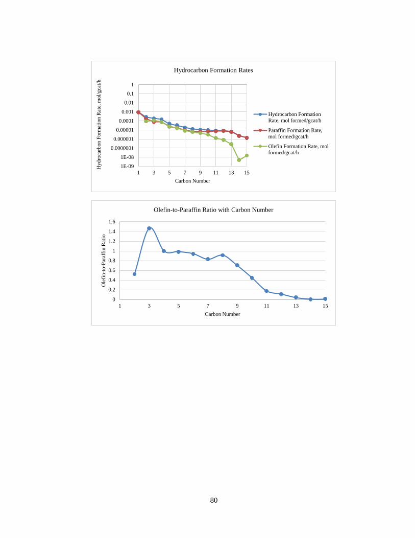
80

1E-09

1E-08

0.0000001

0.000001

0.00001

0.0001

0.001

0.01

0.1

1

1 3 5 7 9 11 13 15

Hyd

roca

rbon

Form

atio

n R

ate,

mol/

gca

t/h

Carbon Number

Hydrocarbon Formation Rates

Hydrocarbon Formation

Rate, mol formed/gcat/h

Paraffin Formation Rate,

mol formed/gcat/h

Olefin Formation Rate, mol

formed/gcat/h

0

0.2

0.4

0.6

0.8

1

1.2

1.4

1.6

1 3 5 7 9 11 13 15

Ole

fin

-to-P

araf

fin

Rat

io

Carbon Number

Olefin-to-Paraffin Ratio with Carbon Number

81

Run No. 6

Syngas Flow 54.43 NmL/min, H2/CO ratio 0.63:1, Bed Temperature 220 °C, CO Conversion

2.57%

0

50000

100000

150000

200000

1 2 3 4 5 6 7 8 9 10 11 12 13 14 15

Pea

k A

rea

Carbon Number

Peak Area v/s Carbon Number

1E-08

0.0000001

0.000001

0.00001

0.0001

0.001

0.01

0.1

1

1 6 11

Hyd

roca

rbon

Form

atio

n r

ate,

mol/

gca

t/h

Carbon Number

Hydrocarbon Formation Rates

Hydrocarbon Formation

Rate, mol formed/gcat/h

Paraffin Formation Rate, mol

formed/gcat/h

Olefin Formation Rate, mol

formed/gcat/h

82

y = -0.414x - 1.8427

R² = 0.9394

-9

-8

-7

-6

-5

-4

-3

-2

-1

0

1 3 5 7 9 11 13 15

ln(W

n/n

)

Carbon Number

ASF Plot

0

0.5

1

1.5

2

2.5

1 3 5 7 9 11 13 15

Ole

fin

-to-P

araf

fin

Rat

io

Carbon Number

Olefin-to-Paraffin Ratio with Carbon Number

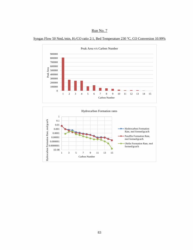
83

Run No. 7

Syngas Flow 50 NmL/min, H2/CO ratio 2:1, Bed Temperature 230 °C, CO Conversion 10.99%

0

100000

200000

300000

400000

500000

600000

700000

800000

900000

1 2 3 4 5 6 7 8 9 10 11 12 13 14 15

Pea

k A

rea

Carbon Number

Peak Area v/s Carbon Number

1E-08

0.0000001

0.000001

0.00001

0.0001

0.001

0.01

0.1

1

1 3 5 7 9 11 13 15

Hyd

roca

rbon

Form

atio

n R

ate,

mol/

gca

t/h

Carbon Number

Hydrocarbon Formation rates

Hydrocarbon Formation

Rate, mol formed/gcat/h

Paraffin Formation Rate,

mol formed/gcat/h

Olefin Formation Rate, mol

formed/gcat/h

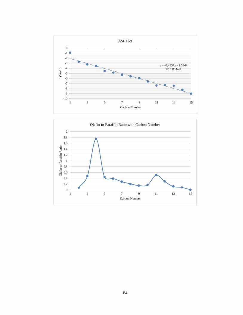
84

y = -0.4957x - 1.5344

R² = 0.9678

-10

-9

-8

-7

-6

-5

-4

-3

-2

-1

0

1 3 5 7 9 11 13 15

ln(W

n/n

)

Carbon Number

ASF Plot

0

0.2

0.4

0.6

0.8

1

1.2

1.4

1.6

1.8

2

1 3 5 7 9 11 13 15

Ole

fin

-to-P

araf

fin

Rat

io

Carbon Number

Olefin-to-Paraffin Ratio with Carbon Number