modeling inﬂuenza viral dynamics in tissue inﬂuenza viral dynamics in tissue ... this paper...

Modeling Influenza Viral Dynamics in Tissue

Catherine Beauchemin1,�, Stephanie Forrest2, and Frederick T. Koster3

1 Adaptive Computation Lab., University of New Mexico, Albuquerque, [email protected]

2 Dept. of Computer Science, University of New Mexico, Albuquerque, NM3 Lovelace Respiratory Research Institute, Albuquerque, NM

Abstract. Predicting the virulence of new Influenza strains is an impor-tant problem. The solution to this problem will likely require a combina-tion of in vitro and in silico tools that are used iteratively. We describethe agent-based modeling component of this program and report prelim-inary results from both the in vitro and in silico experiments.

1 Introduction

Influenza, in humans, is caused by a virus that attacks mainly the upper respi-ratory tract, the nose, throat and bronchi and rarely also the lungs. Accordingto the World Health Organization (WHO), the annual influenza epidemics affectfrom 5% to 15% of the population and are thought to result in 3-5 million casesof severe illness and 250,000 to 500,000 deaths every year around the world [1].The rapid spread of H5N1 avian influenza among wild and domestic fowl andisolated fatal human cases of H5N1 in Eurasia since 1997, has re-awakened inter-est in the pathogenesis and transmission of influenza A infections [2]. The mostfeared strain would mimic the 1918 strain which combined high transmissibil-ity with high mortality [3,4]. Virulence of influenza viruses is highly variable,defined by lethality and person-to-person transmission, but the causes of thisvariability are incompletely understood. The early events of influenza replica-tion in airway tissue, particularly the type and location of early infected cells,likely determine the outcome of the infection. Rate of airway tissue spread iscontrolled by efficiency of viral entry and exit from cells, variable intracellularinterferon activation modulated by the viral NS-1 protein, and by an array of ex-tracellular innate defenses. Although molecular biology has provided a detailedunderstanding of the replication cycle in immortalized cells, influenza replica-tion in intact tissue among phenotypically diverse epithelial cells of the humanrespiratory tract remains poorly understood. We are missing a quantitative ac-counting of kinetics in the human airway and an explanation for how one strain,but not a closely related strain, can initiate person-to-person transmission.

Although the viral structure and composition of influenza are known, and evensome dynamical data regarding the viral and antibody titers over the course ofthe infection [5,6,7], key information such as the shape and magnitude of theviral burst, the length of the viral replication cycle (time between entry of the� Corresponding author.

H. Bersini and J. Carneiro (Eds.): ICARIS 2006, LNCS 4163, pp. 23–36, 2006.c© Springer-Verlag Berlin Heidelberg 2006

24 C. Beauchemin, S. Forrest, and F.T. Koster

first virus and release of the first produced virus), and the proportion of produc-tively infectious virions, is either uncorroborated, unknown, or known with poorprecision. This makes modeling influenza from data available in the literaturea near impossibility, and it points to the need for generating experimental dataaimed directly at the needs of both computational and mathematical models.

This paper describes the computer modeling side of a project that is integrat-ing in vitro experiments with computer modeling to address this problem. We arefocusing on the early dynamics of influenza infection in a human airway epithe-lial cell monolayer using both in vitro and computer models. The in vitro modeluses primary human differentiated lung epithelial cells grown in an air-liquidinterface (ALI) culture to document the kinetics of influenza spread in tissue.The computer model consists of an agent-based model (ABM) implementationof the in vitro system. Its architecture is modular so that more details can beadded whenever data from the in vitro system justifies it. Here, we will describethe implementation of the computer model and report some initial simulationresults.

To our knowledge, only four mathematical models for influenza dynamics haveever been proposed. The first and oldest one is from 1976 and consists of a verybasic compartmental model for influenza in experimentally infected mice [8]. Af-ter a gap of 18 years, Bocharov et al. proposed an exhaustive ordinary differentialequation model based on the basic viral infection model but extended to include12 different cell populations described by 60 parameters [9]. More recently, one ofus co-authored a paper presenting another ordinary differential equation modelwith very slight modifications from the basic viral infection model [10] and asecond paper presenting a simple ABM for influenza [11]. All of these modelseither perform poorly when compared to experimental data or are too simplisticto capture the dynamics of interest in influenza.

2 Agent-Based Modeling

The spatial distribution of agents is an important and often neglected aspect ofinfluenza dynamics. We capture spatial dynamics through the use of an agent-based model (also known as an individual-based) cellular automata style model.Each epithelial cell in the monolayer is represented explicitly, and a computerprogram encodes the cell’s behavior and rules for interacting with other cells andits environment. The cells live on a hexagonal lattice and interact locally withother cells and virions in their neighborhood following a set of predefined rules.Thus, the behavior of the low-level entities is pre-specified, and the simulationis run to observe high-level behaviors (e.g. to determine an epidemic threshold).This style of modeling emphasizes local interactions, and those interactions inturn give rise to the large-scale complex dynamics of interest.

This modeling approach can be more detailed than other approaches. Theprograms can directly incorporate biological knowledge or hypotheses aboutlow-level components. Data from multiple experiments can be combined intoa single simulation, to test for consistency across experiments or to identify gaps

Modeling Influenza Viral Dynamics in Tissue 25

in our knowledge. Through its functional specifications of cell behavior, our canpotentially bridge the current gap between intracellular descriptions and infec-tion dynamics models. Similar approaches have been used to model a varietyof host-pathogen systems ranging from general immune system simulation plat-forms [12,13,14,15,16] to models of specific diseases including tuberculosis [17,18],Alzheimer’s disease [19], cancer [20,21,22,23,24,25], and HIV [26,27].

The spatially explicit agent-based approach is an appropriate method for thisproject. The ALI is a complex biological system in which many different defenses(e.g. mucus, cytokines) interact and biologically relevant values cannot alwaysbe measured directly. In addition, recent high-profile publications have demon-strated that entry of avian and human-adapted influenza viruses into differentairway epithelial cells depends on the cell receptor which in turn is dependent oncell type and location in the airway [28,29]. Our modeling approach will facilitatethe exploration of spatially heterogeneous populations of cells.

3 Influenza Model

Our current model is extremely simple. We plan to gradually add more detail,ensuring at each step that the additions are justified by our experimental data.Here, we describe the model as it is currently implemented.

We are modeling influenza dynamics on an epithelial cell monolayer in vitro.The monolayer is represented as a two-dimensional hexagonal lattice where eachsite represents one epithelial cell. The spread of the infection is modeled byincluding virions. Rather than treat each virion explicitly, the model insteadconsiders the concentration of virions by associating a continuous real-valuedvariable with each lattice site, which stores the local concentration of virionsat that site. These local concentrations are then allowed to change, following adiscretized version of the diffusion equation with a production term. The rulesgoverning epithelial cell and virion concentration dynamics are described below.

3.1 Epithelial Cell Dynamics

The epithelial cells can be found in any of the four states shown in Fig. 1, namelyhealthy, containing, secreting, and dead. For simplicity, we assume that there isno cell division or differentiation over the course of the infection. The parametersresponsible for the transition between these states are as follows.

Infection of Epithelial Cells by Virions (k): Each site keeps track of thenumber of virions local to the site, Vm,n. But while there are Vm,n virions at site(m, n) at a given time step, depending on the length of a time step, not all of thesevirions necessarily come in contact with the cell, and some may contact it morethan once. Alternatively, a particular strain of virions may not be as successfulat binding the cell’s receptors and being absorbed by the cell. To reflect this real-ity, we introduce the parameter k which gives the probability per hour per virion


Infected

DeadHealthy

Containing

τr

τd ± σdSecreting

k, Vm,n

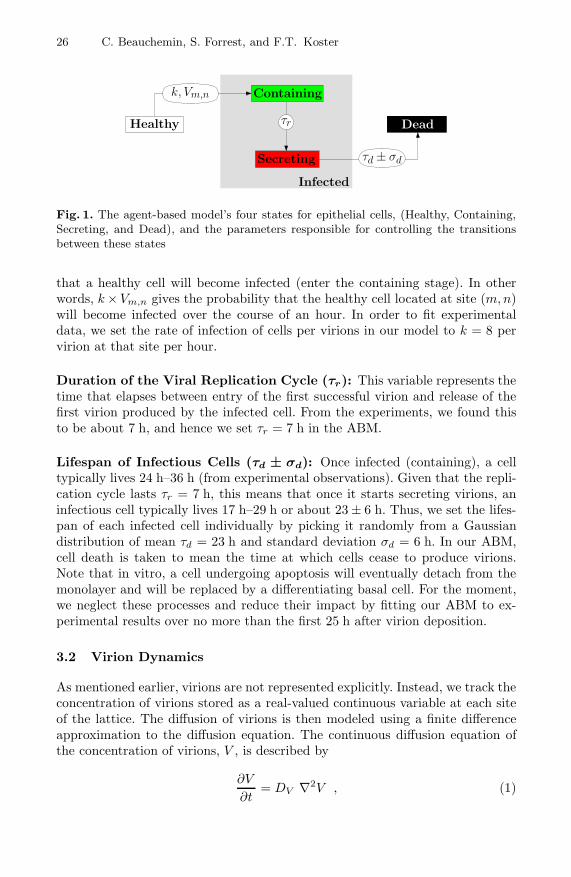
Fig. 1. The agent-based model’s four states for epithelial cells, (Healthy, Containing,Secreting, and Dead), and the parameters responsible for controlling the transitionsbetween these states

that a healthy cell will become infected (enter the containing stage). In otherwords, k ×Vm,n gives the probability that the healthy cell located at site (m, n)will become infected over the course of an hour. In order to fit experimentaldata, we set the rate of infection of cells per virions in our model to k = 8 pervirion at that site per hour.

Duration of the Viral Replication Cycle (τr): This variable represents thetime that elapses between entry of the first successful virion and release of thefirst virion produced by the infected cell. From the experiments, we found thisto be about 7 h, and hence we set τr = 7 h in the ABM.

Lifespan of Infectious Cells (τd ± σd): Once infected (containing), a celltypically lives 24 h–36 h (from experimental observations). Given that the repli-cation cycle lasts τr = 7 h, this means that once it starts secreting virions, aninfectious cell typically lives 17 h–29 h or about 23 ± 6 h. Thus, we set the lifes-pan of each infected cell individually by picking it randomly from a Gaussiandistribution of mean τd = 23 h and standard deviation σd = 6 h. In our ABM,cell death is taken to mean the time at which cells cease to produce virions.Note that in vitro, a cell undergoing apoptosis will eventually detach from themonolayer and will be replaced by a differentiating basal cell. For the moment,we neglect these processes and reduce their impact by fitting our ABM to ex-perimental results over no more than the first 25 h after virion deposition.

3.2 Virion Dynamics

As mentioned earlier, virions are not represented explicitly. Instead, we track theconcentration of virions stored as a real-valued continuous variable at each siteof the lattice. The diffusion of virions is then modeled using a finite differenceapproximation to the diffusion equation. The continuous diffusion equation ofthe concentration of virions, V , is described by

∂V

∂t= DV ∇2V , (1)


where V is the concentration of virions, ∇2 is the Laplacian, and DV is thediffusion coefficient. The simulation is run on a hexagonal grid. The geometryof the grid and the base vectors we chose are illustrated in Fig. 2.

(m, n)

(m,n − 1)

(m + 1, n − 1)

(m + 1, n)

(m,n + 1)

(m − 1, n + 1)

(m − 1, n)�n

�m

√34 Δx

12 Δx

Δx

Fig. 2. Geometry of agent-based model’s hexagonal grid. The honeycomb neighborhoodis identified in gray, and the base vectors m and n are shown and expressed as a functionof Δx, the grid spacing which is the mean diameter of an epithelial cell.

We can express (1) as a difference equation in the hexagonal coordinates(m, n) as a function of the 6 honeycomb neighbors as

V t+1m,n − V t

m,n

Δt=

4DV

(Δx)2

[−V t

m,n +16

∑nei

V tnei

], (2)

such that V t+1m,n at time t+1 as a function of V t

m,n and its 6 honeycomb neighborsV t

nei at time t is given by

V t+1m,n =

(1 − 4DV Δt

(Δx)2

)V t

m,n +2DV Δt

3(Δx)2∑nei

V tnei , (3)

where∑

nei Vtnei is the sum of the virion concentration at all 6 honeycomb neigh-

bors at time t.Because we want to simulate the infection dynamics in an experimental well,

we want the diffusion to obey reflective boundary conditions along the edgeof the well. Namely, we want ∂V

∂j = 0 at a boundary where j is the directionperpendicular to the boundary. It can be shown that for such a case, (3) becomes

V t+1m,n =

(1 − Nnei

2DV Δt

3(Δx)2

)V t

m,n +2DV Δt

3(Δx)2∑Nnei

V tNnei

, (4)


where Nnei is the number of neighbors a cell really has. Note that for Nnei = 6,(4) reduces to (3).

The virion-related parameters DV , Δx, Δt in (4), and the release rate ofvirions, gV , have been set as follows.

Diffusion Rate of Virions (DV ): The diffusion rate or diffusion coefficient forvirions, DV , measures how fast virions spread: the larger DV , the faster virionswill spread to neighboring sites and then to the entire grid. One way to deter-mine DV from experimental results is to take a measure of the “patchiness” ofthe infection, i.e. the tendency of infected cells to be found in batches. The au-tocorrelation function offers a good measure of patchiness. Hence, we calibratedDV by visually matching our simulation to the experimental autocorrelation.We started with DV = 3.18 × 10−12 m2/s which is the diffusion rate predictedby the Stokes-Einstein relation for influenza virions diffusing in plasma at bodytemperature. Ultimately, we found that DV = 3.18 × 10−15 m2/s, a value 1,000-fold greater than the Stokes-Einstein diffusion, yielded the best agreement to theexperimental autocorrelation. This is illustrated in Fig. 3 where the experimentalautocorrelation is plotted against simulation results for different values of DV .

xxxx

xx

xxxx

xx x xx x xx

xx

xx

xxxx

xx xx

xx

x xxxx

0 1 2 3 4 5 6 7 8 9 10 11 12 13 14 15lag (number of sites away)

0.2

0.3

0.4

0.5

0.6

0.7

0.8

0.9

1.0

norm

aliz

ed a

utoc

orre

latio

n

Fig. 3. Autocorrelation at 24 h post-harvest for the experiments (full line, full cir-cles) compared against the autocorrelation produced by the simulation when usinga diffusion coefficient of DV = 3.18 × 10−12 m2/s (dotted line, empty squares), andDV = 3.18 × 10−15 m2/s (dashed line, empty triangles). All parameters are as in Ta-ble 1 except for the DV = 3.18 × 10−12 m2/s simulation where k was set to 4 pervirions per hour to preserve the same fraction of cells infected at 24 h post-harvest.The autocorrelation have been “normalized” to be one for a lag of zero.

Grid Spacing or Diameter of Epithelial Cells (Δx): The diameter ofepithelial cells was estimated from “en face” and cross-section pictures of theexperimental monolayer. The average epithelial cell diameter was found to beabout 11 ± 1 µm. We use Δx = 11 µm.


Duration of a Time Step (Δt): The stability criterion for the finite differenceapproximation to the diffusion equation presented in (4) requires that

Δt ≤ (Δx)2

4DV, (5)

which is a more stringent requirement for larger values of DV or smaller valuesof Δx. We use Δx = 11 µm which is the diameter of lung epithelial cells, andDV = 3.18 × 10−15 m2 · s−1 such that in order to satisfy the stability criterion,we need Δt ≤ 2.6 h. We found that setting Δt = 2 min satisfies the stabilitycriterion of the diffusion equation and accurately captures the behaviour of thesystem.

Virion Release Rate (gV ): As seen above, τr = 7 h after becoming infected,an epithelial cell will start secreting virions. In the model, secreting cells releasevirions at a constant rate until the cell is considered “dead”, at which timesecretion is instantaneously stopped. This “shape” for the viral burst was chosenarbitrarily as very little is known about the shape, duration, and magnitude ofthe viral burst. We found that setting the release rate of virions by secretingcells to gV = 0.05 virions per hour per secreting cell in our ABM yields a goodfit of the simulation to the experimental data.

3.3 Setting Up the Model

The infection of the epithelial cell monolayer with influenza virions in our invitro experiments proceeds as follows. An inoculum containing 50, 000 competentvirions (or 50, 000 plaque forming unit or pfu) is deposited evenly on the cellmonolayer. The solution is left there for one hour to permit the infection of thecells and at time t = 0 h, the inoculum is harvested with a pipette. At thattime, not all the virions are removed: some are trapped in the mucus and getleft behind.

To avoid having to model the initial experimental manipulations and theuncertainty in the viral removal, we start the ABM simulations at time t = 2 hpost-harvest. At that time, a fraction of cells have been infected by the inoculumand a few virions have been left behind at harvest-time. To account for this fact,we define two more parameters, V0 and C0, which give the number of virionsper cell and the fraction of cells in the containing stage at time t = 2 h post-harvest, the initialization time of our simulations. In order to determine thenumber of virions per cell, we also defined Ncells, the number of epithelial cellsin the experimental well. Parameters Ncells, V0 and C0 were set as follows.

Number of Epithelial Cells in the Experimental Well. (Ncells): Wecomputed Ncells, the number of epithelial cells in the experimental well using themeasured diameter of the epithelial cells, Δx = 11 µm, and the known area of theexperimental well, Awell = 113 mm2. Assuming that the sum of the surface area


of all the epithelial cells fully fills the well’s area and that the surface area ofeach cell is roughly circular, such that Acell = π(Δx/2)2, we can compute thenumber of epithelial cells in the experimental well

Ncells =Awell

π (Δx/2)2(6)

=113 mm2

π (11 µm/2)2(7)

∼ 1, 200, 000 cells . (8)

For our ABM, we found that setting the well radius of Rwell = 160 cells, whichcorresponds to about 93,000 simulated cells, is sufficient to accurately capturethe behaviour of a full scale simulation.

Initial Number of Virions per Epithelial Cell (V0): At time t = 2 h post-harvest, the time at which we begin the simulation, 635±273 virions were foundon the monolayer. Hence, we can compute the number of virions per epithelialcell present on the monolayer at time t = 2 h post-harvest,

V0 =635 virions

Ncells(9)

∼ 5.3 × 10−4 virions/cell , (10)

which corresponds to the number of virions per cell at initialization time.

Fraction of Cells Initially Infected (C0): The parameter C0 gives the frac-tion of cells which are initially set to the containing state. Those are the cells thatwere infected during incubation with the inoculum. Staining the ALI monolayerwith viral antigen at t = 8 h post-harvest revealed that approximately 1.8% ofthe cells contained influenza protein, i.e. were producing virions. Hence, we setC0 = 0.018 in the ABM such that 1.8% of cells are set to the containing stageat initialization time.

4 Preliminary Results

In its current implementation, the ABM has 11 parameters shown in Table 1. Ascreenshot of the simulation grid is presented in Fig. 4, and Fig. 5 presents thedynamics of the various cell states and viral titer as a function of time againstpreliminary experimental data. We can see that the ABM provides a reasonablefit to the experimental data.


Table 1. The 11 parameters used in the computer model, with a short descriptionof their role and their default value. In the Source column, C stands for computed,M for measured experimentally, L for taken from the literature, and F for parametersadjusted in order to fit the model to the experiments.

Symbol Description Value SourceFixed Parameters

Rwell radius of simulation well in # cells 160 cells C (Sect. 3.3)Δt duration of a time step 2 min/time step C (Sect. 3.2)Δx grid spacing (diameter of epithelial cells) 11 µm M (Sect. 3.2)τr duration of the viral replication cycle 7 h L (Sect. 3.2)

τd ± σd infectious cell lifespan (mean ± SD) 23 ± 6 h C (Sect. 3.1)Adjusted Parameters

C0 fraction of cells initially infected 0.018 F (Sect. 3.3)V0 initial dose of virions per cell 5.3 × 10−4 virions F (Sect. 3.3)k infection rate of cells by virions 8 /h F (Sect. 3.1)gV rate of viral production per cell 0.05 /h F (Sect. 3.2)DV diffusion rate of virions 3.18 × 10−15 m2/s F (Sect. 3.2)

Fig. 4. Screenshot of the simulation taken at 18 h post-harvest for a simulated grid(well) containing 5, 815 cells using the parameter values presented in Table 1. Thecells are color-coded according to their states as in Fig. 1 with healthy cells in white,containing cells in green, secreting cells in red, and dead cells in black. The magentaoverlay represents the concentration of virions at each site with more opaque magentarepresenting higher concentration of virions.


0 6 12 18 24 30 36 42 48 54 60 66 72time post-harvest (hour)

0.0

0.1

0.2

0.3

0.4

0.5

0.6

0.7

0.8

0.9

1.0

frac

tion

of to

tal c

ells

0 6 12 18 24 30 36 42 48 54 60 66 72

103

104

105

106

vira

l tite

r (p

fu)

Fig. 5. Simulation results using the parameter set presented in Table 1. The linesrepresent the fraction of epithelial cells that are healthy (solid black), containing thevirus (dashed grey), secreting the virus (dashed black), or dead (dotted black), as wellas the number of competent virions (or pfu) on the right y-axis (dash-dot-dot black).The diamonds and the circles represent experimental data for the viral titer and thefraction of cells infected, respectively.Note added in press: Recent experiments have revealed a highly variable dynamic rangeof the replication rate, but the basic structure of the model remains intact.

5 Proposed Extensions

As mentioned earlier, the current model is extremely simple, and we plan togradually increase the level of detail.

One of the first improvements would be the inclusion of different cell types.The epithelial cells that make up the simulation grid are assumed to be a homo-geneous population of cells, with no distinction, for example, between ciliatedand Clara cells. We plan to add more cell types; each cell type would have thesame four states illustrated in Fig. 1, and the transitions between those stateswould still be dictated by the same processes, but the value of the parameterscontrolling these processes would differ from one cell type to another and fromone virus strain to another. With such a model, we could, for example, exploredifferences in the spread of the infection on a sample constituted of 90% cilliatedcells and 10% Clara cells against the spread on a sample constituted of 50%ciliated cells and 50% Clara cells.

We also plan to break existing parameters into sub-models. Let us illustratethis process with an example. At the moment, we describe viral release using theparameter gV which describes the constant rate at which virions are released bysecreting cells. In the future, this simple model of viral release could be replacedby a much more elaborate intracellular sub-model of viral assembly and releasethat takes account of factors such as viral strain and cell type to more accurately


depict the dynamics. These sub-models could either be agent-based simulationsor ordinary differential equations when the spatial distribution of the agentsinvolved is not critical.

We also would like to refine the process of viral absorption, which is currentlydescribed by the parameter k. It has recently been shown [28,29] that suscep-tibility to a particular influenza strain is different depending on the cell type.For example, human influenza virions preferentially bind to sialic acid (SA)-α-2,6-Gal terminated saccharides found on the surface of ciliated epithelial cells ofthe upper respiratory tract while avian influenza H5N1 prefers (SA)-α-2,3-Galfound on goblet cells in and around the alveoli [28,29]. One easy way to take thistype of heterogeneity into consideration would be to define a virion absorptionrate rather than an infection rate, and consider different production rates, gV ,for each strain of virus and for each cell type. Eventually, the parameter forthe absorption rate of virions, for example, could be broken into a sub-modeldescribing the molecular processes involved in virion absorption which wouldexplain in which way virus strains and cell receptors affect its value.

Eventually, when mechanisms such as viral absorption and release have beenmodified to take on the form of molecular sub-models, the ABM will be calibratedagainst a few different known influenza strains. This will provide pointers asto which characteristics of an influenza viral strain drive these mechanisms.Ultimately, we hope to be able to take a newly isolated influenza strain, infectour in vitro system, and then fit our ABM to the experimental results. Doingso would reveal the value of the parameters characterizing this particular strainand hence reveal the lethality and infectivity of that strain.

6 Simulation Platform

The model is implemented on the MASyV (for Multi-Agent System Visualiza-tion) simulation platform. MASyV facilitates the visualization of simulationswithout the user being required to implement a graphical user interface (GUI).The software uses a client-server architecture with the server providing I/O andsupervisory services to the client ABM simulation. The MASyV package con-sists of a GUI server, masyv, a non-graphical command-line server for batch runs,logmasyv, and a message passing library, ma message, containing functions tobe used by the client to communicate with the server. The simulation frameworkis written in C and was developed on a Linux (Debian) system.

With the MASyV framework, a user can write a simple two-dimensional clientprogram in C, create the desired accompanying images for the agents with a paintprogram of her/his choice (e.g. GIMP), and connect the model to the GUI us-ing the functions provided in the message passing library. The flexible GUI ofMASyV, masyv, supports data logging and visualization services, and it supportsthe recording of simulations to a wide range of video formats, maximizing porta-bility and the ability to share simulation results collaborators. The GUI, masyv,is built using GTK+ widgets and functions. For better graphics performance,the display screen widget, which displays the client simulation, uses GtkGLExt’s


OpenGL extension which provides an additional application programming in-terface (API) enabling GTK+ widgets to rapidly render scenes rapidly usingOpenGL’s graphics acceleration capabilities. Capture of the simulation run toa movie file requires the software Transcode [30] and the desired compressioncodecs be installed on the user’s machine.

For non-graphical batch runs, a command-line interface, logmasyv, is alsoimplemented. This option is designed to run multiple simulation runs (e.g. forparameter sweeps on large computer grids). This option requires only that aC compiler be available, and it eliminates the substantial CPU overhead costincurred by the graphical services. Communication between the server program(either masyv or logmasyv) and the client simulation is done through a Unixdomain socket stream.

MASyV is open source software distributed under the GNU General PublicLicense (GNU GPL) and is freely available for download from SourceForge [31].It has a fixed web address, it is well maintained and documented, has an on-line tutorial, and comes with a “Hello World” client simulation demonstratinghow to implement a new client and how to make use of the message passinglibrary. MASyV also comes with a few example pre-programmed clients such asan ant colony laying and following pheromone trails (ma ants) and a localizedviral infection (ma immune) which was used in [11,32]. Our influenza model wasderived from ma immune and is now distributed with MASyV under the namema virions.

7 Conclusion

We have described the implementation of an agent-based simulation built to re-produce the dynamics of the in vitro infection of a lung epithelial cell monolayerwith an influenza A virus. At this time, model development is still in its pre-liminary stage, and many details remain to be elucidated. However, preliminaryruns with biologically realistic parameter values have yielded reasonable resultswhen compared with the currently available experimental data.

Recent results from the in vitro experiments revealed that large numbersof virions were being trapped by the mucus. While at 1 h post-harvest viralassays revealed that the experimental well contained about 4, 701± 180 virions,it contains a mere 635±273 virions only 1 h later at 2 h post-harvest and 720±240virions at 4 h post-harvest. These new results suggest that trapping of the virionsby the mucus and the absorption of virions by the epithelial cells upon infectionplays a crucial role in controlling the rate of spread of the viral infection. Inlight of these new results, we plan to direct our future research towards bettercharacterizing the role of the mucus in viral trapping and its effect on viralinfectivity.

This recent development is an excellent example of just how much we still needto learn about influenza infection. It also shows that our strategy of combiningin vitro and in silico tools will prove a useful tool in this quest.


References

1. World Health Organization: Influenza. Fact Sheet 211, World Health Or-ganization (Revised March 2003) Available online at: http://www.who.int/mediacentre/factsheets/fs211/

2. Webster, R.G., Peiris, M., Chen, H., Guan, Y.: H5N1 outbreaks and enzooticinfluenza. Emerg. Infect. Dis. 12(1) (2006) 3–8

3. Tumpey, T.M., Basler, C.F., Aguilar, P.V., Zeng, H., Solorzano, A., Swayne, D.E.,Cox, N.J., Katz, J.M., Taubenberger, J.K., Palese, P., Garcıa-Sastre, A.: Char-acterization of the reconstructed 1918 Spanish influenza pandemic virus. Science310(5745) (2005) 77–80

4. Tumpey, T.M., Garcıa-Sastre, A., Taubenberger, J.K., Palese, P., Swayne, D.E.,Pantin-Jackwood, M.J., Schultz-Cherry, S., Solorzano, A., Van Rooijen, N., Katz,J.M., Basler, C.F.: Pathogenicity of influenza viruses with genes from the 1918 pan-demic virus: Functional roles of alveolar macrophages and neutrophils in limitingvirus replication and mortality in mice. J Virol 79(23) (2005) 14933–14944

5. Belz, G.T., Wodarz, D., Diaz, G., Nowak, M.A., Doherty, P.C.: Compromizedinfluenza virus-specific CD8+-T-cell memory in CD4+-T-cell-deficient mice. J.Virol. 76(23) (2002) 12388–12393

6. Fritz, R.S., Hayden, F.G., Calfee, D.P., Cass, L.M.R., Peng, A.W., Alvord, W.G.,Strober, W., Straus, S.E.: Nasal cytokine and chemokine response in experimentalinfluenza A virus infection: Results of a placebo-controlled trial of intravenouszanamivir treatment. J. Infect. Dis. 180 (1999) 586–593

7. Kilbourne, E.D.: Influenza. Plenum Medical Book Company, New York (1987)8. Larson, E., Dominik, J., Rowberg, A., Higbee, G.: Influenza virus population

dynamics in the respiratory tract of experimentally infected mice. Infect. Immun.13(2) (1976) 438–447

9. Bocharov, G.A., Romanyukha, A.A.: Mathematical model of antiviral immuneresponse III. Influenza A virus infection. J. Theor. Biol. 167(4) (1994) 323–360

10. Baccam, P., Beauchemin, C., Macken, C.A., Hayden, F.G., Perelson, A.S.: Kineticsof influenza A virus infection in humans. J. Virol. 80(15) (2006)

11. Beauchemin, C., Samuel, J., Tuszynski, J.: A simple cellular automaton model forinfluenza A viral infections. J. Theor. Biol. 232(2) (2005) 223–234 Draft availableon arXiv:q-bio.CB/0402012.

12. Celada, F., Seiden, P.E.: A computer model of cellular interactions in the immunesystem. Immunol. Today 13(2) (February 1992) 56–62

13. Efroni, S., Harel, D., Cohen, I.R.: Toward rigorous comprehension of biologicalcomplexity: Modeling, execution, and visualization of thymic T-cell maturation.Genome Res. 13(11) (2003) 2485–2497

14. Meier-Schellersheim, M., Mack, G.: SIMMUNE, a tool for simulating and analyzingimmune system behavior. arXiv:cs.MA/9903017 (1999)

15. Polys, N.F., Bowman, D.A., North, C., Laubenbacher, R.C., Duca, K.: PathSimvisualizer: An Information-Rich Virtual Environment framework for systems bi-ology. In Brutzman, D.P., Chittaro, L., Puk, R., eds.: Proceeding of the NinthInternational Conference on 3D Web Technology, Web3D 2004, Monterey, Califor-nia, USA, 5–8 April 2004, ACM (2004) 7–14

16. Warrender, C.E.: CyCells. Computer Software distributed on SourceForge underthe GNU GPL at: http://sourceforge.net/projects/cycells. (2005)

17. Segovia-Juarez, J.L., Ganguli, S., Kirschner, D.: Identifying control mechanisms ofgranuloma formation during M. tuberculosis infection using an agent-based model.J. Theor. Biol. 231(3) (2004) 357–376

http://www.who.int/mediacentre/factsheets/fs211/

http://www.who.int/mediacentre/factsheets/fs211/


18. Warrender, C., Forrest, S., Koster, F.: Modeling intercellular interactions in earlyMycobaterium infection. B. Math. Biol. (in press)

19. Edelstein-Keshet, L., Spiros, A.: Exploring the formation of Alzheimer’s diseasesenile plaques in silico. J. Theor. Biol. 216(3) (2002) 301–326

20. Abbott, R.G., Forrest, S., Pienta, K.J.: Simulating the hallmarks of cancer. Artif.Life in press (2006)

21. Gerety, R., Spencer, S.L., Pienta, K.J., Forrest, S.: Modeling somatic evolution intumorigenesis. PLoS Comput. Biol. in review (2006)

22. Gonzalez-Garcıa, I., Sole, R.V., Costa, J.: Metapopulation dynamics and spatialheterogeneity in cancer. PNAS 99(20) (2002) 13085–13089

23. Maley, C.C., Forrest, S.: Exploring the relationship between neutral and selectivemutations in cancer. Artif. Life 6(4) (2000) 325–345

24. Maley, C.C., Forrest, S.: Modeling the role of neutral and selective mutationsin cancer. In Bedau, M.A., McCaskill, J.S., Packard, N.H., Rasmussen, S., eds.:Artificial Life VII: Proceedings of the 7th International Conference on ArtificialLife, Cambridge, MA, MIT Press (2000) 395–404

25. Maley, C.C., Reid, B.J., Forrest, S.: Cancer prevention strategies that addressthe evolutionary dynamics of neoplastic cells: Simulating benign cell boosters andselection for chemosensitivity. Cancer Epidem. Biomar. 13(8) (2004) 1375–1384

26. Strain, M.C., Richman, D.D., Wong, J.K., Levine, H.: Spatiotemporal dynamicsof HIV propagation. J. Theor. Biol. 218(1) (2002) 85–96

27. Zorzenon dos Santos, R.M., Coutinho, S.: Dynamics of HIV infection: A cellularautomata approach. Phys. Rev. Lett. 87(16) (2001)

28. Shinya, K., Ebina, M., Yamada, S., Ono, M., Kasai, N., Kawaoka, Y.: Influenzavirus receptors in the human airway. Nature 440(7083) (2006) 435–436

29. van Riel, D., Munster, V.J., de Wit, E., Rimmelzwaan, G.F., Fouchier, R.A., Oster-haus, A.D., Kuiken, T.: H5N1 virus attachment to lower respiratory tract. Science312(5772) (2006) 399 Originally published in Science Express on 23 March 2006.

30. Ostreich, T., Bitterberg, T., et al.: Transcode. Computer software distributedunder the GNU GPL at: http://www.transcoding.org. (2001)

31. Beauchemin, C.: MASyV: A Multi-Agent System Visualization package.Computer software distributed on SourceForge under the GNU GPL at:http://masyv.sourceforge.net. (2003)

32. Beauchemin, C.: Probing the effects of the well-mixed assumption on viral in-fection dynamics. J. Theor. Biol. in press (2006) Draft available on arXiv:q-bio.CB/0505043.

modeling inﬂuenza viral dynamics in tissue inﬂuenza viral dynamics in tissue ... this paper...

Documents