Sonninal Interest

by Jeffrey C. Fuhrer

No. 95-7 August 1995

Modeling~Lon~-Term

Nominal Interest

by Jeffrey C. Fuhrer

August 1995Working Paper No. 95-7

Federal Reserve Bank of Boston

Modeling Long-Term Nominal InterestRates1

Jeffrey C. FuhrerFederal Reserve Bank of Boston

August 2, 1995

PRELIMINARY DRAFTComments Welcome

Abstract

The Pure Expectations Hypothesis has long served as the pre,eminent bench-mark model of the relationship between the yields on bond~’~i~(of different ma-turities. When coupled with rational expectations, howe~~!;, most empiricalrenderings of the model fail miserably. This paper.explores the possibilitythat failure to account for changes in market participants’ expectations aboutthe monetary policy regime, including changes in the target rate of inflationand the response to inflation and output, may explain much of the failureof the PEH. Estimating explicit expectations fol changing monetary policyregimes in conjunction with the PEH model goes a long way toward rescuingthe PEH model The long rate implied by the PEH for a stationary shortrate process tracks the observed 10ng .rate. The predicted spread betweenthe long and the short rate is highly correlated with the actual spread. Thestandard deviation of the theoretical spread is neatly identical to that ofthe actual spread. Overall, these results cast suspicion on the use of spreadregressions to test the PEH.

1The opinions expressed here are not necessarily shared by the Federal Reserve Bankof Boston or its staff. I thank Alicia Sasser for excellent research assistance.

The most widely-used description of the term structure of interest rates,

the default in both casual and formal conversations among economists, is the

pure expectations hypothesis. The tendency to fall back on this paradigm

is so strong because candidates to replace it are so weak. Relatively minor

differences between observed rates and the predictions of the theory can be

attributed to term or risk premia that vary over time, perhaps in concert with

the state of the business cycle. But the more profound failures of the pure

expectations hypothesis documented by Macaulay (1938), Mankiw (1986),

Mankiw and Miron (1986), Campbell and Shiller (t991), and presented below

are far more dit~icult to explain.

This paper takes a different approach from previous papers to evaluating

the pure expectations hypothesis. Most previous work uses regressions of

the change in a short-term or long-term rate on the spread between the long

and short rates as evidence of the failure of the pure expectations hypothesis.

These regressions tend to demonstrate that, for some maturity combinations,

short rates rise when the long-short spread is high, in conformance with the

pure expectations hypothesis, and long rates tend to fall, in contradiction

to the pure expectations hypothesis (see Campbell and Shiller (1991), Rude-

busch (1995), among others). These papers may be viewed as indirectly

examining the implications of the pure expectations hypothesis.

I more directly explore the implications of the pure expectations hypoth-

esis, by examining the long-term nominal interest rate implied by the pure

expectations hypothesis in conjunction with an explicit description of the

process generating short-term nominal rates. The short rate is determined

by the monetary authority in an attempt to achieve the standard objectives

of monetary policy. In what follows, I will thus summarize Fed behavior as a

"reaction function" in which the federal funds rate responds to deviations of

inflation from a target and to deviations of output around potential, muted

by an interest rate smoothing motive. Market participants will use their esti-

mates of this reaction function, in conjunction with reduced-form equations

for inflation and the output gap, to forecast short-term nominal rates and

thus to determine the appropriate yield on a long-term bond, in conformance

with the pure expectations hypothesis.2

As documented below, if we use the forecasts from a fixed-coefficient

vector autoregression to estimate the long rate implied by the PEH, we obtain

implied iong rates that do not match observed long rates well at all. While

Campbell and Shiller (1991) do not display the long rate implied by the

PEH, their tables of the correlations of the actual and theoretical spreads

and the ratios of their standard deviations tell the same story that I will

tell graphically below. While the correlation between the theoretical and the

actual spread can be fairly high, depending on the maturities involved, the

theoretical spread is generally much less volatile than the actual spread.

The long rates implied by the PEH using forecasts from a fixed-coefficient

VAt~ exhibit the following properties:

1. If short-term nominal rates are mean-reverting (even if they revert quite

slowly), and participants in long bond markets are forward-looking with

long horizons, the pure expectations hypothesis (PEH) predicts a long-

term nominal rate that varies far too little compared to the actual data.

The reason is that during much of the forecast horizon, the short rate is

forecasted to be at or near its mean. Actual long rates exhibit "excess

volatility" relative to the PEH’s predictions.3

2. If short-term nominal rates contain an "important" unit root-i.e., a

2This approach follows the spirit of Hamilton (1988). Hamilton’s results, which asreported supported the PEH, were overturned by Driffil (1992), and thus cannot be con-sidered a "fix" for the PEH.

3Shiller (1979) also documents the excess volatility of the long rate relative to theprediction of the PEH.

unit root that dominates the variance of the series-then, to a first

approximation, the PEH predicts long rates that look like short rates.

The length of market participants’ horizons is nearly irrelevant. Yet

if the Fed targets the rate of inflation (as it almost surely has, at the

very least since 1980), inflation will be stationary. This leaves the

uncomfortable interpretation that most of the variance in long rates

must be attributed to large and permanent shocks to an underlying

long-term equilibrium real rate of interest.4

While it is possible that a reconciliation of the PEH with the data might be

attained by assuming nonstationarity of the short rate, I explore only the

stationary case in this paper.

Considerable effort has been devoted to augmenting the PEH With term

premia and time-varying risk premia. While risk premia certainly exist and

may well vary over time, they are unlikely so explain all of the difference be-

tween the PEH predictions and observed long-term rates. This will become

evident in the following section. I take the approach of Campbell and Shiller

(1991), attempt~ng to ~thoroughly explore the validity of the simple expecta-

tions theory before undertaking a detailed study of the source of predictable

time yariation in excess returns."

This paper pursues a monetary policy-based reconciliation of the data

and the PEH model, as in Mankiw and Miron (19S6), McCallum (1994),Ootsey and Otrok (Z9~5), and Rudebusch (1995). If one is to take the VE~seriously, Jt is essential to understand the process that generates the short-

term nominal interest rate. Since 1966, understanding the behavior of the

short rate has been equivalent to understanding the behavior of the Fed,

which has since that time essentially set the federal funds rate at a target

~Proponents of real business cycle models migh~ find comfor~ in such a proposition.

leve!, in response tO movements in inflation and real activity.5

Unlike McCAlum and l~.udebusch, I do not focus primarily on the im-

plications of particular fixed monetary policy rules for interest rate/spread

regressions across the span of maturities. Unlike McCaIlum (1994), I do

not consider a monetary policy response to a term structure spread itself to

explain apparent conundrums in the data. l~ather, I assume that the Fed

responds only to the standard target variables of inflation and real activity.

My goal is to see if one can use the PEH ~o derive reasonable predictions of

long rates given a monetary policy-determined process for short rates. The

question that this paper addresses is, how bad an approximation is the PEH

for the determination of long-term rates, and can recognition of changes in

Fed behavior make it a better approximation?

The next section depicts graphically ~he resounding failure of the PEH,

using a methodology that is similar to Campbell and Shiller (1987), bu~

focusing on the match between observed long rates and the long rates implied

by the PEH. The second section motivates a structural interpretation of

the failure of ~he PEH: if market participants’ characterization of monetary

policy changes over time, then the PEH predictions of the long rate may not

be as bad as documented elsewhere. The third section presents estimates of

the market’s assumptions abou~ Fed behavior. The fourth section explores

~he implications of the estimated long-term rates for existing empirical work,

and the final section concludes.

SConsiderable debate-focuses on the role of the federal funds rate in the period betweenOctober 1979 and November 1982; it is not widely agr_eed upon how the Fed used thefederal funds rate during this period. See Goodfriend (1993) for detailed exposition of theissues.

1 Another Way of Looking at

the PEH

the Failure of

A simple version of the pure expectations hypothesis makes the ez ante long-

term nominal rate of interest, /~, equal to a weighted average of expected

future short-term nominal interest rates, re over the life of the long-term

bond. For a bond of maturity m,

where the weights wi sum to unity. If we assume a geometric weighting

pattern as in Shiller et aI (1983), then w~ -- (1 -- fl.)fl’ where 0 < ~ _< 1. We

can approximate any finite-maturity bond by an infinite-maturity (consol)

bond with geometric weights that make the duration of the bond equal to the

duration of the flnite-maturity bond. With a constant duration, the consol{

approximation of the finite-maturity bond with duration D is

R~ 1 + D .= 1 ~- D Etr~+~ (2)

This equation says little about how expectations of future short rates

are formed, other than that they are "rational" and based on information

up to and including period t. For this section, I assume that short-term

nominal rates may be well modeled by a four-variable vector autoregression

including the short rate, inflation, the long rate~ and a measure of the output

gap. Defining the vector of variables just described as x~, the VAR may be

written as

¯ ~ = g(L)z~_+ ÷ ~ (3)

where the variable definitions are provided in Table 1, and lag lengths are

chosen accor~ling to conventional criteria.

Rewriting equation 2 in its first-order form

D 1Rt 1 ± DEtR~+I + 1---~-~rt" (4)

Combining this equation with the VAR of equation 3, we can compute the

long-term nominal rates that are consistent with the PEH and with the

stationary vector autoregression.~ Figure ] displays the ex ante long-term

nominal rate computed in this fashion. As the figure shows, the ex ante rate

exhibits far less volatility than the actual ion-g-term rate. The reason is that

the forecasts of the nominal rate from the stationary VAR decay toward their

mean well within the "forecast horizon" for a bond of 7-year duration, so that

for much of the horizon, the funds rate is forecasted to be at its unconditional

mean.

The correlation between the "theoretical" spread and the actual is .68,

indicating that the movemen;s in the implied long rate are often in the right

direction, although as figure 1 indicates, they are far too small. This obser-

vation is consis~en~ with the results for ez ante long-term real rates presented

in Fuhrer and Moore (1995). Thus under the assumption of stationary short-

term rates, the PEtt applied to these maturities is strongly violated by the

da~a. I~ would be possible, but difficult, to imagine time-varying risk premia

of sut~cient magnitude ~o close the gap between the long rates implied by

the PEH in figure 1 and the observed long rates.

The use of a constant-coe~cient VAR implicitly assumes a fixed-coe~cien~

"reaction function" for Fed policy over the entire sample. The contribution

of this paper will be that it allows for changing Fed reaction function co-

eThe method of computing ez ante rates, which is computationally identical to that ofCampbell and Shiller (1987), is described in detail in Fuhrer and Moore (1995).

6

ei~icients across time, and that these estimated changes will be important

enough to reconcile the PEH with the data on longer-term and shorter-term

bonds.

I.I Making Monetary Policy Explicit in the Deter-

mination of Long Rates

Kozicki (1994) examines the PEH model of the term structure in the context

of re-specifying the MIT-PENN-SSI~C (MPS) quarterly model. She observes

the same mismatch of long rate forecasts implied by the PEH and observed

long rates under the assumption of stationary short rate processes. She

ultimately finds a remedy to the problem by using the long end of the term

structure to pin down the "terminal expectation" of market participants.

The intuition is that we can use the implied forward rates contained in long-

maturity bonds to back out the "settling point" for expected future short

rates. The endpoints implied in the long end of the term structure differ

significantly from the unconditional expectations implied by a stationary

VAP~, and the ez ante rates implied by this procedure appear more closely

linked to observed tong rates.

While this procedure works in a mechanical sense, it begs the question of

where the "terminal expectations"--essentially market participants’ uncon-

ditional expectations for nominal rates come from. One would expect the

Fisher equation to hold in the long run, so that

(5)

where T subscripts denote expectations many years out, for example at the

maturity of the longest-term Treasury bonds, and ~rT and PT denote the cor-

responding long-term expectations for inflation and real rates, respectively.

In many structural models, and in the models that I consider here, the

long-run value for inflation is determined solely by monetary policy. In

expectations-augmented Phillips curve and contracting models of price de-

termination, the price specification does not determine the equilibrium level

of inflation. In the simplest version of the expectations augmented Phillips

curve, for example,

= c + + (6)

the specification determines the "non-accelerating-infiation rate of unemploy-

ment" as c!’y, and constrains inflation to equa! expected inflation in equi-

librium. An auxiliary equation, such as a monetary policy function in which

a monetary instrument is set in response to deviations of inflation from a

target, is required to determine the equilibrium level of inflation.

In conformance with these widely-used descriptions of the inflation pro-

tess, I will assume that monetary policy determines the long-term settling

point for inflation. From the perspective of the PEH and the determination

of long-term nominal rates, changes in market participants’ expectatipns of

the monetary authority’s inflation target will alter the expectations of the

"settling point" for short rates, and thus shift the implied long rate.

As important as the ’%ettling point" in determining expectations of future

short rates are the assumed responses of monetary policy.to deviations of

inflation and output from their desired values. For a .given deviation of

inflation from its target, a larger policy response will imply a larger deviation

of the funds rate from its equilibrium. The corresponding argument holds for

a given deviation of output from its equilibrium vMue.~ Thus the market’s

assumptions about policy responses to inflation and output will alter their

expectations of future short rates.

assume throughout that the Fed cannot influence the equilibrium level of real output.

In the sections that follow, I present a simple model that explicitly in-

cludes the Fed’s target inflation rate and that implies an equilibrium real

interest rate. I allow the target inflation rate, the equilibrium real rate,

and the short-run policy responses to shift over different monetary regimes.

I compute the long-term nominal rates implied by the PEH, under the as-

sumption of stationarity, allowing for shifts in the Fed’s inflation target and in

the equilibrium real rMe. I compare the implied rates with these %ndpoint

expectations" identified from the structural model with the estimates pre-

sented in Figure 1, and determine the extent to which allowing for changing

inflation target~ and equilibrium real rates can ~" the gross misbehavior

of the PEH model.

2 A Model of Monetary

Term Interest Rates

Policy and Long-

2.1 Monetary Policy

Monetary policy is modeled as a federal funds rate reaction function, in the

spirit of Fuhrer and Moore (1995) and Taylor (1993). The federal funds rate

responds to deviations of inflation from its target and to deviations of the

output gap from zero

where ~ and/5 are the target and equilibrium rates of inflation and tea! inter-

est rates, and where all of the coefficients may vary across monetary policy

regimes. The lagged funds rate terms allow for an interest rate smoothing

motive on the part of the monetary authority. The final term determines

the ~teady-state value of the funds rate as t’he sum of the equilibrium real

rate and the target inflation rate. The specification for real activity, detailed

below, identifies the equilibrium real rate.

Monetary policy is assumed to follow an equation like 7 throughout the

sample considered here. Market participants are assumed to know the form

of the Fed reaction function, although their estimates of the parameters of

the function can change over time.

2.2 Long Rates

Long-term nominal interest rates are assumed to be determined by the PEH.

The first-order representation of the PEH with rational expectations, equa-

tion 4, defines the implied long-term rate, R~ as

i----0

where the weights ~i are constrained so that the duration of the implied

long-term rate equals the duration, D, of the rate on the lO-year Treasury

constant maturity bond:

For all of the empirical work that follows, I use a constant-duration approxi-

mation, with duration set equal to the average duration for the yield on the

lO-year government constant maturity bond, which is 7 years in my sampl�.

I0

2.3 Inflation and Real Activity

Inflation is defined as the quarterly log change in the GDP deflator. The

output gap is defined as the deviation of log real per capita GDP from a

segmented linear trend with a single breakpoint in 1973 as in Perron (1989).

Both are determined by simple reduced-form equations from a vector au-

toregression (VA!e) with four lags each of inflation, the federal funds rate,

and the output gap. Lag lengths are determined according to conventional

criteria.

3 Market-Perceived Monetary Regime Shifts

and the PEH

Is it conceivable that shifts in market participants’ expectations about mone-

tary policy behavior the target inflation rate and the response of monetary

policy to inflation and output deviations--could alter the long rate implied

by the PEH sufficiently to qualitatively improve Figure 17 The short answer

is yes, changes in these parameters can substantially eliminate the discrep-

ancy between the long rates implied by the PEH and observations on long

rates. The question is whether relatively smooth and plausible shifts in the

bond market’s expectations of the inflation target, the equilibrium real rate,

the response of the funds rate to inflation and real activity, and the degree

of interest rate smoothing can "resurrect" the PEH to respectability.

To answer this question, I perform two exercises. In the first, I take

the VAR equations, for real activity and inflation, and the PEH arbitrage

equation (equation 4) as given. For each observation, I solve for the monetary

policy parameters that make the implied long-term nominal rate from the

PEH "close" to the observed long-term rate. The definition of "closeness"

11

varies across exercises, and I will define two types of closeness below. In

addition, I impose a "smoothness" constraint on the sequence of parameters

so obtained, under the assumption that actual and expected monetary policy

changes occur somewhat gradually.

Formally, the optimization problem may be stated as

+(1- 2} (9)

where 8t is the vector of monetary policy parameters used in period t to

forecast short rates, %-is the relative weight on the "fit" versus the smoothness

of the parameter changes, and w~ are the weights in the moving average of

realized rates.

For the first set of results presented below, I use the squared difference

between a centered nine-quarter moving average of the actual long rate and

the implied long rate from the PEH as the measure of "fit".8 In preliminary

estimates, the interest rate smoothing parameter nearly always took a value

very near unity. Thus the policy reaction function is simplified to

Note that if we set af,~ to 1, the reaction function determines the change in

the funds rate, and knowledge of the equilibrium level of the funds rate is

not required, so fi need not be estimated. The three parameters [a., aN, i]

are chosen to minimize the quantity in equation 9.9

SUsing a trailing eight-quarter moving average does not qualitatively affect theconclusions.

9Setting al,~ to 1 does no~ imply that ~he funds rate has a unit root. It does, however,imply that ~he funds rate moves ~moogl~ly. With any response to the inflation rate (x ~ 0),and with an equilibrium tea! rate determined elsewhere, the nominal rate will settle to thesum of the real rate and inflation in the long run. See ~he discussion in Fuhrer and Moore

12

A second exercise attempts to reconcile the PEH with the bond data

by allowing for a small number of discrete 0no-time Changes in the policy

coefficients. In this exercise, I estimate the VAR across the discrete regime

breaks, allowing the policy coefficients to change at each break, but holding

the rest of the VAIl coefficients constant at their full-sample estimates. I

then compare the long rate implied by the PEH and this model with the

actual long rate data.

3.1 Results: The Implied Long Rate and Reaction

Function Coefficients

Moving Average of Long Rate For these estimates, the optimization

criterion the measure of "closeness" is the squared difference between the

rate implied by the PEH at some parameter settings, and the centered moving

average of the observed !ong nomina] rate. This criterion captures the idea

that the PEH implied rate should equal the observed rate "on average", or

more simply that it should lie approximately on top of the observed rate, but

with somewhat lower volatility.

The results are presented in Figures 2-6; each figure assumes a different

vMue of A, the smoothing coefficient. As the figures demonstrate, relatively

smooth changes in the emphasis on inflation and output in the reaction func-

tion, coupled with a smoothly declining expected inflation target, yield a

PEH-implied long-term nominal rate that tracks the observed tong-term rate

quite closely.1° The pattern of reaction function coefficients is plausible: For

example, during the great disinflation of the early 1980s, the estimated co-

efficient on inflation rises dramatically. The impIied inflati6n target declines

(1995~), especially pages 226-7: for more on this point.1°Table 3 provides the correlations between the actual and the theoretical spreads.

13

substantially over the sample.

No Average For these estimates, the optimization criterion is the squared

difference between the rate implied by the PEH at some parameter settings,

and the observed long nominal rate, This criterion reflects the notion that

the PEH implied rate should equal the observed rate at every point in time.

This leaves essentially no room for time-varying term premia to explain the

differences between yields along the term structure, and thus is equivalent to

the strictest form of the PEH.

Figures 7-8 display the results for this exercise. As expected, the implied

long rate lies even closer ~o the observed long-term rate. Interestingly, the

reaction function coefficients are not terribly different from those for the

exercise above. The general pattern of increased emphasis on inflation in the

early 1980s and a falling inflation target is upheld in these estimates.

These results can be viewed as a successful implementation of the moti-

vation behind Hamilton (1988), later corrected by Driffil (1992). Hamilton

posited different "regimes" for the univariate short rate process that were

distinguished by different time-series properties of the short rate (its mean

and variance). Drlffil showed that, with the proper dataset, these changes

were not sufficient to resuscitate the PEH. The regime shifts here are more

economically motivated, tied ~o changes in monetary policy behavior, and

apparently are sufficient to reconcile the PEH with the data.

3.1.1 Implications for Shorter-Term Rates

While the results discussed above show that modest and plausible changes in

expectations about monetary policy can reconcile the PEH with the 10-year

nominal bond data, these results would be of less interest if they implied

nonsensical behavior for interest rates of other maturities. To put it some-

14

what differently, if entirely different sets of reaction function coefficients were

required to reconcile the PEH with the I- or 2-year maturity nominal bond

yields, the foregoing results would be of little interest to anyone.

I compute the implied 6-month, 1-year, and 2-year rates using the pol-

icy coefficients estimated for the 10-year bond and compare them with the

realized yields. The rates are defined ~s

(10)

where m is the maturity, expressed in quarters, and rl,, is the Z-period

(quarterly) observation on the federal funds rate.

The results are displayed in Figure 9. As the figure shows, the PEH

coupled with the reaction function estimates implies reasonable short- to

medium-maturity yields. This lends more credibility to the reaction function

coef~cients estimated using only data for the !0-year bond.

3.2 A formal estimation of changing monetary policy

regimes

The procedure described above may be viewed as an informal approach

to estimating a "structural VAR" allowing for shifts in the one structural

equation, the policy reaction function. To examine the importance of small

quarter-to-quarter shifts in policy coei~cients for reconciling the PEH with

the data, as compared to discrete one-time changes in coei~icients, I estimate

the VAt{ across four regime breaks, allowing policy coefiicients to change at

each break, but holding the rest of the VAR coei~cients constant at their

full-sample estimates. I add the equation

(11)

15

in order to include the fit of the implied long rate to the observed long rate

data in the estimation. This seems the proper estimation anMogy to the

procedure followed in the previous section.

I choose the break points based on the estimated coefficient patterns

displayed in figures 2-6, so the estimates must be viewed as conditional

on this assumption~ The estimated parameters are summarized in table 2

below,n

The magnitude of the response parameters ~z~ and aN are about the same

as those estimated in the optimization in section 3, and the estimated infla-

tion targets (~) follow a similar pattern. Note that many of the coefficients in

the middle subsamples are not estimated very precisely, although one could

probably Still reject the hypothesis of a constant inflation target throughout.

As figure 10 indicates~ these discrete breaks in expectations about the

three monetary policy parameters are perhaps better than the continuous

time-varying parameters at reconciling the PEH with the 10ng bond data.

Thus the result that accounting for expectations about monetary policy can

"fix" the PEH does not depend on important period-by-period fluctuations

in the implied reaction function coefficients, but rather on a small number of

significant changes in the Fed’s reaction function.

To test the importance of the breakpoints chosen, I also estimate the

same model, with breakpoints in 1979:III and 1982:IV~ corresponding to the

beginning and end of the nonborrowed reserves operating procedure. The

results from this exercise are qualitatively similar to the preceding estimation.

The long-term rate implied by the PEH lies quite close to the actual rate. The

one significant difference is that the implied long rate from these estimates

11A test based on results not shown here indicates that the estimated inflation andoutput response coefficients in the first two subsamples are ihsignificantly different fromone another.

16

"overpredicts" the actual rate in 1990; it gets back on track by 1992. The

implied long-term rate is shown in figure 11.

4 Implications for Existing Empirical Work

4.1 Spread regressions

Following Campbell and Shiller, I regress the long-run change in the short

rate and the short-run change in the long rate on the actual spread and

the theoretical spread. For the time-averaged fitted data, the PEtt holds on

average over a 9-quarter window. For the non-averaged fitted data, the PEI-I

is very close to holding period-by-period. Table 5 displays the results of these

standard regressions.

The results for the actual data conform reasonably well to the results

presented in Campbell and Shiller and elsewhere. Of most interest are the

regressions on the "theoretical" data, which of course conform to ihe pure

expectations hypothesis. The coefficients in the regressions of the long-run

change in the short rate on the spread are all greater than one, although they

are not generally significantly different from one. The coefficient estimates

for the short-run change in the long rate are all negative, although none are

significantly different from zero. Because the PEH must hold by construction

for the theoretical spreads, this exercise casts some suspicion on the usefulness

of the standard spread regressions.

In one sense, these results confirm those of l~udebusch (1995). Because

the spread may be expressed as the expectation of the weighted sum of the

first-differences of future short rates, the coefficient in the test regression de-

pends critically on the predictability of the change in the short rates, l~ude-

busch finds thai if the Fed behaves in such a way as to make first-differences

17

of the funds rate not very predictable (at least over some horizons), then the

estimated spread coefficient in the test regression will be close to zero. In

a sense, this paper makes the more general point that discrete shifts in Fed

behavior can make mush of the standard test regressions, even though the

PEH holds almost exactly in every period.

4.2 Comparisons of Actual and Theoretical Spreads

The ratios of the standard deviation of the theoretical spread to the actuM

spread are reported in Table 4. In Campbell and Shiller (1991), these ratios

for bonds of 10-year maturity cluster around .5. For the theoretical spreads

computed in this study, the standard deviation ratios are all quite close to

one. Thus the realized spreads do not exhibit excess volatility relative to

the theoretical spreads, once changes in policy are accounted for. This result

overturns the result in Campbell and Shiller (1991).

Finally, the correlations between the actual and the theoretical spreads

are of interest. Recall that in Campbell and Shiller, the correlations for this

maturity spread were quite high. Here, for the variety of PEH-consistent

spreads generated above, the correlation between the actual and the the-

oretical spread ranges from 0.89 to 0.99. By this metric, the PEH with

smoothly-evolving poticy parameters fits the data markedly better than the

fixed-coefficient alternative.

4.3 How wrong could market expectations be?

If market participants had used the smoothly-evolving reaction function pa-

rameters estimated above to predict the funds rate, how far wrong would

they have gone? The structural VAR estimates above suggest that the PEH-

consistent reaction function coefficients could not be too far off, since the

18

structurM VAR estimates fit both" the data on the funds rate and the long

rate, and they appear to be not very different from the PEH-consistent esti-

mates. But could a well-informed research department have shown "market

participants" that their estimates of the policy response were statisticallyuntenable?

I will not attempt a formal statistical test of this hypothesis here, as it

is not obvious what the regression model that nests the fitting exercise of

section 3 looks like. Instead, I will use two heuristic measures to address the

question.

4.3.1 Information in the Funds Rate Prediction Errors

The first heuristic looks at errors made in predicting the funds rate with the

evolving parameter estimates. If the predicted funds rate deviates signifi-

cantly and persistently from the actual funds rate, then market participants

would have been obviously foolish to use these estimates, and could have

adjusted their estimates based on the structure in the prediction errors.

Figure 12 shows the autocorrelation functions for the predicted funds

rates using estimates of the policy parameters for different smoothing pa-

rameters. As the figure shows, there is no strong evidence of structure in

the prediction errors. There are just-significant autocorretations ~at lags two

and seven, both with magnitude of about .2. Thus the impli.ed funds rate

estimates from the time-varying parameters fit the actual funds rate data

reasonably well.

4.3.2 Rolling regression estimates of reaction function

The second heuristic compares the sequence of reaction function parame-

ter estimates obtained in section 3 with rolling regression estimates of the

same parameters. Statistically, these estimates are not perfectly compatible,

19

because the rolling regression estimates assume fixed parameters, while the

PEHt-consistent estimates explicitly assume time-varying parameters. Still,

one can get a sense of what the estimated parameters from a widely-used

technique look like compared to the PEH-consistent parameters, and whether

they point to entirely different reaction function parameter estimates or to

greater parameter stability.

Figure 13 displays the rolling regression parameter estimates for a 10-year

data window for each of the three policy parameters, along with the PEI-I-

consistent estimates for )~ - .2 presented above. As the figure indicates, the

range of estimates that arise from the rolling-regression methodology easily

spans the estimates that arise from the optimization in section 3. Only in the

early 1980s do the response coefficients fall outside ~he 2-standard-error bands

around the rolling-regression estimates. However, the rolling-regression es-

timates themselves are a bit suspect during this period: as they imply that

the Fed responded so as to reinforce rather than to lower inflation during the

time of the great disinflation. By this simple gauge, then, the PEH-consistent

policy parameters cannot be ruled out as statistically untenable.

5 Conclusion

The PEH imposes a very tight linkage between the process-assumed to gener-

ate short-term nominal rates and the realizations of long-term nominal rates.

As a result, a careful examination of the determinants of the short-term nomi-

nal rate is warranted. This paper takes the position that the primary-indeed,

the sole-determinant of short nominal rate behavior is the behavior of the

Federal l~eserve. Thus a careful examination of the Fed’s reaction function,

and how it has changed over time, is required to understand the implications

of the PEH for long rates.

20,

Using a simple framework that uses reduced-form equations for inflation

and output~ combined with a very simple Fed reaction function and the PEH,

I find that changes in the Fed’s behavior over time can reconcile the PEH

with the interest rate data quite nicely. In particular, the interest rates ofvarious maturities that are implied By the PEI-I are highly correlated with

their observed counterparts and exhibit nearly the same volatility. Thus, inCampbell and Shiller~s terms, both the correlation Between the theoretical

and actual spread and the ratio of the standard deviations of the theoretical

and actual spreads are close to one.This paper also demonstrates that simple spread regression tests of the

PEH may be very misleading. When monetary policy alters the process

generating the short-term interest rate, there is little reason to believe thatthe coef~cient in the canonical test regression should be one. In data for

which the PEH is shown to hold nearly exactly, the test regressions yield

coef~cients not significantly different ~rom zero.Thus the Pure Expectations Hypothesis of the term structure may not

be as awful as many empirical investigations have suggested. In fact~ thispaper develops results that suggest that it is a very good approximation of

long-term bond behavior. The key to understanding previous failures of the

PEH is in understanding the process that generates the short-term nominalinterest rate. If allowance is made for shifts in the process used to form

expectations of future short-term rates, then the PEH fares quite well.

21

References

[1] John Y. Campbell. Some Lessons From the Yield Curve. Working PaperSeries 5031, NBER, February 1995.

[2] John Y. Campbell and John Ammer. What Moves the Stock and Bond

Markets? A Variance Decomposition for Long-Term Asset Returns.

Journal of Finance, 48:3-37, 1993.

[3] John Y. Campbe11 and Robert J. Shiller. Cointegration and Tests

Present Value Models. Journal of Political Economy, 95:1062-1088,

1987.

[4] John Y. Campbell and Robert J. Shiller. Yield spreads and interest rate

movements: a bird’s eye view. Review of Economic Studies, 58:495-514,

1991.

[5] Michael Dotsey and Christopher Otrok. The Rational E-xpectations

Hypothesis of the Term Structure, Monetary Policy, and Time-Varying

Term Premia. Federal Reserve Bank of Richmond Economic Quarterly,

81/1, Winter:65-81, 1995.

[6] John Driffil. Changes in Regime and the Term Structure: A Note.

Journal of Economic Dynamics and Control, 16:165-173, 1992.

[7] Kenneth A. Froot. New Hope for the Expectations Hypothesis of the

Term Structure of Interest Rates. Journal of Finance, 44:283-305, 1989.

[8] Jetgrey C. Fuhrer and George 1~. Moore. Monetary Policy Trade-Offs

and the Correlation Between Nominal Interest Rates and Real Output.

American Economic Review, 85:219-239, March !995.

22

[9]

[10]

[11]

[12]

Marvin Goodfriend. Interest rate policy and the inflation scare problem:

1979-1992. Federal Reserve Bank of Richmond Economic Quarterly,

79/1:1-24, 1993.

James Hamilton. Rational Expectations Econometric Analysis of

Changes in Regime: An Investigation of the Term Structure of Interest

Rates. Journal of Economic Dynamics and Control, 12:385-423, 1988.

Sharon Kozicki. Modeling Long-Term Nominal Interest Rates in the

MPS Model. Working Paper, Board of Governors of the Federal Reserve

System, December 1994.

Frederick R. Macaulay. Some Theoretical Problems Suggested by the

Movements of Interest Rates, Bond Yields, and Stock Prices in the

United States Since 1856. NBER Working Paper Series, New York,

1938.

[13]

[14]

[15]

[16]

[17]

N. Gregory Mankiw. The Term Structure of Interest Races Revisited.

Brookings Papers on Economic Activity, 1:61-110, 1986.

N. Gregory Mankiw and Jeffrey A. Miron. The Changing Behavior of

the Term Structure of Interest Rates. Quarterly Journal of Economics,

101(2):211-228, May 1986.

Bennett T. McCallum. Monetary Policy and the Term Structure of

Interest Rates, August 1994. Working Paper.

Frederick S. Mishkin. The Information in the Longer-Maturity Term

Structure About Future Inflation. Quarterly Journal of Economics,

105:815-821, 1990.

Pierre Perron. The Great Crash, the Oil Price Shock and the Unit Root

Hypothesis. Econometrica, 57:1361-1401, 1989.

23

[18]

[19]

[21]

Glenn D. Rudebusch. Federal Reserve Interest Rate Targeting, Ratio-

nal Expectations, and the Term Structure, February 1995. FRB San

Francisco Working paper, forthcoming do~zal of Monet~d Economics.

Robert J. Shiller. The Volatility of Long-Term Interest Rates and Ex-

pectations Models of the Term Structure. Jo~r~gl of Polit~c~l F~conora~,

87/6:1190-1219, 1979.

Robert J. Shiller, John Y. Campbell, and Kermit L. Schoenholtz. For-

ward Rates and Future Policy: Interpreting the Term Structure of In-

terest Rates. Brookinps P~pers on .~con, o~c Ac~ivi~l, 1:173-223, 1983.

John B. Taylor. Discretion Versus Policy Rules in Practice. Ugr~zegie-

!~oclzestev Conference Sev~es or, Public Polic~, 39:195-214, 1993.

24

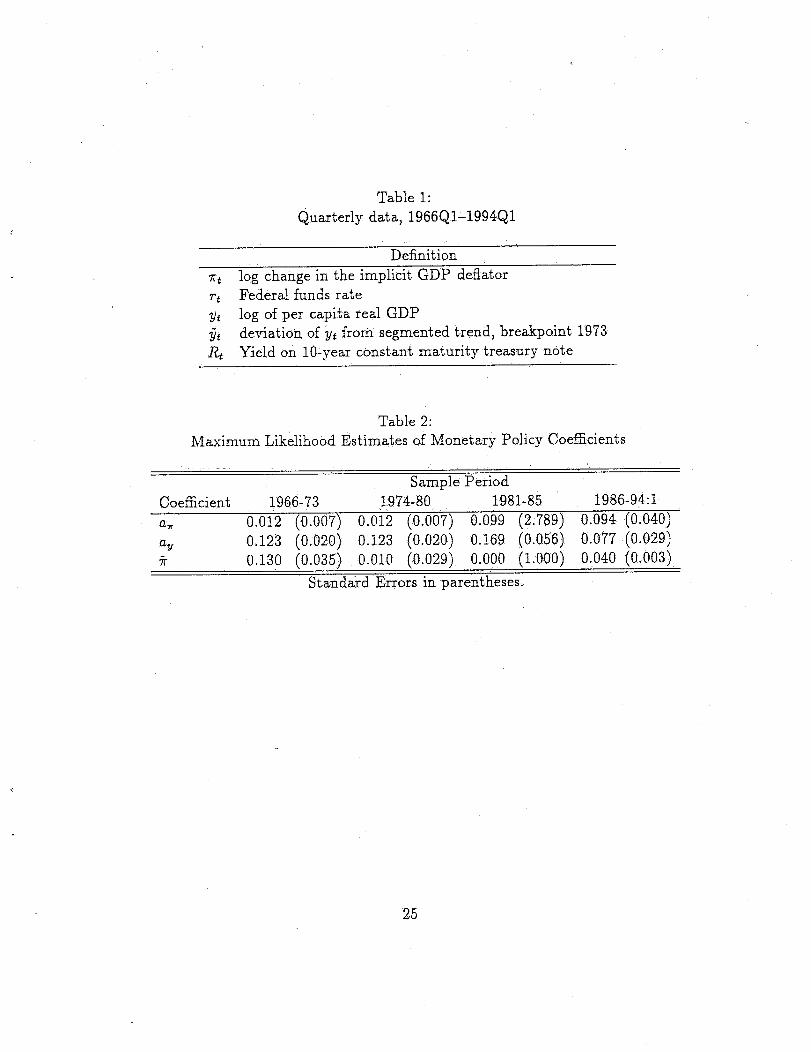
Table 1:Quarterly data, 1966QI-1994Q1

Definition

log change in the implicit GDP deflatorFederal funds ratelog of per capita real CDPdeviation of ~4 from segmented trend, breakpoint 1978Yield on 10-year constant maturity treasury note

Table 2:Maximum LikelihoOd Estimates of Monetary Policy Coefficients

Sample PeriodCoefficient 1966-73 1974-80 1981-85 1986-94:1a. 0.012 (0.007) 0.012 (0.007) 0.099 (2.789) 0.094 (0.040)% 0.123 (0.020) 0.123 (0.020) 0.169 (0.056) 0.077 (0.029)~- 0.130 (0.035) 0.010 (0.029) 0.000 (i.000) 0.040 (0.003)

Standard Errors in parentheses.

Table 3:

Correlation of Theoretical and Actual Spread

Fit ~o Moving AVerage

0.05 0.10 0.20 0.30 0.50.96 .96 .95 .93 .87

Fit to Da~a

0.05 0.10 0.20 0.30 0.50.99 .98 .96 .94 .89

FIML estimates, 4 regimes.93

Table 4:

Ratio of Standard Deviations of Theoretical to Actual Spread

Fit to Moving Average

0.05 0.10 0.20 0.30 0.501.09 1.08 1.09 1.10 1.12

Fit to Data

0.05 0.10 0.20 0.30 0~50.99 1.02 1.06 1.08 1.12

FIML estimates, 4 regimes.91

26

Table 5:Campbelt-Shiller Test Regressions

Dependent variable: 10-year change in short rateActual Spread

Weight on Smoothing (~) Coeff. Stand. Error

0.05 1.08 0.290.i00.200.300.50

FIMLDependent variable: Change in long rate

0.05 -1.76 0.770.100.200.300.50

FIML

The regression for the top panel

Theoretical SpreadCoei~. Stand. Error

1.09 0.241.12 0.251.12 0.261.17 0.261.30 0.23i.I0 0.30

-0.56 0.73-0.47 0.73-0.53 0.73-0.52 0.72-0.29 0.71-1.67 0.78

is:

~] rt+~/(m - 1) - r, -- c + b((rn - 1)/rn)S’t

The regression for the bottom panel is:

where m is the maturity of the long bond in quarters and S~ is the G-periodobservation on the spread between the long yield and the short yield.

27

1.1.1

Figure 2

Long Rates and Reaction Function Coefficients Implied byPEH, Smoothing Coefficient = .05Fit Moving Average of 10-Year Rate

Percent16%

14%

12%

10%

8%

6%

Actual v. PEH Long Rates

Actual

PEH

4%66Q1 68Q1 70Q1 72Q1 74Q1 76Q1 78Q1 80Q1 82Q1 84Q1 86Q1 88Q1 90Q1 92Q1

Percent16%

14%

12%

10%

8%

6%

4%

Reaction Function Coefficients

Inflation Response

Output Response

66Q1 68Q1 70Q1 72Q1 74Q1 76Q1 78Q1 80Q1 82Q1 84Q1 86Q1 88Q1 90Q1 92Q1

Pe~e~10%

8%

4%

2%

Inflation Target

66Q1 68Q1 70Q1 72Q1 74Q1 76Q1 78Q1 80Q1 82Q1 84Q1 86Q1 88Q1 90Q1 92Q1

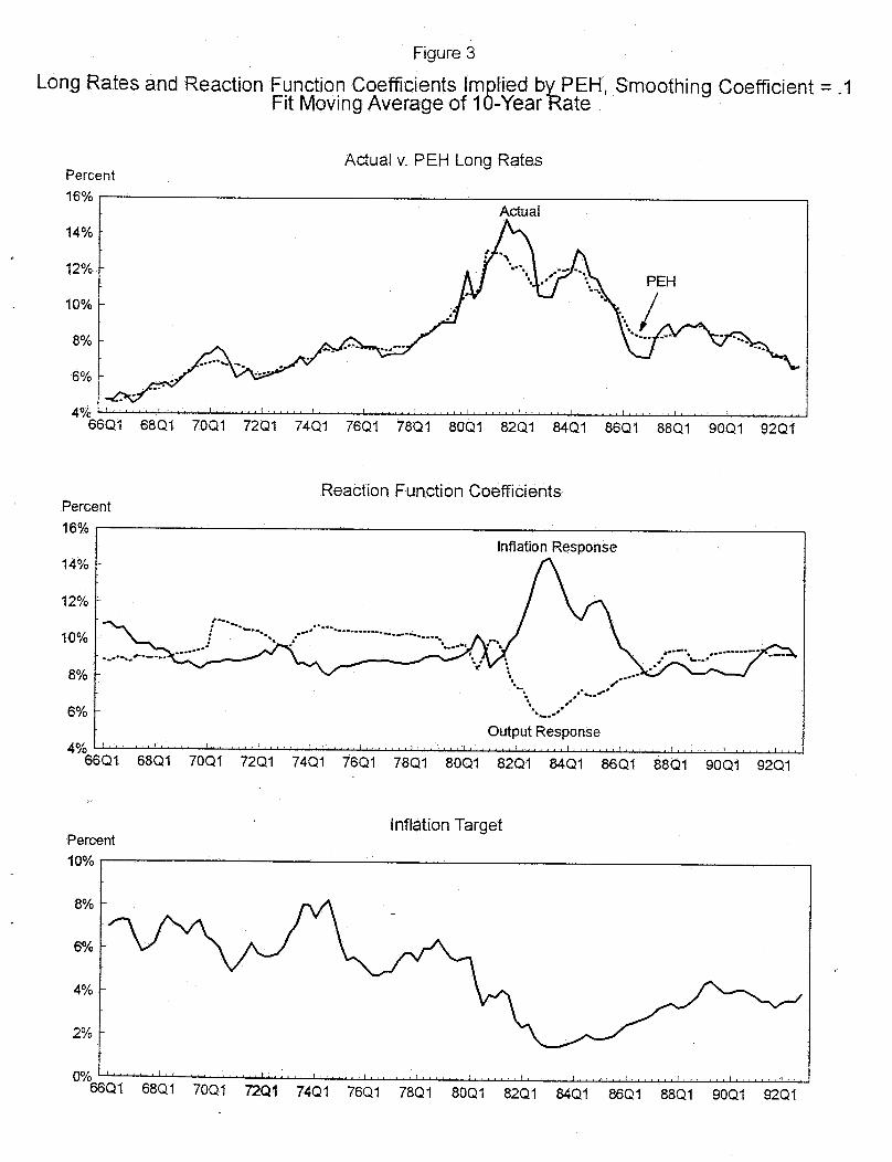
Figure 3

Long Rates and Reaction Function Coefficients Implied byPEH,Fit Moving Average of 10-YearRate

Smoothing Coefficient = .1

PercentActual v. PEH Long Rates

16%

14%

12%

10%

8%

6%

4%66Q1

Actual

68Q1 70Q1 72Q1 74Q1 76Q1 78Q1 80Q1 82Q1 g4Q1 86Q1 88Q1 90Q1 92Q1

Reaction Function CoefficientsPement16%

14%

12%

10%

8%

6%

4%66Q1

Inflation Respon se

Output Response

68Q1 70Q1 72Q1 74Q1 76Q1 78Q1 80Q1 82Q1 84Q1 86Q1 88Q1 90Q1 92Q1

Percent10%

Inflation Target

8%

4%

2%

66Qt 68Q1 70Q1 72Q1 74Q1 76Q1 78Q1 80Q1 82Q1 84Q1 86Q1 88Q1 90Q1 92Q1

Figure 4

Long Rates and Reaction Function Coefficients Implied by PEH, Smoothing CoefficientFit Moving Average of 10-YearRate

= ,2

Actual v. PEH Long RatesPercent

16%

14%

12%

10%

8%

6%

4%66Q1

Actual

~ t~//EH

68Q1 70Q1 72Q1 74Q1 76Q1 78Q1 80Q1 82Q1 84Q1 86Q1 88Q1 90Q1 92Q1

Reaction Function CoefficientsPercent18%

16%

14%

12%

10%

8%

6%66Q1

Inflation Response

Output Response

68Q1 7001 7201 7401 7601 7801 8001 8201 8401 8601 8801 90Q1 9201

Percent8%

7%

6%

5%

4%

3%

2%

1%66Q1

Inflation Target

68Q1 70Q1 72Q1 74Q1 76Q1 78Q1 80Q1 82Q1 84Q1 86Q1 88Q1 90Q1 92Q1

Figure 5

Long Rates and Reaction Function Coefficients Implied byPEH, Smoothing Coefficient = .3Fit Moving Average of 10-Year Rate

Actual v; PEH Long RatesPercent16%

14%

12%

10%

8%

Actual

, i~/tEl’4 "

6%

4 6 1-’°6°’Q" ...........................6801 7001 720174 1 -Q-6-’7 Q1 .............7801 8001’ .......8201’ .......8401’ .......8601’ .......8801’ ...................900i 9201

Percent16% I

14%

Reaction Function Coefficients

Inflation Response

12%

10%

8%Output Response

6%66Q1 68Q1 70Q1 72Q1 74Q1 76Q1 78Q1 80Q1 82Q1 84Q1 86Q1 88Q1 90Q1 92Q1

Percent8%

Inflation Target

7%

5%

4%

3%

2%

1% ,t,, ..... , .......66Q1 68Q1 FOQ1 72Q1 74Q1 76Q1 78Q1 80Q1 82Q1 84Q1 86Q1 88Q1 90Q1 92Q1

Figure 6

Long Rates and Reaction Function Coefficients Implied by PEH, Smoothing Coefficient = .5Fit Moving Average of 10-YearRate ~

Percent16%

14%

12%

10%

8%

6%

Actual v. PEH Long Rates

Actual

PEH

4%66Q1 68Q1 70Q1 72Q1 74Q1 76Q1 78Q1 80Q1 82Q1 84Q1 86Q1 88Q1 90Q1 92Q1

Percent12%

11.5%

11%

10.5%

10%

9.5%

9%

8.5%

8%66Q1

Reaction Function Coefficients

Inflation Response

,O,~l:)ut Res,ponse

68Q1 70Q1 72Q1 74Q1 76Q1 78Q1 80Q1 82Q1 84Q1 86Q1 88Q1 90Q1 92Q1

Percent8%

Inflation Target

7%

6%

5%

4%

3%

66Q1 68Q1 70Q1 72Q1 74Q1 76Q1 78Q1 80Q1 82Q1 84Q1 86Q1 88Q1 90Q1 92Q1

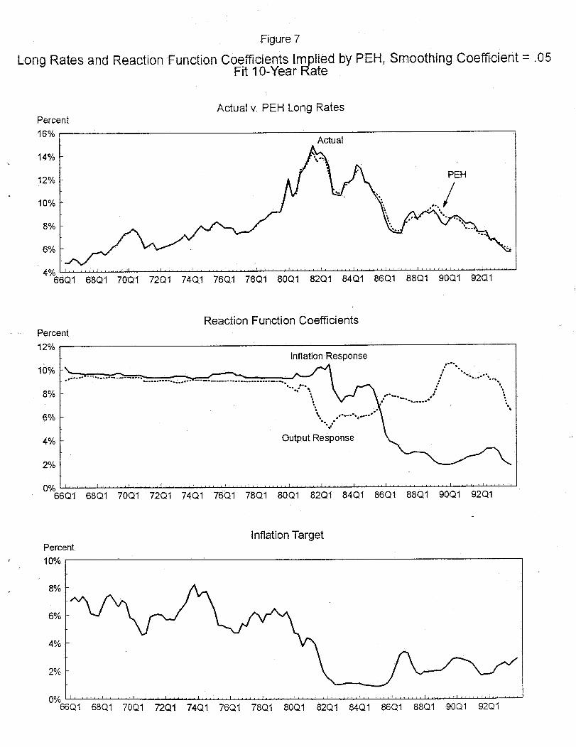
Figure 7

Long Rates and Reaction Function Coefficients Implied by PEH, Smoothing Coefficient = .05Fit 10-Year Rate

Actual v. PEH Long RatesPercent16%

14%

12%

10%

8%

6%

Actual

66Q1 68Q1 70Q1 72Q1 74Q1 76Q1 78Q1 80Q1 82Q1 84Q1 86Q1 88Q1 90Q1 92Q1

Reaction Function CoefficientsPercent12%

10%

8%

6%

4%

2%

Inflation Response

....... ,, ...........~...." ................’....~ .......J*J~.

output-’’/- e

66Q1 68Q1 70Q1 72Q1 74Q1 76Q1 78Q1 80Q1 82Q1 84Q1 86Q1 88Q1 90Q1 92Q1

Percent10%

8%

6%

4%

2%

Inflation Target

66Q1 68Q1 70Q1 72Q1 74Q1 76Q1 78Q1 80Q1 82Q1 84Q1 86Q1 88Q1 90Q1 92Q1

Figure 8

Long Rates and Reaction Function Coefficients Implied by PEH, Smoothing Coefficient = .5Fit I 0-Year Rate

Percent16%

14%

12%

10%

8%

6%

4%

Actual v. PEH Long Rates

Actual

PEH/

/

66Q1 68Q1 70Q1 72Q1 74Q1 76Q1 78Q1 80Q1 82Q1 84Q1 86Q1 88Q1 90Q1 92Q1

Reaction Function CoefficientsPercent12%

11%

10%

Inflation Response

9% Output Response- ~’"’-,,

66Q1 68Q1 70Q1 72Q1 74Q1 76Q1 78Q1 80Q1 82Q1 84Q1 86Q1 88Q1 9001 92Q1

Percent8%

7%

6%

5%

4%

3%

2%

Inflation Target

66Q1 68Q1 70Q1 72Q1 74Q1 76Q1 78Q1 80Q1 82Q;I 84Q1 86Q1 88Q1 90Q1 92Q1

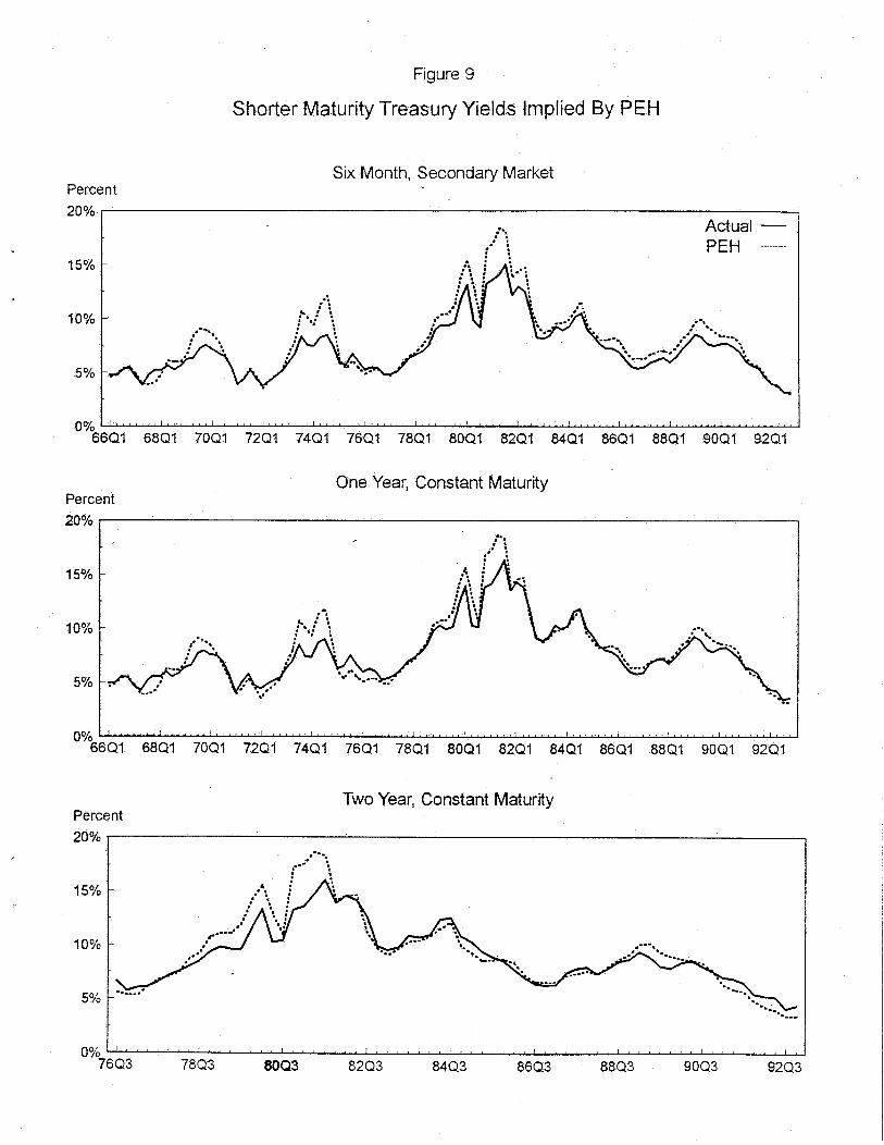
Figure 9

Shorter Maturity Treasury Yields Implied By PEH

Percent20%

15%

10%

5%

Six Month, Secondary Market

;., Actual¯ - PEH .........

66Q1 68Q1 70Q1 72Qt 74Q1 76Q1 78Q1 80Q1 82Q1 84Q1 86Q1 88Q1 90Q1 92Q1

Percent20%

15%

10%

5%

One Year, Constant Maturity

66Q1 68Q1 70Q1 72Q1 74Q1 76Q1 78Q1 80Q1 82Q1 84Q1 86Q1 88Q1 90Q1 92Q1

Two Year, Constant MaturityPercent20%

15%

10%

5%

76Q3 78Q3 80Q3 82Q3 84Q3 86Q3 88Q3 90Q3 92Q3

Percent

16%

Figure 10

Actual and PEH-Implied Long Rates, from FIML Estimates

14%

12%

10%

6%

PEH

;

Actual

66Q1 68Q1 70Q1 72Q1 74Q1 76Q1 78Q1 80Q1 82Q1 84Q1 86Q1 88Q1 90Q1 92Q1 94Q1

i

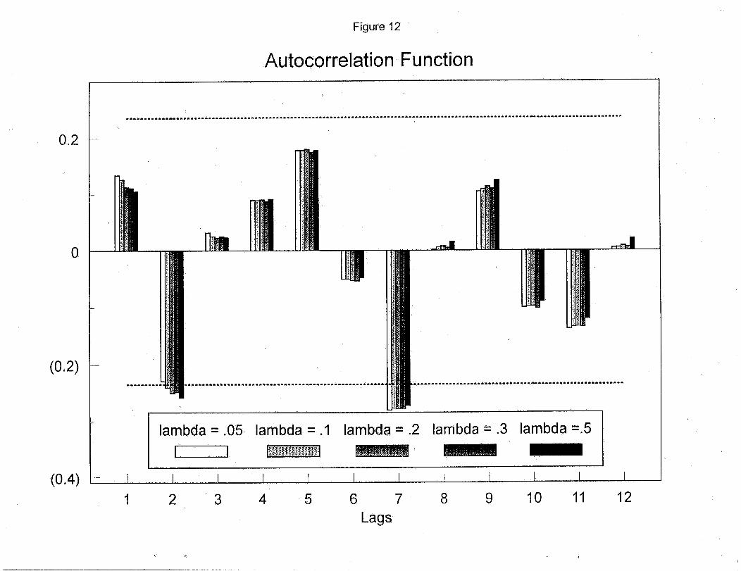
Figure 12

Autocorrelation Function

0.2

0

(0.2)

(0.4) I1

lambda = .05 lambda =.1~

lambda = .2 lambda = .3 lambda =.5

2 3 4 5 6 7 8 9 10Lags

11 12

Figure 13

Rolling Regression Reaction Function Parameter EstimatesWith PEH Consistent Estimates

0.6

0.4

0.2

(0.2)

(0.4)

.........2 Standard Error BandsPEH-I_mplied ,...~ : ..

Inflation Response .......

....¯ .--":",. ........"-"" ............. A....,...-. i~.. ...... -..-"-"-..’k’ .~,,/.-.,~ "-." f--" .~\

Rolling Regression "" " :Estimate ""’"’- .....:-’" :"

0.8......... 2 Standard Error Bands Polling

RegressionEstimate

0.6/ ;

0.20"4 .... .-;’"-" / ............... ""-.

..... ’,. ............... ’..;"’’~v""" ;: "" ..~

PEH-implic~Output Response(o.2~....................... ~2~i ..... ’ ...... ’ ............... ’ ....... ’ ....... ’ ..................................."66Q1 68Q1 70Q1 74Q1 76Q1 78Q1 80Q1 82Q1 84Q1 86Q1 88Q1 90Q1 92Q1

......... 2 Standard Error Bands ,!

1 ii i:~ f Rolling Regression.¯ "i .."

¯ ,, : :.:.: .. ... ~ ::’. : ~.: ::.," ^’.. ... . ; ~" ¯ .....’... ....... :." ......................... . .... ..~ ~ o- -:

.̄,......."~ .." PEH-Impliedt7 Inflation Target .’i:"~ v--,- ~.~ ,

(1)6~! .......

~1 ....... ~ ..... ,,!,, ..... t ....... I~ ..... I, ,,’,,,~ ....... I~li~ .... I ....... t ....... ~,,,

Q1 68Q1 70Q1 72Q1 74Q1 76Q1 78Q1 80Q1 82Q1 84Q1 86Q1 88Q1 90Q1 92Q1

(0.5)

Note: Standard Errors were Iinearly interpolated for 71Q2-Q4, 72Q2-Q3, 77Q2-78Q2, and 81Q2-Q3.