modeling macro-political dynamicspbrandt/patrick_brandts_website/research_files/... · modeling...

doi:10.1093/pan/mpp001

Modeling Macro-Political Dynamics

Patrick T. BrandtSchool of Economic, Political and Policy Sciences, The University of Texas at Dallas

800 W. Campbell Road, GR 31, Richardson, Texas 75080e-mail: [email protected] (corresponding author)

John R. FreemanDepartment of Political Science, University of Minnesota,

1414 Social Science Building, 267 19th Ave. South, Minneapolis, MN 55455e-mail: [email protected]

Analyzing macro-political processes is complicated by four interrelated problems: model

scale, endogeneity, persistence, and specification uncertainty. These problems are endemic

in the study of political economy, public opinion, international relations, and other kinds of

macro-political research. We show how a Bayesian structural time series approach

addresses them. Our illustration is a structurally identified, nine-equation model of the U.S.

political-economic system. It combines key features of the model of Erikson, MacKuen, and

Stimson (2002) of the Americanmacropolity with those of a leading macroeconomic model of

the United States (Sims and Zha, 1998; Leeper, Sims, and Zha, 1996). This Bayesian

structural model, with a loosely informed prior, yields the best performance in terms of model

fit and dynamics. This model 1) confirms existing results about the countercyclical nature of

monetary policy (Williams 1990); 2) reveals informational sources of approval dynamics:

innovations in information variables affect consumer sentiment and approval and the impacts

on consumer sentiment feed-forward into subsequent approval changes; 3) finds that the real

economy does not have any major impacts on key macropolity variables; and 4) concludes,

contrary to Erikson, MacKuen, and Stimson (2002), that macropartisanship does not depend

on the evolution of the real economy in the short or medium term and only very weakly on

informational variables in the long term.

1 Introduction

Many political scientists are interested in modeling macro-political systems. Aggregatepublic opinion research focuses on a small number of opinion variables and some economicvariables. Political economists analyze data on policy and economic outcomes of interest tovoters, outcomes that are functions of underlying political variables. International relationsscholars typically model the behavior of belligerents over time to analyze the evolution ofcooperation and conflict.

Authors’ note:Aprevious version of this paperwas presented at the 2005AnnualMeeting of theAmerican PoliticalScienceAssociation,Washington,DC, and at a seminar at theCollege ofWilliamandMary. The authors thank JanetBox-Steffensmeier, Harold Clarke, Brian Collins, Chetan Dave, Larry Evans, Jeff Gill, Simon Jackman, and RonRappoport for useful feedback and comments. Replication materials, additional appendices, and additional resultsare available on the Political AnalysisWeb site or from P.T.B. The authors are solely responsible for the contents.

! The Author 2009. Published by Oxford University Press on behalf of the Society for Political Methodology.All rights reserved. For Permissions, please email: [email protected]

Political Analysis Advance Access published March 25, 2009

Modeling macro-political dynamics in these varied research areas is complex for fourreasons. The first is the problem of scale. By scale, we mean the number of (potentially)endogenous variables in a model. Macro-political systems are composed of many variablesand of multiple causal relationships. To capture these relationships, several equations areneeded. For instance, in American political economy one must take into account therelationships between public opinion variables and partisanship, and between thesevariables and economic output, employment, and prices. Each relationship requires a sep-arate, dynamic equation. Similarly, students of international relations must account for thebehavioral relationships of all important belligerent groups within and between countries.A separate equation is needed for each directed, dyadic behavior.

A closely related, second problem is endogeneity. Although some variables in macro-political processes clearly are exogenous, we believe that others are both a cause and a con-sequence of each other. For example, our understanding of democracy implies that there issome popular accountability for economic policy and thus endogeneity between popularevaluations of the economy and macroeconomic outcomes (or policies).

Persistence is a third problem. Some variables are driven by short-term forces that canbe exogenous to the macro-political process under study. There also are deeper, medium,and long-term forces that make trends in variables persist and even create long-term, com-mon trends among variables (e.g., cointegration).

Finally, specification uncertainty is a problem.We have no equivalent of macroeconom-ics’ General Equilibrium Theory that can help us specify functional forms. The problems ofscale, endogeneity, and persistence mean that models have many coefficients and that theirdynamic implications (impulse responses) and forecasts havewide error bands (i.e., are quiteimprecise). Because of these problems, our models may also tend to overfit our data.

None of the approaches commonly used to model dynamic processes in political sciencetogether addresses all four problems. The most commonmacro-models are single-equationautoregressive distributed lag (ADL) models and pooled time series cross-sectional(TSCS) regressions. These single-equation models expressly omit multiple relationshipsamong endogenous variables. Common practice is to make each relationship the subjectof a different article (or book chapter). This treats each variable as a dependent in onearticle (chapter) and independent variable in another.1 Users of ADL and TSCS modelsusually acknowledge endogeneity problems, but rarely perform exogeneity tests. Rather adhoc solutions to this problem are used like omitting contemporaneous relationshipsbetween variables, temporally aggregating data, and employing contrived variables for si-multaneity. Some researchers use instrumental variable estimators for this purposebut rarely evaluate the adequacy of their instruments. Also, treatments of persistenceoften are based on knife-edged pretests for unit roots. Perhaps it is not surprising thenthat Wilson and Butler (2007) recently reported that the results of many published articlesthat use single-equation TSCS models are not robust to simple changes in modelspecification.2

1For a recent review of ADL and single-equation models, see De Boef and Keele (2008).2In international political economy it is common to put on the right-hand-side of a single equation explaininga particular policy variable in country i, the average level of the same variable in all other countries (sans i).Franzese and Hays (2005) propose a better approach to TSCS modeling based on spatial statistics. However, theyonly consider endogeneity for one variable. Wilson and Butler (2007) focus on the assumptions macro-politicaltheorists make about unit effects and first-order dynamics in simple single-equation TSCSmodels. They note thatif assumptions of exogeneity also were evaluated along with the possibility of more complex dynamics (longerlag lengths, nonstationarity, etc.), the results reported in many published works are likely to be even less robust(see especially pp. 115–6, 120).

2 Patrick T. Brandt and John R. Freeman

Reduced form (RF) vector autoregression (VAR) representations of simultaneous equa-tion models address these scale and endogeneity issues. Some users of RFs in comparativepolitical economy analyze models with three to four variables (or equations) where allvariables are endogenous. The problem is that most macroeconomists now argue that thereare many more key relationships in markets. Models with more variables are needed tocapture macroeconomic dynamics (e.g., Leeper, Sims, and Zha 1996).We know of noworkin international political economy with a RF model on this scale, for instance, a model thatincludes three to four equations for each of three or four trading partners (cf. Sattler,Freeman, Brandt 2008, 2009).3 Students of international conflict have built RF modelswith 24–28 equations, but restrict their investigations to simple (Granger) causality testing.They do not use their models to study conflict dynamics or to produce forecasts becausewithout some restrictions on the model the specification uncertainty renders the dynamicresponses quite imprecise.4

Finally, users of simulation methods such as Erikson, MacKuen, and Stimson (2002,chap. 10) and Alesina, Londregan, and Rosenthal (1993) address the scale and persistenceissues. But they expressly eschew endogeneity, making restrictions that treat macro-political processes as (quasi-)recursive. Moreover, these researchers often do not producemeaningful measures of precision in their dynamic analyses, for example, no error bandsfor their impulse responses.5

Table 1 summarizes some the models used to address the four problems discussedabove. As we move from VAR models on the left, to Bayesian VAR, and finally to thenew model that is potentially more useful than current macro-political models, in theBayesian Structural Vector Autoregression (B-SVAR) we see that we can address all fourproblems. Part one of the paper explains the nature of the B-SVARmodel, distinguishing itfrom more familiar RF models like frequentist VAR, vector error correction model(VECM), and also BVAR, and explaining how it addresses the four problems listed inTable 1. The rationale for using elucidated, informed priors rather than uninformed or older‘‘Minnesota’’ priors is explained in this part. The criteria used to evaluate the performanceof B-SVARs and of the informed prior in their specifications also is explained here.6

Part two shows how this model can be used to analyze the American macro-politicaleconomy. We construct a nine-equation, structurally identified Bayesian time series modelof the U.S. political-economic system. This model combines key features of the model ofErikson, MacKuen, and Stimson (2002, chap. 10) of the American macropolity with thoseof a leading neo-Keynesian U.S. macroeconomic model (Leeper, Sims, and Zha 1996;Sims and Zha 1998). This structural model, with a loosely informed prior, yields the bestperformance in terms of model fit and dynamics. This loose prior model 1) confirms ex-isting results about the countercyclical nature of monetary policy (Williams 1990), 2) re-veals informational sources of approval dynamics: innovations in information variables

3Franzese (2002) pools time series for countries in a VECM.While simultaneously addressing issues of scale andpersistence, it is not clear how (if) he handles endogeneity within and between countries.4Examples of these larger-scale RF models in international relations are Goldstein and Pevehouse (1997),Pevehouse and Goldstein (1999), and Goldstein et al. (2001).5Erikson,MacKuen, and Stimson (2002, 386) refer to endogeneity as a ‘‘nuisance’’ and a ‘‘nightmare.’’ Their anal-ysis imposes strong restrictions—some contemporaneous relationships are ignored and a recursive structure—onthe interrelationships between variables and on their lag specifications. This is despite their argument that feed-back is a defining feature of the macro-political economy. Erikson, MacKuen, and Stimson also provide no errorbands for their impulse responses.6Our 2006 paper in Political Analysis explained modern BVAR models and how to use them in innovation ac-counting, forecasting, and policy analysis. The focus in the present paper is on B-SVAR models and on the moregeneral problem of modeling and identifying macro-political processes.

3Modeling Macro-Political Dynamics

affect consumer sentiment and approval and the impacts on consumer sentiment feed-forward into subsequent approval changes, 3) finds that the real economy does not haveanymajor impacts on keymacropolity variables, and 4) concludes that, contrary to Erikson,MacKuen, and Stimson (2002), macropartisanship does not depend on the evolution of thereal economy in the short or medium term and only very weakly on informational variablesin the long term. In the spirit of the Bayesian approach (Gill 2004, 2007; Jackman 2004,2008), we believe that these results are insensitive to alternative specifications of priorbeliefs, including beliefs motivated by the late-1990s macropartisanship debate. Directionsfor extending the Bayesian structural time series approach to macro-political analysis andto linking it with formal theory are discussed briefly in the conclusion.

2 Bayesian Time Series Models and the Study of Macro-political Dynamics

Following the publication of Sims (1980) seminal article on macroeconomic modeling,political scientists began exploring the usefulness of RF methods such as VAR (Freeman,Williams, and Lin 1989; Williams 1990; Brandt and Williams 2007). This approach holdsthat macro-theory is not strong enough to specify the functional forms of equations. Macro-theory is at best a set of loose causal claims that translate into a weak set of model re-strictions. Therefore, progress in macro-theory results from analyzing RF models and

Table 1 RF, Bayesian, and structural models of macro-politics

Models

Problems VAR/VECM (RF) BVAR (Bayesian) B-SVAR (Bayesianand structural)

Scale (typical) 4–6 Equations 6–8 Equations 8–18 EquationsEndogeneity Recursive/decomposition

of the endogenousrelationships

Recursive/decompositionof the endogenousrelationships

Theoretically impliedcontemporaneousrelationships that maybe nonrecursive and/oroveridentified

Persistence anddynamics

Pretests for lag length,unit roots, andcointegration

Elucidated informedprior for randomwalks; dummyvariable priors forpersistence andcointegration

Elucidated informedprior for random walks,persistence, andcointegration, conditionalon contemporaneousidentification

Specificationuncertainty

Pretesting; ‘‘Letdata speak’’

Elucidated equation-by-equation prior thatgenerates a nonstandardposterior density

Theoretically informedstructural identificationand yields a system-wideprior with a tractableconditional posteriordensities

Political scienceexamples

Edwards and Wood(1999), Goldsteinet al. (2001)

Williams (1993a),Williams andCollins (1997)

Brandt, Colaresi, andFreeman (2008), Sattler,Freeman, and Brandt (2008)

Econometricreferences

Sims (1972, 1980) Doan, Litterman,and Sims (1984),Litterman (1986)

Leeper, Sims, and Zha(1996), Sims and Zha (1998)


subjecting these models to (orthogonalized) shocks in the respective variables (e.g., inno-vation accounting or impulse responses). If there are any structural implications of theo-ries, they are best represented as contemporaneous relationships between our variables, butthen only as zero restrictions (Bernanke 1986). In the last 20 years, this approach has beenapplied to a wide range of topics in political science such as agenda setting, public opinion,political economy, and international conflict.

A parallel development in political science is the use of the Bayesian methods. Thisapproach rests on two main premises: 1) political phenomena are inherently uncertainand changing and 2) available prior information should be used in model specification(Gill 2004, 324). Bayesianism stresses systematically incorporating previous knowledgeinto the modeling process, being explicit about how prior beliefs influence specificationand results, making rigorous probability statements about quantities of interest, and gaug-ing sensitivity of the results to a model’s assumptions (ibid. 333–4).7

Herewe bring these two developments together.We show how 1) the Bayesian approachmakes time series analysis both more systematic and informative and 2) how prior infor-mation about dynamics and contemporaneous relationships can be utilized.

2.1 Bayesian Structural Vector Autoregessions

We first present a multiple-equation model for the relationships among a set of endogenousvariables. Our goal in employing such a system of equations is to isolate the behavioralinterpretations of the equations for each variable by imposing structure via restrictions onthe system of equations.8 The contemporaneous structure of the system is important for tworeasons. First, it identifies (in a theoretical and statistical sense) these possible contempo-raneous relationships among the variables in the model. Second, restrictions on the struc-tural relationships imply short- and long-term relationships among the variables.

The basic model we propose for macro-political data has one equation for each of theendogenous variables in the system. Each of the endogenous variables is a function of thecontemporaneous (time ‘‘0’’) and p past (lagged) values of all the endogenous variables inthe system. This produces a dynamic simultaneous equation model that can be written inmatrix notation as,

Yt1!m

A0m!m

Xp

‘ 5 1

Yt2‘1!m

A‘m!m

5 d1!m

1 et1!m

t 5 1; 2; . . . ;T; "1#

with each vector’s and matrix’s dimensions noted below the matrix. This is an m-dimen-sional VAR for a sample size of T, with yt a vector of observations for m variables at time t,A‘ the coefficient matrix for the ‘th lag, ‘ 5 1, . . ., p, p the maximum number of lags(assumed known), d a vector of constants, and et a vector of i.i.d. normal structural shockssuch that

7Gill (2004, 333–4) lists seven features of the Bayesian approach. Only four of these are mentioned in the text.Others include updating tomorrow’s priors on the basis of today’s posteriors, treating missing values in the sameway as other elements of models like parameters, and recognizing that population quantities change over time.Jackman (2004) explains how frequentist and Bayesian approaches differ but also how, under certain conditions,their inferences can ‘‘coincide’’ (e.g., when the prior is uniform, the posterior density can have the same shape asthe likelihood). See also Gill (2004, 327–28).8This structure and the equations themselves start from an unrestricted VARmodel. The goal is to impose plausiblerestrictions on the contemporaneous relationships among the variables. Zha (1999) considers restrictions onlagged values of the variables.


E$etjyt2s; s > 0% 5 01!m

; and $e#tetjyt2s; s > 0% 5 Im!m

:

Equation (1) is a structural VAR or SVAR. Two sets of coefficients in it need to bedistinguished. The first are the coefficients for the lagged or past values of each variable,A‘, ‘5 1, . . ., p. These coefficients describe how the dynamics of past values are related tothe current values of each variable. The second are the coefficients for the contempora-neous relationships (the ‘‘structure’’) among the variables, A0. The matrix of A0 coefficientsdescribes how the variables are interrelated to each other in each time period (thus the time‘‘0’’ impact). For example, if the data are monthly, these coefficients describe how changesin each variable within the month are related to one another. Relationships exist outside ofthat month (in the past) are described by the A‘ (lag) coefficients. The contemporaneouscoefficient matrix for the structural model is assumed to be nonsingular and subjects only tolinear restrictions.9 Zero restrictions on elements of A0 imply that the respective variablesare unrelated contemporaneously.

This model is estimated via multivariate regression methods (Sims and Zha 1998;Waggoner and Zha 2003a). The Bayesian version of this model or B-SVAR incorporatesinformed beliefs about the dynamics of the variables. These beliefs are represented ina prior distribution for the parameters. Sims and Zha (1998) suggest that the prior forA‘ is conditioned on the specification decision for A0.

10 To describe the prior, we placethe corresponding elements of A0 and the A‘ into vectors. For a given A0, contemporaneouscoefficient matrix, let a0 be a vector that is the columns of A0 stacked in column-majororder for each equation. For the A‘ parameters that describe the lag dynamics, let A1 be an(m2p1 1)! mmatrix that stacks the lag coefficients and then the constant (rows) for eachequation (columns). Finally, let a1 be a vector that stacks the columns of A1 in columnmajor order (so the first equation’s coefficient, then the second equation’s, etc.). The priorover a0 and a1, denoted p(a) is then,

p!a"5 p

!a0"/!a1;W

"; "2#

where the tilde denotes the mean parameters in the prior density for a1, / (&, &) is a mul-tivariate normal with mean a1 and covariance W.11

Sims and Zha’s (1998) prior for equation 2 addresses the main problems of macro-modeling. For example, the prior addresses the scale problem by putting lower probabilityon the coefficients of the lagged effects, thus shrinking these parameters toward zero. Butrather than imposing (possibly incorrect) exact restrictions on these coefficients such as

9Herewe use theword ‘‘structural’’ to define amodel that is a dynamic simultaneous system of equations with thecontemporaneous relationships identified by the A0 matrix.

10This prior is a revised version of the ‘‘Litterman’’ or ‘‘Minnesota’’ prior for RF VAR models (Litterman 1980;Doan, Litterman, and Sims 1984; Brandt and Freeman 2006). Doan, Litterman, and Sims (1984, 2, 4, respec-tively) originally referred to the Minnesota prior as a ‘‘standardized prior’’ or ‘‘empirical prior’’. Today, em-pirical macroeconomists say the prior is based on their extensive experience in forecasting economic time seriesand ‘‘widely held beliefs’’ about macroeconomic dynamics (e.g., Sims and Zha 1998, fn. 7). In this sense, itresembles the first prior discussed by Jackman (2004). Empirical macro-economists call the Sims-Zha hyper-parameters a ‘‘reference prior.’’ Their use of the term thus is more consistent with convention in their discipline(Zellner and Siow 1980) than in statistics (Bernardo 1979). Finally, such priors also can be elicited (Kadane,Chan, and Wolfson 1996). However, in empirical macroeconomics, the prior almost always is elucidated asa widely held belief. An exercise of this type in political science is Western and Jackman (1994).

11When the prior in equation (2) has a symmetric structure (i.e., it differs by only a scale factor across the equa-tions), the posterior conditional on A0 is multivariate normal. See Kadiyala and Karlsson (1997), Sims and Zha(1999), and Brandt and Freeman (2006).


zeroing out lags or deleting variables altogether, the prior imposes a set of inexact restric-tions on the lag coefficients. These inexact restrictions are prior beliefs that many of thecoefficients in the model—especially those for the higher order lags—have a prior mean ofzero. The prior is then correlated across equations in a way that depends on the contem-poraneous relationships between variables (the covariance of RF disturbances via the A0

matrix of the SVAR). This allows beliefs about the identification of systems such as themacro-political economy to be included a priori and thus improve inferences and fore-casting. Finally, the prior is centered on a random walk model: it is based on the beliefthat most time series are best explained by their most recent values.12

The Sims-Zha prior parameterizes the beliefs about the conditional mean of the coef-ficients of the lagged effects in a1 given a0 in equation (2). Once more, the prior mean isassumed to be that the best predictor of a series tomorrow is its value today. The conditionalprior covariance of the parameters, V(a1ja0) 5 W is more complicated. It is specified toreflect the following beliefs about the series:

1. The standard deviations (SDs) around the first lag coefficients are proportional tothose for the coefficients of all other lags.

2. The weight of each variable’s own lags in explaining its variance is the same as theweights on other variables’ lags in an equation.

3. The SDs of the coefficients of longer lags are proportionately smaller than those ofthe coefficients of earlier lags. Lag coefficients shrink to zero over time and havesmaller variance at higher lags.

4. The SD of the intercept is proportionate to the SD of the residuals for the equation.13

A series of hyperparameters are used to scale the SD of the model coefficients to reflectthese and other beliefs. Table 2 summarizes the hyperparameters in the Sims-Zha prior.14

The key feature of this specification is that the interdependence of beliefs is reflected in theconditioning of the prior on the structural contemporaneous relationships, A0. Beliefs aboutthe parameters are correlated in the same patterns as the RF contemporaneous residuals. Iffor theoretical reasons we expect large correlations in the RF innovations of two variables,the corresponding regressors are similarly correlated at the first lag to reflect this belief andto ensure that the series move in a way that is consistent with their unconditional corre-lations.15

The posterior density for the model parameters is then formed by combining the likeli-hood for equation (1) and the prior:

Pr!A0;A‘; ‘ 5 1; . . . ; p

"}/

!a1; a0

##Y"/!a1;W

"p!a0": "3#

Estimation and sampling from the model’s posterior is via a Gibbs sampler. The maincomplication in the Gibbs sampler is the sampling from the over-identified cases of the

12This does not mean we are assuming the data follow a random walk. Instead, it serves as a benchmark for theprior. If it is inconsistent with the data, the data will produce a posterior that does not reflect this belief.

13The scale of these SDs is determined by a series of univariate AR(p) regressions for each endogenous variable.The hyperparameters then scale the SDs from the AR(p) regressions for the prior.

14Hyperparameters l5 and l6 have to do with beliefs about dynamics. We explain them in the next section of thepaper.

15Sims and Zha (1998, 955) write ‘‘Thus if our prior on [the matrix of structural coefficients for contemporaneousrelationships among the variables] puts high probability on large coefficients on some particular variable j inequation i, then the prior probability on large coefficients on the corresponding variable j at the first lag is high aswell.’’


contemporaneous A0 coefficients. Waggoner and Zha (2003a) show how to properly drawfrom the posterior of A0 given the identification restrictions that may be imposed on the A0

coefficients. We have implemented this Gibbs sampler for the full set of posterior coef-ficients. We employ it here to estimate our B-SVAR model of the American political econ-omy.16

A key feature of the B-SVAR model is that its contemporaneous restrictions affect thedynamic parameters. This can be seen by examining the RF of the structural model inequation (1). The RF representation of the B-SVAR is written in terms of the contempo-raneous values of the (endogenous) variables and their (weakly exogenous or predeter-mined) past values,

yt 5 c 1 yt21B1 1 & & & 1 yt2pBp 1 u t; t 5 1; 2 . . . ; T: "4#

This is anm-dimensional multivariate time series model for each observation in the sample,with yt an 1!m vector of observations at time t, B‘ them!m coefficient matrix for the ‘thlag, and p the maximum number of lags. In this formulation, all the contemporaneouseffects (which are in the A0 matrix of the SVAR) are included in the covariance of theRF residuals, ut.

The RF in equation (4) is derived from the SVAR model by post-multiplying equation(1) by A21

0 . This means that the RF parameters are transformed from the structural equationparameters via

c 5 dA210 ;B‘ 5 2A‘A

210 ; ‘ 5 1; 2; . . . ; p; ut 5 etA21

0 ; "5#

where the last term in equation (5) indicates how linear combinations of structural residualsare embedded in the RF residuals. As equation (5) shows, restricting elements of A0 to bezero restricts the linear combinations that describe the RF dynamics of the system of equa-tions via the resulting restrictions on B‘ and ut.

These restrictions also affect the correlations among the RF residuals. This is becausezero restrictions in A0 affect the interpretation and computation of the variances of the RFresiduals:

Table 2 Hyperparameters of Sims-Zha reference prior

Parameter Range Interpretation

k0 [0,1] Overall scale of the error covariance matrixk1 > 0 SD about A1 (persistence)k2 5 1 Weight of own lag versus other lagsk3 > 0 Lag decayk4 > 0 Scale of SD of interceptk5 > 0 Scale of SD of exogenous variables coefficientsl5 > 0 Sum of autoregressive coefficients componentl6 > 0 Correlation of coefficients/initial condition component

16Distinctive priors could be formulated for each equation, but then a more computationally intensive importancesampling method must be used to characterize the posterior of the model (Sims and Zha 1998). Because theSims-Zha prior applies simultaneously and has a conjugate structure for the entire system of equations, one canexploit the power of a Gibbs sampler.


Var"ut# 5 E$u#t ut% 5 E$"etA210 ##"etA21

0 #% 5 E$"A21#

0 #e#t etA210 % 5 A21#

0 A210 5 R: "6#

In a standard RF analysis, A210 is specified as a just-identified triangular matrix (via a -

Cholesky decomposition of R) so there is a recursive, contemporaneous causal chainamong the equations. A maximum likelihood method can be used to estimate the RF pa-rameters of the model, and from these parameters the elements of the associated A0 can beascertained.17

For SVARs, the A0 is typically nonrecursive and overidentified. Frequentist estimationuses a maximum likelihood estimation for the nonrecursive contemporaneous relationshipsin the parameters of A0 (Bernanke 1986; Sims 1986b; Blanchard and Quah 1989). Thisprocedure uses the RF residual covariance R in equation (6) to obtain estimates of theelements of A0. In either frequentist or Bayesian approaches to estimation, the RF covari-ance R always has [m ! (m1 1)]/2 free parameters. Thus, A0 also can have no more than[m ! (m1 1)]/2 free parameters. Models for which A0 has less than [m ! (m1 1)]/2 freeparameters or, equivalently, more than [m ! (m 1 1)]/2 zero restrictions, are called over-identified.18

Nonrecursive restrictions on A0 amount to two sets of constraints on the model. First,specifying elements of A0 as zero means that the equations and variables corresponding tothe rows and columns of A0 are contemporaneously uncorrelated. Second, since the RFcoefficients B‘, which describe the evolution of the dynamics of the model, are themselvesa function of the structural parameters (and their restrictions) in equation (5), the restric-tions in A0 propagate through the system over time. In other words, the restrictions on thecontemporaneous relationships in the model in A0 have both short-term and long-term ef-fects on the system.

Since A0 and B‘ describe the RF dynamics of the system, the B-SVAR restrictions alsoaffect the estimates of the impulse responses which are the moving average representationof the impact of shocks to the model. These responses, Ct1s describe how the system reactsin period t1 s to a change in the RF residual us at time s > t. These impulse responses arecomputed recursively from the RF coefficients and A0:

@yt 1 s

@us5 Cs 5 B1Cs21 1 B2Cs22 1 & & & 1 BpCs2p; "7#

with C0 5 A210 and Bj 5 0 for j > p. Since these impulse are functions of the RF coef-

ficients B‘, and B‘ 5 2A‘A210 , the structural restrictions in A0 are present in the dynamics

of the RF of the model.The interpretation of the impulse responses for SVARmodels differs from those of RF

VAR models. In the latter one typically employs a Cholesky decomposition of the Rmatrix, which is a just identified, recursive model. In this case, all the shocks hittingthe system have the same (positive) sign and enter the equations, but according tothe ordering of the variables in the Cholesky decomposition. Systems with a Cholesky

17The RF maximum likelihood case, where A210 is a Cholesky decomposition of R, implies a recursive or Wold

causal chain between the disturbances. This Cholesky decomposition exists because the RF error covariancematrix R is positive definite. For a discussion and application of the concept of a Wold causal chain in politicalscience, see Freeman, Williams, and Lin (1989) or Brandt and Williams (2007).

18To estimate nonrecursiveA0’s, it is necessary to satisfy both an order and a rank condition as detailed in Hamilton(1994, 1994, section 11.6). (Note that as regards Hamilton’s formulation, in our case his D matrix is an identitymatrix.) In our illustration below, the numerical optimization of the posterior peak requires that the rankcondition is satisfied.


decomposition have a triangular structure where the shocks make each left-hand-sidevariable in the system move in a positive direction. With the Cholesky, decompositionshocks in equations are uniquely related to shocks in variables. In an SVAR system, be-cause there are no unique left-hand-side variables, there is no unique correspondencebetween shocks in variables and shocks to equations. Thus, shocks to a given equationcan be positive or negative as a result. One could normalize the shocks to be a particularsign, but this is merely selecting among the modes of the posterior of the coefficients inA0. This ‘‘sign normalization’’ complicates the sampling of the model but leaves the in-terpretation of the orthogonal shocks in the SVAR unchanged for the respective impulseresponses.19

2.2 Modeling Macro-Political Dynamics

This B-SVAR model is quite general and it subsumes a number of well-known mod-els as special cases: ADL models, error correction models, ARIMA models, RF andsimultaneous equation models, etc. (for details, see Brandt and Williams 2007).This generality allows us to address the four main problems of macro-modeling outlinedearlier.

Complexity and Model Scale: Modeling politics as a system requires an analyst to spec-ify a set of state variables and the causal connections between them.20 The problem is thatas more variables are needed to describe a system, the usefulness of the model diminishes.The model proposed in equation (1) for m variables can have m2p 1 m estimable coef-ficients in A1 and up to [m ! (m 1 1)]/2 coefficients in A0. This is a large number ofparameters—even for small choices of m and p (if m 5 6 and p 5 6, this would be237 parameters). The flexibility of the model comes at a cost: higher degrees of parameteruncertainty relative to the available degrees of freedom.21

The results of this cost are that inferences tend to be rather imprecise. So efforts to assessthe impact of political and economic variables on each other may produce null findingsbecause of a lack of degrees of freedom relative to the number of parameters. These prob-lems arise because large, unrestricted models tend to overfit data. For example, they at-tribute too much impact to the parameters on distant lags.22 One solution is to restrict thenumber of endogenous variables in the model and to restrict the dynamics by limiting thenumber of lagged values in the model. As noted in the Introduction, political scientists whostudy macro-political dynamics are comfortable with the concept of a (sub)system whetherin terms of the macropolity (Erikson, MacKuen, and Stimson 2002) or international con-flict (Goldstein et al. 2001). But these restrictions are problematic because they are oftenad hoc and can lead to serious inferential problems (Sims 1980).

19For discussion of the implications of sign normalization, seeWaggoner and Zha (2003a). This is discussed belowin the interpretation of our illustration. It also surfaces in applications of the B-SVAR model to the Israeli-Palestinian conflict (Brandt, Colaresi, and Freeman 2008).

20A system is a ‘‘particular segment of historically observable reality [that] is mutually interdependent and ex-ternally, to some extent, autonomous’’ (Cortes, Przeworski, and Sprague, 1974, 6). And the state of a dynamicsystem, as embodied in a collection of state variables, is ‘‘the smallest set of numbers which must be specified atsome [initial time] to predict uniquely the behavior of the system in the future’’ (Ogata 1967, 4).

21A contrast to this is item-response theory models that are used to model ideological scales. There the number ofparameters is large and helps in fitting the model of multiple responses.

22Sampling error tends to cause the standard errors on distant lag coefficients to be underestimated. For more onthe problems associated with increases in model scale relative to the dynamic analysis and forecasting see, Simsand Zha (1998, 958–60), Zha (1998), and Robertson and Tallman (1999, especially, p. 6 and fn. 7).


Using the Sims-Zha prior in a structural VARmodel has two distinct advantages. First, itallows us to work with larger systems with a set of informed or baseline inexact restrictionson the parameters. Second, it reduces the high degree of inferential uncertainty producedby the large number of parameters. For instance, the Sims-Zha prior produces smaller andsmaller variances of the higher order lags (via k3).

Endogeneity and Identification: Political scientists are aware of the problem of simul-taneity bias. They also are sensitive to the fact that their instruments may not be adequate toeliminate this bias (Bartels 1991). But when it comes to medium- and large-scale systems,most political scientists are content to make strong assumptions about the exogeneity ofa collection of ‘‘independent variables’’ and to impose exact (zero) restrictions on the co-efficients of lags of their variables. In cases like the work of Erikson, MacKuen, andStimson on the American macropolity (2002, chap. 10), an entire, recursive equationsystems is assumed.23

The deeper problem here is that of identification or structure. In the case of macro-political analysis, this problem is especially severe because we usually work in nonexper-imental settings. Manipulation of variables and experimental controls is not possible.Manski (1995, 3) emphasizes the seriousness of this problem: ‘‘. . . the study of identifi-cation comes first. Negative identification findings imply that statistical inference isfruitless . . ..’’ Manski acknowledges endogeneity as one of three effects that make iden-tification difficult.24

Structure in a B-SVAR model amounts to the contemporaneous relationships betweenthe variables that one expects to see. Those that are not plausible are restricted to zero (sozeros are placed in appropriate elements of the contemporaneous coefficient matrix A0) andthe remaining contemporaneous relationships are estimated. The real advantages of thismodeling approach are as follows: 1) it forces analysts to confront and justify which re-lationships are present contemporaneously and 2) it imposes restrictions on the paths of therelationships over time. This is particularly relevant in political economy applications.Consider, for instance, a model of monetary policy and presidential approval. Here, eco-nomic variables affect monetary policy making and vice versa. Hence, the structural spec-ification has to include economic as well as political relationships. Just as critical isspecifying the timing of the impacts of relationships among approval, monetary policy,and the economy (e.g., see Williams (1990)). Some of the variables are likely to be con-temporaneously related—for example, approval and monetary policy.

To specify the contemporaneous structure of the B-SVARmodel, the equations in thesystem often are partitioned into groups called ‘‘sectors.’’ These sectors are linear com-binations of the contemporaneous innovations as specified in the A0 matrix. These sec-tors of variables then are ordered in terms of the speed with which the variables in themrespond to the shocks in variables in other sectors. In macroeconomics, some aggregateslike output and prices are assumed to respond only with a delay to monetary and other kindsof policy innovations. Restrictions on these contemporaneous relationships therefore implythat the economic output variables are not contemporaneously related to monetary policy.Competing identifications are tested by embedding their implied restrictions on contem-poraneous relationships in a larger set of such restrictions and assessing the posterior den-sity of the data with respect to the different identifications. The overidentified and

23Erikson, MacKuen, and Stimson do perform a handful of exogeneity tests. See, for instance, the construction oftheir presidential approval model. But when it comes to analyzing their whole system, they simply posit a re-cursion for their ‘‘historical structural simulation.’’ We elaborate on this point in our illustration.

24The other two effects that confound identification are contextual effects and correlation effects.


nonrecursive nature of the A0 matrix create challenges in estimation and interpretation ofthe model.25

Persistence and Dynamics: Political series exhibit complex dynamics. In some cases, theyare highly autoregressive and equilibrate to a unique, constant level. In other cases, the seriestend to remember politically relevant shocks for very long periods of time thus exhibitingnonstationarity (i.e., a stochastic trend). In still other cases, these stochastic political trends tendtomove together and are thus cointegrated. Political scientists have found evidence of stochastictrends in approval and uncovered evidence that political series are (near) cointegrated (e.g.,Ostrom and Smith 1993; Clarke and Stewart 1995; Box-Steffensmeier and Smith 1996;De Boef and Granato 1997; Clarke, Ho and Stewart 2000). Erikson, MacKuen, andStimson (1998, 2002, chap. 4) make a sophisticated argument about the interpretation ofmacropartisanship as a nonstationary ‘‘running tally of events.’’ Such arguments revealthese scholars’ beliefs about whether a series will re-equilibrate. How quickly this occursand the implications for inference are matters of debate.

Our point is that these beliefs are best expressed as probabilistic statements rather thanbased on knife-edged tests for cointegration or unit roots. One of the benefits of usinga Bayesian structural time series model is that it allows us to investigate beliefs aboutthe dynamic structure of the data. If the researcher has a strong belief about the stationar-ity/nonstationarity of the variables, one can combine this belief with the data and see if itgenerates a high- or low-probability posterior value (rather than a knife-edged result).

The Sims-Zha prior accounts for these dynamic properties of the data in three ways. Thefirst is by allowing the prior beliefs about SD around the first lag coefficients k1 to be small,implying strong beliefs that the variables in the system follow random walks and are non-stationary.26 The prior allows analysts to incorporate beliefs about stochastic trends andcointegration. Continuing with the enumeration in Table 2, the Sims-Zha prior alsoincludes two additional hyperparameters that scale a set of dummy observations orpre-sample information that correspond to the following beliefs:

1. Sum of autoregressive coefficients component (l5): This hyperparameter weights theprecision of the belief that average lagged value of a variable i better predicts variablei than the averaged lagged values of a variable i 6' j. Larger values of l5 correspond tohigher precision (smaller variance) about this belief. This allows for correlationamong the coefficients for variable i in equation i, reflecting the belief that theremay be as many unit roots as endogenous variables for sufficiently large l5.

2. Correlation of coefficients/initial condition component (l6): The level and varianceof variables in the system should be proportionate to their means. If this parameteris greater than zero, one believes that the precision of the coefficients in the modelis proportionate to the sample correlation of the variables. For trending series,the precision of this belief should depend on the variance of the pre-sample meansof the variables in the model and the possibility of common trends among thevariables.

25The idea that theories imply restrictions on contemporaneous relationships may seem new. But Leeper, Sims,and Zha (1996, 9 ff.) point out that such restrictions are implicit in our decisions to make variables predeterminedand exogenous. In terms of the actual estimation, an unrestricted element in A0 means the data potentially canpull the posterior mode for the respective parameter off its prior (zero) value. In contrast, a zero restriction on anelement of A0 forces the respective posterior mode of that element to be zero.

26In the case of stationary data, a ‘‘tight’’ or small value for k1 implies a slow return to the equilibrium value of theseries. A tight value of k4 is a belief in smaller variance around the equilibrium.


Values of zero for each of these parameters imply that both beliefs are implausible.These beliefs are incorporated into the estimation of the B-SVAR using a set of dummyobservations in the data matrix for the model. These dummy observations represent sto-chastic restrictions on the coefficients consistent with the mixed estimation method ofTheil (1963). As l5/N, the model becomes equivalent to one where the endogenousvariables are best described in terms of their first differences and there is no cointegration.As Sims and Zha explain, because the respective dummy observations have zeros in theplace for the constant, the sums of coefficient prior allows for nonzero constant terms or‘‘linearly trending drift.’’ As l6/N, the prior places more weight on a model with a singlecommon trend representation and intercepts close to zero (Robertson and Tallman 1999, 10and Sims and Zha 1998, section 4.1).

The possibility of nonstationarity makes Bayesian time series distinctive from otherBayesian analyses. In the presence of nonstationarity, the equivalence between Bayesianand frequentist inference need not apply: ‘‘time series modeling is . . . a rare instance inwhich Bayesian posterior probabilities and classical confidence intervals can be in sub-stantial conflict’’ (Sims and Zha 1995, 2). Further, including these final two hyperpara-meters and their dummy observations has a number of advantages. First, it means theanalyst need not perform any pre-tests that could produce mistaken inferences aboutthe trend properties of her or his data. Instead, one should analyze the posterior probabilityof the model to see if the fit is a function of the choice of these hyperparameters.27 Second,claims about near- and fractional integration can be expressed in terms of l5 and l6. Usingthese two additional hyperparameters should enhance the performance of macro-politicalmodels, especially of models of the macro-political economy.28 Finally, the inference prob-lems associated with frequentist models of integrated and near-integrated time series areavoided in this approach. Strong assumptions about the true values of parameters areavoided by the use of Bayesian inference and by sampling from the respective posteriorto construct credible intervals rather than by invoking asymptotic approximations for con-fidence intervals.29

Model Uncertainty: The problem of model uncertainty is an outgrowth of the weaknessof macro-political theory. This uncertainty operates at two levels: theoretical uncertaintyand statistical uncertainty. Theoretical uncertainty includes the specification of the model,such things as endogenous relationships. Statistical uncertainty encompasses the uncer-tainty about the estimated parameters. The uncertainty of these estimates depends onthe prior beliefs, the data, and the structure of the model—which itself may be due to in-determinate theoretical structure.

27Information about the probability of unit roots and cointegration vectors can be computed from a posteriorsample. We could compute lag polynomials for each draw and then look at the implied stationarity and cointe-gration to get a summary measure of the behavior around the unit circle. In these cases, one might want a priorover such behavior, such as that suggested by Richard (1977). This would be another alternative to the priorssuggested in footnote 10.

28Robertson and Tallman (1999, 2001) compare the forecasting performance of a wide number of VAR and Bayes-ian VAR specifications. They find that it is the provision for unit roots and common trends that is most respon-sible for the improvement in the forecasting performance of their model over unrestricted VARs and over VARswith exact restrictions.

29From the Bayesian perspective, nonstationarity is not a nuisance. Williams (1993b) and Freeman et al. (1998)document the problems nonstationarity causes for political inference. The crux of the problem is whether thetrue values of parameters are in a neighborhood that implies nonstationarity. If they are, in finite samples, normalapproximations may be inaccurate as the boundary of the region for stationary parameters is approached. Em-pirical macroeconomists are reluctant, as we should be, to assume that parameters are distant from this boundary(see Sims and Zha 1995, 2). This problem seems to be overlooked by our leading Bayesians Gill (2004, 328) andJackman (2004, 486).


Observational equivalence (viz., poor identification) is a consequence of both forms ofuncertainities, which are often hard to separate. Too often multiple models explain the dataequally well. As the scale of our models increases, this problem becomes more and moresevere: models with many variables and multiple equations will all fit the data well (Leeper,Sims, and Zha 1996, 14–15; Sims and Zha 1998, 958–60). Models that are highly param-eterized and based on uncertain specifications complicate dynamic predictions. The degreeof uncertainty about the dynamic (impulse) responses of medium- and large-scale systemsinherits the serial correlation that is part of the endogenous systems of equations. Hence,conventional methods for constructing error bands around them are inadequate (Sims andZha 1999).30

How then do we select from among competing theoretical and statistical specifications?We first need to be able to evaluate distinct model specifications or parametric restrictions(e.g., specifications based on different theoretical models, restrictions on lag length, equa-tions, A0 identification choices). Second, there are a large variety of possible prior beliefsfor BVAR and B-SVAR models.

Evaluationsofmodelspecificationsarehypothesistestsandaretypicallyevaluatedusingsomecomparison of a model’s posterior probability—such as Bayes factors where one compares theprior odds of two (or more) models to the posterior odds of the models. This is appropriate forcomparing functional and parametric specifications. Methods that are particularly relevant for(possibly) non-nested and high-dimensional models like the B-SVAR model are model moni-toring and summaries of the posterior probabilities of various model quantities (see Gill2004). These Bayesian fit measures allow us to analyze the hypotheses about specificationand othermodel featureswithout the necessity of nestingmodels thatmay be consistentwithvarious theories. One thus easily can compare models on a probabilistic basis.

The evaluation of competing prior specifications or beliefs requires comparing differentpriors and their impacts on posterior distributions of the parameters. This is harder to do,since it is a form of sensitivity analysis to see how the posterior parameters (or hypothesistests, or other quantities of interest) vary as a function of the prior beliefs. For large-scalemodels such as B-SVARs, examining the posterior distribution of the large number of in-dividual parameters is infeasible. Although one might desire an omnibus fit statistic such asan R2 or sum of squared error, such quantities will be multivariate and hard to interpret.

One common suggestion by non-Bayesians is to ‘‘estimate’’ the prior hyperparameters.That is, one should treat the hyperparameters as a set of additional nuisance parameters(e.g., fixed effects) that can be estimated as part of the maximization of the likelihood(posterior) of the model. This is problematic, as Carlin and Louis (2000, 31–2) note:‘‘Strictly speaking, empirical estimation of the prior is a violation of Bayesian philosophy:the subsequent prior-to-posterior updating . . . would ‘use the data twice’ (first in the prior,and again in the likelihood). The resulting inferences would thus be ‘overconfident’.’’

Further complicating the assessment of prior specification is the nature of time seriesdata itself. Time series data are not a ‘‘repeated’’ sample. This is what causes many of themajor inferential problems in classical time series analysis, especially unit root analysis.Williams (1993b, 231) argues that ‘‘Classical inference is . . . based on inferring somethingabout a population from a sample of data. In time-series [sic], the sample is not random,and the population contains the future as well as past.’’ The presence of unit roots and the

30A notable exception here is the item-response models used to create ideological scales for members of Congressand Supreme Court justices (Poole and Rosenthal 1997; Poole 1998; Martin and Quinn 2002). Here adding moreparameters actually helps reduce the uncertainty about the underlying ideological indices.


special nature of a time series sample therefore argue against ‘‘testing’’ for the prior. In-stead, priors should reflect our beliefs based on past analyses, history, and expectationsabout the future. They should not then be estimated from the data, as this is only one re-alization of the data generation process.

In practice, two tools are used to evaluate the structural representation of contempo-raneous relationships, A0, and the priors for the B-SVAR model. The first is the log mar-ginal data density (also known as the log marginal likelihood):

log"m"Y## 5 log"Pr"YjA0;A1## 1 log"Pr"A0;A1## ( log"Pr"A0;A1 jY##; "8#

where log(Pr(YjA0,A1)) is the log likelihoodof theB-SVARmodel, log(Pr(A0,A1)) is the logprior probability of the parameters, and log(Pr(A0, A1jY)) is the posterior probability of theB-SVARmodel parameters. Since aGibbs sampler is used to sample theB-SVARmodel, wecan compute the log marginal data density (log(m(Y)) in equation 8 using the method pro-posed by Chib (1995).31 These log probabilities of the data, conditional on the model, sum-marize the probability of the model; they can be computed from the Gibbs sample output(Geweke 2005, chap. 8). Bayes factors can be formed from the logmarginal data densities togauge the relative odds of competing, theoretical representations of contemporaneous po-litical relationships.Again, impluse response analysis is an important complement here. Thestudy of the dynamics of a given structural specification—whether it produces theoreticallymeaningful and empirically sensible impulse responses—is an integral part of the modelevaluation process. Brandt, Colaresi, and Freeman (2008) and Sattler, Freeman, Brandt(2008, 2009) show how to use the log marginal density and impulse responses togetherto evaluate competing structural specifications of important relationships in internationalrelations and comparative political economy.

The same tools are used to evaluate competing priors for B-SVAR models but with twoimportant caveats. The log marginal data density is only applicable for informative priors.Diffuse or improper prior should not be evaluated with this tool. This is because undera diffuse prior, the posterior parameters will have low probability and the in-sample fitwill be too good; an inflated estimate of the log marginal data density will be obtained.32

Also, the impulse responses for diffuse priors almost always are of little use. This is be-cause the scale of these models (in the absence of an informative prior) renders their errorbands too large to allow for any meaningful inferences about the causal effects of shocks inone variable on another. The reason for this is that the diffuse prior allows the sampler tosearch too large a parameter space producing estimates that allow for behavior too far fromthe sample of interest. This is illustrated in the Appendix.

31The quantity estimated for each draw is log"m"Y## 5 log"Pr"YjA0;A1##1log"Pr"A0;A1##2Pm

i 5 1

log"Pr"A0"i#;A1jY; i 6' j##, where m is the number of equations, and A0(i) is the ith column of A0. Note that wedo this computation one column at a time for A0 per the blocking scheme for computing the log marginal densityusing the Gibbs sampler (Chib 1995; Waggoner and Zha 2003a).

32Chib (1995) notes that the quantity in equation 8 is the log of the basic marginal likelihood identity, or

m"Y# 5 Pr"YjA0;A1 #Pr"A0;A1 #Pr"A0;A1 jY#

:

For the diffuse prior model, the posterior probability of the parameters in the denominator of this expression,Pr(A0, A1jY) will be small. This will inflate the value for m(Y) and hence also its logarithm. Kass and Raftery(1995) warn against using diffuse priors in Bayes factor calculations. Among their points is ‘‘. . . using a priorwith a very large spread . . . under [the alternative hypothesis] in an effort to make it ‘noninformative’ will forcethe Bayes factor to favor [the null]. This was noted by Bartlett (1957) and is sometimes called ‘Bartlett’s par-adox.’ As Jeffrey’s recognized, to avoid this difficulty, priors on parameters being tested . . . generally must beproper and not have too big a spread.’’ (ibid. 782).


B-SVARs as an approach to modeling macro-politics: B-SVARmodeling presents somechallenges for political scientists. First, unlike the case for VAR/VECM models, we mustelucidate informed priors that represent the beliefs of the macro-political theorists workingon a particular problem. These beliefs must be translated into the hyperparameters de-scribed above and the sensitivity of model performance to these translations must beassessed. In contrast to BVAR modeling, B-SVAR modeling also requires us to make the-oretically informed specification decisions about the existence of contemporaneous rela-tionships among our variables. To specify the A0 matrix in the model, we must study andtranslate theory into an appropriate set of identifying restrictions. In overidentified cases,some computational problems have to be solved.33

If these challenges can be met, we will have valuable new tools for macro-political anal-ysis. With these tools, we will be able to analyze political systems of medium scale in newways—ways that allow for endogeneity butwhich also incorporate theory and allow tests ofinsights about the contemporaneous relationships between our variables. In addition, we canavoid the inferential pitfalls of pre-testing used in frequentist time series analysis, such asknife-edge decisions about dynamics. Finally, with B-SVAR model, we still will be able tomake meaningful assessments of model performance yet avoid overfitting our data.

The next section turns to an illustration of these virtues of B-SVAR modeling.

3 A B-SVAR Model of the American Political Economy

Modeling the connections between the economy and political opinions has been a majorresearch agenda inAmerican politics. Amajor contribution to this endeavor is the aggregateanalysis of the economy and polity by Erikson, MacKuen, and Stimson (2002, chap. 10)(hereafter, EMS). EMS construct a recursivemodel where economic factors are used to pre-dict political outcomes (e.g., presidential approval and macropartisanship). Their model il-luminates linkages between key economic and political variables. Themodel built here is inthe spirit of their work.We showhow aB-SVARmodel helps us copewith the four problemsdiscussed above and thereby significantly enhances our ability to analyze American macro-political dynamics.34

3.1 The Macro-political Economy in Terms of a Bayesian-SVAR Model

We construct a nine-equation system that incorporates the major features of research aboutthe U.S. macroeconomy and polity. We take as our starting point two parallel bodies ofwork: 1) the macropolity model of EMS and 2) the empirical macroeconomic models inSims and Zha (1998) and Leeper, Sims, and Zha (1996) (hereafter abbreviated as SZ andLSZ, respectively). EMS create a large-scale dynamic model of the polity—how presiden-tial performance, evaluations of the economy and partisanship are related to politicalchoice. We build upon their models and measures to construct a model of the ‘‘political

33Of course, some may be opposed to the use of informed priors. But many researchers also are proponents of theiruse (Gill 2007; Garthwaite, Kadane, and O’Hagan 2005). As we have noted, the use of informed, elucidatedpriors now a standard practice in major branch of empirical macroeconomics.

34Chapter 10 of The Macropolity is a very serious modeling effort. The first part stresses (verbally) and presentsschematically political-economic feedback and endogeneity. But the actual modeling—‘‘historical simulation’’—is mainly computational. To avoid the ‘‘nightmare of endogeneity,’’ EMS use lags and impose a recursivestructure on their system and then place coefficient values from their single-equation estimations into theirequations one-by-one. EMS do not attempt to estimate their whole system of equations simultaneously and,as they themselves note, they do not provide any measures of precision for their impulse responses or forecasts.There is a report of an exogeneity test (123, fn. 8). But most of the identifying restrictions for EMS’s model areposited, but not established through any analyses of the data.


sector’’ of the macro-political economy. The political sector of the model consists of threeequations: macropartisanship (MP), presidential approval (PA), and consumer sentiment(CS).35 Since PA and CS are in large part the result of economic evaluations, the dynamicsof the macroeconomy figure prominently in EMS’s analysis. The feedback from thesepolitical variables to the economy connotes democratic accountability; it involvescausal chains between economic and political variables. Thus, politics is both a causeand a consequence of economics.36 To model the objective economic factors and policythat citizens evaluate, we utilize the empirical neo-Keynesian macroeconomic model of SZand LSZ. We incorporate the economy by adding to the three variable political sectora common six-equation model frequently used by macroeconomic policy makers in theUnited States (inter alia Sims 1986a; Leeper, Sims, and Zha 1996; Sims and Zha1998; Robertson and Tallman 2001). These six economic variables are grouped into foureconomic sectors. The first is production which consists of the unemployment rate (U),consumer prices (CPI), and real GDP (Y). The second and third are a monetary policyand money supply sectors consisting of the Federal funds rate (R) and monetary policy(aggregate M2). The fourth is an information or auction market sector that is theCommodity Research Bureau’s price index for raw industrial commodities (Pcom).37

The interest rate, approval, and MP variables are all expressed in proportions, whereasthe other variables are in natural logarithms.38 All the variables are monthly from January1978 until June 2004.39

These nine endogenous variables—the six economic variables plus CS, PA, andMP—are modeled with a B-SVAR. Our model includes 13 lags. Our model also includesthree exogenous covariates in each of the nine equations. The first is a dummy variable forpresidential term changes, coded 1 in the first three months of a new president’s term ofoffice. The second is a presidential party variable that is coded – 15 Republican, 15 Dem-ocrat. This variable allows us to account for the different effects of economics and politicsacross administrations. This achieves the same effect in our model as the ‘‘mean centering’’of the CS and PA variables in Green, Palmquist, and Schickler (1998).40 The final

35PA and MP marginals are from Gallup surveys obtained from the Roper Center and iPoll; missing values forsome months are linearly interpolated. CS is based on University of Michigan surveys as compiled in FederalReserve Economic Data Base at the St Louis Federal Reserve Bank (http://research.stlouisfed.org/fred2/).

36See the concluding chapter of The Macropolity, especially pages 444–8. EMS quote the arguments of Alesinaand Rosenthal (1995, 224) that ‘‘the interconnections between politics and economics is sufficiently strong thatthe study of capitalist economies cannot be solely the study of market forces.’’ EMS admit, however, that in mostof their book they treat the economy as exogenous to the polity.

37Data on most economic variables and CS were obtained from the Federal Reserve Economic Data Base at the StLouis Federal Reserve Bank (http://research.stlouisfed.org/fred2/). All values are seasonally adjusted whereapplicable. The price index for raw commodities is from Commodity Research Bureau (http://www.crbtrader.-com/crbindex/). The monthly real GDP series was generated using the Denton method to distribute the quarterlyreal GDP totals over the intervening months using monthly measures of industrial production, civilian employ-ment, real retail sales, personal consumption expenditures, and the Institute of Supply Managers’ index ofmanufacturing production as instruments (Leeper, Sims, and Zha 1996).

38The reason for these transformations is that our subsequent dynamic responses for the logged variables and theproportions (when multiplied by 100) will all be interpretable in percentage terms for each variable.

39Note that our sample differs from that used in EMS in twoways. First, we cover a more recent time span than thatused in their analyses since we include data from 1978 to 2004. Second, we are working with monthly data,which means our analysis will contain more sampling variability than the aggregated quarterly data used byEMS to predict the relationships between unemployment, PA, and MP. We use monthly data because their argu-ments imply different reaction times for approval and MP to changes in the economy and CS.

40Including a signed dummy variable for party control in the model is equivalent to signing or estimating party-specific indicators of CS and PA in the model.


exogenous variable is an election counter that runs from 1 to 48 over a four-year presi-dential term. It captures election cycle effects, as suggested by Williams (1990).41

There are two steps to specify a B-SVAR model of the U.S. political economy. The firstis to identify the contemporaneous relationships among the variables. The second is tochoose values for the hyperparameters that reflect generally accepted beliefs about thedynamics of the American political economy. Because the conclusions about political-economic dynamics may be due to these hyperparameters, we analyze the sensitivityof our results to these choices.

The structure of the contemporaneous relationships that we use—the identification ofthe A0 matrix—is presented in Table 3. (The matrix A1 allows for all variables to interactvia lags.) The rows of the A0 matrix represent the sectors or equations, and the columns arethe innovations that contemporaneously enter each equation. The nonempty cells (markedwith X’s) are contemporaneous structural relationships to be estimated, whereas the emptycells are constrained to be zero.

We must provide a theoretical rationale for the contemporaneous restrictions and rela-tionships. Beginning with the economic sectors, the restrictions for the Information, Mon-etary Policy, Money Supply, and Production sectors come from the aforementioned studiesin macroeconomics. This specification of the structure of the economy has been found to beparticularly useful in the study of economic policy (see e.g., Sims 1986b; Williams 1990;Robertson and Tallman 2001;Waggoner and Zha 2003a).42 Next we ask, ‘‘which economicequations are affected contemporaneously by shocks to the political variables?’’ This isa question about the restrictions to the political shocks in the economic equations (theshocks in the three right-most columns and first six rows of Table 3). To allow for politicalaccountability, contemporaneous effects are specified for political variables in two of theeconomic equations. First, the macropolity variables—PA, CS, andMP can have a contem-poraneous effect on commodity prices.43 This is consistent with recent results in interna-tional political economy such as Bernhard and Leblang (2006). Second, PA is expected to

Table 3 General framework for contemporaneous relationships in the U.S. political economy

Sector Variables Pcom M2 R Y CPI U CS PA MP

Information Pcom X X X X X X X X XMonetary policy M2 X X XMoney supply R X X X X XProduction Y XProduction CPI X XProduction U X X XMacropolity CS X X X XMacropolity PA X X X X XMacropolity MP X X X X X X

Note. The X’s (empty cells) represent contemporaneous relationships to be estimated (restricted to zero) in theBayesian SVAR model.

41The second dummy, for party control, may be weakly endogenous. Future research on the model will try to testfor this possibility.

42The distinction between contemporaneous and lagged effects is conceived in terms of the speed of response. Forexample, consider shocks in interest rates. Commodity prices respond immediately to these shocks, whereas ittakes at least a month for firms to adjust their spending to the rise in interest rates. Hence, there is a zero re-striction for the impact of R on Y. Again, there is a lagged effect of R on Y and this is captured by A1.

43We thank an earlier reviewer for suggesting the endogenous relationship betweenMP and the information sector.


have a contemporaneous effect on interest rates and on the reaction of the Federal Reserve(Beck 1987; Williams 1990, Morris 2000). The argument for estimating these structuralparameters is that there can be a within-month reaction by the Federal Reserve to changesin the standing of the presidents who manage their approval. Finally, we ask ‘‘how doeconomic shocks contemporaneously affect the political variables?’’ This is a questionabout the structure of the last three rows of Table 3. We argue that the real economic var-iables—represented by GDP, unemployment, and inflation variables—contemporaneouslyaffect the macropolity. The contemporaneous specification of A0 for the macropolity var-iables (the last three rows of Table 3) allows all the production sector variables to con-temporaneously affect the macropolity variables: innovations in GDP, unemployment,and prices have an immediate effect on CS, PA, and MP. These contemporaneous relation-ships are suggested by the control variables used in EMS and by related studies of theeconomic determinants of public opinion (inter alia, Clarke and Stewart 1995; Green,Palmquist, and Schickler 1998; Clarke, Ho and Stewart 2000). We also specify a recursivecontemporaneous relationship among the CS, PA, and MP variables. This is suggested bythe discussion of purging the economic effects from these variables in EMS (1998). Theblank cells in Table 2 denote the absence of any contemporaneous impact of the columnvariables on the row variables. Finally, note that R has (9! 10)/25 45 free parameters andthe A0 matrix in Table 3 has 38 free parameters. Hence, it A0 is overidentified.

44

ThesecondstepinspecifyingtheB-SVARmodelistorepresent thebeliefsabout themodel’sparameters. These beliefs are specified by the hyperparameters. EMS and SZ reveal similarbeliefs about the character of the macro-political economy. SZ propose a benchmark priorfor empirical macroeconomics with values of k1 5 0.1, k3 5 1, k4 5 0.1, k5 5 0.07, andl55l65 5. These values imply amodelwith relatively strong prior beliefs about unit roots,some cointegration, but with little drift in the variables. This prior corresponds to a politicaleconomy with strong stochastic trends and that is difference stationary. This is very similarto EMS’s ‘‘running tally’’ model that also has stochastic trends but limited drift in the var-iables. EMS also reveal a belief that some variables in their political-economic systemare cointegrated. Illustrative is EMS’s argument that MP is integrated order 1. This revealsa belief the coefficients for the first own lags of some variables should be unity or that k1 issmall. EMS also express confidence that PA andCS do not have unit roots, which is still pos-siblewith these beliefs. We denote this prior by the name ‘‘EMS-SZ Tight’’, or a Tight prior.

Because these hyperparameters are not directly elicited from EMS, it is wise to consideralternative representations of beliefs. A sensitivity analysis is recommended in an inves-tigation like this (Gill 2004; Jackman 2004). We therefore propose additional prior spec-ifications. This second prior, allows for more uncertainty than the EMS and SZ prior (largerSDs for the parameters and less weight on the sum of autoregressive coefficients and im-pact of the initial conditions). We denote this second prior, ‘‘EMS-SZ Loose’’ or Loose.The third prior is a Diffuse prior (but still proper, so that we can compute posterior densitiesfor various quantities of interest). The hyperparameters for this final prior represents un-informative or diffuse beliefs about stochastic trends, stochastic drifts, and cointegration.The hyperparameters for this Diffuse prior allow for large variances around the posteriorcoefficients, relative to hyperparameters in the EMS-SZ priors. Thus, we analyze the fit of

44It is also possible to evaluate theoretically implied specifications of A0. In the interest of brevity, we focus in thispaper on the sensitivity of the results to the prior beliefs embodied in the hyperparameters. For examples withcompeting A0 specifications, see Brandt, Colaresi, and Freeman (2008) and Sattler, Freeman, and Brandt (2008,2009).


a B-SVARmodel with two informed priors and one uninformed prior. The two informativepriors are summarized in the Table 4.

3.2 Results

Table 4 presents the log marginal data densities for the two informative priors. After eval-uatingthemodelsonthiscriterion,weturnto thedynamicinferences.TheinterpretationoftheB-SVAR model is dependent on the contemporaneous structure and the prior, but in a waymade explicit by the Bayesian approach. We thus are able to show systematically how ourresults depend on the beliefs we bring to the B-SVAR modeling exercise.45 As suggestedearlier, the logmarginaldatadensity (log(m(Y))) isused tocompare theprior specifications.46

The final rows of Table 4 report the log marginal data density estimates. Loose priormodel has the higher log marginal data density estimate.47 The Loose prior generatesa more likely posterior than the Tight prior based on the estimates of the log marginaldata density. The log Bayes factor that compares the two prior specifications is 846, in-dicating a strong preference for the Loose prior over the Tight prior.

For the priors in Table 4, we computed the impulse responses for the full nine-equationsystem. The impulse responses for the two informed priors differ in a reasonable way. Theresponses to shocks in the Tight prior are more permanent and dissipate more slowly thanthose in the Loose prior, as expected. The latter allows for more variance in the parametersand more rapid lag decay (and thus faster equilibration to shocks than with the Tightprior).48 The impulse responses for a Diffuse prior model have error bands that are verywide. Hence, interpretation of the magnitudes and direction of their dynamics is impossible(see the Appendix).

Based on the claims in EMS and conclusions in American political economy about thedynamicsof theeconomyandpolity,we focuson twosetsof impulse responses for eachprior.

Table 4 Three B-SVAR priors and their posterior fit measures

Hyperparameter EMS-SZ Tight EMS-SZ Loose

Error covariance matrix scale (k0) 0.6 0.6SD of A1 (persistence) (k1) 0.1 0.15Decay of lag variances (k3) 1 1SD of intercept (k4) 0.1 0.15SD of exogenous variables (k5) 0.07 0.07Sum of autoregressive coefficients component(l5) 5 2Correlation of coefficients/initial condition component (l6) 5 2log(m(Y)) 4636 5482

45The additional sensitivity and robustness analysis will be made available with the replication materials for thisarticle. These auxiliary results support the claims made here.

46All posterior fit results are for a posterior sample of 40,000 draws with a burnin of 4000 draws using two in-dependent chains. The parameters in the two chains pass all standard diagnostic tests—traceplots show goodmixing, Geweke diagnostics are insignificant, and Gelman-Rubin psrfs are 1. Therefore, we believe that thesampler has converged.

47A Diffuse prior will actually generate a larger log marginal data density value. But as footnote 32 noted, this willgenerate an incorrect inference about the models. First, inspection of the results from aDiffuse prior shows that itoverfits the sample data, allowingmany nonzero higher order lag coefficients. This means that impulse responsesfrom this model have implausibly large confidence regions making any dynamic inferences difficult. The im-pulse responses for a Diffuse prior model (reported in the Appendix) have estimates that are not plausible.

48Space restrictions do not allow us to report the many impulse responses we produced. A full collection of them isavailable in the replication materials for this paper.


The first are the responses of the economy to changes in the macropolity variables. Theseallow us to evaluate political economists’ claims about how the economy reacts to politicaland public opinion changes. The second set of responses are those of the macropolity equa-tions (CS,PA,andMP) to shocks to theeconomyandpolity.Theseallowus toevaluateEMS’sclaims (2002, p. 399ff.) about the impacts of unemployment shocks on PA and MP.

Figure 1 presents the subset of the responses of the economic equations to shocks in themacropolity sector variables.49 Each row are the responses for the indicated equation fora shock in the column variable. Solid lines are used for the results for the Loose prior anddashed lines for the Tight prior. Responses are median estimates with 90% confidenceregion error bands, computed using an eigendecomposition method pointwise overa 48-month time horizon.50 Since this is an SVAR model, we have to make a decisionabout the sign normalization of the shocks to each equation. In what follows we have useda likelihood-preserving normalization that maps the initial shocks to each equation to bepositive (Waggoner and Zha 2003b).

The responses of the economy to shocks in the macropolity variables indicate thatchanges in public opinion and expectations do have predictable and sizeable effects onthe economy. Shocks enter the commodity price (Pcom) equation positively, so thatincreases in CS lead to lagged decreases in commodity prices, reaching a maximum ofnearly 1.3% over 30 months. Similarly, increases in approval generate less than 0.5%increases in commodity prices. Note that the differences between the Loose and the Tightpriors are mainly about the speed with which the system equilibrates (with a major ex-ception to be noted).

With respect to the monetary policy and money supply sectors (R and M2), changes inCS and PA affect interest rates and monetary policy. In the Loose prior model, increases inCS lead to lower interest rates (a drop of over 20 basis points that equilibrates back towardzero). A similar, more permanent interest rate reaction is seen in the results for the Tightprior model (the dashed lines).

The problem with the Tight prior model is in the responses of M2, the nominal moneysupply, to CS shocks.51 This response should be positive, since as the public expectsa stronger economy, the money supply should expand since there will be inflationarypressures on credit. This is what we see for the Loose prior model which produces a nearly2% expansion in M2 and then a delayed response in inflation (i.e., the CPI response to CSshocks). The Tight prior model response of M2 to CS shocks is incorrect, since moreconsumer optimism about the economy leads to a nominal contraction of the money supplyat the same time interest rates would be expected to fall. This is because the Tight priormodel tightly constrains the relationship between nominal and real money balances in theeconomy. Consequently, consumers misperceive the relationship between real and nominalmoney balances. This is inconsistent with real inflation adjustment between the moneysupply and inflation. Thus, there is an anomalous response for M2 to CS shocks producedby the Tight prior model (compare the solid to the dashed lines for this shock-response).

49These responses were generated using the Gibbs sampler for B-SVARmodel inWaggoner and Zha (2003a). ThisGibbs sampler draws samples from the posterior distribution of the restricted (overidentified) A0 matrix and thenfrom the autoregressive parameters of the model. These draws are then used to construct the impulse responses(Brandt and Freeman 2006). The responses have been scaled by a factor of 100, so they are in percentage pointterms. We employ a posterior based on 20,000 draws after a burnin of 2000 draws. Similar results were obtainedfor a posterior sample twice as large using two independent Markov Chain Monte Carlo (MCMC) chains.

50Discussion and examples of why this is a preferable confidence region can be found in Brandt and Freeman(2006).

51We are indebted to Chetan Dave for his help in understanding this result.


For both models, PA shocks generate brief increases in interest rates (R) that lastsabout 10 months. In contrast, positive shocks in PA generate different responses inM2. The response of M2 produced by the Tight prior model only makes sense if thereis public misperception of real versus nominal money. This is because rising PA is normallytied to a strong economy. If voters misperceive the real versus the nominal amount ofmoney in the economy, then PA shocks will lead (incorrectly) to increases in the moneysupply.

It is important to note that the interest rate andmoney responses for theLoose priormodelare consistent with political monetary cycle arguments that presidents attempt to managetheir approval by strengthening the economy; the Fed works counter-cyclically to reduceinflation and unemployment both of which also move in the expected directions to approvalshocks (Beck 1987;Williams 1990). These responses are consistentwith the idea of politicalaccountability where policy responds to public perceptions of the president. The Tight priormodel’s impulse responses do not support this interpretation. This is likely because the Tightprior model’s strong emphasis on unit roots leads the trends in R and M2 to dominate the

Fig. 1 Impulse responses of the economic sectors to political shocks over 48 months. Responses aremedian responses computed from the B-SVAR posterior. Error bands are 90% regions around themedian response. Solid lines are used for the median responses and error bands for the Loose priormodel; dashed lines are used for the Tight prior model. Shocks to the (row) equations are positive 1SD innovations in the column variables. See the text for discussion and interpretation.


impulse response rather than allowing the influenceof short-termcyclical factors likeCSandPA shocks to play a role in the American political economy. This is likely since the generaldirection of inflation and interest rates is downward in our 1978–2004 sample.

For the production sectors—real GDP (Y), inflation (CPI), and unemployment (U)—thepolitical shocks also generate responses. Real GDP responds to political shocks, albeitwith a very long lag (over 30 months). This response is more pronounced for the Looseprior model. For both models, positive shocks in CS and PA lead to higher inflation(CPI). Note though that these responses are small—always less than 0.2%. The mediantotal response of CPI to the CS and PA innovations over 48 months is less than0.2%.52 The positive shocks to the unemployment equation, or increases in CS increaseunemployment by at most 0.7% with a lag over 48 months. For both models, shocks to PAlower unemployment, by about a 0.4 points around 10 months and then declining to zero at48 months. These are possibly some expectational responses as both variables are trending.Thus, even the non-zero effects of the macropolity on the real economy are weak. The keyconclusion here is that political economists’ claims about the endogeneity of policy andoutcomes to public opinion are borne out by an analysis of the entire system of equations.When we use the Tight prior with a strong emphasis on unit roots and cointegration, we seereactions that generally repeat the trends in the data. When we use the Loose prior thatputs more weight on short-term cyclical forces, one sees policy reactions to changes inCS and PA.

The other side of the B-SVAR system are the impacts of the economy on the macro-polity. Evaluating and quantifying the impacts of economic shocks on PA and MP is a cen-tral part of EMS’s project (2002, chap. 10). EMS examined the effect of an unemploymentshock in 1959 on Eisenhower’s approval and subsequently on MP. Here we study the gen-eral reaction of PA and MP to a one SD shock in unemployment. We trace out the impactsin a full, nonrecursive system that includes both an economy and a polity.53

Figure 2 present the impulse responses for themacropolity equations.We can use these tojudge the relative impacts of different economic shocks, like unemployment and inflationinnovations, on CS, PA, and MP. Each plot in the figure is the impact of a positive one SDchange in the column variable to the row equation. Again, we use 90% posterior confidenceregions computed via eigendecompositionmethods,with solid lines for the responses for theLoose prior model and dashed lines for the responses of the Tight prior model.

These responses allow for the most direct comparison of our B-SVAR methods to thoseof EMS. EMS focus specifically on the impact of a one-point increases in unemployment(that decays by 0.9 per month) on PA and MP. They find (200, 399) that such a shocklowered (Eisenhower’s) approval by about 2 points and permanently increased MP (whichis the Democrat’s share of the two-party identification), by fractions of a point. EMS’sanalysis assumes that relationships are recursive and nonsimultaneous. Also they provideno error bands for their impulse responses. Our models are simultaneous equation modelsof the American political economy, and we provide measures of uncertainty for our im-pulse responses.

The impulse responses in Fig. 2 present a very different set of conclusions to thosereported in EMS. Column 6 of the graphs in Fig. 2 gives the responses of CS, PA, and

52This median total impulse response is found by cumulating the MCMC sample of each impulse response andthen summarizing its median and credible interval.

53Recall that EMS’s model does not have an economy. For instance, their model in chapter 10 has no Phillipscurve. Rather EMS create unemployment and inflation variables by running independent regressions with dummiesfor the identities of the partisan identities of incumbents.


MP to a 1 SD (approximately 0.16 monthly) shock in unemployment (U).54 So what do welearn from our shock to unemployment? First, relative to the other economic variables inthe model, there is no meaningful response in CS, PA, or MP to a shock in unemployment.CS rises at most 0.22 points in the first period (Loose prior model 90%credibleregion[0.16,0.31]) after such as shock, PA’s maximum response is 0.29 points, and MP’s maximum re-sponse is 0.12 points. All the PA and MP responses to unemployment shocks have errorbands that include zero before the entire 48 months (19 months for CS, 30 months for PA,and 22 months for MP). At 48 months, the responses of PA and MP to unemploymentshocks are always less than 0.06 percentage points (for either prior) (thus why they appearnon-existent on in Fig. 2). This is in direct contrast to the results that EMS (p. 401) report;they find a maximum 2–3 point response in PA and a subsequent small response (less thana full point) in MP—both in less than a year.

Accounting for the endogeneity of CS, PA, and MP, we do not find any recursive causallinkage in the last three columns of Fig. 2. Instead, the results for our model (for bothpriors) shows that CS, PA, and MP respond most strongly to their own innovations.The responses of these equations to shocks in the economy are either weak or have largeerror bands (contrast the effects of the Pcom shocks and of the real GDP and inflation [CPI]shocks to those in the final three columns of the figure).

Commodity prices, CS and PA’s own innovations have the largest impact on PAresponses. A 1 SD (an initial quarter percent) shock to commodity prices increases PAby 2 points over 48 months. Thus, information markets have a degree of influence on bothCS and PA.

Fig. 2 Impulse responses of the macropolity sectors to economic shocks over 48 months.Responses are median responses computed from the B-SVAR posterior. Error bands are 90%regions around the median response. Solid lines are used for the median responses and error bandsfor the Loose prior model; dashed lines are used for the Tight prior model. Shocks to the (row)equations are positive 1 SD innovations in the column variables. See the text for discussion andinterpretation.

54The results for the Loose prior model indicates that it takes seven months after a 1 SD shock to monthly un-employment to generate a total of a one point response. This shock to unemployment thus is historically con-sistent with the (1978–2004) sample we used here. Alternatively, one could ask, in favor the EMS analysis, howlong in monthly terms does it take to get a 0.33 point shock to unemployment (thus translating their quarterlyshock back into months)? Based on our models, the answer is two months (where the cumulative impact wouldbe a 0.32 point increase in unemployment). So whichever way one considers the shock, our 1 SD shock is morerealistic and historically accurate than the quarterly one point shock considered by EMS.


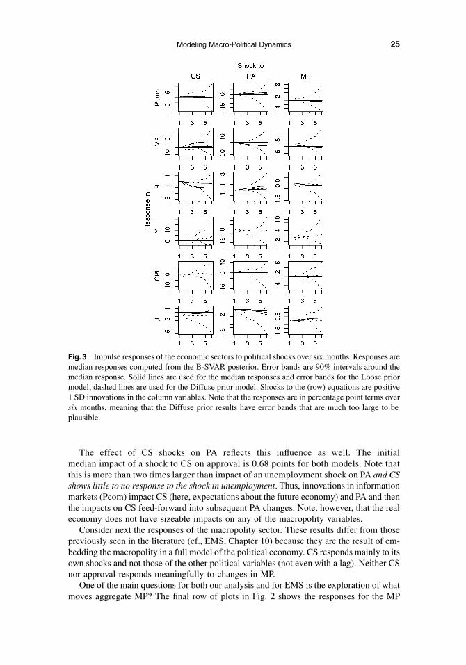
The effect of CS shocks on PA reflects this influence as well. The initialmedian impact of a shock to CS on approval is 0.68 points for both models. Note thatthis is more than two times larger than impact of an unemployment shock on PA and CSshows little to no response to the shock in unemployment. Thus, innovations in informationmarkets (Pcom) impact CS (here, expectations about the future economy) and PA and thenthe impacts on CS feed-forward into subsequent PA changes. Note, however, that the realeconomy does not have sizeable impacts on any of the macropolity variables.

Consider next the responses of the macropolity sector. These results differ from thosepreviously seen in the literature (cf., EMS, Chapter 10) because they are the result of em-bedding the macropolity in a full model of the political economy. CS responds mainly to itsown shocks and not those of the other political variables (not even with a lag). Neither CSnor approval responds meaningfully to changes in MP.

One of the main questions for both our analysis and for EMS is the exploration of whatmoves aggregate MP? The final row of plots in Fig. 2 shows the responses for the MP

Fig. 3 Impulse responses of the economic sectors to political shocks over six months. Responses aremedian responses computed from the B-SVAR posterior. Error bands are 90% intervals around themedian response. Solid lines are used for the median responses and error bands for the Loose priormodel; dashed lines are used for the Diffuse prior model. Shocks to the (row) equations are positive1 SD innovations in the column variables. Note that the responses are in percentage point terms oversix months, meaning that the Diffuse prior results have error bands that are much too large to beplausible.


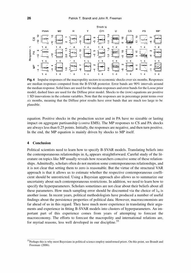
equation. Positive shocks in the production sector and in PA have no sizeable or lastingimpact on aggregate partisanship (contra EMS). The MP responses to CS and PA shocksare always less than 0.25 points. Initially, the responses are negative, and then turn positive.In the end, the MP equation is mainly driven by shocks to MP itself.

4 Conclusion

Political scientists need to learn how to specify B-SVAR models. Translating beliefs intothe contemporaneous relationships in A0 appears straightforward. Careful study of the lit-erature on topics like MP usually reveals how researchers conceive some of these relation-ships. Admittedly, scholars often do not mention some contemporaneous relationships, andit is not clear that setting them to zero is reasonable. But the virtue of the structural VARapproach is that it allows us to estimate whether the respective contemporaneous coeffi-cient should be unrestricted. Using a Bayesian approach also allows us to summarize ouruncertainty about such contemporaneous restrictions. In addition, we need to learn how tospecify the hyperparameters. Scholars sometimes are not clear about their beliefs about allthese parameters. How much sampling error should be discounted via the choice of k0 isanother issue. In recent years, political methodologists have produced a number of usefulfindings about the persistence properties of political data. However, macroeconomists arefar ahead of us in this regard. They have much more experience in translating their argu-ments and experience in fitting B-SVAR models into clusters of hyperparameters. An im-portant part of this experience comes from years of attempting to forecast themacroeconomy. The efforts to forecast the macropolity and international relations are,for myriad reasons, less well developed in our discipline.55

Fig. 4 Impulse responses of the macropolity sectors to economic shocks over six months. Responsesare median responses computed from the B-SVAR posterior. Error bands are 90% intervals aroundthe median response. Solid lines are used for the median responses and error bands for the Loose priormodel; dashed lines are used for the Diffuse prior model. Shocks to the (row) equations are positive1 SD innovations in the column variables. Note that the responses are in percentage point terms oversix months, meaning that the Diffuse prior results have error bands that are much too large to beplausible.

55Perhaps this is why most Bayesians in political science employ uninformed priors. On this point, see Brandt andFreeman (2006).


Important extensions of the B-SVARmodel are being developed. For example, there arenew methods for translating theory into additional restrictions on the effects of laggedendogenous variables (the A1 matrix in the model) and for formally testing these restric-tions (e.g., Cushman and Zha 1997). Some researchers contend that formal models producemore useful structural insights than VAR models (structural, RF and/or Bayesian). Propo-nents of Bayesian time series models reply that formal models often suffer from problemsof observational equivalence and that they are very difficult to fit to data. A more catholicapproach is taken by Sims (2005) who argues that formal models—in the case of macro-economics, Dynamic Stochastic General Equilibrium (DSGE) models—are good for‘‘spinning stories’’ and that these stories ought to be restrained or refined by the resultsof VARs. Work is underway in macroeconomics to try to make this connection more ex-plicit. This work specifically uses DSGE models to develop informed priors for B-SVARmodels. The DSGE models are linearized at the point representing general, macroeco-nomic equilibrium and then the parameter values from the DSGE model are translatedinto the hyperparameters of the B-SVAR model.56

In political science, we lack a well-developed, general equilibrium theory of thekind that spawned DSGE models. However, spatial theory and the new works onelectoral coordination and campaign finance (Mebane 2000; Mebane 2003; Mebane2005) point the way to the development of such theory. The challenge is to join theseworks with the B-SVAR approach to make more sustained progress in the study of themacropolity.57

5 Funding

National Science Foundation (grant numbers SES-0351179 to J.R.F., SES-0351205 andSES-0540816 to P.T.B.).

Appendix: Impulse Responses for Diffuse Prior Model

This appendix contains the impulse responses for the models with the Loose and Diffusepriors. Figures 3 and 4 plot these responses over sixmonths, rather than forty-eightmonthsas in Figs. 1 and 2, to illustrate the explosive nature of the Diffuse prior responses relative tothe Loose prior responses. Using the longer time span would make it impossible to see theLoose prior responses because of the large scale of the Diffuse prior responses. Note thatthe six-month impulse response function results for the Diffuse prior have error bands thatare large and implausible given the historical values of U.S. macroeconomic and politicaldata.

56Ingram and Whiteman (1994) and Del Negro and Schorfheide (2004) draw informed priors from DSGEs forBVARs. Leeper et al. (1996) argue that DSGE models provide insights into the long-term economic dynamicsand VARs into the short-term dynamics of the economy. In a more recent article, Sims (2005) notes that DSGEmodels are better than VARs for ‘‘spinning elaborate stories about how the economy works’’ but expresses someskepticism about whether linearizations of DSGE models usually produce accurate second-order approxima-tions to the likelihood. He goes on to say, ‘‘No one is thinking about the time varying residual variances whenthey specify or calibrate these [DSGE] models.’’ Sims predicts a ‘‘hornet’s nest’’ for macroeconomic DSGEpolicy modelers.

57For a sketch of how this development might occur, see Freeman (2005).


References

Alesina, Alberto, and Howard Rosenthal. 1995. Partisan politics, divided government and the economy. Cam-bridge: Cambridge University Press.

Alesina, Alberto, John Londregan, and Howard Rosenthal. 1993. A model of the political economy of the UnitedStates. American Political Science Review 87:12–33.

Bartels, Larry M. 1991. Instrumental and ‘‘quasi-instrumental’’ variables. American Journal of Political Science35(3):777–800.

Bartlett, M. S. 1957. A comment on D. V. Lindley’s statistical paradox. Biometrika 44(3/4):533–534.Beck, Nathaniel. 1987. Elections and the fed: Is there a political monetary cycle? American Journal of PoliticalScience 31(1):194–216.

Bernanke, B. 1986. Alternative explanations of the money-income correlation. Carnegie-Rochester ConferenceSeries on Public Policy 25(1):49–99.

Bernardo, Jose M. 1979. Reference posterior distributions for Bayesian inference. Journal of the Royal StatisticalSociety. Series B (Methodological) 41(2):113–47.

Bernhard, William, and David Leblang. 2006.Democratic processes and financial markets: Pricing politics. NewYork: Cambridge University Press.

Blanchard, O., and D. Quah. 1989. The dynamic effects of aggregate demand and supply disturbances. AmericanEconomic Review 79:655–73.

Box-Steffensmeier, Janet M., and Renee M. Smith. 1996. The dynamics of aggregate partisanship. AmericanPolitical Science Review 90(3):567–80.

Brandt, Patrick T., and John R. Freeman. 2006. Advances in Bayesian time series modeling and the study ofpolitics: Theory testing, forecasting, and policy analysis. Political Analysis 14(1):1–36.

Brandt, Patrick T., and John T. Williams. 2007. Multiple time series models. Beverly Hills, CA: Sage.Brandt, Patrick T., Michael Colaresi, and John R. Freeman. 2008. The dynamics of reciprocity, accountability, andcredibility. Journal of Conflict Resolution 52:343–74.

Carlin, Bradley P., and Thomas A. Louis. 2000. Bayes and empirical Bayes methods for data analysis. 2nd ed.Boca Raton, FL: Chapman & Hall/CRC.

Chib, Siddartha. 1995. Marginal likelihood from the Gibbs output. Journal of the American Statistical Association90(432):1313–21.

Clarke, Harol D., Karl Ho, and Marianne C. Stewart. 2000. Major’s lesser (not minor) effects: Prime ministerialapproval and governing party support in Britain since 1979. Electoral Studies 19(2–3):255–73.

Clarke, Harol D., and Marianne C. Stewart. 1995. Economic evaluations, prime ministerial approval and govern-ing party support: Rival models reconsidered. British Journal of Political Science 25(2):145–70.

Cortes, Fernando, Adam Przeworski, and John Sprague. 1974. System analysis for social scientists. New York:John Wiley and Sons.

Cushman, David O., and Tao Zha. 1997. Identifying monetary policy in a small open economy under flexibleexchange rates. Journal of Monetary Economics 39:433–48.

De Boef, Suzanna, and James Granato. 1997. Near integrated data and the analysis of political relationships.American Journal of Political Science 41(2):619–40.

De Boef, Suzanna L., and Keele Luke. 2008. Taking time seriously. American Journal of Political Science52:184–200.

Del Negro, Marco, and Frank Schorfheide. 2004. Priors from general equilibrium models for VARs. InternationalEconomic Review 45:643–73.

Doan, Thomas, Robert Litterman, and Christopher Sims. 1984. Forecasting and conditional projection using re-alistic prior distributions. Econometric Reviews 3:1–100.

Edwards, George C., and B. Dan Wood. 1999. Who influences whom? The president and the public agenda.American Political Science Review 93(2):327–44.

Erikson, Robert S., Michael B. MacKuen, and James A. Stimson. 1998. What moves macropartisanship? A re-sponse to Green, Palmquist and Schickler. American Political Science Review 92(4):901–12.

———. 2002. The macropolity. New York: Cambridge University Press.Franzese, Robert F. 2002.Macroeconomic policies of developed democracies, Cambridge studies in comparativepolitics. New York: Cambridge University Press.

Franzese, Robert F., and Jude Hays. 2005. Empirical modeling strategies for spatial interdependence: Omittedvariable vs. simultaneity bias. Paper originally presented at the Annual Meeting of the Political MethodologySociety, Stanford University, Palo Alto, CA.

Freeman, John R. 2005. Modeling macropolitics: EITM and Reality. Paper presented at the EITM Workshop,Canadian Political Science Association Meetings. London: Ontario.


Freeman, John R., John T. Williams, Daniel Houser, and Paul Kellstedt. 1998. Long memoried processes,unit roots and causal inference in political science. American Journal of Political Science 42(4):1289–327.

Freeman, John R., John T. Williams, and Tse-Min Lin. 1989. Vector autoregression and the study of politics.American Journal of Political Science 33:842–77.

Garthwaite, Paul H., Joseph B. Kadane, and Anthony O’Hagan. 2005. Statistical methods for eliciting probabilitydistributions. Journal of the American Statistical Association 100(470):680–700.

Geweke, John. 2005. Contemporary Bayesian econometrics and statistics. Hoboken, NJ: John Wiley & Sons.Gill, Jeff. 2004. Introducing the special issue of political analysis on Bayesian methods. Political Analysis12(4):323–37.

———. 2007.Bayesian methods: A social and behavioral sciences approach. 2nd edn. Boca Raton, FL: Chapmanand Hall.

Goldstein, Joshua, and Jon C. Pevehouse. 1997. Reciprocity, bullying and international cooperation: Time seriesanalysis of the Bosnian conflict. American Political Science Review 91:515–24.

Goldstein, Joshua S., Jon C. Pevehouse, Deborah J. Gerner, and Shibley Telhami. 2001. Reciprocity, triangularity,and cooperation in the Middle East, 1979–1997. Journal of Conflict Resolution 45(5):594–620.

Green, Donald, Bradley Palmquist, and Eric Schickler. 1998. Macropartisanship: A replication and critique.American Political Science Review 92(4):883–900.

Hamilton, James D. 1994. Time series analysis. Princeton, NJ: Princeton University Press.Ingram, Beth F., and Charles H. Whiteman. 1994. Supplanting the ‘Minnesota’ prior: Forecasting macroeconomictime series using real business cycle model priors. Journal of Monetary Economics 34:497–510.

Jackman, Simon. 2004. Bayesian analysis in political science. Annual Reviews of Political Science 7:483–505.

———. 2008. Bayesian analysis for the social sciences. Hoboken, NJ: John Wiley & Sons.Kadane, Joseph B., Ngai Hang Chan, and Lara J. Wolfson. 1996. Priors for unit root models. Journal of Econo-metrics 75:99–111.

Kadiyala, K. Rao, and Sune Karlsson. 1997. Numerical methods for estimation and inference in Bayesian VAR-model. Journal of Applied Econometrics 12:99–132.

Kass, Robert E., and Adrian E. Raftery. 1995. Bayes factors. Journal of the American Statistical Association90(430):773–95.

Leeper, Eric M., Christopher A. Sims, and Tao A. Zha. 1996.What does monetary policy do? Brookings Papers onEconomic Activity 1996(2):1–63.

Litterman, Robert B. 1980. Techniques for forecasting with vector autoregressions. PhD thesis University ofMinnesota.

———. 1986. Forecasting with Bayesian vector autoregressions—Five years of experience. Journal of Business,Economics and Statistics 4:25–38.

Manski, Charles. 1995. Identification problems in the social sciences. Cambridge, MA: Harvard University Press.Martin, Andrew, and Kevin Quinn. 2002. Dynamic ideal point estimation via Markov chain Monte Carlo for theU.S. Supreme Court. Political Analysis 10(2):134–53.

Mebane, Walte R. 2000. Coordination, moderation, and institutional balancing in American Presidential andHouse Elections. American Political Science Review 94:37–53.

———. 2003. Congressional campaign contributions, direct service, and electoral outcomes in the United States:Statistical tests of a formal game model with statistical estimates. Political complexity: Nonlinear models ofpolitics, ed. Diana Richards. Ann Arbor: University of Michigan Press.

———. 2005. Partisan messages, unconditional strategies, and coordination in American Elections. Revisedversion of a paper originally presented at the Annual Meeting of the Political Metholodolgy Society, StanfordUniversity, Palo Alto, CA.

Morris, Irwin L. 2000. Congress, the President, and the Federal Reserve: The politics of American monetarypolicy-making. Ann Arbor: University of Michigan Press.

Ogata, Ktsuhiko. 1967. State space analysis of control systems. Englewood Cliffs, NJ: Prentice-Hall, Inc.Ostrom, Charles, and Renee Smith. 1993. Error correction, attitude persistence, and executive rewards and punish-ments: A behavioral theory of presidential approval. Political Analysis 3:127–84.

Pevehouse, Jon C., and Joshua S. Goldstein. 1999. Serbian compliance or defiance in Kosovo? Statistical analysisand real-time predictions. Journal of Conflict Resolution 43(4):538–46.

Poole, Keith. 1998. Recovering a basic space from a set of issue scales. American Journal of Political Science42:954–93.

Poole, Keith T., and Howard Rosenthal. 1997. Congress: A political-economic history of roll call voting. NewYork: Oxford University Press.


Richard, Jean Francois 1977. Bayesian analysis of the regression model when the disturbances are generatedby an autoregressive process. In New developments in the application of Bayesian methods, eds. A. Aykacand C. Brumat. Amsterdam: North Holland.

Robertson, John C., and EllisW. Tallman. 1999. Vector autoregressions: Forecasting and reality.Economic Review(Atlanta Federal Reserve Bank) 84(1):4–18.

———. 2001. Improving federal funds rate forecasts in VARmodels used for policy analysis. Journal of Businessand Economics Statistics 19(3):324–30.

Sattler, Thomas, John R. Freeman, and Patrick T. Brandt. 2008. Popular sovereignty and the room to maneuver: Asearch for a causal chain. Comparative Political Studies 41(9):1212–39.

———. 2009. Erratum: Popular sovereignty and the room to maneuver: A search for a causal chain. ComparativePolitical Studies 42(1):157–63.

Sims, Christopher A. 1972. Money, income, and causality. American Economic Review 62:540–52.———. 1980. Macroeconomics and reality. Econometrica 48(1):1–48.———. 1986a. Are forecasting models usable for policy analysis? Quarterly Review, Federal Reserve Bank ofMinneapolis 10:2–16.

———. 1986b. Specification, estimation, and analysis of macroeconomic models. Journal of Money, Credit andBanking 18(1):121–6.

———. 2005. The state of macroeconomic policy modeling: Where do we go from here? Macroeconomics andreality, 25 years later. Conference, Barcelona, Spainhttp://www.econ.upf.es/crei/activities/sc_conferences/22/Papers/sims.pdf (accessed April 13, 2005).

Sims, Christopher A., and Tao A. Zha. 1995. Error bands for impulse responses. http://sims.princeton.edu/yftp/ier/(accessed January 15, 2007).

———. 1998. Bayesianmethods for dynamicmultivariate models. International Economic Review 39(4):949–68.———. 1999. Error bands for impulse responses. Econometrica 67(5):1113–56.Theil, Henri. 1963. On the use of incomplete prior information in regression analysis. Journal of the AmericanStatistical Association 58(302):401–14.

Waggoner, Daniel F., and Tao A. Zha. 2003a. A Gibbs sampler for structural vector autoregressions. Journal ofEconomic Dynamics & Control 28:349–66.

———. 2003b. Likelihood preserving normalization in multiple equation models. Journal of Econometrics114:329–47.

Western, Bruce, and Simon Jackman. 1994. Bayesian inference for comparative research. American PoliticalScience Review 88(2):412–23.

Williams, John T. 1990. The political manipulation of macroeconomic policy. American Political Science Review84(3):767–95.

———. 1993a. Dynamic change, specification uncertainty, and Bayesian vector autoregression analysis. PoliticalAnalysis 4:97–125.

———. 1993b. What goes around comes around: Unit root tests and cointegration. Political Analysis 1:229–35.Williams, John T., and Brian K. Collins. 1997. The political economy of corporate taxation. American Journal ofPolitical Science 41(1):208–44.

Wilson, Sven E., and Daniel M. Butler. 2007. A lot more to do: The sensitivity of time-series cross-section anal-yses to simple alternative specifications. Political Analysis 15(2):101–23.

Zellner, A., and A. Siow. 1980. Posterior odds ratios for selected regression hypotheses. In Bayesian statistics:Proceedings of the First International Meeting Held in Valencia, eds. J. M. Bernardo, M. H. DeGroot, D. V.Lindley, and A. F. M. Smith, 585–603. Valencia, Spain: Valencia University Press.

Zha, Tao A. 1998. A dynamic multivariate model for the use of formulating policy. Economic Review (FederalReserve Bank of Atlanta) 83(1):16–29.

———. 1999. Block recursion and structural vector autoregression. Journal of Econometrics 90:291–316.


modeling macro-political dynamicspbrandt/patrick_brandts_website/research_files/... · modeling...

Documents