MODELING NIGHTTIME CHEMISTRY WITH WRF/CHEM:SENSITIVITY TO VERTICAL RESOLUTION AND BOUNDARY LAYER

PARAMETERIZATION

BY

ZANETA KAROLINA GACEK

THESIS

Submitted in partial fulfillment of the requirementsfor the degree of Master of Science in Atmospheric Sciences

in the Graduate College of theUniversity of Illinois at Urbana-Champaign, 2014

Urbana, Illinois

Adviser:

Assistant Professor Nicole Riemer

Abstract

Tropospheric photochemistry and the formation of particulate nitrate depend critically on

the budget of nitrogen oxides (NOx). The NOx budget in turn is tied to the nocturnal

N2O5 hydrolysis reaction, which takes place in the aqueous phase of aerosols. Through this

reaction, NOx is removed from the atmosphere and HNO3 is formed, which then partitions

between the particle and the gas phase. Recent research has shown that these processes

depend crucially on the characteristic development of vertical profiles of gas phase and

aerosol phase species in the nocturnal boundary layer. Resolving these profiles adequately

is a prerequisite for a good representation of nighttime chemistry and poses an important

modeling challenge.

In this work we explore the sensitivity of the model results for N2O5, nitric acid, and

aerosol nitrate to different existing planetary boundary layer parameterizations within the

WRF-Chem model, as well as the sensitivity to model resolution in the vertical direction. We

use a 1-D version of WRF-Chem to systematically investigate a summer and a winter case

of meteorological conditions. In the analysis, we compare the resulting temperature profile

and the vertical profiles of three chemical species, N2O5, HNO3, and aerosol NO3, from five

different planetary boundary layer schemes. Effects of hydrolysis on these chemical species

are also investigated, and we quantify how these results depend on the vertical resolution.

For the summer case, using different boundary layer schemes can change the nocturnal

boundary layer heights by a factor of 2 and the maximum mixing ratios of N2O5 by 22%.

This is in contrast to the winter case, for which the nocturnal planetary boundary depth

varies by a factor of 13 when using different boundary layer schemes, and maximum mixing

ii

ratios of N2O5 vary by 18%. The impact of the hydrolysis reaction is largest for the QNSE

scheme. While changing the vertical resolution has the largest impact on the temperature

profile when using the YSU scheme (a nonlocal scheme), the largest impact on the target

chemical species is seen for the YSU and the QNSE scheme.

iii

To my parents

and Marcelina and Karolina, my sisters

iv

Acknowledgments

Big thanks to my advisor Nicole Riemer, who made this project possible, for all the valuable

comments and insights throughout the entire process of earning my Master’s degree, and

for the smile she always had on her face. I would also like to thank three people from my

research group: Amanda Jones for putting up with my mental breakdowns and for providing

mental comfort during this entire time; Jeffrey Curtis for always willing to help with any

questions or worries I had about WRF/research/classes/job hunting or anything I happened

to mention while at our office - I wouldn’t have survived grad school without the support

of you two; and Wayne Chang for giving me an introduction to modeling with WRF/Chem

and to the chemical processes. Lastly, thank you to my parents, sisters, and Pawe l for all

the love they show me that always gives me the energy to keep going, and to my friends

in the Department of Atmospheric Sciences for making grad school more than just about

research and classes.

v

Table of Contents

Chapter 1 Introduction . . . . . . . . . . . . . . . . . . . . . . . . . . . . . 1

Chapter 2 Background . . . . . . . . . . . . . . . . . . . . . . . . . . . . . . 42.1 Chemistry of Nitric Oxides . . . . . . . . . . . . . . . . . . . . . . . . . . . . 4

2.1.1 Daytime Chemistry . . . . . . . . . . . . . . . . . . . . . . . . . . . . 52.1.2 Nighttime Chemistry . . . . . . . . . . . . . . . . . . . . . . . . . . . 7

2.2 The Planetary Boundary Layer . . . . . . . . . . . . . . . . . . . . . . . . . 92.2.1 The Diurnal Cycle of Planetary Boundary Layer . . . . . . . . . . . . 102.2.2 Turbulence Closure Techniques . . . . . . . . . . . . . . . . . . . . . 11

2.3 Vertical Distribution of Chemical Species . . . . . . . . . . . . . . . . . . . . 13

Chapter 3 Model Description . . . . . . . . . . . . . . . . . . . . . . . . . . 163.1 Boundary Layer Parameterizations . . . . . . . . . . . . . . . . . . . . . . . 17

3.1.1 Local Schemes . . . . . . . . . . . . . . . . . . . . . . . . . . . . . . . 173.1.2 Nonlocal Schemes . . . . . . . . . . . . . . . . . . . . . . . . . . . . . 21

Chapter 4 Setup of Case Studies . . . . . . . . . . . . . . . . . . . . . . . . 234.1 Choice of PBL Schemes . . . . . . . . . . . . . . . . . . . . . . . . . . . . . 234.2 Design of Sensitivity Studies . . . . . . . . . . . . . . . . . . . . . . . . . . . 24

Chapter 5 Results . . . . . . . . . . . . . . . . . . . . . . . . . . . . . . . . . 285.1 Summer Case . . . . . . . . . . . . . . . . . . . . . . . . . . . . . . . . . . . 28

5.1.1 Effects of Boundary Layer Scheme Choice . . . . . . . . . . . . . . . 295.1.2 Effects of Model Vertical Resolution . . . . . . . . . . . . . . . . . . . 38

5.2 Winter Case . . . . . . . . . . . . . . . . . . . . . . . . . . . . . . . . . . . . 445.2.1 Effects of Boundary Layer Scheme Choice . . . . . . . . . . . . . . . 445.2.2 Effects of Model Vertical Resolution . . . . . . . . . . . . . . . . . . . 49

5.3 Effects of Hydrolysis for All Scenarios . . . . . . . . . . . . . . . . . . . . . . 54

Chapter 6 Conclusions . . . . . . . . . . . . . . . . . . . . . . . . . . . . . . 57

References . . . . . . . . . . . . . . . . . . . . . . . . . . . . . . . . . . . . . . 61

vi

Chapter 1

Introduction

Having both natural and anthropogenic sources, nitrogen oxides (NOx) have been of concern

since the earliest studies of air pollution. NOx is a precursor for secondary species such as

ozone and particulate nitrate, each of which contribute to poor air quality. The World

Health Organization (WHO) reported that one in eight deaths globally in 2012 were caused

by air pollution (CNN.com, 2014). Most deaths associated with air pollution are due heart

disease, stroke, chronic obstructive pulmonary disease, and lung cancer, and 80% of them

occur in low and middle-income countries. Policies such as the U.S. Clean Air Act of 1970,

have been developed over time in order to prevent poor air quality days. Even though air

quality has improved in some locations, many regions around the globe still struggle with

this issue. For example, topography in California South Coast Air Basin makes it difficult

for pollutants to be transported over the mountains, persistently leading to the exceeding of

the national ambient air quality standards. Air quality is also a concern in Asia. According

to an April 2014 article from The Wall Street Journal, Beijing, China has only experienced

25 good air quality days between April 2008 and March 2014 using the U.S. standards (The

Wall Street Journal, 2014).

NOx can originate from soils and lightning, but emissions from fossil fuels combustion

processes and biomass burning are its main sources in the atmosphere. During the daytime

the reaction with the OH radical is the major sink for NOx, producing nitric acid (HNO3).

1

The NOx budget is also tied to the nocturnal N2O5 reaction, which takes place in the

aqueous phase of aerosols. Through this reaction, called the heterogeneous hydrolysis, NOx

is removed from the atmosphere and HNO3 is formed, which then partitions between the

particle and the gas phase. The nighttime reaction of N2O5 is therefore important because

it impacts the oxidizing capacity of the atmosphere. It is the focus of this thesis.

The atmospheric chemistry of nitrogen oxides is strongly linked to the dynamics of the

planetary boundary layer. During the day, the sun drives convection and mixing, which leads

to greater boundary layer heights. During the summer, when convection is most prominent,

the height could be even on the order of a few kilometers (Stull, 1988). Pollutants spread

throughout the entire depth of the boundary layer and are usually well mixed. Soon after

the sun sets, the convection shuts down, and the boundary layer becomes much shallower,

sometimes as low as 100 m. Mixing is much less efficient at night, and as a result, pollutants

tend to be more concentrated and vertically stratified (Brown et al., 2007a). Hence, the

depth of the stable boundary layer governs the atmospheric transport and dispersion of

pollutants (Banta et al., 2007).

The heterogeneous hydrolysis reaction of N2O5 is a prime example of the interaction of

transport and chemistry. The efficiency of this reaction depends crucially on the character-

istics of the vertical profiles of gas phase and aerosol species during the nighttime. Resolving

these profiles adequately is a prerequisite for a good representation of nighttime chemistry

and poses an important modeling challenge.

Here we are using the Weather Research and Forecasting model with chemistry (WRF-

Chem, (Grell et al., 2005)) to investigate the sensitivity of the vertical distribution of night-

time chemical species to different existing planetary boundary layer parameterizations and

to the model resolution in the vertical. A summer and a winter case of meteorological condi-

tions are investigated systematically using the single column model (SCM) framework. The

key differences between model configurations with each boundary layer scheme and vertical

resolution are discussed.

2

The next chapter of this thesis, Chapter 2, provides background information on atmo-

spheric chemistry of the species of interest during the day and night, followed by the key

points crucial to understand the basics of boundary layer dynamics. Chapter 2 concludes

with information on the behavior of chemical species within the boundary layer and the

development as well as implications of their vertical profiles. In Chapter 3, the model used

in this study is described, including the different ways of parameterizing boundary layer

physics. Chapter 4 outlines the setup of the model for this research project, and Chapter 5

shows the results from the model runs. This thesis is closed with Chapter 6 with concluding

discussion and avenues for future work.

3

Chapter 2

Background

This chapter provides the foundation to understand vertical profiles of chemical species.

The discussion starts with the basic information about chemistry that governs NOx budget.

Major reactions that cycle over the day and night are shown. Next, the basics of planetary

boundary layer physics as well as its diurnal cycle are reviewed. The two topics are then

combined to explain the various vertical distribution of pollutants throughout the boundary

layer.

2.1 Chemistry of Nitric Oxides

Chemical reactions in the troposphere depend greatly on the budget of nitrogen oxides, or

NOx (Brown et al., 2007b, 2005). NOx is an important primary pollutant that has both

anthropogenic and natural sources. For example, automobiles and fossil fuel combustion

processes release NOx, but it can be also emitted from natural sources such as lightning or

the soil. It then undergoes multiple reactions, discussed below, that lead to the formation

of secondary pollutants, such as ozone and PAN. Reactions during the day differ from those

at night mainly because they are driven by the sun; however, at night the reaction rates

can be increased due to the formation of the nocturnal stable boundary layer that prevents

pollutants from dispersing in the vertical past the top of that layer as discussed further in

section 2.3.

4

2.1.1 Daytime Chemistry

During the day, NO2 is photolyzed by solar radiation for wavelengths λ < 420 nm (Dou-

glas and Huber, 1965) to produce ozone. This process is described by the reactions below

(Atkinson, 2000).

NO2 + hν −−→ NO + O(3P) (R1)

O(3P) + O2 + M −−→ O3 + M (R2)

where M is an inert collision partner, commonly an N2 or O2 molecule. Since O3 quickly

reacts with NO, the following reaction occurs, in which ozone is destroyed:

NO + O3 −−→ O2 + NO2 (R3)

Those three reactions, however, result in no net formation or loss of ozone. For any net

production of ozone, volatile organic compounds, or VOCs, have to be present. VOCs react

with OH and form the intermediate RO2 and HO2 radicals. These two radicals help convert

NO to NO2, which can later be photolyzed to supply the single oxygen molecules O(3P) for

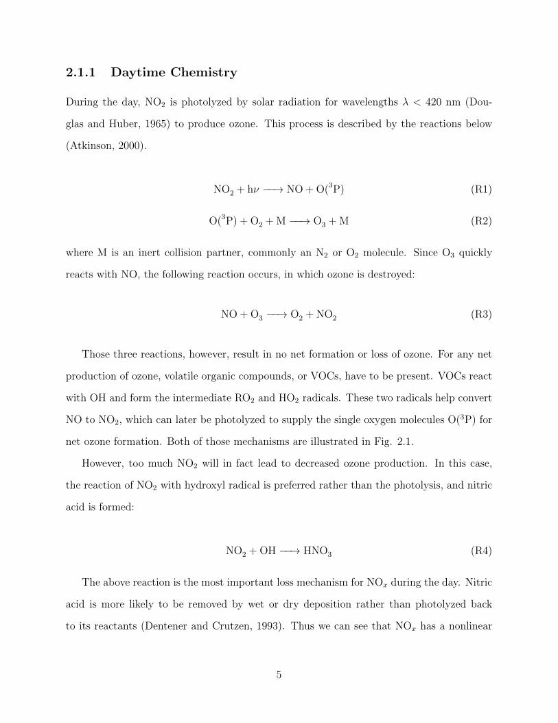
net ozone formation. Both of those mechanisms are illustrated in Fig. 2.1.

However, too much NO2 will in fact lead to decreased ozone production. In this case,

the reaction of NO2 with hydroxyl radical is preferred rather than the photolysis, and nitric

acid is formed:

NO2 + OH −−→ HNO3 (R4)

The above reaction is the most important loss mechanism for NOx during the day. Nitric

acid is more likely to be removed by wet or dry deposition rather than photolyzed back

to its reactants (Dentener and Crutzen, 1993). Thus we can see that NOx has a nonlinear

5

Figure 2.1: Schematics of the reactions involved in NO-to-NO2 conversion and O3 formationin (A) NO-NO2-O3 systems in the absence of VOCs, and (B) NO-NO2-O3 systems in thepresence of VOCs (Atkinson, 2000).

influence on ozone production. Overall, for greatest ozone formation there has to be an

optimum ratio of VOCs to NOx.

Now, the two discussed species, NO2 and O3 can react together and form NO3, which

has been shown to be an important oxidant at night.

NO2 + O3 −−→ NO3 + O2 (R5)

NO3 + hν −−→ NO + O2 (R6)

or

NO3 + hν −−→ NO2 + O (R7)

The reaction of NO3 production (R5) is slower than its destruction, shown in (R6) and

(R7) since the photolysis rate in (R6) and (R7) is large. In addition to photolysis, NO3 can

also react with NO to produce two molecules of NO2. As a result, its daytime concentration

is often negligible because it is easily photolyzed, but increased cloudiness can limit the

6

destruction of NO3 (Brown et al., 2005).

2.1.2 Nighttime Chemistry

After the sun sets, ozone is no longer formed due to the lack of photolysis. Any leftover

ozone can produce NO3, which will not be destroyed by the sunlight. NO3 is the only oxidant

at night and the main driver of chemistry until the sun rises again. It reacts with VOCs,

but one of its most important reactions is the formation of N2O5 (R8) (Morris Jr and Niki,

1973; Geyer et al., 2001).

NO3 + NO2 ←−→ N2O5 (R8)

Concentrations of NO3 and N2O5 depend on shifts in meteorology as well as variations in

NO2 and NO levels (Brown et al., 2003). The ratio of NO3 to N2O5 is temperature dependent

(Dentener and Crutzen, 1993), and the equilibrium for reaction (R8) can be written by

[N2O5]−−Keq[NO2][NO3] (R9)

where K eq is the temperature-dependent equilibrium constant (cm3 molecule−1). N2O5

stability is promoted at lower temperatures. It increases by a factor of 20 when the temper-

ature changes from 0 ◦C to 20 ◦C.

The fate of N2O5 can be determined by two loss pathways: a direct and an indirect

pathway. The direct pathway is the hydrolysis, or the reaction of dinitrogen pentoxide with

water. Dentener and Crutzen (1993) showed that the homogeneous hydrolysis, which means

the reaction with water vapor, is too slow to have any significant impact on N2O5 and NOx

lifetimes. The heterogeneous hydrolysis on and within aerosol particles or cloud droplets,

however, is much faster and acts as a dominant sink for N2O5 in the troposphere.

N2O5(g) + H2O(l) −−→ 2 HNO3(aq) (R10)

7

The rate of change in N2O5 mixing ratio during the heterogeneous hydrolysis is modeled

as a pseudo-first-order process (Heikes and Thompson, 1983; Chang et al., 1987):

d[N2O5]

dt

∣∣∣∣het

= −kN2O5 [N2O5], (2.1)

kN2O5 =1

4cN2O5 · γN2O5 · S (2.2)

where kN2O5 is the rate constant for the heterogeneous surface reaction (Riemer et al., 2003),

cN2O5 is the mean molecular velocity of N2O5, S is the aerosol surface area density and γN2O5

is the reaction probability, or the likelihood of N2O5 uptake on particles. γN2O5 depends on

the aerosol chemical composition, relative humidity, and temperature (Davis et al., 2008).

Higher relative humidity enhanced the hydrolysis, so more nitric acid was produced. This

is because higher relative humidity is linked to greater amount of water in the atmosphere.

The efficiency of hydrolysis also depended on the variations in NO2 concentration, aerosol

composition, and aerosol surface area density. NO2 was one of the reactants required for

N2O5 formation, so N2O5 must be vulnerable to any NO2 gradients. Greater aerosol surface

area density can increase the probability of N2O5 bumping into an aerosol coated with

water and hydrolyze. Also organic coatings on aqueous aerosols can greatly suppress N2O5

heterogeneous hydrolysis; however the relative importance of organic coating is decreased if

the aerosol contains nitrate (Riemer et al., 2009).

Indirect loss pathways include any reactions that could lead to lesser production of the

nitrate radical. If there were no emissions of NO during the night, the reaction below:

NO3 + NO −−→ 2 NO2 (R11)

would be unimportant (Brown et al., 2003). However, in the urban, agricultural, and grass-

land areas sources of NO are very significant. Hence NO could give a rise to vertical gradients

8

in both NO3 and N2O5. The dependence of NO3 and N2O5 levels showed that NO acts as a

dominant sink for these species during night.

NO3 can also be taken up by aerosols or react with dimethyl sulfide (DMS) and hydro-

carbons (Brown et al., 2007b; Allan et al., 2000). Analysis of the measurements showed

that isoprene was a controlling factor for loss of NO3 and N2O5. Isoprene reacts rapidly

with NO3, which will also limit the amount of NOx produced. It can also be oxidized and

removed in locations with very high NOx emissions as they provide large source strength for

NO3. Highest concentration of isoprene at the top of the residual layer was correlated with

negligible concentrations of both NO3 and N2O5. Vertical profiles of NO3 and N2O5 were

anti-correlated with DMS concentration. DMS reacts very rapidly with NO3, preventing

its entrainment out of the nocturnal boundary layer. This explains its steady decrease of

concentration with height, allowing for greater amounts of NO3 and thus N2O5 aloft.

Regardless of the loss pathway, N2O5 fate controls the nighttime lifetime of NOx, and the

heterogeneous hydrolysis of N2O5 is the most important removal process during the night

for NOx. The product of the hydrolysis, nitric acid (HNO3), has a high dry deposition

velocity and is very water soluble, so it is easily removed from the atmosphere by wet or dry

deposition (Hanke et al., 2003).

2.2 The Planetary Boundary Layer

The boundary layer is a thin layer of atmosphere, usually between a few tens of meters to

a few kilometers above the surface of the earth (Stull, 1988; Markowski and Richardson,

2011). In this bottom portion of the troposphere, also referred to as the planetary boundary

layer (PBL), the atmosphere is directly influenced by the presence of the surface fluxes of

heat, moisture, and momentum. Those fluxes are exchanged through mixing within an hour

or less. The flow within the boundary layer is dominated by turbulent eddies resulting from

surface heating and vertical wind shear. The depth is then determined by the intensity of

9

turbulent mixing, which in turn depends on the amount of insolation.

2.2.1 The Diurnal Cycle of Planetary Boundary Layer

During the day, the ground heats up due to the energy input from the sun, promoting

mixing from the surface through conduction at the microscopic scale. The surface is then

much warmer than the atmosphere aloft, leading to an unstable profile. Convection can

occur from thermals rising from the surface that overshoot the top of the boundary layer

and penetrate the stably stratified atmosphere above. This process allows the atmosphere

to mix and the boundary layer to grow. Since mixing causes homogeneity, wind speed

and pollutant concentrations tend to constant with height. One example of a well mixed

pollutant in the daytime boundary layer is ozone. This has implications for the nighttime

distribution of pollutants.

The maximum height of a boundary layer is reached in the late afternoon before sunset,

and with reduced amount of sunlight, mixing diminishes and the boundary layer height

decreases. After the sun sets, heating and turbulent processes due to buoyancy are shut off,

and the only way turbulence can exist is due to shear. Surface cooling due to the infrared

heat loss helps increase stability in the near-ground layer. This is what creates the stable

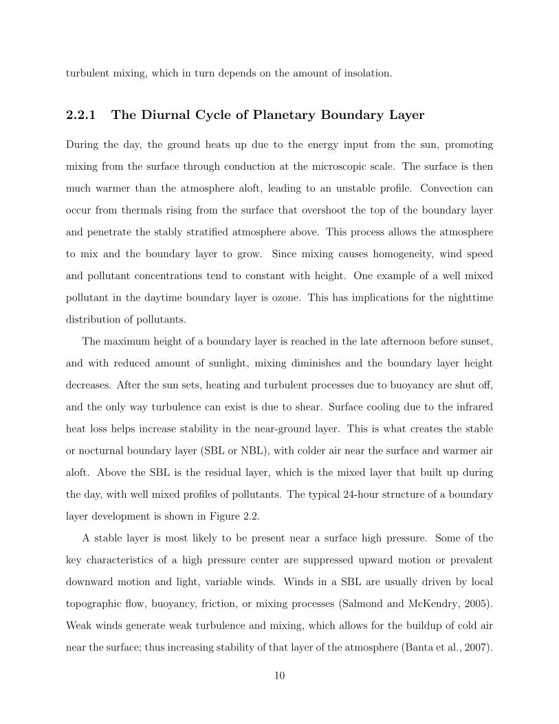
or nocturnal boundary layer (SBL or NBL), with colder air near the surface and warmer air

aloft. Above the SBL is the residual layer, which is the mixed layer that built up during

the day, with well mixed profiles of pollutants. The typical 24-hour structure of a boundary

layer development is shown in Figure 2.2.

A stable layer is most likely to be present near a surface high pressure. Some of the

key characteristics of a high pressure center are suppressed upward motion or prevalent

downward motion and light, variable winds. Winds in a SBL are usually driven by local

topographic flow, buoyancy, friction, or mixing processes (Salmond and McKendry, 2005).

Weak winds generate weak turbulence and mixing, which allows for the buildup of cold air

near the surface; thus increasing stability of that layer of the atmosphere (Banta et al., 2007).

10

2000

1000

0

altit

ude

(m)

noon sunset midnight sunrise noon

local timeA B C D E

capping inversion

free atmosphere

entrainment zone

entrainment zone

mixedlayer

stable boundary layer

residual layer

mixed layer

surface layer surface layer surface layer

Figure 2.2: The structure of a typical boundary layer for a 24-hour period (Markowski andRichardson, 2011).

2.2.2 Turbulence Closure Techniques

Turbulent kinetic energy (TKE) is a measure of the intensity of turbulence, hence it is an

important variable in micrometeorology. The closure problem of the turbulent flow is one of

the unsolved issues of classical physics. It happens when the number of unknown variables

in a set of equations is larger than the number of known equations. That means we do

not have a prognostic or diagnostic equation defining that variable. New equations can be

included for those variables, but they result in even more new unknowns, and this can go

on further without an end.

The order of closures is named by the highest order of the prognostic equations that

are retained, and the next order moments are approximated. However, half order closures

can also be used when given a particular moment category, only a portion of the available

equations are utilized.

Closures can be thought of in two different ways: local and nonlocal. Each has a different

way of treating the exchange between grid boxes as well as the top of the boundary layer and

free atmosphere. For a local closure, the unknown quantity is parameterized by the values

of known quantities at the same point, whereas for a nonlocal closure it is determined from

11

values at many points in space.

Local closures assume turbulence analogous to molecular diffusion. To determine the

eddy diffusivity, K, for local vertical mixing, local schemes use the mixing length scale (L)

and turbulent kinetic energy (TKE) equations. In 1925, Prandtl (1925) defined the mixing

length as the average distance a parcel moves in the mixing process that generated flux.

The TKE equation consists of buoyancy and shear production, dissipation of energy, and

vertical mixing. However, for this theory to be true, the scale of the diffusion mechanism,

or turbulence motion in this case, has to be much smaller than the scale of the mean flow

(Louis, 1979; Pleim and Chang, 1992).

In the case when turbulence scale is greater and more comparable to the mean flow scale, a

nonlocal closure would be more suitable. Nonlocal closure assumes that each eddy transports

fluid like an advection process, so mixing occurs between adjacent and non-adjacent model

layers. This approach is most commonly used in convective boundary layers where mixing is

caused by the buoyant plumes originating in the surface layer (Blackadar, 1978). Nonlocal

schemes diagnose a planetary boundary layer top from the stability profile or Richardson

number and specify a K profile.

The problem of closures can be circumvented by finding parameterizations for the un-

knowns through approximating them in terms of known quantities. A parameter is usually

a constant, the value of which is determined empirically. The greatest differences among the

local schemes lie in the diagnostic length-scale calculations. As for nonlocal schemes, some

include a specified non-local term, Γ, and others add a mass-flux term instead, which is a

flux between non-neighboring layers. Specific parameterizations used in the WRF model

will be discussed in the Chapter 3.

12

2.3 Vertical Distribution of Chemical Species

Some characteristics of the SBL, such as reduced turbulence, which inhibits mixing, and

its shallow depth that affects pollutant concentrations can worsen air quality (Haupt et al.,

2010). Pollutants can accumulate in the SBL, which enhances chemical reactions, possibly

leading to harmful conditions. Primary, or freshly-emitted pollutants have greatest concen-

trations near the surface, which decrease with height due to dilution and reactions with other

chemicals. On the other hand, secondary pollutants, or those produced through chemical

reactions, usually have a maximum higher in the atmosphere. This is due to the loss at the

surface due to dry deposition and little to no production aloft. Depending on the way a

species is produced, the maximum concentration may occur either near the top of the stable

boundary layer or just above it.

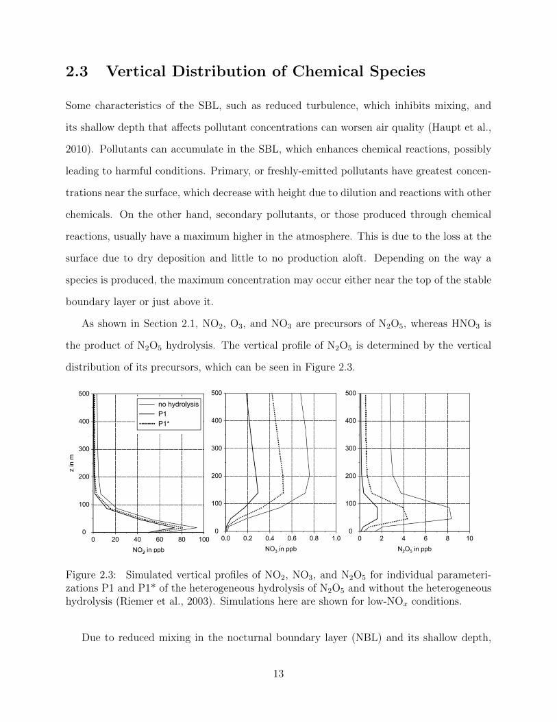
As shown in Section 2.1, NO2, O3, and NO3 are precursors of N2O5, whereas HNO3 is

the product of N2O5 hydrolysis. The vertical profile of N2O5 is determined by the vertical

distribution of its precursors, which can be seen in Figure 2.3.

Figure 2.3: Simulated vertical profiles of NO2, NO3, and N2O5 for individual parameteri-zations P1 and P1* of the heterogeneous hydrolysis of N2O5 and without the heterogeneoushydrolysis (Riemer et al., 2003). Simulations here are shown for low-NOx conditions.

Due to reduced mixing in the nocturnal boundary layer (NBL) and its shallow depth,

13

freshly emitted pollutants tend to accumulate near the surface (Chang et al., 2011). That

can lead to titration of the nitrate radical by NO (R11) or ozone by NO. These reaction

can result in complex vertical concentration gradients in NO3 and N2O5. Vertical profiles of

tropospheric NO3 were first measured and constructed by von Friedeburg et al. (2002) using

the differential optical absorption spectroscopy (DOAS). The study showed the maximum

concentration of NO3 at around 300 m, which is the height where the nocturnal jets are

capable of transporting N2O5 downwind by a distance of 300 km. Since N2O5 depends on

aerosol concentration, its vertical profile becomes even more complicated.

Since NOx is mainly emitted close to the surface, NO2 has its maximum concentration

close to the surface as well. Its concentration decreases with height as the distance from the

source increases. Ozone is depleted within the nocturnal boundary layer by NO and NO2

as it is a highly reactive species. Due to reduced vertical mixing, reactions with NOx and

deposition to surface help create a steep vertical gradient of ozone.

As noted by Riemer et al. (2003), NO3 starts to build up above the nocturnal boundary

layer after sunset, reaching its maximum concentration around midnight. Its production

ceases once all of the NO2 has been consumed by ozone. In the residual layer, concentration

of ozone is constant with height, so the NO3 profile resembles the one of NO2. Later at night

near the surface, the production of NO3 is slowed down due to decreasing ozone concentration

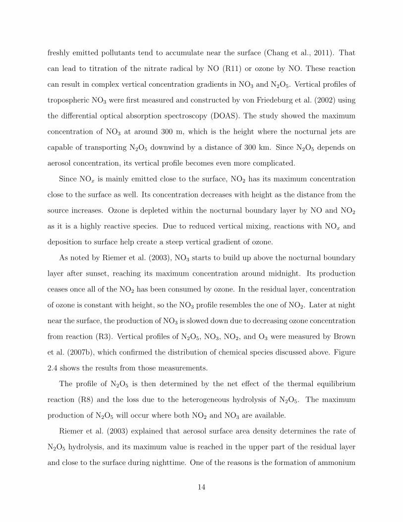
from reaction (R3). Vertical profiles of N2O5, NO3, NO2, and O3 were measured by Brown

et al. (2007b), which confirmed the distribution of chemical species discussed above. Figure

2.4 shows the results from those measurements.

The profile of N2O5 is then determined by the net effect of the thermal equilibrium

reaction (R8) and the loss due to the heterogeneous hydrolysis of N2O5. The maximum

production of N2O5 will occur where both NO2 and NO3 are available.

Riemer et al. (2003) explained that aerosol surface area density determines the rate of

N2O5 hydrolysis, and its maximum value is reached in the upper part of the residual layer

and close to the surface during nighttime. One of the reasons is the formation of ammonium

14

Figure 2.4: Vertical profiles over the Isles of Shoals on 31 July. The open points withinthe mixed boundary layer are from R/V Brown. In the first graph, square indicates NO3,and circle indicates N2O5; and in the second graph, square indicates O3, and circle indicatesNO2 (Brown et al., 2007b).

nitrate, which depends on the availability of ammonia and nitric acid. Ammonium nitrate

as well as N2O5 formation is most favored in low temperatures and high relative humidity

environment. Another explanation is the uptake of water vapor by aerosols. Relative hu-

midity is usually high in those layers, which enhances the increase in aerosol surface area

density. It was noted in Riemer et al. (2003) from vertical profiles that NO3 and HNO3

decrease more slowly with height than N2O5. HNO3 remains in the residual layer from the

day before, and during night, it constantly builds up due to reactions of NO3 with organics

or HO2.

When N2O5 hydrolysis is included in model simulations, concentrations of N2O5, NO3,

and NO2 are reduced, but HNO3, the aerosol surface area density, and the nitrate content of

the aerosol are increased (Riemer et al., 2003). This leads to decreasing ozone in low-NOx

conditions and increasing ozone in high-NOx conditions.

15

Chapter 3

Model Description

The 1-dimensional version of the Weather Research and Forecasting model with chemistry

(WRF-Chem) version 3.3.1 (Grell et al., 2005) was used in this study to simulate the vertical

profiles of meteorological and chemical variables. WRF-Chem is a mesoscale non-hydrostatic

model and has been fully coupled to enable air quality simulations at the same time as the

meteorological model runs, so no temporal interpolations are needed. The model is avail-

able in two different versions of the dynamical core, the Advanced Research WRF (ARW)

used here, and the WRF-NMM (NMM) (University Corporation for Atmospheric Research,

2014). It also features a data assimilation system, and a software architecture allowing for

parallel computation and system extensibility. The development of the model began in late

1990’s by the collaboration of the National Center for Atmospheric Research (NCAR), the

National Oceanic and Atmospheric Administration (represented by the National Centers

for Environmental Prediction (NCEP) and the (then) Forecast Systems Laboratory (FSL)),

the Air Force Weather Agency (AFWA), the Naval Research Laboratory, the University of

Oklahoma, and the Federal Aviation Administration (FAA). The WRF model is used by

more than 20,000 users in over 130 countries.

The idealized single column model (SCM) framework is part of the standard WRF model

distribution. It is configured as a 2x2 mass-grid stencil that is periodic in X and Y directions.

16

All terrain heights are equal (WRF Users Workshop, 2009). The WRF chemistry package

consists of treatments for dry deposition of gases and aerosols, biogenic emission, a complex

photolysis scheme, a state of the art aerosol module, and a choice of chemical mechanism

from RADM2 (Stockwell et al., 1990; Kirchner and Stockwell, 1996), RACM (Stockwell et al.,

1997), CBMZ (Zaveri and Peters, 1999), CB4 (Gery et al., 1989), MOZART (Brasseur et al.,

1998), SAPRC99 (Carter, 2000), or NMHC9 (WRF User’s Guide).

In this chapter we will review the boundary layer parameterizations that are used in

WRF. The discussion begins with the differences between the two major schools of thought,

and then it is divided into sections for local and nonlocal schemes.

3.1 Boundary Layer Parameterizations

Eleven boundary layer parameterization schemes have been implemented into the WRF/Chem

model version 3.3.1. The main differences between them lay in the expression for the eddy

diffusivity (K). The way of parameterizing K varies depending on the order of turbulence

parameterization, and whether it is a local or nonlocal closure. Each scheme also has a

different way of treating entrainment between the top of the boundary layer and free atmo-

sphere.

3.1.1 Local Schemes

In WRF-Chem, the local schemes include Mellor-Yamada-Janjic (MYJ (Janjic, 1994)),

Quasi-Normal Scale Elimination (QNSE (Sukoriansky et al., 2005)), Mellor-Yamada-Nakanishi-

Niino Level 2.5 and 3 (MYNN2 and MYNN3 (Nakanishi and Niino, 2006)), Bougeault-

Lacarrere (BouLac (Bougeault and Lacarrere, 1989)), and University of Washington (UW

(Bretherton and Park, 2009)). Local schemes allow mixing only between the neighbor-

ing grid cells. They are also called the TKE schemes because they use the equation for

turbulent kinetic energy (e) to determine K for local turbulent mixing (WRF tutorial,

17

http://www.mmm.ucar.edu/wrf/users/tutorial/). The TKE equation consists of shear pro-

duction, buoyancy production (or destruction), dissipation of energy, and vertical mixing.

Most of the local schemes are 1.5 order, but they differ most in diagnostic length-scale

computations.

All of the local schemes solve for TKE use

∂(e)

∂t=

1

ρ

∂w′e

∂z− u′w′∂U

∂z− v′w′∂V

∂z+

g

Tvw′T ′v − ε (3.1)

where the first term on the right-hand side represents the vertical divergence of the

vertical transport of TKE by perturbation vertical velocity; the second and third terms are

shear production; the fourth term is buoyancy production, and the fifth term is dissipation.

Horizontal gradients and advection are neglected due to only local transport (LeMone et al.,

2013).

The second moment of a variable S is generally parameterized as:

w′s′ = −KS(∂S

∂z− γS) + E (3.2)

where KS is the eddy diffusivity coefficient, and terms γS and E are added to allow

nonlocal vertical fluxes. They are set to zero for the local schemes. Entrainment is included

in the calculation of KS.

The equation for K takes the following form: K = FLmixe0.5, where Lmix is the master

length scale, and F is the main variable that distinguishes each scheme from one another

(LeMone et al., 2013). BouLac is the simplest out of the local schemes, where F is a constant

equal to 0.4, Lmix is based on how far a parcel can travel vertically with initial velocity equal

to (2e)0.5 as determined from the virtual potential temperature profile. Eddy diffusivity

equation takes the same form for heat and momentum, i.e. KH = KM. For the MY schemes

(MYJ, MYNN2, and MYNN3), F is a function of vertical shear, Lmix, e, and virtual potential

temperature Θv. The parameter Lmix takes a more complicated form than in BouLac.

18

For MYJ KM is a constant fraction of KH (Janjic, 1990),

KH = 1.25KM (3.3)

The solution to the budget equations for TKE in the MY schemes is facilitated by the

introduction of multiple dimensionless variables, parameterizations of which distinguishes

the schemes (Helfand and Labraga, 1988). Calculation of KM and KH is expressed in terms

of the flux Richardson number Rf, length scale l, ∂u/∂z, ∂v/∂z, and stability functions, SM

and SH, respectively (Janjic, 1990). The stability functions are in turn calculated using GM

(dimensionless square of the mean shear), and GH (negative of the dimensionless square of

the Brunt-Vaisala frequency). GM is the same for MYJ and MYNN, and it is given by:

GM =l2

e2

[(∂U

∂z

)2

+

(∂V

∂z

)2]

(3.4)

In MYNN, Nakanishi and Niino (2006) improved the stability function to make it bet-

ter suitable for stable boundary layer. GH is expressed in terms of liquid-water potential

temperature θl and total water content Qw, as shown in equation (3.5):

GH = −(l

e

)2

· gθo·(βθdθldz

+ βqdQw

dz

)(3.5)

where βθ and βq are the turbulent diffusivity coefficients (Mellor and Yamada, 1982;

Nakanishi and Niino, 2004). For MYJ, on the other hand, GH is expressed only in terms of

virtual potential temperature θv (equation 3.6):

GH = −(l

e

)2

· β · g · dθvdz

(3.6)

where β is the coefficient of thermal expansion defined in Mellor and Yamada (1974).

MYNN2.5 is the 1.5 order scheme, for which TKE is prognosed, but all other second order

moments are parameterized, and MYNN3 is the 2nd order scheme. It includes normalized

19

velocity variances and potential temperature variance. The additional complexity of the 2nd

order scheme is denoted by adding a set of empirical constants and resolved second order

variables in the stability function, as show below:

SM = SM2.5 + S ′M (3.7)

SH = SH2.5 + S ′H (3.8)

where S2.5 is the equation given in the 1.5 order scheme, and S ′ is the difference from

the 1.5 order scheme.

The MY schemes have been found to produce insufficient mixing in the SBL (Sukoriansky

et al., 2005). Since stable stratification reduces vertical mixing, this may lead to the develop-

ment of spatial anisotropy (physical properties unequal along different axes) and eventually

shield the overlaying circulation from the surface fluxes. In hopes of solving this problem, a

spectral model called the Quasi-Normal Scale Elimination, or QNSE scheme was developed

specifically for the stable conditions. Non-spectral models (i.e. BouLac, MYJ, and MYNN)

introduce closure assumptions in simple, nearly isotropic flows, which are then extrapolated

into real flows with strong anisotropy and waves (Sukoriansky et al., 2005). Reynolds av-

eraging used in those models to parameterize effects of turbulence does not ’see’ different

processes on different scales and simply lumps all these processes together (Sukoriansky and

Galperin, 2008). QNSE accounts for the combined contribution of turbulence and internal

waves and explicitly resolves the spatial anisotropy (Sukoriansky and Galperin, 2004).

The QNSE model has a different approach of calculating both the master length scale

and the eddy diffusivity:

KM,H = 0.55αM,H(Ri)Lmixe0.5 (3.9)

As seen in the equation above, K is a function of the Richardson number, Ri. Ri is a

20

function of ∆z, ∆u, ∆v, and Θv, where ∆ is the top minus bottom difference taken between

grid points separated by ∆z. For neutral conditions, Ri = 0, αM = 1, and αH = 1.4. For

unstable atmosphere, Ri is negative, and αM,H increases with the absolute value of Ri. For

stable conditions, Ri is calculated based on the spectral method. The vertical eddy viscosity

(νz) and diffusivity (κz) coefficients predicted by the spectral model are used in place of KH

and KM.

Spectral models use the Fourier transform to obtain the state of atmospheric variables.

An important advantage of spectral approach is the possibility of solving pressure exactly

using momentum and continuity equations (Sukoriansky and Galperin, 2008). One of the

variables that needs to be resolved is the modal forcing, f, which is a large-scale external

energy source that may originate from shear instabilities. This variable maintains turbu-

lence in statistically steady state, but it allows the adjustment of energy for every Fourier

mode. The major assumption of this closure is that modal forcing is quasi-Gaussian, which

enables one to derive expressions for the eddy viscosity and eddy diffusivity. Velocity and

temperature responses are obtained from the Green functions, which allows the results to be

in terms of wave numbers, eddy viscosities, eddy diffusivity, and Brunt-Vaisala frequency.

Sukoriansky et al. (2005) claim that the new spectral scheme, unlike the MY schemes,

improves the prediction of turbulence in a stable boundary layer by circumventing certain

shortcomings of the Reynolds stress modeling, which is used to calculate KH and KM in

non-spectral models.

The UW scheme works well with the chemistry part of WRF. However, is was not suitable

for the purpose of this project. The scheme is developed mainly for environments with

shallow convection and moist turbulence, where here we use mostly dry conditions.

3.1.2 Nonlocal Schemes

Nonlocal schemes, such as Yonsei University (YSU (Hong et al., 2006)), Global Forecast

System (GFS (Hong and Pan, 1996)), Asymmetric Convective Model Version 2 (ACM2

21

(Pleim, 2007)), Total Energy-Mass Flux (TEMF (Angevine et al., 2010)), and Medium

Range Forecast (MRF (Hong and Pan, 1996)), allow mixing not only between the neighboring

grid cells, but also any grid cell in the entire domain. Using a transilient matrix, one can

determine what fraction of the specific quantity will go into each grid box within the model

domain (Stull, 1988). The nonlocal schemes diagnose the boundary layer top from potential

temperature profile or Richardson number (WRF tutorial). An eddy diffusivity, or ”K

profile” is specified. For YSU, the eddy diffusivity of momentum, KM is given by:

KM = kwsz(1− z

h)2 (3.10)

for z ≤ h, where h is the convective boundary layer height, k = 0.4 is the von Karman

constant, and ws is the velocity scaling factor. The eddy diffusivity for heat, KH, is then

given by:

KH =KM

Pr(3.11)

where Pr is the Prandtl number. The second moment of variable S is calculated from

equation (3.2) now including the terms that allow for nonlocal mixing. To account for

mixing between non-neighboring grid cells, a non-local term (YSU) or a mass-flux term

(ACM2) is added. YSU treats entrainment at the top of the boundary layer by adding an

asymptotic entrainment flux term at the inversion layer (E in equation (3.2)) proportional

to the surface flux (Hong et al., 2006). Hence, nonlocal schemes, especially YSU, perform

well in a convective environment, where large convective eddies dominate and mix the air

within the layer (LeMone et al., 2013).

22

Chapter 4

Setup of Case Studies

4.1 Choice of PBL Schemes

Based on the discussion in Chapter 3, we chose five schemes to have representatives from each

of the two major schools of thought on parameterizing turbulence. Four local schemes: MYJ,

MYNN2, QNSE, and BouLac along with one nonlocal scheme, YSU, were used in this study.

WRF-Chem was simulated for all the possible PBL scheme choices. A scheme was accepted

for this analysis if it reasonably represented the development of chemical species within

the boundary layer throughout the entire 24 hours of the day. Since nighttime boundary

layer is of concern here, fine vertical resolution is needed to accurately represent the low

magnitude winds that often occur under stable conditions (Seaman et al., 2009). Not all

the schemes are designed to work with such a fine resolution, which ruled out all of the

nonlocal schemes from the analysis, except for YSU. Nonlocal schemes were mainly created

for conditions during which convection dominates, whereas local schemes are more likely to

simulate microscopic motions of pollutants (LeMone et al., 2013). One nonlocal scheme was

important to include since it performs better in the daytime convective boundary layer. The

daytime development of the boundary layer and chemical processes might then affect the

nocturnal profiles of chemical variables.

ACM2 scheme was designed for air quality modeling purposes and is used by the Com-

23

munity Multiscale Air Quality (CMAQ) model (EPA.gov, 2013). However, it has not been

implemented into the chemical part of version 3.3.1. of the WRF/Chem model (Pleim, 2011).

ACM2 does not return the data array with the eddy diffusion coefficient, so WRF/Chem has

to use the minimum default value, which leads to insufficient mixing, especially in the con-

vective boundary layer. Due to the minimal value of eddy diffusion coefficient, the chemical

scalars are not being mixed in the vertical. Hence it could not be used in this study.

4.2 Design of Sensitivity Studies

The emissions inventory was acquired from the EPA 2005 National Emissions Inventory over

the South Coast Air Basin of California. Emissions were averaged over a 50km x 50km grid

centered on Los Angeles, CA at the latitude of +33 ◦ 55’ 33.9594” and longitude of −117 ◦

58’ 25.6794”. The fraction of 0.3 of the original emissions was used since it produced greatest

concentration of ozone, suggesting an atmosphere with high VOC to NOx ratio.

The period of 42 hours was chosen because it is enough time to show the entire nocturnal

cycle accounting for the daytime processes that might affect nighttime results. Since the

formation of N2O5 is favored in cool temperatures, we created idealized scenarios for two

times of year, summer and winter, to see the seasonal variations. For each of the cases, one

date was chosen to represent the warm (June 22nd) and cold (January 22nd) meteorological

conditions. Both summer and winter cases were run for the selected PBL parameterization

schemes listed in Table 4.1. The meteorological data for the simulations was downloaded from

the CISL Research Data Archive website (http://rda.ucar.edu/datasets/ds083.2/). This

data was then interpolated by the WRF Preprocessor System (WPS) to provide the model

with the new forcing file, input sounding, and input soil information.

Since the latitude affects the intensity of the solar radiation, which leads to different

seasonal changes throughout the year, the latitude in the study was chosen to represent the

the Midwest region of the United States. This would serve as the average conditions in most

24

of the United States. The model uses no information on geography, meaning there is no

variation in horizontal grid, so the meteorology would not be affected by orography.

The sensitivity of the model was also tested to its resolution in vertical. Each of the

scheme and each season was run using 30, 60, and 90 layers. For our base case we use 60

vertical layers. To investigate how sensitive the vertical distribution of chemical species and

meteorological variables are to the vertical resolution of the model, each case for the five

choices of PBL scheme was re-run with increased and decreased number of layers. The lower

resolution consisted of 30 vertical layers, and the higher consisted of 90 layers.

Since we are interested in the effect of hydrolysis on the resulting concentrations of chem-

ical species, each set of model configuration was repeated for two chemistry options with

the same chemical mechanisms, but one of them included the N2O5 hydrolysis reactions

and its impacts. The chemistry option used here is the Carbon-Bond Mechanics version Z

(CBMZ) Chemistry with MOSAIC aerosols using Kinetic PreProcessor (KPP) library (op-

tion 170). KPP reads chemical reactions and rate constants from ASCII input file, and then

using the Rosenbrok solver it generates the code for chemistry integration (Damian et al.,

2002). The effects of N2O5 hydrolysis (option 174) were implemented into this chemistry

option by Wayne Chang. This chemistry option incorporates organic coating treatment in

aerosols. The representation of aerosol core that is used for N2O5 heterogeneous hydrolysis

uptake rate calculations is based on Bertram and Thornton (2009) paper. This parameteri-

zation uses aerosol liquid water content and considers nitrate suppression as well as chloride

enhancement in N2O5 uptake rates.

A total of 60 simulations were created. The complete model configuration is presented

in Table 4.1. To quantify the impact of hydrolysis on the model results, the percent change

for each PBL scheme option was calculated using the following formula:

∆C(z, t) =Cno hydr(z, t)− Chydr(z, t)

Chydr(z, t)(4.1)

25

Table 4.1: Table presenting physics options used in WRF for the simulations in the study.

where Cno hydr and Chydr is the concentration or mixing ratio of a chemical species at

the same specified layer and hour of simulation when hydrolysis effects were turned off and

turned on, respectively.

The effects of vertical resolution were calculated similarly:

∆C30 =C30 − C60

C60

(4.2)

∆C90 =C90 − C60

C60

(4.3)

where C30, C60, and C90 are concentrations or mixing ratios of a chemical species for 30,

60, and 90 vertical layers, respectively. The values used in calculations are from the same

hour of model simulation and a layer corresponding to a similar height above the surface

when using various number of vertical layers.

For the summer cases, the nocturnal boundary layer depth corresponds to the height at

which the maximum temperature occurred. This is because for stable boundary layer, the

temperature increases with height, and this is what happens during the night. As soon as

the temperature starts to decrease with height, the layer becomes unstable, which represents

the residual layer.

For the winter cases, the PBL height plotted was obtained from the WRF model results,

using the variable called PBLH. To calculate PBLH, nonlocal schemes find the height at

26

which Ri exceeds a critical value that separates stable from turbulent flow. It usually is

at the maximum entrainment layer. Local schemes find height of capping inversion where

potential temperature lapse rate becomes too positive. It is also the height at which 2∗TKE

drops below a certain value. In stable regime, ratio of variance of vertical velocity deviation

and TKE cannot be smaller than that corresponding to the regime of vanishing turbulence.

In unstable regime, TKE production has to be nonsingular in case of growing turbulence

(Skamarock et al., 2008).

27

Chapter 5

Results

We now present the results from the case studies as outlined in Chapter 4. First we discuss

the summer simulations, starting with PBL scheme sensitivity studies, then we move onto

the sensitivity of the results to the vertical resolution. We then follow the same structure to

discuss winter results. Concentrations of N2O5, HNO3, and NO3 (aerosol) for the simulations

with hydrolysis were compared to the simulations without hydrolysis. HNO3 and NO3

(aerosol) were selected because they are products of the hydrolysis reaction.

Since the winter N2O5 concentrations are very different from the summer concentrations,

the presentation of results is divided into two main sections, one for each season. Each

section is organized into two subsections. First, the effects of boundary layer scheme choice

are analyzed. This subsection also includes the differences in results when hydrolysis effects

are included in model simulations. The second subsection talks about the effects of model

vertical resolution on meteorological and chemical variables.

5.1 Summer Case

First we are discussing the summer case since the results are more straightforward and

uniform among the different model configurations. The thermal equilibrium reaction does

not favor the formation of N2O5 as well due to persistently warmer temperatures.

28

5.1.1 Effects of Boundary Layer Scheme Choice

In this part of the analysis we will focus on the effects of PBL scheme choice for the default

case, in which 60 vertical layers are used. The effects of hydrolysis are also discussed in

this subsection. Time and height above the surface were selected based on the time and

layer during which the maximum N2O5 mixing ratio occurred in the summer cases. No-

hydrolysis summer cases were consistent with their maximums at 35th or 36th hour since

the start of model simulation. Including the effects of hydrolysis in simulations introduced

more variation among the PBL schemes. However, all schemes produced high N2O5 levels

at hour 35 of model simulation. Hour 35 corresponds to 10Z or 5 AM CDT (summer) and

4 AM CST (winter). Most of the maximum N2O5 levels were produced in layers around 80

meters above the surface.

Meteorological variables are not affected by the chemistry option in the model simulation,

hence the differences in temperature profile due to PBL scheme choice are discussed first. As

seen in Figure 5.1, the development of temperature throughout the modeled period in vertical

sense depends on the selection of PBL scheme. One can also note that the temperature at

the surface for each scheme varies, meaning that even over time, the PBL scheme can affect

the development of temperature. In some cases, the difference between temperatures for

YSU and MYNN2.5 at the same vertical layer (163 meters above the surface) is over 3.5

Kelvin. For three (QNSE, MYNN2.5, and BouLac) of the five schemes, this is where the

top of the inversion layer exists (yellow line). The top of the inversion layer is highest for

YSU at 341 meters above the surface. As discussed in Chapter 2, the boundary layer depth

determines the concentration of pollutants, with shallower depths leading to greater values

of pollutant concentrations. It means that differences in the development of temperature

profile among the PBL schemes can affect the evolution of chemical species within the 1-

dimensional column over time.

The horizontal lines Figure 5.1 represent the top of the stable boundary layer determined

29

Figure 5.1: Temperature profile at 5 AM (hour 35) for summer. Colors represent thedifferent PBL parameterization schemes.

by the height at which the top of the inversion layer occurred in the nocturnal profile. The

PBL height varies across the model simulations, as shown in Table 5.1 for 60 layers.

Table 5.1: The depth of the nocturnal boundary layer at 5 AM for summer.

The height in the model (z) is calculated from the base-state geopotential (variable

denoted as ’PHB’) and perturbation geopotential (’PH’) as follows:

z =PHB + PH

g(5.1)

where g is the gravitational acceleration (9.8 m s−2). The heights obtained from this

30

calculation are used in the figures showing vertical profiles of chemical species (Fig. 5.2).

Depending on the PBL scheme, the peak concentration may occur above or within the stable

boundary layer for that same species, so it is necessary to see the behavior of chemistry with

respect to the boundary layer depth (top).

Fig. 5.2 shows the vertical profiles for mixing ratios of N2O5 and HNO3 and concentration

of aerosol NO3. The column on the left shows the results for each PBL scheme with the

hydrolysis effects turned on. The column on the right shows the same, but without the

hydrolysis effects. The colors on the legend describe which PBL scheme each line represents.

For all of the PBL schemes, the peak of N2O5 concentration occurs below the SBL top

for hour 35 analyzed here. The result is the same regardless of the PBL scheme choice as

well as whether hydrolysis is turned on. All PBL schemes produce the the maximum mixing

ratio of N2O5 below the top of the SBL, however, when hydrolysis effects are included, the

maximum values of N2O5 drop by nearly an order of magnitude.

Figures 5.3-5.5 show the differences in concentrations from when the hydrolysis effects are

included (hydrolysis on minus hydrolysis off). The first row shows the mixing ratio difference

for N2O5, the second row for HNO3, and the third row the concentration of aerosol NO3.

The columns represent results for each PBL scheme. The greatest difference is produced by

MYNN2.5 (Fig. 5.4), from 1.8 ppb to 0.3 ppb, and smallest by MYJ (Fig. 5.3), from 1.4

ppb to 0.2 ppb. The differences extend to greater heights above the surface for YSU and

BouLac, especially during the second nighttime period, which suggests these two schemes

allowed formation of N2O5 at higher levels than the other three schemes. The differences

in concentrations can only be observed some time after N2O5 had been produced, hence for

most of the simulation period, especially during the day, the difference is zero.

For all local schemes the maximum is produced one hour earlier when hydrolysis is

included, but for the same time using the nonlocal scheme (YSU). The times ranged from 4

AM to 6 AM, which is soon before the sun rises around 6:10 AM and coolest temperatures

occur. The maximums of N2O5 occur at the same height above the surface for each PBL

31

Figure 5.2: Vertical profiles of N2O5, HNO3, and NO3 at 5 AM for summer. Chemistryoption with hydrolysis is shown on the left and without hydrolysis on the right. Colorsrepresent the different PBL parameterization schemes.

scheme case. The distribution of the product of hydrolysis, HNO3, varies more among the

schemes than it was the case for N2O5. Its concentration depends mainly on the distribution

of N2O5, so the time and height of maximum N2O5 corresponds to very low values of HNO3.

32

Figure 5.3: Contour plots showing the impact of including hydrolysis in model calculationsfor concentration levels of N2O5 (top), HNO3 (middle), and aerosol NO3 (bottom) in summer.Column on the left shows results for YSU and on the right for MYJ. Colors represent thedifference of concentrations with hydrolysis minus without hydrolysis.

When hydrolysis effects are included, the maximum values of HNO3 occurred above the SBL

top for YSU, QNSE, MYNN2.5, and BouLac; and at the SBL top for MYJ. The resulting

vertical profiles changed when hydrolysis was turned off. The maximum occured above the

SBL top for all schemes. However, for some schemes, HNO3 did not have a well defined peak

and was rather more mixed in the vertical. Especially MYNN2.5, but also BouLac have

33

Figure 5.4: Contour plots showing the impact of including hydrolysis in model calculationsfor concentration levels of N2O5 (top), HNO3 (middle), and aerosol NO3 (bottom) in summer.Column on the left shows results for QNSE and on the right for MYNN2.5. Colors representthe difference of concentrations with hydrolysis minus without hydrolysis.

a well-mixed layer of HNO3 extending for over 400 meters. The other two local schemes,

QNSE and MYJ produced a much shallower mixed layer, on the order of 100 to 200 meters,

respectively. The maximum values of concentration are about half of those when hydrolysis

was included, suggesting that the well mixed layer of nitric acid came from its daytime

production in the residual layer.

34

Figure 5.5: Contour plots showing the impact of including hydrolysis in model calculationsfor concentration levels of N2O5 (top), HNO3 (middle), and aerosol NO3 (bottom) in summer.Column shows results for BouLac. Colors represent the difference of concentrations withhydrolysis minus without hydrolysis.

For the hour of analysis, the overall shape of the vertical profile produced by YSU is

almost the same regardless of the effects of hydrolysis. The maximum occurs higher than for

the nonlocal schemes at 538 meters when hydrolysis was included, and at 608 meters when

hydrolysis was turned off with comparable mixing ratios of 2.7 ppb and 2.5 ppb, respectively.

Mixing ratios for the nonlocal schemes show more difference; however, the shape of QNSE

35

vertical profile also does not change much when hydrolysis is turned off. By looking at the

contour plots of difference (Fig. 5.3-5.5), QNSE shows the least HNO3 sensitivity to the

hydrolysis effects overall.

The aerosol phase of NO3 is greatly dependent on the PBL scheme choice. When hydrol-

ysis is included, all schemes produce their maximums within the SBL, but the concentration

varies by about 8 µg/m3 at the peaks. All local schemes show strong stratification of con-

centration near the surface, and BouLac produces the least amount of NO3 at the surface.

BouLac is similar to YSU: The nonlocal scheme mixes nitrate more in addition to the greatest

SBL depth, hence the YSU maximum concentration is lowest of all schemes.

More variation among the PBL schemes is introduced when hydrolysis effects are turned

off, which can be noticed in the right column of Fig. 5.2. For some schemes, the maximum

concentration is reached within the residual layer, about 1.8 km above the surface for YSU

and MYJ, and 2.0 km for BouLac. Within the SBL, all schemes have the greatest concen-

tration at the surface except for QNSE that produces a peak about 50 meters above the

surface.

Overall, MYJ shows the least sensitivity in NO3 concentration to the hydrolysis effects.

All local schemes have the difference stratified the most, especially near the surface within

the SBL. YSU differences extend up to 550 meters above the surface. There is more aerosol

nitrate in the residual layer as well as the SBL when hydrolysis effects are turned on.

Table 5.2 shows the percent change in concentration of all the target species when hy-

drolysis is included. The values represent the result for each PBL scheme.

In summary, N2O5 mixing ratio is the most sensitive out of the analyzed species to the

inclusion of hydrolysis in chemistry parameterization. The results are presented in Table

5.2, which shows the percent change if no hydrolysis was included, considering the reference

case. The differences are presented for N2O5, HNO3, and aerosol NO3 in first, second, and

third row, respectively. In columns shown are results for each PBL scheme. All schemes

showed greater N2O5 mixing ratio when no hydrolysis was included, which confirmed that

36

Table 5.2: Table presenting percent change for N2O5, HNO3, and NO3 when hydrolysiseffects are not included in the model simulation. Values are shown for summer cases withthe default number of vertical layers (60).

each scheme resolved the major mechanism of hydrolysis correctly. The percent change is

greatest when using PBL scheme QNSE. Mixing ratio was greater by 1144.1% for N2O5

when hydrolysis is turned off. The smallest difference for the effects of hydrolysis on N2O5

occurred for YSU at 396.0%.

The other two species are not as sensitive as N2O5, but still a significant number of percent

change was observed when the effects of hydrolysis were included. QNSE produced greatest

difference for HNO3 (−34.3%) and BouLac for NO3 (−75.3%); the smallest differences on

HNO3 were for BouLac (−9.9%) and on NO3 for QNSE (−63.2%).

The only nonlocal scheme used in this analysis, YSU, seems to mix N2O5 and its precur-

sors, including ozone, more than the local schemes. The concentrations are usually spread

more throughout the entire stable boundary layer (below the top specified by the maximum

temperature, thus resulting in lower maximum values for all species besides N2O5 for MYJ

and QNSE.

The concentration gradients are not as pronounced for YSU as they are for all local

schemes, and the SBL depth is greatest at 347.02 meters. QNSE, MYNN2.5, and BouLac

had their SBL top at the same height of 165.65 meters above the surface, where for MYJ it

is at 224.27 meters.

37

5.1.2 Effects of Model Vertical Resolution

In this subsection, the effects of model vertical resolution on cases with hydrolysis effects

turned on will be discussed. Results shown are for model simulations with 30, 60, and 90

vertical layers used. First we will focus on the temperature profile at 5 AM and its differences

due to the vertical resolution.

Figure 5.6 shows the vertical profiles of temperature as simulated by the WRF/Chem

using the default 60 vertical layers with added profiles for decreased (30) and increased (90)

number of vertical layers. All profiles are plotted for the same hour of the simulation.

From the figure one can note that using 30 vertical layers can significantly affect the

vertical profile of temperature. Most of the schemes have about 3 degree Celsius (Kelvin)

difference of temperature at the surface, and there are also some differences from the higher

resolution runs within the stable boundary layer. Three local schemes (MYNN2.5, QNSE,

and MYJ) show almost no difference between the 60 and 90 vertical layer runs. However,

YSU and BouLac show a wide variety in temperature profile development for all three vertical

resolution runs. BouLac shows less difference between 30 and 60 rather than 90 and 60.

As shown earlier in Table 5.1, the vertical resolution also has an impact on the SBL

depth. For the two schemes that have a specific treatment of stable atmospheric conditions,

QNSE and MYNN2.5, the SBL depth is greatest when least number of vertical layers is

used; however, for QNSE the difference is very small, within 5 meters, where for MYNN2.5

the difference is about 183 meters. Differences for the other three schemes fall between 52

and 172 meters.

Next we consider figures showing the vertical profiles of the three target chemical species

(Fig. 5.7). As shown in the figure, N2O5 is the most sensitive species to the vertical

resolution. For YSU, MYJ, and QNSE, N2O5 has a maximum mixing ratio at the very top

of the stable boundary layer when using 30 vertical layers. The lower model resolution is

preventing the results from achieving greater concentration levels as the layer of maximum

38

Figure 5.6: Vertical profiles of temperature for YSU, MYJ, QNSE, MYNN2.5, and BouLacat 5 AM for summer. Colors represent the different number of vertical layers used in themodel simulation.

is not resolved in that simulation. For all other cases, the maximum mixing ratio occurs

around the middle levels of the SBL. All PBL schemes agree on producing lowest values of

N2O5 mixing ratio when only 30 layers are used and higher values the more vertical layers

39

are used in the model. However, QNSE and MYNN2.5 produce slightly lower values with

90 layers as compared to 60 layers.

Figure 5.7: Vertical profiles of N2O5, HNO3, and NO3 at 5 AM for MYNN2.5 (summer).Colors represent the different number of vertical layers.

We will focus on one scheme to discuss the variation in concentrations when using different

vertical resolution. At the end of this subsection, we will compare the results from the one

PBL scheme of choice to the other schemes. MYNN2.5 was chosen for the more thorough

analysis because this scheme has been shown to perform well in high vertical resolution

studies. Its specific treatment of stable conditions lead to the best representation of the PBL

depth and carbon monoxide vertical profile in a study of urban PM10 and PM2.5 pollution

episodes in very stable nocturnal conditions by Saide et al. (2011) as compared to YSU,

MYJ, and QNSE. It has later been used by Saide et al. (2012) to evaluate aerosol indirect

effects in marine stratocumulus clouds and by Zabkar et al. (2013) to simulate a high ozone

40

episode at the surface. All of those studies required high vertical resolution, for which MYNN

was most suitable.

The maximum for N2O5 occurs at 82.3 meters for 30 layers, at 78.0 meters for 60 layers,

and at 53.6 meters for 90 layers. Table 5.3 show values of percent change in concentrations

from the 60-layer runs (increased and decreased vertical resolution). Table is divided into

three parts, each for one species analyzed here. The maximum N2O5 mixing ratio changes

by −49.2% when 30 vertical layers are used and by −23.7% when 90 vertical layers are used,

as compared to 60 vertical layers (mixing ratio of 0.282 ppb).

Table 5.3: Table presenting the difference in mixing ratios or concentration between the30-, 60-, and 90-layer simulations for N2O5, HNO3, and NO3 at layers corresponding to 80meters above the surface. Values shown here are for the summer cases.

Values of differences in concentrations of the three species closest to the surface are shown

in Table 5.4. At the first model layer, the N2O5 values vary between the model resolution

runs. Surface mixing ratio for the run with 60 layers is 0.014 ppb. There is a -0.130 ppb

(98% change) difference in mixing ratio from 60 to 30 layers and 0.014 ppb (927% change)

difference from 60 to 90 layers. For HNO3 the mixing ratios vary from 0.5769 (30 layers) to

0.0151 (90 layers) ppb and for NO3 from 4.1353 (30 layers) to 5.1049 (60 layers) µg/m3.

It is important to note that the height of the first layer of the model depends on the

number of layers used in the simulation. First layer is at 82.3 meters above the surface

41

Table 5.4: Tables presenting the difference in mixing ratios or concentration between the30-, 60-, and 90-layer simulations for N2O5, HNO3, and NO3 at the surface. Values shownhere are for the summer cases.

for 30-layer simulation, 25.7 meters for 60-layer, and 10.5 meters for 90-layer. Between the

vertical resolution runs it can be seen that the concentration of a chemical species can either

increase or decrease closer to the surface. If the model is unable to resolve that, it may have

a significant impact on predicted air quality.

The vertical resolution also has an impact on the stable boundary layer height. The SBL

depth partially governs the concentrations of chemical species. For these same conditions

using MYNN2.5 but varying number of vertical layers, the PBL top occurs from 188.9 meters

with 60 layers to 427.9 meters with 30 layers. These ranges also mostly cover the extremes

among all the schemes.

The peaks in N2O5, HNO3, and NO3 concentrations usually occur within 50 meters for

60- and 90-layer runs. The 30 layer runs result in a greater difference for N2O5 and HNO3:

within 200 meters. For NO3 the peak concentrations are within 50 meters for the 30-layer

run as well, but the maximum occurs in the first layer rather than at an elevated height.

However, this varies among the PBL schemes. The peaks are closer together for QNSE

and MYJ, considering N2O5 and NO3 (nitric acid is the same as for MYNN2.5). The nonlocal

YSU and local BouLac do not show as defined peaks for HNO3 as the other local schemes

42

do. The levels at which the maximum nitric acid occurred are more smoothed out, but more

vertical layers have opposite results for the two schemes in terms of which one produces a

profile with greater overall mixing ratio. YSU shows two peaks with high HNO3 mixing

ratio: one right below and another right above the stable PBL top.

43

5.2 Winter Case

Winter case is more complicated than summer because cooler conditions allow for more

N2O5 formation. In the winter, the nights are longer, so N2O5 has more time to accumulate.

Greater mixing ratios lead to more variability among schemes, thus choosing one particular

time at which N2O5 maximum occurred for all schemes was not feasible. The maximum

N2O5 mixing ratio also varies in the vertical, hence for simplicity we are choosing the same

time and height above surface as we did for summer.

The differences in N2O5 mixing ratios are about 2.3 times greater and extend up to much

greater heights above the surface. In the summer, the differences would only be observed

within 600 meters, and in the winter they go up to nearly 2.2 km (BouLac and MYNN2.5).

5.2.1 Effects of Boundary Layer Scheme Choice

As in section 5.1.1, we will again focus on the model results with 60 vertical layers. The

differences due to hydrolysis will be compared among each of the five PBL schemes. We

first consider Fig. 5.8, in which the temperature profile is shown in different colors for each

scheme.

The temperature profile does not vary much across the PBL schemes, especially from

the surface until about 800 meters. The MYNN2.5 scheme produces a constant tempera-

ture profile for about 100 meters above the surface, whereas the other four schemes have a

constantly decreasing temperature until tropopause.

The top of the SBL varies greatly across the schemes, which is shown in Fig. 5.5. The

smallest depth is produced by MYNN2.5 at 65.1 meters and greatest by YSU 376.1 meters

and QNSE 342.5 meters. The low SBL depth can be seen on the vertical temperature

profile. The layer with the constant temperature is the residual layer from the day before,

so anything below that layer will - in case of nighttime - be the stable layer.

We next consider the vertical profiles of the chemical species for all PBL schemes. Fig. 5.9

44

Figure 5.8: Temperature profile at 4 AM (hour 35) for winter. Colors represent the differentPBL parameterization schemes.

Table 5.5: The depth of the nocturnal boundary layer at 4 AM for winter.

shows those vertical profiles for each scheme in a different color, similarly to the temperature

profiles. On the left are the resulting concentrations when hydrolysis is turned on, and on

the right are the results with hydrolysis turned off.

The peak N2O5 mixing ratios at 4 AM occurred higher above the surface when hydrolysis

was not included. For all of the schemes with no hydrolysis, except for QNSE, that peak

was produced above the SBL top. When hydrolysis is included, more schemes report their

maximums below the SLB top (YSU, QNSE, and BouLac). However, in the overall model

simulation, the maximum with no hydrolysis is shown at 8 AM of the second night (hour 39)

for all the schemes, but with hydrolysis it occurs between hour 9 and 15 of the simulation

45

Figure 5.9: Vertical profiles of N2O5, HNO3, and NO3 at 5 AM for winter. Chemistry optionwith hydrolysis is shown on the left and without hydrolysis on the right. Colors representthe different PBL parameterization schemes.

(10Z through 16Z or 4 AM through 10 AM the first night).

Nitric acid has much greater mixing ratios for all PBL schemes within the SBL when

hydrolysis is included (up to 0.04 ppb for MYNN2.5). With no hydrolysis, the values fall

46

down to less than 0.005 ppb (MYNN2.5). There are also no distinct peaks within the SBL.

For NO3 no hydrolysis cases, all schemes are in agreement to within 1 µg/m3 until the

profile reaches 1.4 km. The maximum concentrations are at the surface, and then the NO3

values keep decreasing. The profiles for both hydrolysis cases are divided into MYNN2.5-

BouLac and YSU-MYJ-QNSE groups, where their profiles agree very closely with the other

scheme(s) in the group. However, including hydrolysis introduces more variation, and at

the peak concentration the concentrations differ by about 5 µg/m3. For the three schemes

(YSU, QNSE, and BouLac), the concentrations reach their maximum within the SBL, where

for the other two they are above the SBL.

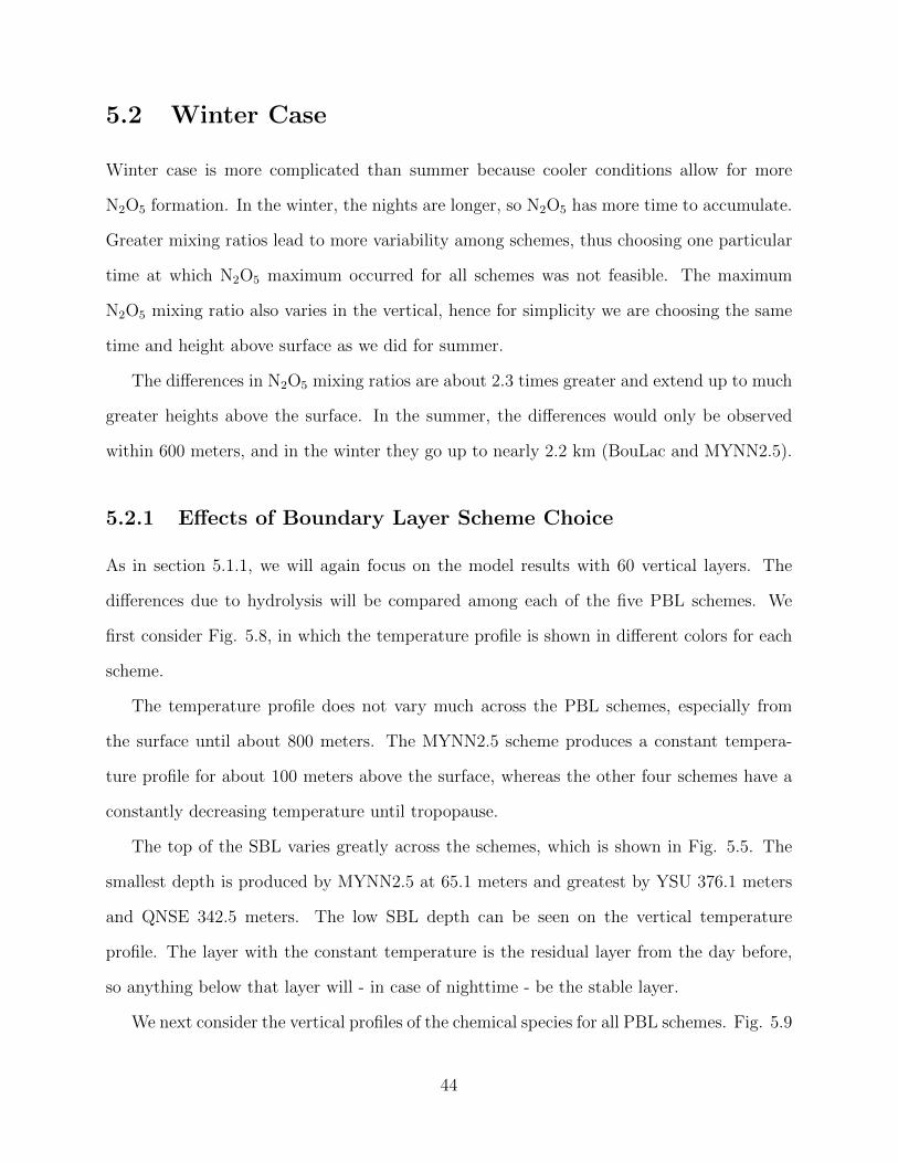
Figures 5.10-5.12 show the differences in mixing ratios and concentration when the hy-

drolysis effects are turned on. Like for summer analysis, the rows show N2O5, HNO3, and

aerosol NO3, respectively from top to bottom, and columns show the results for the PBL

scheme.

Hydrolysis has a large effect on the resulting N2O5 and NO3. The greatest overall dif-

ference occurs shortly before sunrise for all PBL schemes. The lowest difference in N2O5

mixing ratio occurs when MYNN2.5 is used; however, the difference for this scheme spreads

through the higher model levels as compared to the other schemes. Overall, hydrolysis has

similar effects on N2O5 among the PBL schemes.

The concentrations of NO−3 vary slightly more than those for N2O5. Using YSU results

in the greatest difference for the longest period of time, soon before and after the sunrise.

The difference is about 18 µg/m3. However, BouLac and MYNN2.5 show the differences up

to 2.2 km, and MYNN2.5 is the least sensitive to the hydrolysis effects throughout the entire

period and all vertical layers.

The nitric acid shows the least difference possibly due to its partitioning into the aerosol

phase. Where the other two species show the greatest differences, HNO3 has almost no

difference. During night and soon before sunrise, MYJ and QNSE show nearly no difference

at the surface whether hydrolysis is included. The other three schemes show the most

47

Figure 5.10: Contour plots showing the impact of including hydrolysis in model calculationsfor concentration levels of N2O5 (top), HNO3 (middle), and aerosol NO3 (bottom) in winter.Column on the left shows results for YSU and on the right for MYJ. Colors represent thedifference of concentrations with hydrolysis minus without hydrolysis.

difference soon after the sunset, at the beginning of major N2O5 formation.

From Table 5.6 one can note for the time of analysis (4 AM), between 772.7 (BouLac)

and 1640.1 (QNSE) % change for N2O5 occurs when hydrolysis is turned off. On the other

hand, hydrolysis produces from 61.1 (QNSE) to 91.0 (MYNN2.5) % more of HNO3 and

from 74.1 (BouLac) to 77.5 (YSU) % more of aerosol NO3. Similarly to summer cases, the

48

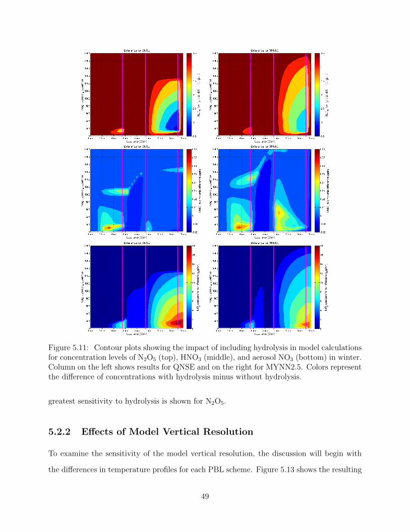
Figure 5.11: Contour plots showing the impact of including hydrolysis in model calculationsfor concentration levels of N2O5 (top), HNO3 (middle), and aerosol NO3 (bottom) in winter.Column on the left shows results for QNSE and on the right for MYNN2.5. Colors representthe difference of concentrations with hydrolysis minus without hydrolysis.

greatest sensitivity to hydrolysis is shown for N2O5.

5.2.2 Effects of Model Vertical Resolution

To examine the sensitivity of the model vertical resolution, the discussion will begin with

the differences in temperature profiles for each PBL scheme. Figure 5.13 shows the resulting

49

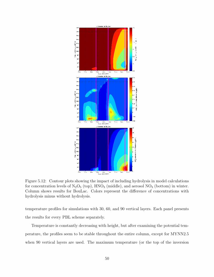
Figure 5.12: Contour plots showing the impact of including hydrolysis in model calculationsfor concentration levels of N2O5 (top), HNO3 (middle), and aerosol NO3 (bottom) in winter.Column shows results for BouLac. Colors represent the difference of concentrations withhydrolysis minus without hydrolysis.

temperature profiles for simulations with 30, 60, and 90 vertical layers. Each panel presents

the results for every PBL scheme separately.

Temperature is constantly decreasing with height, but after examining the potential tem-

perature, the profiles seem to be stable throughout the entire column, except for MYNN2.5

when 90 vertical layers are used. The maximum temperature (or the top of the inversion

50

Table 5.6: Table presenting percent change for N2O5, HNO3, and NO3 when hydrolysiseffects are not included in the model simulation. Values are shown for winter cases with thedefault number of vertical layers (60).

layer) occurs at 94.3 meters above the surface. Overall, all the schemes are not very sensi-

tive to the vertical resolution when considering only temperature (contrary to the summer

case). MYJ and QNSE show the least difference throughout the entire vertical depth shown.

Within the SBL, the most difference is produced by BouLac and YSU, but the differences

are less than 1 Kelvin.

We will again focus on the MYNN2.5 scheme for a more thorough analysis, as chosen

for the summer cases. We will then shortly compare MYNN2.5 to the other schemes. For

this (and MYJ) scheme, the SBL depth calculated by the model was the lowest out of all

schemes. MYNN2.5 produced a very similar depth with 60 and 90 layers at 39.4 and 37.8

meters, respectively. The 30-layer run, however, produced a 331.9-meter deep layer at 4 AM.

The implications of this result can be seen on the vertical profiles of N2O5 HNO3, and

NO3. These profiles are shown in Fig. 5.14.

The chemical species are responding to the depth of the SBL, and the 30-layer run

produced the least maximum concentrations at that time. The pollutants are more diluted

for this case. In the higher resolution runs, more abrupt peaks are observed, especially for

N2O5 mixing ratio. However, for the 30-layer run, the maximum concentrations occur within

the calculated SBL, and for the higher-resolution runs, they occur just above the SBL top.

Comparing the 4 AM N2O5 at the height chosen for summer cases (about 80 meters

above the surface), the mixing ratio is 19.4% less when using 30 layers and only 8.6% less

when using 90 layers. The NO3 concentration varies even less for the vertical resolution

51

Figure 5.13: Vertical profiles of temperature for YSU, MYJ, QNSE, MYNN2.5, and BouLacat 5 AM for winter. Colors represent the different number of vertical layers used in the modelsimulation.

sensitivity runs (2.0% and 5.1% greater with 30 and 90 layers, respectively). However, there

is a large variation among the different vertical resolutions for HNO3. This is true for the

other PBL schemes. The mixing ratio only changes by 1.8% for 30 layers but 25.1% for 90

52

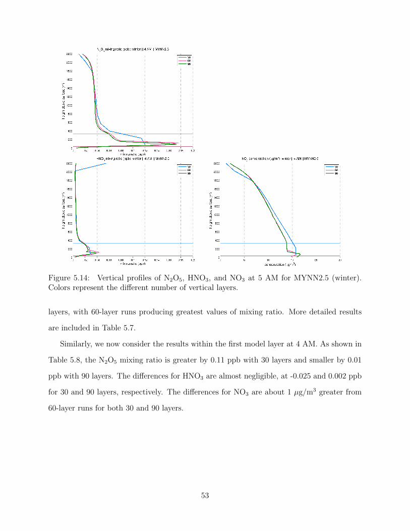
Figure 5.14: Vertical profiles of N2O5, HNO3, and NO3 at 5 AM for MYNN2.5 (winter).Colors represent the different number of vertical layers.

layers, with 60-layer runs producing greatest values of mixing ratio. More detailed results

are included in Table 5.7.

Similarly, we now consider the results within the first model layer at 4 AM. As shown in

Table 5.8, the N2O5 mixing ratio is greater by 0.11 ppb with 30 layers and smaller by 0.01

ppb with 90 layers. The differences for HNO3 are almost negligible, at -0.025 and 0.002 ppb

for 30 and 90 layers, respectively. The differences for NO3 are about 1 µg/m3 greater from

60-layer runs for both 30 and 90 layers.

53

Table 5.7: Table presenting the difference in mixing ratios or concentration between the30-, 60-, and 90-layer simulations for N2O5, HNO3, and NO3 at layers corresponding to 80meters above the surface. Values shown here are for the winter cases.

Table 5.8: Tables presenting the difference in mixing ratios or concentration between the30-, 60-, and 90-layer simulations for N2O5, HNO3, and NO3 at the surface. Values shownhere are for winter cases.

5.3 Effects of Hydrolysis for All Scenarios

Both the PBL scheme and the vertical resolution choice can affect how the modeled concen-

trations of N2O5, HNO3, and NO−3 respond to the addition of the heterogeneous hydrolysis

of N2O5. From Table 5.9 and 5.10 one can note that out of the three analyzed species, N2O5

is the most sensitive to the hydrolysis effects, especially in the winter.

The greatest differences in N2O5 mixing ratios occurred mostly when the QNSE scheme

54

Table 5.9: Tables presenting percent change for N2O5, HNO3, and NO3 when hydrolysiseffects are not included in the model simulation. Values are shown for summer cases witheach vertical resolution.

Table 5.10: Tables presenting percent change for N2O5, HNO3, and NO3 when hydrolysiseffects are not included in the model simulation. Values are shown for winter cases witheach vertical resolution.

was used. While the low-resolution runs, being the least sensitive to hydrolysis, result in

percent changes as low as 149.4% in the summer, in the winter they may be up to 5 times

55

greater. The highest resolution was the most sensitive to hydrolysis, with values up to

1319.2% in the summer and 1742.5% in the winter.

Nitric acid varies between −9.9% and −53.8% in the summer, and between −23.6% and

−92.2% in the winter. For aerosol nitrate those numbers vary from −57.2% and 77.9% in

the summer, and −73.2% and −77.7% in the winter.

56

Chapter 6

Conclusions

The focus of this thesis was to determine the sensitivity of the WRF/Chem model results

for nighttime chemistry to the vertical resolution and the choice of planetary boundary

layer parameterization schemes. We investigated this question by running the WRF/Chem

model for a summer and a winter set of meteorological conditions, each with increased and

decreased vertical resolution, and repeated this process for five PBL schemes. We focused on

concentrations of three nighttime chemical species, N2O5, HNO3, and aerosol NO3, for each

of the aforementioned scenarios and also quantified the impact of including the heterogeneous

hydrolysis of N2O5.

Regardless of the PBL scheme, chemistry option, season, or vertical resolution, the gen-

eral shape of the vertical profiles of N2O5, HNO3, and NO3 were qualitatively resolved in

agreement with observations previously discussed in literature. Mixing ratios of N2O5 re-

sulted in peak levels either within or slightly above the top of the SBL, with lower values

at the surface. When no hydrolysis effects were considered, more N2O5 was produced in the

winter than in the summer. This is consistent with the thermal equilibrium reaction and

longer nights during which N2O5 can form. As expected, very little HNO3 existed during the

night since there was no production due to the OH radical after the sunset. In the summer,

more HNO3 was formed during the day and stayed in the atmosphere through the night

due to the longer time during which OH could exist. The concentration of aerosol NO3 are

57

consistent with both summer and winter temperature profiles. Minimum nighttime aerosol

nitrate concentrations occurred near the top of the inversion layer for summer profiles. In the

winter profile, where temperature was decreasing through the entire troposphere, maximum

concentration occurred near the surface.

For both seasons, the greatest negative difference in N2O5 mixing ratio for all PBL

schemes occurred soon before sunrise. This difference means that if no hydrolysis is included

in the model, N2O5 would be allowed to accumulate until the sun rises. However, hydrolysis,

which acts as a sink for N2O5 removed it from the atmosphere before more could accumulate.

This difference also corresponds to the greatest positive difference in nitric acid in summer.

Formation of nitric acid was enhanced when hydrolysis effects were included since it was the

product of this reaction. Any N2O5 leftover past the sunrise would dissociate back to NO3

and NO2, hence the greatest difference in aerosol NO3 happened after the sun rises, and it

was dependent on the resulting N2O5 mixing ratio before sunrise. Winter HNO3 was less

sensitive to hydrolysis effects and more variable among the schemes. Very little HNO3 exists

in the gas phase during cold conditions because everything partitions into the aerosol phase.

For the summer case, using different boundary layer schemes can change the nocturnal

boundary layer heights by a factor of 2. Temperature profiles have similar shapes for the

local schemes, and the nonlocal scheme is warmer at the surface but cooler aloft until the top

of the nocturnal boundary layer. The differences in temperatures range up to 3.5 Kelvin.

The maximum mixing ratios of N2O5 varied by 22%, by 15% for HNO3, and by 33% for

aerosol NO3 when using different PBL schemes.

For the winter case, the nocturnal planetary boundary depth varies by a factor of 13 when

using different boundary layer schemes. In contrast to the summer case, the temperature

profiles were almost identical among the PBL schemes. The maximum mixing ratios of N2O5

varied by 18%, by 4% for HNO3, and by 17% for aerosol NO3, which was less than in the

summer cases.

Including hydrolysis introduced more variability among the PBL schemes; however, all

58

schemes produced results consistent with observations. Results for winter N2O5 mixing ratio

were greater than for summer if each scheme was considered individually. However, some

schemes in the winter produced so little N2O5 that it was less than the summer mixing ratio

for other schemes. Peak N2O5 mixing ratios occurred in the same layer (within the SBL)

in the summer, regardless of hydrolysis effects. In the winter, those peaks occurred higher

(above the SBL top) when hydrolysis was not included.

At the hour chosen for the analysis in this thesis, both summer and winter HNO3 mixing

ratios resulted in greater values when hydrolysis was turned on, but in the summer this

difference was very small for YSU, and in the winter for MYJ and QNSE. For aerosol NO3,

including hydrolysis resulted in a significant increase of concentrations for both seasons. The

peaks were, however, more extreme in summer cases.

YSU and BouLac often presented similar results, for example temperature and nitric

acid vertical profile for the vertical resolution sensitivity runs in summer. Compared to

the other schemes, YSU produced qualitatively different profiles for all three target species.

As the only nonlocal scheme considered in this analysis, it is likely due to the effects of

mixing between the non-neighboring model grid points. Concentration gradients were not

as pronounced and often produced the lowest maximum values of concentration. The depth

of the stable boundary layer was also greatest for this scheme during winter and summer

simulations.

Considering both seasons and all PBL schemes, there seems to be less differences between

the 60 and 90 vertical layers runs than 60 and 30 vertical layers. The temperature profile was

not very sensitive to vertical resolution in the winter. However, in the summer simulations,

there was up to 3 Kelvin difference between the 30, 60, or 90 vertical-layer runs. Concerning

the chemical species, increasing the number of vertical layers in most simulations did not

end up in more extreme values of the peak concentrations.

For the same hour of simulation (hour 35 analyzed here), the 90-layer runs did not produce

more extreme vertical profiles than the 60-layer runs. In the most extreme case, the largest

59

difference occurred for summer profiles of HNO3 and NO3 when YSU was used, but the

vertical gradients were not as pronounced than for the other PBL schemes. For other cases

that difference was really small (the lines on the graph were almost overlapping). Winter

profiles resulted in less extreme differences, but 90-layer runs produced larger gradients for

most cases than the 60-layer runs.

Aerosol nitrate is an important contributor of PM2.5. Depending on the choice of the

PBL scheme, the surface aerosol nitrate concentration may vary by about 17%. Increasing

or decreasing the vertical resolution of the model may affect the concentrations by about

34%, especially in the summer. Both of the components of this analysis are important in

predicting the air quality.

The analysis performed in this thesis could be repeated for a wider range of meteorological

conditions with various temperature and relative humidity profiles. This would confirm

whether the differences we saw for the two days we chose were representative of the season.

Moreover, the scope of this work was to perform an intercomparison of different PBL schemes

and to quantify the differences. It would be interesting to identify which scheme performs

best in the stable nighttime conditions. This would require the comparison of the model

results to field observations.

60

References

Allan, B. J., McFiggans, G., Plane, J., Coe, H., and McFadyen, G. G. (2000). The nitrateradical in the remote marine boundary layer. Journal of Geophysical Research: Atmo-spheres (1984–2012), 105(D19):24191–24204.

Angevine, W. M., Jiang, H., and Mauritsen, T. (2010). Performance of an eddy diffusivity–mass flux scheme for shallow cumulus boundary layers. Monthly Weather Review, 138(7).

Atkinson, R. (2000). Atmospheric chemistry of vocs and nox. Atmospheric environment,34(12):2063–2101.

Banta, R. M., Mahrt, L., Vickers, D., Sun, J., Balsley, B. B., Pichugina, Y. L., and Williams,E. J. (2007). The very stable boundary layer on nights with weak low-level jets. Journalof the Atmospheric Sciences, 64(9).

Bertram, T. and Thornton, J. (2009). Toward a general parameterization of N2O5 reactivityon aqueous particles: the competing effects of particle liquid water, nitrate and chloride.Atmospheric Chemistry and Physics, 9(21):8351–8363.

Blackadar, A. (1978). Modeling pollutant transfer during daytime convection. In Symposiumon Turbulence, Diffusion, and Air Pollution, 4 th, Reno, Nev, pages 443–447.

Bougeault, P. and Lacarrere, P. (1989). Parameterization of orography-induced turbulencein a mesobeta–scale model. Monthly Weather Review, 117(8):1872–1890.

Brasseur, G., Hauglustaine, D., Walters, S., Rasch, P., Muller, J.-F., Granier, C., andTie, X. (1998). Mozart, a global chemical transport model for ozone and related chemicaltracers: 1. model description. Journal of Geophysical Research: Atmospheres (1984–2012),103(D21):28265–28289.

Bretherton, C. S. and Park, S. (2009). A new moist turbulence parameterization in thecommunity atmosphere model. Journal of Climate, 22(12).

Brown, S., Dube, W., Osthoff, H., Wolfe, D., Angevine, W., and Ravishankara, A. (2007a).High resolution vertical distributions of no3 and N2O5 through the nocturnal boundarylayer. Atmos. Chem. Phys, 7(1):139–149.

Brown, S., Stark, H., Ryerson, T., Williams, E., Nicks Jr, D., Trainer, M., Fehsenfeld, F., andRavishankara, A. (2003). Nitrogen oxides in the nocturnal boundary layer: Simultaneous

61

in situ measurements of NO3, N2O5, NO2, NO, and O3. Journal of Geophysical Research,108(D9):4299.

Brown, S. S., Dube, W. P., Osthoff, H. D., Stutz, J., Ryerson, T. B., Wollny, A. G.,Brock, C. A., Warneke, C., de Gouw, J. A., Atlas, E., et al. (2007b). Vertical profilesin no3 and N2O5 measured from an aircraft: Results from the noaa p-3 and surface plat-forms during the new england air quality study 2004. Journal of Geophysical Research,112(D22):D22304.

Brown, S. S., Osthoff, H. D., Stark, H., Dube, W. P., Ryerson, T. B., Warneke, C., de Gouw,J. A., Wollny, A. G., Parrish, D. D., Fehsenfeld, F. C., et al. (2005). Aircraft observationsof daytime no3 and N2O5 and their implications for tropospheric chemistry. Journal ofPhotochemistry and Photobiology A: Chemistry, 176(1):270–278.

Carter, W. P. (2000). Implementation of the saprc-99 chemical mechanism into the models-3framework. Report to the United States Environmental Protection Agency, January, 29.

Chang, J., Brost, R., Isaksen, I., Madronich, S., Middleton, P., Stockwell, W., and Walcek,C. (1987). A three-dimensional eulerian acid deposition model: Physical concepts andformulation. Journal of Geophysical Research, 92(D12):14681–14.

Chang, W. L., Bhave, P. V., Brown, S. S., Riemer, N., Stutz, J., and Dabdub, D. (2011).Heterogeneous atmospheric chemistry, ambient measurements, and model calculations ofN2O5: A review. Aerosol Science and Technology, 45(6):665–695.

CNN.com (2014). 7 million premature deaths annually linked to air pollution.http://www.who.int/mediacentre/news/releases/2014/air- pollution/en/. ac-cessed in April, 2014.

Damian, V., Sandu, A., Damian, M., Potra, F., and Carmichael, G. R. (2002). The ki-netic preprocessor kpp-a software environment for solving chemical kinetics. Computers& Chemical Engineering, 26(11):1567–1579.

Davis, J., Bhave, P., and Foley, K. (2008). Parameterization of N2O5 reaction probabilities onthe surface of particles containing ammonium, sulfate, and nitrate. Atmospheric Chemistryand Physics, 8(17):5295–5311.

Dentener, F. J. and Crutzen, P. J. (1993). Reaction of N2O5 on tropospheric aerosols:Impact on the global distributions of NOx, o3, and oh. Journal of Geophysical Research,98(D4):7149–7163.

Douglas, A. and Huber, K. (1965). The absorption spectrum of no2 in the 3 700-4 600 aregion. Canadian Journal of Physics, 43(1):74–81.

EPA.gov (2013). Planetary boundary layer modeling for meteorology and air quality.http://www.epa.gov/amad/Research/Air/pbl.html. accessed in January, 2014.

62

Gery, M. W., Whitten, G. Z., Killus, J. P., and Dodge, M. C. (1989). A photochemical ki-netics mechanism for urban and regional scale computer modeling. Journal of GeophysicalResearch: Atmospheres (1984–2012), 94(D10):12925–12956.

Geyer, A., Alicke, B., Konrad, S., Schmitz, T., Stutz, J., and Platt, U. (2001). Chemistryand oxidation capacity of the nitrate radical in the continental boundary layer near berlin.Journal of Geophysical Research: Atmospheres (1984–2012), 106(D8):8013–8025.

Grell, G. A., Peckham, S. E., Schmitz, R., McKeen, S. A., Frost, G., Skamarock, W. C.,and Eder, B. (2005). Fully coupled online chemistry within the wrf model. AtmosphericEnvironment, 39(37):6957–6975.

Hanke, M., Umann, B., Uecker, J., Arnold, F., and Bunz, H. (2003). Atmospheric mea-surements of gas-phase hno3 and so2 using chemical ionization mass spectrometry duringthe minatroc field campaign 2000 on monte cimone. Atmospheric Chemistry and Physics,3(2):417–436.

Haupt, S. E., Wyngaard, J., Young, G., and Long, K. (2010). Modeling the stable boundarylayer depth and quantifying its uncertainty for dispersion. Technical report, AmericanMeteorological Society.

Heikes, B. G. and Thompson, A. M. (1983). Effects of heterogeneous processes on no3,hono, and hno3 chemistry in the troposphere. Journal of Geophysical Research: Oceans(1978–2012), 88(C15):10883–10895.

Helfand, H. and Labraga, J. (1988). Design of a nonsingular level 2.5 second-order closuremodel for the prediction of atmospheric turbulence. Journal of the atmospheric sciences,45(2):113–132.

Hong, S.-Y., Noh, Y., and Dudhia, J. (2006). A new vertical diffusion package with anexplicit treatment of entrainment processes. Monthly Weather Review, 134(9):2318–2341.

Hong, S.-Y. and Pan, H.-L. (1996). Nonlocal boundary layer vertical diffusion in a medium-range forecast model. Monthly weather review, 124(10):2322–2339.

Janjic, Z. I. (1990). The step-mountain coordinate: Physical package. Monthly WeatherReview, 118(7):1429–1443.

Janjic, Z. I. (1994). The step-mountain eta coordinate model: Further developments of theconvection, viscous sublayer, and turbulence closure schemes. Monthly Weather Review,122(5):927–945.

Kirchner, F. and Stockwell, W. R. (1996). Effect of peroxy radical reactions on the predictedconcentrations of ozone, nitrogenous compounds, and radicals. Journal of GeophysicalResearch: Atmospheres (1984–2012), 101(D15):21007–21022.

LeMone, M. A., Tewari, M., Chen, F., and Dudhia, J. (2013). Objectively determined fair-weather cbl depths in the arw-wrf model and their comparison to cases-97 observations.Monthly Weather Review, 141(1):30–54.

63

Louis, J.-F. (1979). A parametric model of vertical eddy fluxes in the atmosphere. Boundary-Layer Meteorology, 17(2):187–202.

Markowski, P. and Richardson, Y. (2011). Mesoscale meteorology in midlatitudes, volume 2.John Wiley & Sons.

Mellor, G. L. and Yamada, T. (1974). A hierarchy of turbulence closure models for planetaryboundary layers. Journal of the Atmospheric Sciences, 31(7):1791–1806.

Mellor, G. L. and Yamada, T. (1982). Development of a turbulence closure model forgeophysical fluid problems. Reviews of Geophysics, 20(4):851–875.

Morris Jr, E. and Niki, H. (1973). Reaction of dinitrogen pentoxide with water. The Journalof Physical Chemistry, 77(16):1929–1932.

Nakanishi, M. and Niino, H. (2004). An improved mellor–yamada level-3 model with con-densation physics: Its design and verification. Boundary-layer meteorology, 112(1):1–31.

Nakanishi, M. and Niino, H. (2006). An improved mellor–yamada level-3 model: its numer-ical stability and application to a regional prediction of advection fog. Boundary-layermeteorology, 119(2):397–407.

Pleim, J. E. (2007). A combined local and nonlocal closure model for the atmosphericboundary layer. part i: Model description and testing. Journal of Applied Meteorology &Climatology, 46(9).

Pleim, J. E. (2011). Comment on simulation of surface ozone pollution in the central gulfcoast region using wrf/chem model: sensitivity to pbl and land surface physics. Advancesin Meteorology, 2011.

Pleim, J. E. and Chang, J. S. (1992). A non-local closure model for vertical mixing in theconvective boundary layer. Atmospheric Environment. Part A. General Topics, 26(6):965–981.

Prandtl, L. (1925). Uber die ausgebildete turbulentz. Zamm, 155.

Riemer, N., Vogel, H., Vogel, B., Anttila, T., Kiendler-Scharr, A., and Mentel, T. (2009).Relative importance of organic coatings for the heterogeneous hydrolysis of N2O5 duringsummer in europe. Journal of Geophysical Research: Atmospheres (1984–2012), 114(D17).

Riemer, N., Vogel, H., Vogel, B., Schell, B., Ackermann, I., Kessler, C., and Hass, H.(2003). Impact of the heterogeneous hydrolysis of n2o5 on chemistry and nitrate aerosolformation in the lower troposphere under photosmog conditions. Journal of geophysicalresearch, 108(D4):4144.

Saide, P., Spak, S., Carmichael, G., Mena-Carrasco, M., Yang, Q., Howell, S., Leon, D.,Snider, J. R., Bandy, A. R., Collett, J. L., et al. (2012). Evaluating wrf-chem aerosolindirect effects in southeast pacific marine stratocumulus during vocals-rex. AtmosphericChemistry & Physics, 12(6).

64

Saide, P. E., Carmichael, G. R., Spak, S. N., Gallardo, L., Osses, A. E., Mena-Carrasco,M. A., and Pagowski, M. (2011). Forecasting urban pm10 and pm2.5 pollution episodesin very stable nocturnal conditions and complex terrain using wrf–chem co tracer model.Atmospheric Environment, 45(16):2769–2780.

Salmond, J. and McKendry, I. (2005). A review of turbulence in the very stable noctur-nal boundary layer and its implications for air quality. Progress in Physical Geography,29(2):171–188.

Seaman, N., Gaudet, B., Zielonka, J., and Stauffer, D. (2009). Sensitivity of vertical struc-ture in the stable boundary layer to variations of the wrf models mellor–yamada–janjicturbulence scheme.. Boulder, 23e27 June, page 7.

Seinfeld, J. H. and Pandis, S. N. (2012). Atmospheric chemistry and physics: from airpollution to climate change. John Wiley & Sons.

Skamarock, W., Klemp, J., Dudhia, J., Gill, D., Barker, D., Duda, M., Huang, X., Wang,W., and Powers, J. (2008). A description of the advanced research wrf version 3. NCARtechnical note NCAR/TN/u2013475.

Stockwell, W. R., Kirchner, F., Kuhn, M., and Seefeld, S. (1997). A new mechanism forregional atmospheric chemistry modeling. Journal of Geophysical Research: Atmospheres(1984–2012), 102(D22):25847–25879.

Stockwell, W. R., Middleton, P., Chang, J. S., and Tang, X. (1990). The second generationregional acid deposition model chemical mechanism for regional air quality modeling.Journal of Geophysical Research: Atmospheres (1984–2012), 95(D10):16343–16367.

Stull, R. B. (1988). An introduction to boundary layer meteorology, volume 13. Springer.

Sukoriansky, S. and Galperin, B. (2004). A spectral-closure model for turbulent flows withstable stratification. Marine Turbulence: Theories, Observations and Models, edited by H.Baumert, J. Simpson, and J. Sundermann, pages 53–65.

Sukoriansky, S. and Galperin, B. (2008). Anisotropic turbulence and internal waves in stablystratified flows (qnse theory). Physica Scripta, 2008(T132):014036.

Sukoriansky, S., Galperin, B., and Perov, V. (2005). Application of a new spectral theory ofstably stratified turbulence to the atmospheric boundary layer over sea ice. Boundary-layermeteorology, 117(2):231–257.

The Wall Street Journal (2014). Beijing’s bad air days, finally counted. http://

blogs.wsj.com/chinarealtime/2014/04/14/beijings-bad-air-days-finally

-counted/. accessed in April, 2014.

University Corporation for Atmospheric Research (2014). The weather research and fore-casting model. http://wrf-model.org/index.php. accessed in February, 2014.

65

von Friedeburg, C., Wagner, T., Geyer, A., Kaiser, N., Vogel, B., Vogel, H., and Platt, U.(2002). Derivation of tropospheric no3 profiles using off-axis differential optical absorptionspectroscopy measurements during sunrise and comparison with simulations. Journal ofGeophysical Research: Atmospheres (1984–2012), 107(D13):ACH–5.

WRF Users Workshop (2009). A description of the wrfv3.1 single columnmodel. http://www.mmm.ucar.edu/wrf/users/workshops/WS2009/ presentations/

5B-03.pdf. accessed in December, 2013.

Zabkar, R., Koracin, D., and Rakovec, J. (2013). A wrf/chem sensitivity study using en-semble modelling for a high ozone episode in slovenia and the northern adriatic area.Atmospheric Environment, 77:990–1004.

Zaveri, R. A. and Peters, L. K. (1999). A new lumped structure photochemical mechanismfor large-scale applications. Journal of Geophysical Research: Atmospheres (1984–2012),104(D23):30387–30415.

66