modeling of an electroactive polymer hydrogel for optical ... · the hydrogel by solving...

i

Modeling of an Electroactive Polymer

Hydrogel for Optical Applications

Robert Alan Paxton

A thesis submitted to the Auckland University of Technology

in fulfilment of the degree of

Doctor of Philosophy in Mechanical Engineering

Auckland, New Zealand

© 2006 by Robert A Paxton

ii

I hereby declare that I am the sole author of this thesis.

I authorise the Auckland University of Technology to lend this thesis to other

institutions or individuals for the sole purpose of scholarly research.

____________________

Robert A. Paxton

I futher authorise the Auckland University of Technology to reproduce this thesis by

photocopying or by other means, in total or in part, at the request of other instituitions

or individuals for the sole purpose of scholarly research.

____________________

Robert A. Paxton

iii

Borrowers Page

The Auckland University of Technology requires the signatures of all persons using or

photocopying this thesis. Accordingly, all borrowers are required to fill out this page.

Date Name Address Signature

iv

Acknowledgements

A project of this size does not reach completion without the assistance and support of

many different people. Firstly, I wish to acknowledge the guidance and support of my

primary supervior, Dr Ahmed Al-Jumaily. His infinite wisdom and encouragement were

invaluable in this work, and allowed it to grow and develop until it reached the form

shown here today. Although contact with my second supervisor, Prof Allan Easteal, was

not as frequent as I would have liked, it was always comforting to know that I had an

expert in polymer chemistry close at hand. I am sure his contributions will continue to

be invaluable to this research. I must also thank my third supervisor, Dr Max Ramos,

who was always ready to help with the nuances of finite element modeling, and who

could help to provide a solid explanation when things didn’t go exactly to plan.

To my colleagues and friends at the DCRC who made me smile, and put up with my

ranting and raving about computers that didn’t do what they were told! In particular to

Gijs, who always managed to distract me with a game of Revolt when the stress became

just a little too much. To Alex, Ibtisam, Ingrid, Joe, Prasika and Yasser and who all

helped in their own small way to keep me sane and to make sure this project reached

completion. There are also numerous other staff, without whom this project could not

have been completed. Chris, Yan and Anita in the 6th floor chemistry labs, who put up

with my many strange requests, and made sure that I had the right equipment with

which to do experiments. Also to Ross, Mark and Bradley in the workshop, who did

their best to make any equipment that I couldn’t purchase directly.

Lastly, to my family: Alan, Patsy, Laurie, Dave, Chris and Pam whose unfailing support

and belief in both me and this work has been invaluable in the last three years. Finally,

and most importantly, to my life’s partner and best friend, Maree, who read this

manuscript almost as many times as me, and without whom this project would never

have reached completion.

To all of these people, I offer my heartfelt thanks and gratitude. This work stands as a

testament of your love and support.

v

Abstract

In this work a finite element model is proposed to describe the swelling of poly(acrylic

acid) hydrogels under the influence of an external electric field. The specific application

of this model is for optical applications, but the design could be used equally well for

other applications such as sensors and actuators.

The model is proposed as five individual modules, which work in conjunction with each

other but which can also function independently. This independence allows the model to

provide intermediate results to the user, and also permits each module to be improved or

adjusted individually without affecting the operation of the overall model. The first

module is the Electrical module, which calculates the external electric field present in

the hydrogel by solving Laplace’s equation. The second module is the Chemical

module, which uses the electric field to calculate the diffusion and migration of ions

through the hydrogel/solvent regions. The third module is the Force module, which uses

the change in ion concentrations to calculate the resulting change in osmotic pressure

(force). This force is then used in the Mechanical module to calculate the deformation

of the hydrogel, based on the assumption of linear elasticity. Finally, the fifth module is

the Optical module, which uses the deformation to calculate the theoretical change in

focal length.

To verify the operation of the model, numerous experiments were conducted with the

deformation of a poly(acrylic acid) hydrogel being measured under various external

voltages with different electrode configurations. Overall, the model agrees quite well

with the experimental results, but also highlights some interesting discrepancies that

will need to be considered in future work. There is also some scope for improvement in

the experimental method used, but again this is left for future work.

vi

Table of Contents

BORROWERS PAGE .................................................................................................................................. III ACKNOWLEDGEMENTS............................................................................................................................IV ABSTRACT................................................................................................................................................V TABLE OF CONTENTS ..............................................................................................................................VI TABLE OF FIGURES..................................................................................................................................IX

1. INTRODUCTION ............................................................................................................................ 1

1.1. BACKGROUND............................................................................................................................ 1 1.2. REVIEW OF LITERATURE............................................................................................................ 7

1.2.1. Models Describing Hydrogel Swelling ................................................................................... 10 1.2.2. The Use of Polymer Hydrogels as Optical Elements .............................................................. 14 1.2.3. Development of a Model to Describe Hydrogel Swelling....................................................... 15

2. OVERALL MODEL ...................................................................................................................... 21

2.1. INTRODUCTION ........................................................................................................................ 21 2.2. THEORETICAL DEVELOPMENT ................................................................................................. 23 2.3. IMPLEMENTATION IN CODE...................................................................................................... 26

2.3.1. Predefined Parameters ........................................................................................................... 26 2.3.2. Time-Integration Loop............................................................................................................ 29

3. ELECTRICAL MODULE............................................................................................................. 31

3.1. INTRODUCTION ........................................................................................................................ 31 3.2. ASSUMPTIONS.......................................................................................................................... 31

3.2.1. Geometrical Assumptions ....................................................................................................... 31 3.2.2. Material Property Assumptions .............................................................................................. 32

3.3. THEORETICAL DEVELOPMENT ................................................................................................. 33 3.3.1. Initial Voltage Distribution..................................................................................................... 33 3.3.2. Boundary Conditions .............................................................................................................. 36

3.4. IMPLEMENTATION IN CODE...................................................................................................... 37

4. CHEMICAL MODULE................................................................................................................. 48

4.1. INTRODUCTION ........................................................................................................................ 48 4.2. ASSUMPTIONS.......................................................................................................................... 49 4.3. THEORETICAL DEVELOPMENT ................................................................................................. 50

4.3.1. Initial Ion Concentrations....................................................................................................... 50 4.3.2. Determination of the Mass Transport Equations.................................................................... 53

4.4. IMPLEMENTATION IN CODE...................................................................................................... 67 4.4.1. Initial Ion Distributions – Solvent Region .............................................................................. 67 4.4.2. Initial Ion Distributions – Hydrogel Region........................................................................... 69 4.4.3. Mass Transport Equations...................................................................................................... 73

vii

5. FORCE MODULE ......................................................................................................................... 79

5.1. INTRODUCTION ........................................................................................................................ 79 5.2. THEORETICAL DEVELOPMENT ................................................................................................. 80

5.2.1. Osmotic Pressure Due to Ionic Interactions........................................................................... 80 5.2.2. Osmotic Pressure Due to Mixing............................................................................................ 83 5.2.3. Translation of Force Vector ................................................................................................... 85

5.3. IMPLEMENTATION IN CODE...................................................................................................... 87 5.4. TRANSLATION OF FORCE VECTOR ........................................................................................... 92

6. MECHANICAL MODULE ........................................................................................................... 93

6.1. INTRODUCTION ........................................................................................................................ 93 6.2. ASSUMPTIONS.......................................................................................................................... 93 6.3. THEORETICAL DEVELOPMENT ................................................................................................. 94

6.3.1. Element Stiffness Matrix [K] .................................................................................................. 95 6.3.2. Element Mass Matrix [M]..................................................................................................... 100 6.3.3. Element Damping Matrix [C]............................................................................................... 102 6.3.4. Boundary Conditions ............................................................................................................ 103 6.3.5. Velocity and Displacement Through Time Integration......................................................... 104

6.4. IMPLEMENTATION IN CODE.................................................................................................... 106

7. OPTICAL MODULE ................................................................................................................... 111

7.1. INTRODUCTION ...................................................................................................................... 111 7.2. ASSUMPTIONS........................................................................................................................ 111 7.3. THEORETICAL DEVELOPMENT ............................................................................................... 112

7.3.1. Analysis of Data from the Mechanical Module .................................................................... 112 7.3.2. Curve Fitting to a Parabola.................................................................................................. 113 7.3.3. Curve Fitting to a Circle....................................................................................................... 114 7.3.4. Relating the Curvature to the Refractive Power................................................................... 115

7.4. IMPLEMENTATION IN CODE.................................................................................................... 115

8. EXPERIMENTAL VALIDATION............................................................................................. 118

8.1. INTRODUCTION ...................................................................................................................... 118 8.2. PREPARATION OF HYDROGELS............................................................................................... 118 8.3. HYDROGEL SWELLING DYNAMICS......................................................................................... 122 8.4. MECHANICAL AND OPTICAL PROPERTIES .............................................................................. 126 8.5. FORCE GENERATED BY POLYMER HYDROGEL ....................................................................... 128

9. RESULTS AND DISCUSSION ................................................................................................... 129

9.1. INTRODUCTION ...................................................................................................................... 129 9.2. ELECTRICAL MODULE ........................................................................................................... 129 9.3. CHEMICAL MODULE .............................................................................................................. 137 9.4. FORCE MODULE..................................................................................................................... 146 9.5. MECHANICAL MODULE.......................................................................................................... 149

viii

9.6. OPTICAL MODULE ................................................................................................................. 159 9.7. OVERALL MODEL .................................................................................................................. 165

10. CONCLUSION ........................................................................................................................ 166

11. REFERENCES......................................................................................................................... 170

APPENDIX A: RAW EXPERIMENTAL DATA................................................................................ 182

A.1 RESULTS FROM ELECTRICAL MODULE................................................................................... 182 A.2 RESULTS FROM FORCE MODULE............................................................................................ 183 A.3 RESULTS FROM MECHANICAL MODULE................................................................................. 183 A.4 RESULTS FROM OPTICAL MODULE......................................................................................... 185 A.5 RAW VIDEO FRAMES ............................................................................................................. 187

APPENDIX B: LISTING OF MATLAB CODE ................................................................................. 192

FLOWCHART OF OVERALL MODEL....................................................................................................... 195 CHEMMOD.M CODE LISTING ................................................................................................................. 196 CONTROL.M CODE LISTING................................................................................................................... 200 DRAW.M CODE LISTING ........................................................................................................................ 204 EFIELD1.M CODE LISTING ..................................................................................................................... 206 EFIELD2.M CODE LISTING ..................................................................................................................... 210 EFIELD3.M CODE LISTING ..................................................................................................................... 214 FEASMBL1.M CODE LISTING ................................................................................................................. 217 FEELDOF.M CODE LISTING .................................................................................................................... 217 FEKINE2D.M CODE LISTING .................................................................................................................. 218 FELP2DT3.M CODE LISTING .................................................................................................................. 218 FELP2DT3B.M CODE LISTING ................................................................................................................ 219 FELPT2T3.M CODE LISTING................................................................................................................... 219 FEMATISO.M CODE LISTING .................................................................................................................. 220 FLAGER.M CODE LISTING...................................................................................................................... 221 FORCE_CHANGER.M CODE LISTING ...................................................................................................... 222 FORCER.M CODE LISTING...................................................................................................................... 222 GEL_DISTRIBUTE.M CODE LISTING ....................................................................................................... 226 GLOBECORD.M CODE LISTING .............................................................................................................. 228 GLOBECORD2.M CODE LISTING ............................................................................................................ 228 MECH.M CODE LISTING ........................................................................................................................ 229 MMTRIANG.M CODE LISTING ................................................................................................................ 230 NODALCON.M CODE LISTING ................................................................................................................ 231 NODALCON2.M CODE LISTING .............................................................................................................. 232 OPTICAL.M CODE LISTING .................................................................................................................... 233

ix

Table of Figures

Figure 2-1: Overall model...............................................................................................22

Figure 2-2: Area coordinates of an element....................................................................24

Figure 2-3: Nodes associated with solvent and hydrogel................................................28

Figure 2-4: Predefined parameters section of overall model ..........................................29

Figure 3-1: Electrical module..........................................................................................31

Figure 3-2: Model geometry ...........................................................................................32

Figure 3-3: System of connected nodes ..........................................................................35

Figure 3-4: Boundary and "air" nodes ............................................................................37

Figure 3-5: Different hydrogel/solvent geometries.........................................................38

Figure 3-6: Symmetry around y-axis ..............................................................................39

Figure 3-7: Numbering of nodes .....................................................................................40

Figure 3-8: Implementation of Laplace's Equation on node 14 ......................................41

Figure 3-9: Using the centre column to account for symmetry ......................................45

Figure 3-10: Simultaneous KCL equations.....................................................................45

Figure 3-11: Matrix of voltage potentials, with Vanode=5 and Vcathode=0 ........................46

Figure 3-12: Flowchart of efield.m..................................................................................47

Figure 4-1: Position of Chemical module in overall model............................................48

Figure 4-2: Ion concentration in gel and solvent regions................................................49

Figure 4-3: Acrylic Acid monomer.................................................................................51

Figure 4-4: Flux over a surface .......................................................................................59

Figure 4-5: Gel and solvent system.................................................................................62

Figure 4-6: System separated into "solvent" and "gel" subsystems................................62

Figure 4-7: Nodes associated with solvent (in bold).......................................................68

Figure 4-8: Flowchart of scramble.m..............................................................................69

Figure 4-9: Initial distribution of ions.............................................................................71

Figure 4-10: Flowchart of gel_distribute.m ....................................................................72

Figure 4-11: Flowchart of Chemical module ..................................................................78

Figure 5-1: Force and Force Translator modules in overall model.................................79

Figure 5-2: Gel/solvent interaction regions (elements not shown) .................................81

Figure 5-3: Hydrogel/Solvent interaction regions (2D and 3D representations) ............82

Figure 5-4: Nodes on left surface....................................................................................83

Figure 5-5: Hydrogel region (2D and 3D representations) .............................................85

Figure 5-6: Nodal responses to force ..............................................................................86

x

Figure 5-7: New element structure..................................................................................86

Figure 5-8: Application of force to gel nodes .................................................................89

Figure 5-9: Reaction force on gel....................................................................................90

Figure 5-10: Flowchart of Force module ........................................................................91

Figure 5-11: Converting 2 elements per row to 4 elements per row...............................92

Figure 6-1: Position of Mechanical module in overall model.........................................93

Figure 6-2: Gravitational and frictional forces................................................................94

Figure 6-3: Forces applied to a finite element ................................................................95

Figure 6-4: Finite element with local node numbers ......................................................97

Figure 6-5: Constrained nodes in hydrogel...................................................................104

Figure 6-6: Calculating fictitious displacements and velocities ...................................105

Figure 6-7: Flowchart of Mechanical module...............................................................110

Figure 7-1: Position of Optical module in overall model .............................................111

Figure 7-2: Focal length change resulting from change in radius of curvature ............112

Figure 7-3: Initial and final positions of nodes .............................................................112

Figure 7-4: Curve fitting hydrogel deformation............................................................113

Figure 7-5: Comparison of sphere and parabolic line fit (adapted from [127])............113

Figure 7-6: Curve fitting to a parabola..........................................................................114

Figure 7-7: Curve fitting to a circular surface...............................................................115

Figure 7-8: Flowchart of Optical module......................................................................117

Figure 8-1: Pre-cut gel discs .........................................................................................122

Figure 8-2: Experimental configuration........................................................................123

Figure 8-3: Possible electrode configurations...............................................................123

Figure 8-4: Triangular cathode......................................................................................124

Figure 8-5: Recording gel swelling data .......................................................................125

Figure 8-6: Captured frame...........................................................................................125

Figure 8-7: Measuring gel dimensions..........................................................................126

Figure 8-8: Measurement of maximum force ...............................................................128

Figure 9-1: Field generated by efield1.m. Numbers in figure in volts. .........................130

Figure 9-2: Field generated by efield2.m. Numbers in figure in volts. .........................131

Figure 9-3: Field generated by efield2.m (no constraints). Numbers in figure in volts 132

Figure 9-4: Field generated by efield3.m. Numbers in figure in volts..........................133

Figure 9-6: Possible ion distribution in hydrogel region, 50 ions on a 100x100 grid...138

Figure 9-8: Concentration of nodes with no external electric field applied..................143

Figure 9-9: Concentration of nodes with external electric field applied.......................143

xi

Figure 9-10: Stability of total concentration .................................................................145

1

1. Introduction

1.1. Background

Whether used directly, or as a part of the manufacturing processes, optical lenses have

come to play some part in almost every consumer product that is manufactured. Yet

traditional lenses (constructed from glass or plastic) have changed very little since they

were first developed, and still suffer from one key drawback – namely, that they possess

a fixed focal length (or more accurately a small range of focal lengths if aberrations are

considered). Modern engineering has allowed the creation of single lenses which have a

continuously variable focal length (graded-index lenses), but these efforts still do not

represent a true changeable focal length lens. Many previous attempts [1, 2] to generate

a changeable focal length lens have relied upon actuators to deform a standard lens and

achieve a change in focal length. This is not an ideal solution however, and relies on the

modification of existing technology.

This research is part of a larger project to develop changeable focal length lenses (CFL),

particularly in the pursuit of alternative treatments for vision correction. The project is

primarily interested in the condition of presbyopia, which is an age-related loss of

accommodation in the eye. Unlike other refractive errors, there is no cure for presbyopia

and those affected are required to wear correction in the form of bi or tri-focal lenses.

While this is generally not too inconvenient, problems can arise if a person also suffers

from additional refractive errors such as myopia (short-sightedness). In this case, two or

more sets of corrective lenses may be required, with a person needing to switch between

them to perform different tasks. Although some progress has been made to produce

lenses with continually varying focal distances (such as graded-index and progressive-

addition lenses), some people experience nausea and dizziness when using these. They

are also not true changeable focal length lenses, and consist of a finite number of

discrete focal distances. Clearly, there is need for a true changeable focal length lens

that can vary its focal length on demand, which is ideally worn external to the body.

Some researchers have also suggested surgical means to correct presbyopia. Baikoff [3]

suggested placing an implant directly into the eye to exert a centripetal force directly on

the cillary body. This implant allows the eye to achieve greater accommodation, thereby

correcting the loss of accommodation experienced with presbyopia. It was unclear

2

however whether this surgery has ever been performed. Of course, surgery should

always be a last resort, and so if the presbyopia can be solved by augmenting the

refractive power of the eye using a lens, this would be preferable for many people.

Many researchers have attempted to develop changeable focal length lenses. In 1969,

Basil Wright attempted to develop a changeable focal length lens using an optically

transparent liquid that was used to change the shape of an elastic membrane [4]. He

specifically mentions the use of this device to combat presbyopia, but unfortunately did

not fully develop the idea (he does not consider the refraction of the glass enclosure for

example). Krupenkin et al. [5] extended on this work using a small amount of

conductive liquid placed on top of a dielectric material. It was found that the focal

length of this microlens can be adjusted by almost 1mm when voltages up to 100V were

applied. They could adjust the spatial position through careful application of the

stimulating voltage. They also provided some analytical derivations for the focal length

as a function of the contact angle, droplet volume and refractive indices of the liquid

and surrounding media. More recently, Ren and Wu [6] proposed using a radial actuator

to decrease the aperture of a liquid lens, thereby modifying its focal length. They

encased a fixed volume of an optically transparent liquid in an enclosed space, and

adjusting the relative width of this space could stretch an elastic membrane and change

the focal length. This idea is similar to that suggested by Task [7], except that he used a

fluid pump to increase the volume of liquid in the cell.

Other researchers have attempted to create a variable focal length lens by adjusting the

refractive index of a material. Commander et al. [8] varied the birefringence of a liquid

crystal cell to vary the refractive index of a microlens. Analytical solutions were also

provided for the change in refractive index for different applied AC voltages (up to

12V) and various theoretical wavefront aberrations across the lens face. Kulishov [9]

extended on this idea and built an array of liquid microlenses. By inducing a periodic

variation in refractive index across the array, Kulishov wanted to generate a variable

focal length lens of much larger dimensions than that discussed by Commander.

There has also been significant commercial interest in the development of a variable

focal length lens. By far, the most successful has been Royal Philips Electronics [10],

who have developed a variable focal length lens based on the electrowetting effect. The

lens boasts a wide range of focal lengths, quick response and almost no current draw

3

when maintaining a specific focal distance. It has been reported however [11], that this

lens does require relatively high voltages (50V DC) to operate, which may limit its use.

Triton Systems [2] have also developed a prototype variable focal length lens that

utilises silicone. Using ultrasonic actuators, Triton passes pressure waves through the

silicon causing the atoms to vibrate, which then generates density variations throughout

the material. Thus far, only a small area in the centre of the material has experienced a

refractive index change, but by using more powerful actuators it is expected that this

can be increased. Triton is also investigating a liquid glycerin lens, but the results of this

are unknown. Although the use of ultrasonic waves is quite practical, the long-term

stability of the material and/or actuators may need to be examined.

In the past decade, polymers that respond to electricity have become grouped into a

much larger group of materials known as electroactive polymers (EAP). EAP materials

are generally considered to be divided into two broad categories - electronic polymers

and ionic polymers [12]. The former are made up of the more traditional piezoelectric

and electrostrictive polymers (such as polyurethane), which while still being actively

researched, appear to be becoming less popular. This is most probably because they are

typically quite brittle and also require high voltages.

Ionic polymers are further divided into two smaller groups: ionic polymer-metal

composites (IPMC) and conjugated polymers. A third class of materials are the

polyelectrolyte hydrogels which are polymers that contain ionisable groups on their

main chains, and are the main focus of this work. What makes these materials different

from other polymers is that when they are placed in water (and dependent on pH) the

ionisable groups on their chains dissociate and allow the polymer to take on a net

charge. Since polyelectrolyte hydrogels rely on ion transport mechanisms however, they

are generally grouped with the ionic polymers.

One of the most prolific research groups in the field of EAPs is that led by Yoseph Bar-

Cohen, who has published extensively in this field over the last decade. In 1997, Bar-

Cohen and his associates investigated the use of perfluorinated ion-exchange membrane

platinum (PIEP) composites as a comparison to the more traditional shape memory

alloys (SMA) [13]. They found that the PIEP material was superior to the SMA in terms

of generated strain and actuator displacement. Together with Leary, he extended on this

work in 2000 [14] and investigated the bending of Nafion and Flemion membranes

4

under the influence of an electric field. Their work also served to highlight some of the

difficulties that occur when trying to characterise the behaviour of EAPs. The same

group has also written a number of papers summarising the state and direction of the

field of EAPs [15-19], which recently culminated in a book [20].

IPMCs are manufactured by depositing a noble metal (usually platinum) into the

polymer network of an ionic polymer. The resulting material is both stronger and faster

than its ionic counterpart, and so is attracting interest for use as an actuator material.

One of the first authors to conduct research into IPMCs was Shahinpoor who compared

them to SMAs and electroactive ceramics (EAC) [21]. Experimental evidence was

presented which showed that IPMC materials displayed superior accuracy and

repeatability and had good deformation and strain characteristics. Later, in a review

paper [22], Shahinpoor presented experimental data that showed an IPMC capable of

generating a force equivalent to 40 times its own weight!

The conjugated polymers have possibly received less attention, yet they are still a vital

part of the EAP field. Smela [12] recently provided a very good overview of conjugated

polymers, and focused particularly on using these materials in biomedical applications.

She summarised a number of the advantages of these materials, most of which are also

applicable to IPMCs:

• They generate large amounts of strain.

• They have high strength.

• They require low voltages.

• They are lightweight.

• They can hold a constant strain under DC voltages.

• They can work at ambient temperature.

Unfortunately, ionic polymer hydrogels also suffer from disadvantages, which limit

their use. Some of these disadvantages are:

• They generally involve diffusion processes, which causes slow response unless

produced on a very small scale. This is because the speed of diffusion is

inversely proportional to the square of the smallest direction.

5

• They are “wet” materials, and integration into traditionally “dry” environments

is difficult. This leads to the additional complication of needing to encase the

materials, which can alter or restrict their behaviour.

• They lack the strength of traditional materials and also damage easily.

• As with many electrochemical processes, hydrogen gas is produced during the

swelling process. While this is generally not a concern in the laboratory, it is a

factor which can affect where and how these materials are used.

These problems are slowly being overcome however, with many researchers focusing

on methods to improve the material properties of polymer hydrogels and IPMCs.

Tamagawa and Nogata [23] have demonstrated the controllable deformation of a Nafion

(Dupont) membrane, achieved without the use of a surrounding solvent. This suggests

that it may be possible to develop dry ionic polymers in the future. Ozmen and Okay

[24] have developed a method for increasing the elastic modulus of 2-acrylamido-2-

methylpropane sulfonic acid (AMPS) hydrogel by almost an order of magnitude. The

swelling speed of these hydrogels was also faster than their traditional counterparts,

suggesting that the strength and deformation speed of current hydrogel materials is far

from optimum.

In recent years, research into EAPs appears to have become divided according to

whether IPMCs or conjugated polymers are used. Those scientists and engineers who

are focusing on actuation and artificial muscles tend to cluster towards IPMCs because

of the increased strength and speed at which these materials operate. Shahinpoor and

Kim [25] recently presented a good summary of the field of IPMCs, including a detailed

discussion of their mechanical, electrical and electrochemical properties. They also

presented experimental evidence that the electrochemical process at work in an IPMC is

diffusion controlled. Shahinpoor has also published widely on the use of IPMCs in the

development of artificial muscles [21, 26-28]. Other scientists and engineers are

focusing on using polymer hydrogels for drug delivery methods or temperature sensing

where possibly more accuracy and control of the swelling deformation is required and

high strength is a secondary consideration.

The overall thrust in this research is in controlling the deformation of polymer

hydrogels under the influence of an electric field in order to generate a changeable focal

length lens. This approach is a radical departure from the more traditional methods of

6

creating a variable focal length lens, but previous work on both poly(acrylic acid) and

polyurethane [29, 30] has demonstrated that it is possible to use EAP materials as a lens

material. Polymer hydrogels are a particularly attractive choice for a number of reasons,

including:

• They operate with low voltages. Polymer hydrogels can be controlled with

relatively low DC voltages, as opposed to traditional electrostrictive materials

which can require stimulation voltages in the order of kilovolts.

• They consist mainly of water. This makes them biologically safer, and suitable

for use on or near the body. Eventually, it is hoped that these materials could be

directly implanted into the eye, which makes this point important.

• They are biomimetic, with the deformation of a hydrogel under the influence of

an electric field closely resembling the deformation of the lens of the eye.

• They possess good optical characteristics. Due to the large amount of water

content present in these materials, they are amorphous and have good optical

characteristics throughout the visible spectrum. The exact composition of these

materials can also be adjusted to provide better optical properties if desired.

IPMCs and EAPs are also generally opaque, and so are not well suited for

optical applications.

It is worth mentioning that other investigators have attempted to develop CFL using

electroactive polymers. Smith and Wnek [31] studied a wide range of polymers

including poly(ethylene oxide), poly(acrylic acid) and poly(methylmethacrylate) in an

attempt to generate a variable focal length lens by electrically modulating the refractive

index. Although they presented a wide range of experimental results (including the

wavelength dependence on refractive index), no analytical or numerical formulation

was included. Another surgical application was suggested in a patent by Shahinpoor et

al. [32]. This patent is for a surgical procedure that could correct refractive errors in the

eye. The system uses bands of ionic polymers such as poly(acrylonitrile) that respond to

an electrical signal and generate a change of accommodation in the eye. Shahinpoor

reports that a change of one to three diopters may be possible using this device.

In the last seven years, the development of a changeable focal length lens has been the

focus of the Smart Lens group at the Diagnostics and Control Research Centre (DCRC)

of AUT. Two approaches have been used, one by using flexible electroactive polymer

7

films that could be used as a CFL [29, 33] while the second is by using electroactive

gels [30, 34, 35]. The second approach has resulted in reasonably well shaped gel discs

that produce mushroom-type deformation and which could be used as a CFL. However,

two obstacles were observed during the development of these lenses. The first one is to

encapsulate the gel and improve its clarity to have a lens suited for commercialisation.

This is left for future work at the DCRC. The second is a more serious problem. If

construction of a CFL of specific dimensions was desired, a tedious trial-and-error

procedure needed to be performed. To overcome this, a thorough engineering solution

was needed. This thesis proposes a solution in terms of a mathematical model that could

be used to identify how much voltage is needed to generate an appropriate lens

deformation for a required focal length change. In addition to the fact that a closed form

model is impossible due to the complexity of the process and the number of differential

equations involved, the literature lacks an appropriate model to meet this requirement.

1.2. Review of Literature

Although the focus of this work is on the model development, a review of the literature

on the development of CFLs is appropriate at this stage. In 1949 Katchalsky [36] and

Kuhn [37] first independently reported on chemo-mechanical deformation of collagen

fibres, and raised the possibility of using these materials as artificial muscles. They

postulated that by varying the pH of a surrounding solvent, the polymers could be

chemically contracted or swollen, thus behaving as an artificial muscle. A year later,

the same authors demonstrated that this postulation was correct [38]. Subsequently, it

was found that the deformation could also be triggered by many other stimuli including

temperature, stress, pressure, pH, electromagnetic radiation (both visible and infrared),

magnetic fields, electric fields and also certain types of chemical triggers such as

glucose [39-43]. Because of the large choice of stimuli, these polymers have therefore

become known as “stimuli-responsive”, “intelligent”, “environmentally sensitive” or

“smart” [44-46]. Their intelligence is due to the fact that they have the potential to

“sense, recognise, discriminate and adjust to their environmental changes in ways that

maximise their function” [47]. Interest in these materials is diverse and the exact

stimulus used is dependent on the specific use of the material. For example, Sershen et

al. [48] has investigated novel drug delivery techniques using pH-triggered hydrogels,

which is a logical choice for in-vivo use, as many disorders generate a change in pH in

the surrounding tissue.

8

The first person to demonstrate the electroactive behaviour of certain copolymers was

Hamlen et al. [49] in 1965, yet electroactive polymers did not come to much attention

until Toyoichu Tanaka performed experiments on them in 1982 [39]. Tanaka

demonstrated the reversible collapse of an acrylamide cylinder submerged in a 50:50

acetone-water solution under the influence of a 5V DC electric field. Although no

results were presented, it was also stated that by reversing the polarity of the applied

field, the gel could be caused to swell to a volume 500 times its original. Four years

later, De Rossi et al. [50] performed experiments on strips of poly(vinyl) alcohol-

poly(acrylic acid) hydrogels and confirmed Tanaka’s results.

In 1990, Grimshaw et al. [51] demonstrated the electrically induced swelling of a thin

poly(methacrylic) acid (PMAA) membrane sandwiched between two regions with

differing chemical potentials, thereby introducing the concept of an electrical-chemical

interaction. In 1992, Osada et al. [52] extended on this work and demonstrated the first

example of electrically-driven motility of a polymer hydrogel. In that work, they

demonstrated a “gel looper” device which could move at 25cm min-1. Two years later,

Gong et al. [53] attempted to describe and model the swelling deformation of hydrogels

under the influence of an electric field. They showed that the electrically-induced

contraction of a hydrogel was caused by the transport of hydrated ions and water, and

also demonstrated that a significant potential drop occurred at the gel-electrode interface

due to double-layer effects. Gong indicated that a voltage drop of 4.3V occurred (with

an applied voltage of 10V) at the interface, and that the contraction rate was dependent

on the magnitude of the applied electric field. Gulch et al. [54] performed excellent

experimental work on the electrical control of electroactive polymers, focusing

particularly on the influence of an external electric field on the Donnan potential of the

hydrogel. They postulated that the Donnan potential of a hydrogel arises from the

distribution of ions within it, and so the greatest change in potential should occur at the

current inflow and outflow regions. This agreed with the results obtained by Gong.

Gulch also showed that the deformation velocity was constant over a wide range of

angles, and was dependent only on the current density flowing across the gel and not on

the applied voltage as suggested by Gong. Both Gong and Gulch indicate that

contraction results directly from the movement of ions, and so deformation should

theoretically not occur for neutral polymer gels. Filipsei et al. [55] demonstrated

however, that under the influence of an electric field some neutral polymer gels could

be made to swell in media other than water. The deformation resulted from

9

electrostriction however, and so did not use the same deformation mechanisms

discussed by Gong and Gulch.

Shahinpoor [26] performed experimental comparisons between the swelling of polymer

hydrogels under the influence of an electric field and under the influence of a pH

gradient. They found similar results for both, and suggested that there are two distinct

mechanisms involved in the swelling of electroactive polymers. The first mechanism

produces a subtle response to an external electric field, while a second slower

mechanism is also at work in response to an advancing pH gradient. They speculated

that the short-time response is due to the migration of the unbound counterions, and that

it is the surplus or deficiency of these ions that is predominantly responsible for the

bending of polymer hydrogels under the influence of an electric field.

Li and Tanaka [56] also studied the swelling kinetics of acrylamide hydrogels with three

different shapes – small discs, large discs and long cylinders. They found that the gel

swelling and shrinking processes were not pure diffusion processes and that the gel

adjusts its shape in order to minimise the total shear energy. They also found that the

apparent diffusion coefficient is smaller than the pure diffusion coefficient and that the

observed apparent diffusion constant was time independent. Futhermore, they showed

that the diffusion constant and relaxation time were geometry dependent. Horkay et al.

[57] studied the equilibrium swelling ratio of sodium poly(acrylate) gels submerged in

differing concentrations of alkali metal salts (for example, Li+ and Na+) and alkaline

earth metal salts (for example, Ca2+ and Sr2+) and related these to the standard Flory

theories [58] on polymer hydrogel swelling. They showed that monovalent (alkali

metal) counterions only influenced the ionic contribution, while the divalent (alkaline

earth metal) counterions affected both the ionic and mixing terms in the free energy.

Neither ion significantly affected the elastic term. Silbertberg-Bouhnik et al. [59]

examined the effect of differing degrees of neutralisation on the osmotic pressure of

poly(acrylic acid) (PAA) hydrogels. They found that the osmotic pressure was linearly

proportional to the concentration and that the swelling capacity of PAAC gels increases

with the degree of ionisation. Efforts to directly measure the force generated by the

swelling of a polythiophene-based polymer hydrogel were conducted by Irvin et al.

[60]. They found that when a +0.8/-0.5V DC square wave was applied to the gel, a

mean pressure of 12kPa was developed. This mean pressure also increased due to

10

hysteresis effects, clearly demonstrating that the structure of a hydrogel changes over

time.

1.2.1. Models Describing Hydrogel Swelling

One of the first attempts to describe the relationship between deformation and polymer-

solvent interactions was the THB model developed by Tanaka et al. in 1973 [61]. The

THB model was developed to describe the thermal fluctuations occurring in polymer

hydrogels, and used linear elasticity and force balances. The theory provided reasonable

results, but was limited to small isotropic swelling. Grimshaw et al. [51] further

extended this work by developing a multicomponent one-dimensional model to describe

the swelling of hydrogel membranes with ionisable charge groups. This model aimed to

simultaneously solve the Nernst-Planck equation and a mechanical equation based on

Darcy’s Law. A one-dimensional dynamic model was also developed by Segalman et

al. [62], who later extended it [63] to two-dimensions and used finite element

techniques to describe an eroding hydrogel for use in drug-delivery systems. Futher,

Yoshimura and Sekimoto [64] have developed a theoretical model to relate the diffusion

of ions in a N-isopropylacrylamide (NIPA) hydrogel to the resulting deformation. In

particular, they studied swelling of hydrogels in binary solvents using hydrodynamic

theories. Their results showed a strong correlation between the composition of the

surrounding solvent and the final equilibrium swelling ratio.

One of the first attempts to describe the swelling of polyelectrolyte hydrogels under the

influence of an external electric field was that of Doi et al. [65], who developed a semi-

quantitative model of the ion concentration profiles under the influence of an electric

field. They conclusively showed the relationship between the deformation of a polymer

hydrogel, the pH of the surrounding solution and the polarity of the electrodes.

Accordingly, when a polymer hydrogel is placed under the influence of an electric field,

the side of the gel closest to the anode deforms. This is contrary to the results obtained

by Salehpoor et al. [66] and our group [35, 67] where deformation occurred on the

cathode side of the hydrogel. This apparent contradiction is explained by Qui et al. [46],

who also gave a very good review on a number of different stimuli-responsive

hydrogels (responding to temperature, pH, glucose, electric fields and light). They

explained that hydrogels swell under the influence of an electric field due to the

migration of H+ ions towards the cathode with a loss of water on the anode side. Use of

a cationic solvent causes swelling on the cathode side, but if the hydrogel is placed in

11

contact with the electrode (as in [66] and [35]), the swelling is different from a hydrogel

which is suspended between two electrodes (as in [65]). The deformation of a

poly(acrylic acid) hydrogel under the influence of an electric field was also modelled by

Shahinpoor [27]. He related the deformation of a hydrogel under the influence of an

electric field to physical parameters such as resistance and capacitance, and concluded

that it was possible to analytically describe the swelling of polymer hydrogels. This

work presented two different deformation mechanisms and showed good agreement

between theory and experiment.

Shiga et al. [68] has also contributed greatly to this field. They performed detailed

experiments using a variety of different electrode configurations and solvent pHs. They

showed that the type of deformation induced by an electric field was determined by four

main parameters: the pH of the surrounding solution, the concentration of salt in the

surrounding solvent, the position of the electrodes and the shape of the gel. This last

point is not typically mentioned by other authors, but clearly is of some importance.

Achilleous et al. [69, 70] developed a transport model based on the work of Powell et

al. [71] and Segalman et al. [62], but further extended it to explain the swelling of

polyelectrolyte gels in salt solutions. The model offered a detailed description of the

chemical gradients in a hydrogel under the influence of an electric field. It is some of

the best finite element modeling to date in this field. They also developed a very good

quantitative method [72] for the real-time visualisation of gel swelling using a pulsed

UV laser to validate their model. Wang et al. [73] recently presented a model describing

the transport of ions through a polypyrrole system that was doped with

dodecylbenzenesulfphonate (PPyDBS). Similarly to the model developed in this work,

the basis of their model was the Nernst-Planck equation. This appeared to generate

reasonable results.

There has also been significant modeling using other numerical methods, such as Monte

Carlo (MC) methods. Baek and Srinivasa [74] used a slightly different approach to the

above authors, and developed a model to describe the swelling of an ionic hydrogel

using variational methods. They identified two ways to describe the swelling of a

polymer hydrogel – using the electrical repulsive force or Flory’s osmotic pressure.

They assumed that the charge distributions played a significant part in the swelling

process, and so used the first approach. Baek and Srinivasa assumed a random

distribution of ions however, and also neglected interdiffusion among various species,

12

but this does not detract greatly from their work. Kekare et al. [75] used a combination

of discontinuous molecular dynamics (DMD) and MC techniques to create a model that

describes the swelling of athermal gels in an athermal, monomeric solvent. The most

remarkable point about this work was that it lacked the complexity of similar models

developed using other numerical methods, but still provided good agreement with

experimental results. This suggests, in theory at least, that it is possible to develop a

simple model that can describe the complex gel swelling phenomena. A similar idea

was suggested by deGennes et al. [76] who built a relatively simple “inflation mode”

model that provided plausible results.

Li et al. [77, 78] used meshless Hermite cloud methods to develop a multi-effect-

coupling thermal-stimulus (MECtherm) model. Using this, they modelled the swelling

of temperature-sensitive poly(N-isopropylacrylamide) hydrogels in response to changes

in solvent concentration and crosslink density. They achieved good agreement with

experimental data, and also demonstrated that the swelling capability of the hydrogels

increases with decreasing solvent concentration and decreasing crosslink density. These

results were in agreement with similar experiments performed by Feng [79], who found

that the swelling ratio of poly(acrylamide-co-2-acrylamido-2-methyl-1-

propanesulphonic acid) (PAMPS) hydrogels decreased with increasing solvent solution.

Li et al. then extended on their earlier work [80], and developed a multi-effect-coupling

pH (MECpH) model (again using Hermite cloud methods). This model attempted to

explain the coupling between the ionic fluxes within the hydrogel and solution, the

electric potential and the mechanical deformation, and once again agreed well with

experimental data. Madkour [81] performed similar simulations using a combined

statistical mechanics/molecular dynamics approach. He used the standard Flory free

energy of mixing theories combined with the Wall theory of elasticity to describe the

swelling of polymer hydrogels. Newbury and Leo [82] developed a linear constitutive

model to relate the physical deformation of an IPMC to the electromechanical coupling.

Their theory is based on electrical circuit theory (using resistors and capacitors) and is

similar to models proposed by Shahinpoor et al. [26, 83].

The modeling of the water/polymer interface has also been studied by some authors.

Otero et al. [84] used Molecular Dynamics Simulations to simulate the diffusion of

chloride ions across the interface into the gel. They observed that the diffusion

coefficient dropped two orders of magnitude when moving from the bulk water into the

13

polymer. The simulation time used in Otero’s work was extremely short however,

which limits its usefulness to this work. A more detailed interface model was developed

by Boyd and Ambati [85] who were particularly interested in the double-layer effects

that occur at the electrode/polymer interface. They presented the beginnings of a

particularly detailed model, which can hopefully be incorporated into this work.

Some authors have also tackled the equally important task of attempting to model the

structure of the various polyelectrolyte polymers and to solve some of the problems

mentioned earlier (such as the lack of strength and slow response). Given the

complexity of polymer structures, stochastic (such as Monte Carlo methods) and

experimental methods are almost always used, as standard numerical methods do not

cope well with the large number of calculations that need to be performed. Nosaka and

Takasu [86] used MC methods to calculate theoretical structures of polymer hydrogels

created using free-radical polymerisation. Kong et al. [87] attempted to decouple the

rheological parameters from the internal concentration to generate hydrogel drug

delivery systems. They analysed sodium alginate samples with different crosslinker

concentrations and monomer concentrations, and attempted to find an empirical

relationship between them.

This work is not the first to suggest a modular approach to solve the gel deformation

problem. Lee [88] used bond-graph techniques to build a dynamic model for the real-

time control of a polymer actuator system. He used bond-graphs to couple different

energy domains together, which is an approach also being followed in this work.

Wallmersperger et al. [89] also built a detailed numerical model to describe the gel

deformation, attempting to divide the problem into a number of different parts that were

then solved concurrently. They subsequently used this model [90] to describe the ion

concentrations in the hydrogel and solvent regions for a variety of different

gel/electrode configurations. Their work suggested that the greatest deformation occurs

when a polymer hydrogel is placed in contact with an electrode, which is similar to the

experimental results presented by other authors (e.g. Doi [65]). An elasto-electro-

chemical model was also proposed by Xiao and Bhattacharya [91], but this was one-

dimensional and described the deformation of IPMCs (and not polyelectrolyte

hydrogels). One interesting result from Xiao was the observation that IPMCs do not

seem to respond to high frequency vibrations, which may make them ideal for use in

environments such as aeroplanes.

14

All of the above models however, were not designed with optical applications in mind,

and so are not quite suited for use in this work. These models are also not practical for

our purposes, as they each deal with only a small piece of the overall gel deformation

problem. Another difference is that many of these models are designed to model the

maximum swelling of a polymer hydrogel, whereas for this work, the maximum

deformation is not necessarily what is required.

1.2.2. The Use of Polymer Hydrogels as Optical Elements

The amount of available literature on the use of polymer hydrogels in optical

applications is quite limited, but has been growing steadily in recent times. The use of

EAPs for optical applications tends to focus on three specific optical elements – lenses,

mirrors and windows/shutters.

EAPs have been proposed as possible mirrors for space-based applications. Xao et al.

[92] recently proposed a thin-film mirror and determined analytical relationships

between the strain in the film and the resulting f-number. They also performed finite

element method (FEM) simulations that confirmed their analytical results. Kornbluh et

al. [93] also discussed the use of dielectric EAPs for space-based mirrors, but instead

used them as part of an active control system. They discussed two novel designs

including a laminated mirror structure and an “inflatable” mirror. Experimental

demonstrations of both of these ideas were shown, which provide great promise for the

future. Some EAPs also exhibit electrochromic effects (changing color when a voltage

is applied), and some researchers such as Xu et al. [94, 95] are investigating these for

use as electromagnetic shutters on windows.

In this work, our particular interest is in the use of EAP hydrogels as lenses. The most

useful paper in this respect is that by Salehpoor et al. [66] who specifically mention the

use of polymer hydrogels as adaptive optical components. They attempted to create

components for use in an adaptive optics setup and demonstrated the potential of using

EAP hydrogels as lenses. While the results were far from ideal, they did provide the

idea of using polymer hydrogels to generate a variable focal length lens. Li et al. [41]

also measured the light transmittance of polymer hydrogels, although their study was

concerned with the transmittance variation of 440nm photons as a function of swelling

time. Previous work by our group has shown that by controlling certain parameters

(such as gel composition, solvent concentration and applied voltage) repeatability of the

15

volume phase transition can be achieved [34, 35]. It was also demonstrated that by

controlling the relative concentrations of the monomer and crosslinker, good optical

transmittance can be achieved (>90% for visible radiation).

The remainder of this work will focus on the development and implementation of a

finite element model to describe the swelling of a poly(acrylic acid) hydrogel under the

influence of a DC voltage. The theoretical predictions made by the model will be

compared to experimental results, and conclusions on the suitability of this model will

be drawn. Optical measurements will also be used to determine the possible range of

focal lengths for a hydrogel lens, and to evaluate the potential feasibility of this work.

1.2.3. Development of a Model to Describe Hydrogel Swelling

Although the ultimate aim of our group is the development and commercialisation of a

true variable focal length lens, the specific aim of this work is the development of a

computer model that accurately describes the swelling of polyelectrolyte hydrogels

under the influence of an electric field. Other models have tended to focus on one

specific aspect of the hydrogel deformation process (such as change in ion

concentration), and do not completely describe the entire swelling process. These

models are also not built with optical devices in mind, and so may not be suitable when

applied to this work.

In general, the process of gel swelling consists of a number of interactions across

multiple energy domains. Under the influence of an external electrical field (electrical

domain), ions in the hydrogel region and surrounding solvent (chemical domain)

migrate through the gel/solvent regions (electro-chemical domain). These ions change

the free energy within the hydrogel, leading to pressure (force) build up within the

hydrogel. These forces act on the hydrogel, causing deformation (mechanical domain).

This deformation causes a change in focal length (optical domain) and possible a

change in the different optical parameters (such as refractive index and transmittance).

Due to the large number of different energy domains involved, finding an analytical

expression for the deformation is difficult, and numerical methods have to be employed

in order to find useful data. For this work, an ideal computer model should:

16

1. Provide results which are useful in determining the effect of different

experimental setups including electrode placement, applied electric field, gel

composition and solvent composition.

2. Consist of individual pieces that allow individual parts of the model to be

adjusted and improved as necessary. Ideally, each part of the model should also

be able to function independently to allow verification of each individual part.

3. Not require the use of a supercomputer.

4. Be portable, and platform independent.

Clearly, the first point is the most important aspect of this work, and it is hoped that this

model will give the ability to perform experiments in a “virtual laboratory”. This will

save researchers significant time as experiments can be simulated prior to performing

the actual experiment in a laboratory. While it is not anticipated that this work will

complete the massive task of developing a full description of all the processes

occurring, it is hoped that a framework will be built which can then be extended on by

others.

The requirement that the model consist of a number of discrete parts stems directly from

the use of multiple energy domains. Using discrete parts provides a number of other

benefits – different parts can be added and removed from the model as necessary; pieces

can be built separately and then readily integrated into the model; and pieces can also be

reused allowing the model to be adapted to model other similar events.

The third point relates to the use of supercomputers. The use of supercomputers has

become quite common for performing numerical simulations in recent years,

particularly when modeling the behavior of polymers. These types of computers boast

large amounts of physical memory with many parallel processors and can process large

amounts of data in a short period of time. Unfortunately, at the start of this research no

supercomputing facilities were available and so it was decided to build the model to

function on a standard desktop computer. Although this will cause the simulation to

take noticeably longer, a more critical issue is the amount of random-access memory

(RAM) available. Numerical simulations consume vast quantities of memory, so 1Gb of

memory was considered the minimum for running this simulation. Towards the end of

this research, access to a supercomputer was acquired, but it was decided to continue

with the original design of this project that did not require supercomputing. It is

17

anticipated that future work on this model will extend its capabilities and allow

functioning on a parallel-processing machine.

The approach followed in this work is to divide the gel swelling process into five

overlapping, yet discrete parts (modules) corresponding to the different energy domains.

The basis of this method is the “black box” approach, whereby a complex problem may

be broken down into a number of smaller, simpler problems. The results of each smaller

problem can be added to provide the overall result. In this work, we have broken the

complex problem of hydrogel swelling into five parts, which are considered in five

separate modules and explained in the objectives of this work. The modules developed

in this work are:

• Electrical module. This part of the model is concerned with the electrodes,

including factors such as electrode material, geometry and location. It will be

used to calculate the effects of different electrode geometries and locations on

the generated electric field. This information will then be used to determine the

relative importance of the electrodes on the overall gel swelling process.

• Chemical module. This part of the model is responsible for all chemical, electro-

chemical and chemo-optical processes that occur during gel swelling. Because

this module covers interactions across three energy domains, it is anticipated that

it will be significantly larger and more complex than the other modules. This

module must also relate the microstructure inside the hydrogel to the

macroscopic manifestations of those changes (such as transmittance, elastic

modulus and output forces generated)

• Mechanical module. This module relates the forces generated by the electro-

chemical interactions occurring in the hydrogel to the mechanical work that

leads to deformation. While this sounds relatively simple, the viscoelastic

properties and variable density of a hydrogel can generate significant

complexities in the modeling process.

• Force module. The force module could be considered part of the Chemical

module, in that it converts the change in free energy calculated by the Chemical

module into an equivalent force (pressure). It is placed into a separate part of the

overall model to allow for easy modification and verification of the generated

forces.

18

• Optical module. As discussed previously, the overall aim of this project is to

develop a computational algorithm which can be used to determine the focal

length generated by an applied electric field. This module uses the controlled

deformation generated by the Mechanical module to calculate a resulting change

in focal length. It is anticipated that much of the information required by this

module will be empirical, as many of the needed parameters cannot easily be

analytically determined (for example, the refractive index). Any potential

candidate for use as an optical material also needs to have excellent

transmittance over the visible spectrum, poor transmittance in the infrared and

ultraviolet spectrums and a suitable and comparable refractive index to standard

optical materials. This is highly dependant on the chemical composition of the

material, as well as the environmental conditions during preparation.

Another important consideration is the specific type of numerical method used to model

the gel swelling behavior. New methods are being developed constantly, but some of

the more common ones include the finite difference method (FDM), finite element

method (FEM), finite cloud method (FCM) and boundary element method (BEM). By

far the most widely used method is FEM, and this method is frequently used by those

working in this field. FEM is only suited however, for cases where continuous

deformation occurs, and where that deformation from equilibrium is not too great.

While much research focuses on achieving maximum deformation, in this work we are

concentrating on smaller, more highly controlled deformations. For this reason, FEM is

ideal for this work.

Currently, there are numerous private and commercial finite element analysis (FEA)

packages available which each implement the FEM in slightly different ways. Some of

the main commercial programs include ABAQUSTM, NastranTM and ANSYSTM. Using

any of these packages to fully describe the complete swelling process is impossible, and

requires intensive modifcation of any of those programs. Due to the highly-specific

requirements of the developed model and the difficulty in obtaining intermediate results

(the 2nd requirement of this model), it was decided to develop the FEM code directly in

this work instead of relying on commercial FEA programs.

19

Normally, FEM code is developed using one or more medium level programming

languages such as C, C++, FORTRAN, Pascal and more recently, JAVA. While all of

these languages are well suited to implementing the finite element method, greater

advantage can be achieved by using a higher-level language. All of the aforementioned

languages (with the exception of JAVA) need to be compiled prior to use, which for

long programs can be frustrating, particularly if changes are constantly being made. The

mathematical ability of C, C++ and JAVA is also somewhat limited, and requires the

use of numerous external function libraries.

Fortunately, many mathematical programming languages have now been developed that

allow complex engineering and science problems to be solved without the need for

external libraries. Examples of these include Maplesoft’s Maple [96] and The

Mathwork’s MATLAB (MATrix LABoratory) [97]. MATLAB in particular is ideally

suited to implementing the finite element method for the following reasons:

1. It provides extensive and powerful numeric computing methods which allow

different ideas to be tested and experimented on, without needing to compile a

program prior to running. Once the optimum solution has been found, MATLAB

can facilitate the exportation of the program into C or FORTRAN code for more

efficient operation.

2. MATLAB was developed to solve problems in linear algebra using matrix

methods, which also forms the fundamental basis of the finite element method.

3. It offers a number of toolboxes that provide a complete suite of tools for solving

common mathematical problems (such as matrix inversion). These toolboxes are

similar to the different modules developed in this model.

4. It has numerous interactive tools for iterative exploration, design and problem

solving.

5. There are powerful 2-D and 3-D graphics libraries built directly into the program

that allows data and results to be rapidly visualised.

20

The ideal nature of MATLAB for solving FEM-type problems has also not escaped the

notice of commercial companies. By far the most successful company in this regard is

the COMSOL Group, who developed the FEM-analysis program, FEMLAB [98]. The

Mathworks has also developed its own PDE Toolbox for solving FEM-type problems,

but this substantially lacks the power of FEMLAB.

For these reasons, it was decided to develop a FEM model to describe the swelling of

ionic polymer hydrogels under the influence of an external electric field. The model will

be implemented in MATLAB, as this offers the best compromise between computer

power and convenience. MATLAB is not without its problems however, most notable

being its inefficient use of physical memory. MATLAB only permits calculations using

64-bit variables, which is wasteful if only eight bits of precision are required.

21

2. Overall Model

2.1. Introduction

Predicting the swelling response of electroactive polymer hydrogels has always been a

difficult and complicated task. Systems can involve numerous coupled partial

differential equations and can be complicated or impossible to solve analytically.

Numerical methods are frequently used in an attempt to predict the swelling response,

but these are also usually limited by the numbers of equations involved.

The overall swelling process consists of many different processes that all occur

simultaneously. An externally-applied electric field creates a voltage potential in the

hydrogel region. Under this potential, chemical ionisation occurs and any free ions in

the hydrogel and solvent regions migrate and diffuse through the polymer matrix,

carrying with them a number of water molecules. The migrating ions tend to accumulate

around their respective electrodes, and the extra water introduced into that region causes

deformation (mechanical swelling). This deformation consequently leads to a focal

length variation. From the brief description given previously, it can be seen that the

swelling process consists of electrical stimulation; chemical ionisation; mechanical

deformation and optical variation.

In this work, the overall model is speculated as a module-based model, where the

overall behaviour of hydrogel swelling is divided into five smaller components. Each

one of these components is solved independently, which overcomes any coupling that

may be present if the entire system is viewed at once. This approach allows the overall

model to dramatically simplify the systems of equations used to describe the gel

swelling and predict the swelling resulting from the application of an external electric

field.

22

The proposed model consists of five primary modules, which are all executed from a

central control program. Each module deals with one part of the overall gel system:

• The Electrical module calculates the voltage distributions arising in the hydrogel

as a result of an externally applied electric field.

• The Chemical module calculates the mass transport of ions into and out of the

hydrogel matrix.

• The Force module calculates the osmotic pressure resulting from the ion

transport.

• The Mechanical module calculates the deformation resulting from the osmotic

pressure on the hydrogel.

• The Optical module calculates the change in focal length resulting from the

hydrogel deformation.

A flowchart of the overall model is shown in Figure 2-1.

Chemical Module Mechanical ModuleForcer Force

Translator Optical Module

Electrical Module

Predefined parameters

Set point

Electric field distribution

Change in ion concentrations

Force on each node in

system

Deformation of nodes

Theoretical change in

focal length

TIME LOOP

Main module

Returned information

LEGEND

Figure 2-1: Overall model

23

2.2. Theoretical Development

The overall model is implemented in MATLAB using the finite element approximation,

where the method of weighted residuals is used to generate approximate solutions to a

series of sequential partial differential equations. Many of the solutions provide input

into the following differential equation, but each equation is solved independently and

can function without the preceding (or succeeding) equation, provided sufficient input is

supplied.

In order to allow the overall model to be executed on a moderately low-power computer

system, a number of general assumptions are made. There are also a number of specific

assumptions related to each module, but these will be discussed in the following

chapters. Some of the general assumptions include:

• Two-dimensional system: because of symmetry (see Figure 8-2), the model

treats the hydrogel/solvent as a two-dimensional system, which allows many

simplifications to be made. Three-dimensional governing equations are

inherently more complex than their two-dimensional equivalents, and by using a

two-dimensional system, significant complexity is removed from the model.

• Linearity: this allows the model to simply add the results from each module

without needing to perform any transformations.

In order to increase the flexibility of the model, linear triangular elements are used with

each element having three nodes and the variable interpolation within the element being

a linear function of x and y (Figure 2-2). Any point, u(x,y), within the element can be

described by a weighted sum of nodal values according to:

Equation Chapter 1 Section 1

1 1 2 2 3 3( , ) ( , ) ( , ) ( , )u x y H x y u H x y u H x y u= + + (2.1)

where the weighting functions (H1, H2 and H3) are piecewise continuous functions

known as the shape functions.

24

By definition, the shape functions obey the following rules [99]:

( , )i j j ijH x y δ= (2.2)

3

11i

iH

=

=∑ (2.3)

where δ is the Kronecker delta, defined by:

0 for

1 for ij i j

i j

δ = ≠

= = (2.4)

Equation (2.2) simply conveys that if the point u(x,y) coincides with a node, equation

(2.1) should equal the value of that node (i.e. if u(x,y) = u1, then H1 = 1, H2 = H3 = 0).

In general, it is difficult to describe the shape functions for triangular elements using

Cartesian coordinates, and for this reason area coordinates are preferred. Area

coordinates are the natural coordinate system for triangles, since they are based on the

area ratios of different triangles. As an example, consider an arbitrary point u(x,y)

within a triangular finite element (Figure 2-2).

u1u2

u3

(x1,y1)

(x2,y2)

(x3,y3)

(x,y)uArea <13>

Area <23>

Area <12>

Figure 2-2: Area coordinates of an element

25

In this figure, the shape functions in equation (2.1) (in area coordinates) are given by

[100]:

( ) ( ) ( )

1

2 2

3 3

2 3 3 2 2 3 3 2

23123

11 1

21

12

AreaH

Area

x yx y

Ax y

x y x y y y x x x yA

=

=

= − + − + −⎡ ⎤⎣ ⎦

(2.5)

( ) ( ) ( )

2

3 3

1 1

3 1 1 3 3 1 1 3

13123

11 1

21

12

AreaH

Area

x yx y

Ax y


=

=

= − + − + −⎡ ⎤⎣ ⎦

(2.6)

( ) ( ) ( )

3

1 1

2 2

1 2 2 1 1 2 2 1

12123

11 1

21

12

AreaH

Area

x yx y

Ax y


=

=

= − + − + −⎡ ⎤⎣ ⎦

(2.7)

where A is the overall area of the triangle <123> given by:

( )

1 1

2 2

3 3

2 3 3 1 1 2 3 2 1 3 2 1

11123 12

112

x yArea x y

x y

x y x y x y x y x y x y

=

= + + − − −

(2.8)

To obtain solutions for each partial differential equation, the differential equations are

integrated over the entire system domain. In two-dimensions, integration over an area

can be approximated as the discrete sum of the individual element areas. Shape

functions allow the finite element method to express the integral equations as linear

26

algebraic functions that when combined, provide an algebraic equation with nodal

values as the unknowns.

The exact form of the integral equations depends on the specific type of weighting

function used. A number of options exist, but some of the most common are the

coallocation method (where the weighting functions depend on the distance to each

node); the least squares method (where the weighting functions depend on the

derivatives of the residual) and the Galerkin method (where the weighting functions are

the shape functions). In practice, all three methods provide approximately the same

result, and the choice mainly depends on the specific nature of the equation being

approximated. In this work, the Galerkin method is used since it results in symmetric

matrices that are ideal for use in MATLAB.

Time integration is performed using forward or central-difference time integration as

discussed in later chapters. The central-difference scheme is employed in the

Mechanical module, as the relationship between t, t-∆t and t+∆t is similar to the

relationship between velocity, acceleration and displacement. Both the forward- and

central-difference schemes are only conditionally stable, with the stability being

determined by the size of the timestep. The overall model does contain a large number

of error checking mechanisms however, and any instability is quickly recognised,

causing the model to halt. Thus, a user of this model is given a certain amount of

freedom to experiment with different timesteps, model geometries and operating

conditions.

2.3. Implementation in Code

Each module in the model will be dealt with in individual chapters, and this chapter will

concentrate solely on the main control program (control.m). The main control program

forms the front-end of the overall model, and oversees all aspects of model operation. A

complete listing of the overall model and the different scripts is given in Appendix B.

2.3.1. Predefined Parameters

Prior to entering the time loop (Figure 2-1), the program is designed to undertake the

following six steps:

27

Step 1

The predefined parameters section of the model appears at the beginning. It includes a

section where all user-adjustable information appears, which includes:

• Constants - parameters such as the ambient temperature

• Geometry - parameters such as the number of rows and columns in the system,

the types of elements used and the real physical dimensions of the hydrogel

• Time control - parameters such as the size of the timestep, the start and end

times for the model

• Post-processing visualisation - these parameters determine whether the overall

model generates any visualisations based on the model results. Generally this

visualisation is graphical, but the model can easily be adjusted to provide other

types of post-processing, if required.

• Electrical parameters - including the voltage of the anode and cathode

• Chemical parameters - initial concentrations of all ionic species in the system

and diffusion coefficients

• Mechanical parameters - including Young’s modulus, Poisson ratio and

damping coefficients

Step 2

The model then takes the user-adjustable information and generates other information

required by the model. This information includes the number of elements and nodes in

the overall system as well as the global coordinates of all nodes. The model also sets up

correctly sized vectors for the concentration of each ionic species in the system, the

velocity, displacement and acceleration for all nodes. This allows a user to rapidly

customise the overall model to specific situations. A user is not required to enter any

information on which nodes are associated with each element or even what the global

node and element numbers are - only basic information on the geometry of the system is

required.

Step 3

The control program then proceeds to call the script flager.m which, using information

on the geometry of the system, calculates the global node and element numbers of those

elements appearing in both the hydrogel and solvent regions of the system (Figure 2-3).

28

While this may seem unimportant, many of the modules in the overall model need to be

able to discriminate between nodes in the gel and solvent regions, and the information

provided by flager.m is therefore seen as critical.

OOOOOOOOO

OOOOOOOOO

OOOOOOOOO

OOOOOOOOO

OOOOOOOOO

OOOOOOOOO

OOOOOOOOO

OOOOOOOOO

OOOOOOOOO

OOOOOOOOO

OOOOOOOOO

OOOOOOOOO

OOOOOOOOO

OOOOOOOOO

nodes associated with gel

nodes associated with solventl

Figure 2-3: Nodes associated with solvent and hydrogel

Step 4

The model then proceeds to generate the initial concentrations of ions present in the

hydrogel and solvent regions using scramble.m and gel_distribute.m. Both these

functions are discussed in more detail in chapter 4, and are merely mentioned here for

completion.

Step 5

The script control.m then sets up the finite element structure for the Mechanical module

(chapter 6). This operation could be performed at any time in the model prior to the first

operation of the Mechanical module, but is performed outside the time loop to increase

the model’s operational speed. These operations all appear as “predefined parameters”

in the model flowchart (Figure 2-4).

Step 6

Using information entered by the user on the voltages applied to the anode and cathode,

the model proceeds to generate the electric field distribution in the gel region by

executing the Electrical module. The Electrical module is discussed in more detail in the

next chapter, and its mention here is to illustrate the flow of the overall model. The

Electrical module returns a matrix containing the electric potential at all points in the

system. The script control.m first calculates the gradient of this potential matrix to

derive the electric field, and then wraps this matrix into a vector suitable for use by

other modules. The model also includes error display messages, in the event that the

information returned by the Electrical module is not suitable.

29

These self-checking mechanisms are scattered throughout the overall model, and act as

controls by preventing the continuation of the model if any instability is detected. A

flowchart of the predefined parameters section is shown in Figure 2-4.

Initialise SYSTEM

ConstantsUser-

adjustable data

Generate model parameters

Flager.mCalculate nodes/

elements associated with

GEL and SOLVENT

Distribute ions in SOLVENT and

GEL

Scramble.mDistribute ions in

SOLVENT

Gel_distribute.mDistribute ions in

GELSet up nodes/elements for

MECHANICAL module

To ELECTRICAL module

Figure 2-4: Predefined parameters section of overall model

2.3.2. Time-Integration Loop

All of the previously mentioned parameter generation and ion distribution occurs before

the time loop. The time loop is the heart of the overall model, and serves to evolve the

ion concentrations and forces present on and within the gel through time. However, the

modular approach of the overall model does allow any of the previously mentioned

operations to be made time-dependent if required. The time loop is designed to

encounter the following steps:

Step 1

As will be discussed in chapter 4, there is an excess of ions in the solvent and therefore

the ion concentration is assumed to be constant. The first operation performed by the

30

overall model in the time loop is to restore the concentration of ions in the solvent to

their original values. This is neccessary, because ions will diffuse from the solvent

region into the hydrogel and reduce the solvent concentration.

Step 2

The model then proceeds to call the Chemical module (chapter 4), which also receives a

vector with the concentration of each species at each node in the system. The module

calculates the change in concentration which is returned to control.m.

Step 3

The model then calculates the change in ion concentration for each node in the system

by comparing the information passed and received from the Chemical module.

Step 4

This information is then passed to the Force module (chapter 5), which calculates the

force generated by the change in ion concentrations.

Step 5

The model then passes the calculated force to the Mechanical module (chapter 6), which

calculates the elastic deformation of the hydrogel. The Mechanical module returns the

deformation of each node in the system.

Step 6

This deformation is then passed to the Optical module (chapter 7), which generates the

theoretical change in focal length.

Step 7

Once the model has completed all iterations in the time loop, it calls a visualisation

module that generates animations based on the deformation, change in ion concentration

or any other parameters defined by the user.

31

3. Electrical Module

3.1. Introduction

The Electrical module is the first module in the overall model. It calculates the

externally-applied electric field in the hydrogel region (Figure 3-1). This electric field

is then superimposed onto the electric field that results from the charges of the ions

(calculated by the Chemical module, chapter 4).

Figure 3-1: Electrical module

In the proposed model, the Electrical module is placed outside the time loop, as the

externally applied electric field is assumed to be constant. The modular design of the

overall model does allow significant flexibility however, and the Electrical module

could be rapidly implemented in the time loop if required.

3.2. Assumptions

In order to simplify the number and complexity of the equations in this component, the

Electrical module implements the following assumptions concerning geometry and

material properties.

3.2.1. Geometrical Assumptions

The model makes the following assumptions concerning the geometry of the hydrogel:

• The gel samples studied are cylinders and two-dimensional, the

hydrogel/solvent/air system takes on a form similar to that shown in Figure 3-2.

This means that the hydrogel region may take any x- and y-dimensions; the

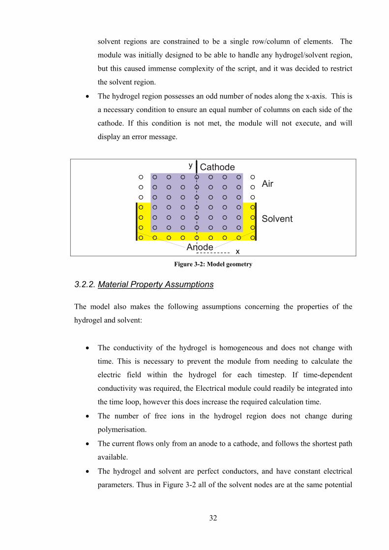
32

solvent regions are constrained to be a single row/column of elements. The

module was initially designed to be able to handle any hydrogel/solvent region,

but this caused immense complexity of the script, and it was decided to restrict

the solvent region.

• The hydrogel region possesses an odd number of nodes along the x-axis. This is

a necessary condition to ensure an equal number of columns on each side of the

cathode. If this condition is not met, the module will not execute, and will

display an error message.

OOOOOOOOO

OOOOOOOOO

OOOOOOOOO

OOOOOOOOO

OOOOOOOOO

OOOOOOOOO

OOOOOOOOO

OOOOOOOOO

OOOOOOOOO

OOOOOOOOO

OOOOOOOOO

OOOOOOOOO

OOOOOOOOO

OOOOOOOOOCathode

Anode

Air

Solvent

Figure 3-2: Model geometry

3.2.2. Material Property Assumptions

The model also makes the following assumptions concerning the properties of the

hydrogel and solvent:

• The conductivity of the hydrogel is homogeneous and does not change with

time. This is necessary to prevent the module from needing to calculate the

electric field within the hydrogel for each timestep. If time-dependent

conductivity was required, the Electrical module could readily be integrated into

the time loop, however this does increase the required calculation time.

• The number of free ions in the hydrogel region does not change during

polymerisation.

• The current flows only from an anode to a cathode, and follows the shortest path

available.

• The hydrogel and solvent are perfect conductors, and have constant electrical

parameters. Thus in Figure 3-2 all of the solvent nodes are at the same potential

x

y

33

as the anode and the solvent acts as one “C-shaped” electrode. The height of

this electrode is dependent on the volume of solvent used.

• Any node in the system that is in direct contact with an electrode is at the same

potential as that electrode.

• Double-layer effects are considered to be negligible in comparison to the voltage

of the electrodes, and the Donnan theory is assumed to be valid. Double-layer

effects result from the build up of charged ions at the electrode/solvent interface.

This effect results in a slight voltage drop occuring at the interface, and so the

actual voltage is lower than the indicated voltage. The Donnan potential of a

hydrogel does change under the influence of an external electric field, but in this

work this change is assumed to be small. This thinking is similar to that

discussed by Shiga [68] who showed that under the influence of an electric field,

the perturbation of the Donnan potential from equilibrium was very small, and

could be ignored. This is contrary to results published by Gong et al. [53]

however, who showed that a large potential drop occurred at the

electrode/hydrogel interface. It is hoped that future work will clarify the

importance of the issues, and either include or exclude them from this model.

• The solvent ions are evenly distributed throughout the solvent regions, and the

ion concentration can be considered homogeneous.


In order to model the electrical field distributions in the hydrogel and solvent regions,

one has to solve the appropriate governing equations subject to some initial and

boundary conditions.

3.3.1. Initial Voltage Distribution

Most of the difficulties in calculating the electric field arise from different anode and

cathode geometries which can be readily overcome by assuming a specific geometry (as

discussed in section 3.2). The basis for the calculation of the electric field stems from

Maxwell’s equations, which in free space can be expressed as [101]:

0

ρε

∇ ⋅ =E (3.1)

0∇ ⋅ =B (3.2)

34

t∂

∇× = −∂BE (3.3)

0 0 0 tµ ε µ ∂

∇× = +∂EB J (3.4)

where E is the electric field intensity, ρ is the charge density, ε0 is the permittivity of

free space, B is the magnetic flux density and J is the vector current density. In an

electrical conductor, there also exists a linear relationship between the vector current

density (J) and electric field intensity (E), namely:

σ=E J (3.5)

where σ is the resistivity of the material. Equation (3.5) is known as Ohm’s Law, and

generally holds only for certain voltage ranges (i.e. it breaks down in the presence of

large potential differences).

The electric field (E) is also defined in terms of the gradient of the scalar voltage

potential, φ , by:

φ= −∇E (3.6)

which allows equation (3.1) to be rewritten as:

( )0

ρφε

∇ ⋅ −∇ = (3.7)

or,

( )0

2

0

ρφερφε

∇ ⋅ ∇ = −

∇ = − (3.8)

where x y z∂ ∂ ∂

∇ = + +∂ ∂ ∂

. Equation (3.8) is known as Poisson’s equation, and occurs in

many different fields of physics.

35

In two dimensions, Poisson’s equation can be written as:

2 2

2 20x y

φ φ ρε

∂ ∂+ =

∂ ∂ (3.9)

In any conductor, ρ is always equal to zero and equation (3.9) is consequently also zero

(Laplace’s equation). Both Poisson’s and Laplace’s equations are a consequence of

conservation of flux. To illustrate how Laplace’s equation is applicable to this work,

consider a point (node) in the hydrogel, labelled as P and surrounded by nodes 1, 2, 3

and 4 (as shown in Figure 3-3).

Figure 3-3: System of connected nodes

For the case shown in Figure 3-3 with ρ=0, equation (3.9) can be written as [102]:

2 2

2 2x yφ φ∂ ∂= −

∂ ∂ (3.10)

If the potential of each node is assumed to be φi, then equation (3.10) can be written as:

( ) ( ) ( ) ( )1 3 2 4P P P Px x y yx y

φ φ φ φ φ φ φ φ− − ∆ + − ∆ − ∆ − − ∆⎛ ⎞ ⎛ ⎞≈ −⎜ ⎟ ⎜ ⎟∆ ∆⎝ ⎠ ⎝ ⎠

(3.11)

where the equality has been replaced by an approximation in light of the discrete spatial

differences introduced. If ∆x = ∆y, equation (3.11) can readily be simplified to give:

1 2 3 4 4 0Pφ φ φ φ φ+ + + − ≈ (3.12)

36

In electrical circuit theory, Laplace’s equation manifests itself as Kirchoff’s current law

(KCL), which states that the sum of currents (i) into and out of each node must equal

zero [103], or:

0i =∑ (3.13)

Using Ohm’s law, the current (i) can be written as:

Rφ∆

=i (3.14)

where ∆φ is the potential difference and R is the electrical resistance. The electrical

resistance is equal to L Aσ , where L is the length and A is the area. Equation (3.13)

may then be written as:

31 2 4 0PP P P

R R R Rφ φφ φ φ φ φ φ−− − −⎛ ⎞⎛ ⎞ ⎛ ⎞ ⎛ ⎞+ + + =⎜ ⎟ ⎜ ⎟ ⎜ ⎟⎜ ⎟

⎝ ⎠ ⎝ ⎠ ⎝ ⎠⎝ ⎠ (3.15)

This is the main governing equation for the field distribution. If the resistance is

assumed to be constant throughout the material, equation (3.15) reduces to:

1 2 3 4 4 0Pφ φ φ φ φ+ + + − = (3.16)

which is identical to equation (3.12). Therefore in the Electrical module, Kirchoff’s

current law will be used as an equivilant to Laplace’s equation.

3.3.2. Boundary Conditions

Boundary conditions are an essential part of any model, and the Electrical module is no

different. The most difficult problem associated with the system described by Figure

3-2 are the air/hydrogel boundaries, as shown in Figure 3-4.

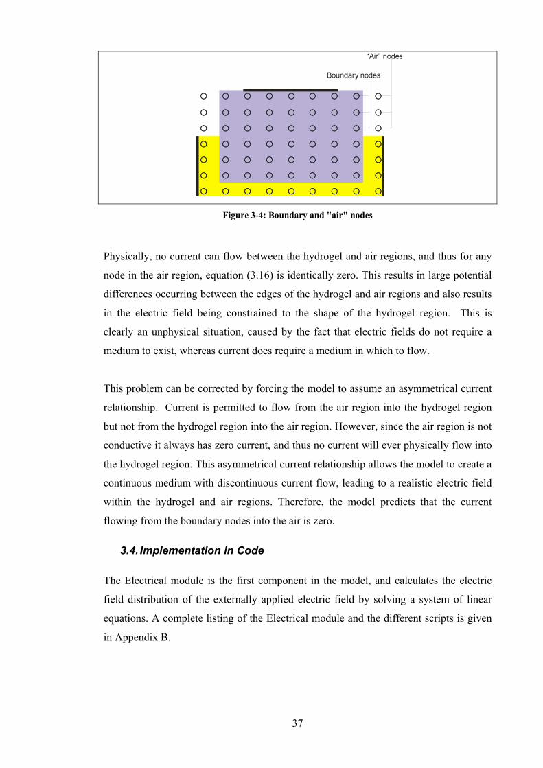
37

OOOOOOOOO

OOOOOOOOO

OOOOOOOOO

OOOOOOOOO

OOOOOOOOO

OOOOOOOOO

OOOOOOOOO

OOOOOOOOO

OOOOOOOOO

OOOOOOOOO

OOOOOOOOO

OOOOOOOOO

OOOOOOOOO

OOOOOOOOO

Boundary nodes

“Air” nodes

Figure 3-4: Boundary and "air" nodes

Physically, no current can flow between the hydrogel and air regions, and thus for any

node in the air region, equation (3.16) is identically zero. This results in large potential

differences occurring between the edges of the hydrogel and air regions and also results

in the electric field being constrained to the shape of the hydrogel region. This is

clearly an unphysical situation, caused by the fact that electric fields do not require a

medium to exist, whereas current does require a medium in which to flow.

This problem can be corrected by forcing the model to assume an asymmetrical current

relationship. Current is permitted to flow from the air region into the hydrogel region

but not from the hydrogel region into the air region. However, since the air region is not

conductive it always has zero current, and thus no current will ever physically flow into

the hydrogel region. This asymmetrical current relationship allows the model to create a

continuous medium with discontinuous current flow, leading to a realistic electric field

within the hydrogel and air regions. Therefore, the model predicts that the current

flowing from the boundary nodes into the air is zero.


The Electrical module is the first component in the model, and calculates the electric

field distribution of the externally applied electric field by solving a system of linear

equations. A complete listing of the Electrical module and the different scripts is given

in Appendix B.

38

The Electrical module is executed from the main control program by calling the script

efield.m. The Electrical module has three variants, which are each related to a different

electrode configuration (Figure 3-5).

OOOOOOOOO

OOOOOOOOO

OOOOOOOOO

OOOOOOOOO

OOOOOOOOO

OOOOOOOOO

OOOOOOOOO

OOOOOOOOO

OOOOOOOOO

OOOOOOOOO

OOOOOOOOO

OOOOOOOOO

OOOOOOOOO

OOOOOOOOOCathode

Anode

(a)

OOOOOOOOO

OOOOOOOOO

OOOOOOOOO

OOOOOOOOO

OOOOOOOOO

OOOOOOOOO

OOOOOOOOO

OOOOOOOOO

OOOOOOOOO

OOOOOOOOO

OOOOOOOOO

OOOOOOOOO

OOOOOOOOO

OOOOOOOOOCathode

Anode

(b)

OOOOOOOOO

OOOOOOOOO

OOOOOOOOO

OOOOOOOOO

OOOOOOOOO

OOOOOOOOO

OOOOOOOOO

OOOOOOOOO

OOOOOOOOO

OOOOOOOOO

OOOOOOOOO

OOOOOOOOO

OOOOOOOOO

OOOOOOOOOCathode

Anode

(c )

Figure 3-5: Different hydrogel/solvent geometries

The three variants of efield.m differ from each other in the following ways:

• efield1.m (Figure 3-5a) assumes that once the hydrogel is placed into the

solvent, it completely displaces all the solvent and as a result no solvent is

present under the hydrogel. This is justified because in reality, the gel could

displace the solution at the bottom surface.

• efield2.m (Figure 3-5b) assumes that the hydrogel does not completely displace

all of the solvent, and as a result there still exists a thin, continuous layer of

solvent underneath the hydrogel. This is case where the weight of the hydrogel

may not completely displace the solvent from the bottom surface.

• efield3.m (Figure 3-5c) utilises a cathode that almost completely covers the top

surface of the hydrogel (as opposed to efield1.m and efield2.m which utilise a

“needle-type” cathode).

39

In this work, the term “efield.m” will be used when referring to elements common to all

three variants. All three involve the use of “air” regions, which are the unshaded nodes

to the sides of the hydrogel region (Figure 3-4). During operation, the Electrical module

runs the following three steps:

Step 1

When called, the Electrical module first sets up a number of different matrices and

vectors required by different parts of the script. By using the assumptions discussed in

section 3.2, efield.m is able to build a complete picture of the hydrogel/solvent/air

system.

Five variables are passed to efield.m – the x- and y-dimensions (in nodes) of the

hydrogel region; the potentials of the anode and cathode, and the level of the solvent.

Because all of the solvent nodes are at the same potential, the model is able to

approximate the solvent as two single columns of nodes on each side of the hydrogel

with or without a single row of nodes underneath the hydrogel (efield1.m or efield2.m,

respectively).

Because of symmetry, efield.m is only required to calculate the voltage potentials for

one half of the hydrogel/solvent/air system, which are then mirrored onto the other side.

This dramatically reduces calculation time, while not adversely affecting the

calculations. An example of this symmetry can be seen in Figure 3-6, which uses

efield2.m.

OOOOOOOOO

OOOOOOOOO

OOOOOOOOO

OOOOOOOOO

OOOOOOOOO

OOOOOOOOO

OOOOOOOOO

OOOOOOOOO

OOOOOOOOO

OOOOOOOOO

OOOOOOOOO

OOOOOOOOO

OOOOOOOOO

OOOOOOOOO

Figure 3-6: Symmetry around y-axis

40

In order to use symmetry however, the Electrical module needs to generate a new

variable that represents the half-width of the gel. efield.m creates the variable, gel_half

which is defined as:

__2

gel xgel half ceiling ⎛ ⎞= ⎜ ⎟⎝ ⎠

(3.17)

where ceiling is defined as the nearest integer to x rounded towards positive infinity.

Thus, in Figure 3-6 gel_half would be equal to 5.

Step 2

Once the Electrical module has set up the different system matrices and vectors, it

begins to set up the system of linear equations that will be solved to provide the voltage

distribution. In order for this to occur, each node in the system is classified dependent

on its position within the hydrogel/solvent system. Individual nodes are labelled as Vn

and specific columns in the hydrogel/solvent system are labelled as C-n, as shown in

Figure 3-7.

Figure 3-7: Numbering of nodes

One interesting feature of the Electrical module is that only nodes with unknown

voltage potentials are calculated (with those potentials known a priori being used to

calculate the unknowns). This is necessary due to the inherent rounding errors present

during numerical modeling that cause deviation from given values. Thus, the anode may

be at a constant voltage of 1V, whereas if calculated by the Electrical module the value

may fall to 0.998V. While these errors are minor in themselves, the compounding

nature of rounding errors makes this problem potentially quite large.

C-1: First column of nodes

C-2: Second column of nodes

C-G: General column of nodes (may consist

of multiple columns)

C-aC: Column adjacent to centre column

C-C: Column of nodes in centre of gel

41

To better illustrate the operation of the Electrical module, an example using efield2.m

will be used. Consider node V14 in Figure 3-7, with a close-up showing the current

flowing into and out of that node shown in Figure 3-8. As mentioned before, the model

assumes that current always flows from the anode to the cathode, and thus the direction

of the arrows is as shown. If the anode and cathode were swapped, the arrows in Figure

3-8 would point in the opposite directions.

V14V13 V15

V9

V19

Figure 3-8: Implementation of Laplace's Equation on node 14

To implement the KCL equation for node 14, equation (3.15) is used. This gives:

15 14 9 14 14 13 14 19V V V V V V V VR R R R− − − −⎛ ⎞ ⎛ ⎞ ⎛ ⎞ ⎛ ⎞+ = +⎜ ⎟ ⎜ ⎟ ⎜ ⎟ ⎜ ⎟

⎝ ⎠ ⎝ ⎠ ⎝ ⎠ ⎝ ⎠ (3.18)

If the resistance is assumed to be constant throughout the hydrogel, then equation (3.18)

becomes:

9 13 14 15 194V V V V V φ− − + − − = (3.19)

which in general form is written as:

4up left n right downV V V V V φ− − + − − = (3.20)

where Vup, Vdown, Vright and Vleft are the voltages at the nodes above, below and to the

right and left of the node currently being examined. Usually φ = 0 in equation (3.20),

but if the specified node was directly adjacent to a node of known potential, Vup (or a

42

similar variable in equation (3.20)) would equal that potential. In this case, φ would be

non-zero for that node.

The Electrical module sets up a matrix of simultaneous equations by iteratively forming

the equivalent KCL equation for each node in the system not known a priori. This

yields n equations (n=29 for Figure 3-8) with the exact form of equation (3.20) being

dependent on both x and y coordinates of the node being examined.

Using these coordinates, the Electrical module classifies each node into a specific type

(for example, a boundary node). Here the advantages of using a constrained geometry

(discussed earlier) become apparent, as the number of possible node types is constrained

and is not dependent on the size of the system. The first variant (efield1.m) of the

Electrical module classifies each node into one of 24 types; the second variant

(efield2.m) into one of 28 types; the third variant (efield3.m) into one of 22 types. The

difference in the number of node types between variants is due to the differing electrode

configurations.

In general, the columns in the hydrogel region (Figure 3-7) are classified as:

• first column of system (C-1)

• second column of system (C-2)

• general columns (C-G)

• column adjacent to centre column (C-aC)

• centre column (C-C).

Within each of these categories, the Electrical module also classifies the node type

dependent on the y-coordinate (row), which are discussed in more detail below:

First column: C-1 nodes

The first (C-1) column of nodes (Figure 3-7) in the system consists of nodes in the air

and solvent regions of the system (nodes V1, V7, V12, V17).

All C-1 nodes have a coefficient of zero for the Vleft potential in equation (3.20) and can

be classified into three possible row types - “first row” (V1), “row above solvent” (V17)

and “generic row” (V11).

43

The “first row” node differs from the “generic row” nodes by the lack of an upwards

current path from the node (i.e. the coefficient of Vup is zero). Also, since the solvent

region is assumed to be at the same potential as the anode, the “row above solvent”

node has φ=Vanode in equation (3.20) and a zero coefficient for the Vdown node. The

remaining nodes are all classified as “generic” nodes and the Laplace equation takes on

the general form shown in equation (3.20).

Second column: C-2 nodes

The second (C-2) column of nodes (Figure 3-7) is the first column in the hydrogel

region. As previously discussed, current can flow into this region from the air region,

but is prevented from flowing out of the hydrogel region into the air region.

Mathematically, this is accomplished by setting the coefficient of Vleft in equation (3.20)

equal to zero for all C-2 nodes.

C-2 nodes can be broken down into five possible types: “first row” (V2), “row above

solvent” (V18), “solvent row” (V22), “last row” (V26) and “generic row” (V13).

Depending on the variant of efield.m that is used, the equations for each node differ

slightly. For the case where efield2.m is used, the C-2 “first” and “generic” nodes are

identical to their C-1 counterparts, with the “first” node having a zero coefficient for

Vup. Since the “solvent row” nodes are adjacent to the anode potential, the value of φ in

equation (3.20) is equal to Vanode (similar to the C-1 “row above solvent” node). The C-

2 “row above solvent” node differs from the C-1 “row above solvent” node in that the

coefficient of Vdown is not zero, which allows an extra current path from this node. The

C-2 “last row” node differs from all the other nodes in this system, in that it is the only

node with 2 current paths to the anode, and also has a zero coefficient for Vdown. For

the C-2 “last row” node, equation (3.20) becomes:

27 26 22 26 26 26

22 26 27

OR4 2

anode anode

anode

V V V V V V V V

V V V V

− + − = − + −

− + − = (3.21)

44

General columns: C-G nodes

General (C-G) nodes (Figure 3-7) are nodes that do not fulfil the criteria for any of the

other four types of nodes in the system, and for this reason the majority of nodes are of

this type. As with the C-2 nodes, there are five possible types of C-G nodes: “first row”

(V3), “row above solvent” (V19), “solvent row” (V23), “last row” (V27) and “generic

row” (V14). In general, these nodes have similar characteristics to their equivalent C-1

and C-2 nodes (i.e. the coefficient of Vtop is equal to zero for “first row” nodes, the

coefficient of Vbot is equal to zero for “last row” nodes) and so will not be repeated for

brevity.

Column adjacent to centre: C-aC nodes

The nodes (Figure 3-7) in the column adjacent to the centre column (C-aC) are almost

identical to the general column (C-G) nodes, and follow the same classification: “first

row” (V4), “row above solvent” (V20), “solvent row” (V24), “last row” (V28) and

“generic row” (V10). In efield2.m, the only difference between the C-G and C-aC

nodes occurs with the “first row” node which has φ in equation (3.20) equal to Vcathode.

Centre column: C-C nodes

The centre column nodes (Figure 3-7) are different from all of the other node types

already discussed. This is because although symmetry does allow the model to only deal

with half of the system, equation (3.20) must still account for the entire system. Again,

for the case of efield2.m, the Centre column (C-C) nodes can be classified as: “second

row” (V11), “row above solvent” (V21), “solvent row” (V25), “last row” (V29) and

“generic row” (V16).

When using efield2.m, the major difference between the C-C “first row” nodes and

other nodes is that the coefficients of Vleft, Vright, Vup and Vdown are all zero. From the

potential of the “first row”, the “second row” node also differs from the “generic” nodes

of other columns, and φ in equation (3.20) is equal to Vcathode. In order to compensate for

the discarded half of the system, the model assumes that the current flux in the negative-

x direction (towards the left in Figure 3-9) is equal to the current flux in the positive-x

direction (right).

45

V7

V11

V17

V12

Figure 3-9: Using the centre column to account for symmetry

Thus, from Figure 3-9 it can be seen that the coefficient of Vright is zero, while the

coefficient of Vleft is equal to 2. Aside from these differences, the “row above solvent”,

“solvent row”, “last row” and “generic row” nodes are identical to those for the C-G

nodes.

By iteratively forming the KCL equations for each node in the system, the Electrical

module builds up a series of simultaneous equations (Figure 3-10) that MATLAB can

then solve. The main difficulty is ensuring that each node in the system is classified

correctly, as an incorrect classification will lead to the incorrect form of KCL equation

being used.

Node 1: 1 2 3 42 0 0 0V V V V+ + + =

Node 2: 1 2 3 40 0 0 anodeV V V V V+ + + =

Node 3: 1 2 3 40 0 cathodeV V V V V+ + + =

Figure 3-10: Simultaneous KCL equations

Step 3

Once the equations for each node have been calculated, the Electrical module then

assembles them into a global node matrix as shown in equation (3.22).

4

011 2 0 020 1 0 0

0 0 1 1

anode

cathode

VVV

VV

⎛ ⎞⎛ ⎞⎛ ⎞⎜ ⎟⎜ ⎟⎜ ⎟⎜ ⎟⎜ ⎟⎜ ⎟ =⎜ ⎟⎜ ⎟⎜ ⎟⎜ ⎟⎜ ⎟⎜ ⎟

⎝ ⎠⎝ ⎠ ⎝ ⎠

(3.22)

46

The system of simultaneous equations in (3.22) can be solved by MATLAB to give the

voltage potentials Vn of each of the nodes. One possible problem with using this method

is that if the coefficient matrix in equation (3.22) is a sparse matrix, MATLAB cannot

solve the system accurately. However, in this case MATLAB would display an error

message with details concerning the accuracy of the returned results, which a user could

then compensate for.

Once equation (3.22) has calculated the voltage potentials of each of the nodes in the

system, the Electrical module combines these values with those potentials known a

priori and returns the entire voltage potential matrix (Figure 3-11) to the main control

program.

5 5 5 5 5 5 5 5 5 5 55 4.7871 4.6592 4.5833 4.5396 4.5245 4.5396 4.5833 4.6592 4.7871 55 4.4892 4.2662 4.1344 4.0506 4.0189 4.0506 4.1344 4.2662 4.4892 5

4.1772 3.9035 3.7821 3.6376 3.5096 3.4498 3.5096 3.6376 3.7821 3.9035 4.17723.6282 3.4391 3.3212 3.1242 2.9004 2.761 2.9004 3.1242 3.3212 3.4391 3.62823.2682 3.0926 2.9394 2.6375 2.2068 1.7936 2.2068 2.6375 2.9394 3.0926 3.26823.0838 2.8994 2.7061 2.2797 1.4955 0 1.4955 2.2797 2.7061 2.8994 3.0838

Figure 3-11: Matrix of voltage potentials, with Vanode=5 and Vcathode=0

The main purpose for calculating the voltage potential matrix is to enable the main

control program to calculate the electric field present within the hydrogel region (Egel).

The module also returns pseudo-values for the air regions (shaded areas in Figure 3-11),

but as previously mentioned, these are not used by the model, and are discarded.

From equation (3.6), it can be seen that the electric field is equal to the negative gradient

of the potential field. This is calculated in MATLAB using the numerical gradient

(gradient.m), which uses a centred-difference method and one-sided differences at the

edges of the matrix. A flowchart of the operation of efield.m is shown in Figure 3-12.

47

Set up system matrices & vectors

For i=1 to number of

nodes

Determine type of node

First column of system nodes

First column of gel nodes

Column next to Centre column

nodes

Centre column nodes

General column nodes

Assemble and solve matrices

All nodes processed?

Return to MAIN

NO

YES

Constants from MAIN

Figure 3-12: Flowchart of efield.m

48

4. Chemical Module

4.1. Introduction

The Chemical module is the second module in the overall model. It calculates the

material flux within the gel/solvent system and the change in ion concentrations

throughout the polymer and solvent regions. The change in ion concentrations is then

used by the Force module to calculate the forces on the hydrogel. These forces are then

passed to the Mechanical module, which calculates the deformation of the hydrogel

region. The Chemical module is also the first module inside the time loop and it takes

information from the previous timestep concerning the spatial ion concentrations in the

gel and solvent regions.

The main inputs into this module are:

• Information concerning the chemical nature of the system (including ion

concentrations, diffusion coefficients and other thermodynamic constants).

• Information on the externally-applied and intrinsic electric fields (resulting from

the charge of the different ions) generated by the Electrical module.

• Information on the geometry and operational controls of the system (including

information on global nodes/elements and timestep values used for time-

integration).

The outputs of this module are the spatial concentrations of all ions in the system as

well as the temporal change in ion concentrations (Figure 4-1).

Figure 4-1: Position of Chemical module in overall model

49

The hydrogel used in this work consists of partially neutralised poly(acrylic acid)

(PAAC), which partially dissociates (based on the pH during the gel formation) to leave

negatively charged COO- groups attached to the polymer backbone and positive mobile

counterions (Na+) in the hydrogel. The gel is placed into an aqueous NaCl solution,

which is assumed to be completely dissociated, containing an excess of ions. This

solvent provides a source of mobile Na+ and Cl- ions (as illustrated in Figure 4-2).

COO-

Cl-

Cl- Cl- Cl- Cl- Cl-Na+ Na+ Na+ Na+ Na+ Na+

Na+Na+

Na+

GEL

SOLVENTCOO-

COO-

Figure 4-2: Ion concentration in gel and solvent regions

The Chemical module treats the charged ions in the system as three separate species –

mobile Na+ ions, mobile Cl- ions and stationary COO- ions (present in the hydrogel

region). It calculates the mass transport of these three ions based on diffusion and

migration under the influence of an externally-applied electric field to provide spatial

and temporal information on the change in ion concentrations.

4.2. Assumptions

In developing the Chemical module, the following assumptions are made:

• The different ionic species do not interact physically with each other, and could

therefore theoretically occupy the same region of space. While this assumption

generally only holds for very low ionic concentrations, it does simplify the

required calculations and so is used in this module. The module does consider

electrostatic interactions between different ionic species however, and this

prevents like ions from occupying the same regions of space

• The initial concentrations of ions present in the system do not change (i.e. the

Chemical module does not consider dissociation/recombination reactions, which

greatly increase the complexity of the model). This allows the model to

calculate the initial ion concentration distributions and evolve these steadily

through time.

• The charges on the polymer backbone are unable to move, and thus do not

change in position. In reality, the polymer chains can deform and this does

50

provide some mobility to the stationary COO- ions. The stationary COO- ions do

interact with the other species in the system through electrostatic interactions.

• There is an excess of Na+ and Cl- ions in the solvent surrounding the hydrogel,

and thus there is no change in concentration as ions move into or out of the

solvent region.

• The system is at constant temperature and pressure.


The theoretical development of the Chemical module is divided into two main parts:

1) Determination of the initial ion concentrations for ions in the solvent and

hydrogel regions.

2) Determination of the mass transport equations for each ionic species in the

model.

4.3.1. Initial Ion Concentrations

The solvent surrounding the hydrogel consists of an aqueous solution of NaCl salt,

which by definition completely dissociates into an equal number of Na+ and Cl- ions.

The concentration of these ions in the solvent region is easily calculated from

knowledge of the salt concentration used in the preparation of the solvent (i.e. 1mol of

NaCl dissolved into 1L would provide a concentration of 1 mol L-1). These ions are

assumed to be distributed evenly throughout the solvent region, and available in excess

so that their concentration remains essentially constant.

Calculation of the initial ion concentrations in the hydrogel region is slightly more

involved, and requires knowledge of both the pre-gel concentrations and preparation

conditions. Hydrogels are known to be heterogeneous in structure [104], which makes it

difficult or impossible to accurately describe the charge distribution within the

hydrogel. Counterions are known to play the main role in electrical conduction, and the

appearance of periodic current variations is a direct feature of the crosslinked nature of

polymer hydrogels. Osada et al. [104] states that the speed of deformation is dependent

only on the amount of charge being transported and not on the applied field, but this in

direct contradiction to Salehpoor et al. [66] who showed a speed dependence on the

magnitude of the applied electric field. The polymer hydrogel used in this work is

formed from partially-neutralised acrylic acid (AAC), a weak acid with an ionisable

51

carboxy group (Figure 4-3) that provides the stationary COO- groups found in the

hydrogel.

C

C C

O

O HH

H

H

Figure 4-3: Acrylic Acid monomer

Using the acid dissociation constant (Ka), the Chemical module calculates the initial

concentration of COO- and Na+ ions in the hydrogel region. This is discussed in more

detail in chapter 7.

Unlike ions in the solvent region, ions in the gel region are not assumed to be uniformly

distributed. While an even distribution of ions is sometimes assumed to exist in the

hydrogel region (similar to the distribution of the solvent ions), it is well known that in

poly(acrylic acid) hydrogel, spatial inhomogeneities exist [105] and that “clusters” of

ions form within the hydrogel. Therefore, to distribute the ions within the hydrogel

region, the overall model considers two types of electrostatic interactions: Coulombic

and Lennard-Jones.

Coulombic interactions are considered fundamental, and occur between all charged

particles in nature. The Coulombic potential energy between a pair of point charges is

defined as [106]:

0

14

i jc

ij

v vU

rπε= (4.1)

where vi is the valence of the ith ion and rij is the distance between the two ions.

Equation (4.1) describes the interactions between particles in free space, and generally

does not hold when considering real materials. In particular, polyelectrolyte hydrogels

consist of a large number of charges which are confined (by the geometry of the

material) to be in close proximity to each other. In this case, one must also consider

52

effects such as Manning condensation [107], whereby charges “condense” onto the

polymer backbone and decrease the amount of apparent charge present. The limiting

factor for this occurs when the charge density within the polyelectrolyte exceeds one

charge per Bjerrum length, Bλ , which is given by [108]:

2

04Br B

ek T

λπε ε

= (4.2)

where ε0 and εr are the permittivity of free space and the solvent respectively, kB is the

Boltzmann constant and T is the temperature. As a result of Manning condensation, the

Coulombic potential energy within polyelectrolyte hydrogels may be written as [109]:

i jc B B

ij

v vU k T

rλ= (4.3)

which is the definition that will be used in this work to distribute the COO- and Na+ ions

within the hydrogel region.

Particles also interact via a Lennard-Jones (L-J) potential of the form [110], which

amongst other things prevents any two ions from occupying the same region of space.

12 6

( ) 4ij ijU rr rσ σε

⎡ ⎤⎛ ⎞ ⎛ ⎞= −⎢ ⎥⎜ ⎟ ⎜ ⎟⎝ ⎠ ⎝ ⎠⎢ ⎥⎣ ⎦

(4.4)

where σ is the molecular separation and εij is the depth of the potential well. The L-J

potential in this work acts predominantly as a repulsive force (since most of the

attractive/repulsive force stems from the Coulombic interaction). Since the polymer

hydrogel consists mainly of water, the model uses the values of water for σ, εij and εr.

53

4.3.2. Determination of the Mass Transport Equations

In order to calculate the mass transport equations for the ionic species present in the

system, it is necessary to examine the fundamental mechanisms responsible for mass

transport.

The second law of thermodynamics states that any system initially not in equilibrium

will always move towards a state of equilibrium, and the changes that occur to the

system are generally considered to be irreversible. For a closed system to be in

equilibrium, the entropy of the system (S) must be maximal [111]. Therefore, the

entropy of the system should not vary as the energy, volume or number of particles

changes, or:

1 1 2 2

1 1 2 2

1 1 22

1 21

1 2, ,

1 21

1 2, ,

1 21

1 2, ,

0

V N V N

E N E N

V E V E

S SdS dEE E

S S dVV V

S S dNN N

⎡ ⎤⎛ ⎞ ⎛ ⎞∂ ∂⎢ ⎥= −⎜ ⎟ ⎜ ⎟∂ ∂⎢ ⎥⎝ ⎠ ⎝ ⎠⎣ ⎦⎡ ⎤⎛ ⎞ ⎛ ⎞∂ ∂⎢ ⎥+ −⎜ ⎟ ⎜ ⎟∂ ∂⎢ ⎥⎝ ⎠ ⎝ ⎠⎣ ⎦⎡ ⎤⎛ ⎞ ⎛ ⎞∂ ∂⎢ ⎥+ −⎜ ⎟ ⎜ ⎟∂ ∂⎢ ⎥⎝ ⎠ ⎝ ⎠⎣ ⎦

=

(4.5)

where S is the entropy, iE is the energy, iV is the volume and iN is the number of

particles in region i. In a system that is at constant temperature, pressure and volume,

the first two terms are easily satisfied. For particle equilibrium (equal particle density in

all regions in the system), the entropy of the system must not change when changing the

number of particles. In other words:

1 1 2 2

1 2

1 2, ,E V E V

S SN N

⎛ ⎞ ⎛ ⎞∂ ∂=⎜ ⎟ ⎜ ⎟∂ ∂⎝ ⎠ ⎝ ⎠

(4.6)

54

In electrochemistry it is usually more convenient to use the chemical potential, iµ ,

which is defined as:

,i i

ii i

i E V

ST

Nµ

⎛ ⎞∂= ⎜ ⎟∂⎝ ⎠

(4.7)

where Ti is the temperature of the system. Using equation (4.7), and assuming constant

temperature and pressure, equation (4.6) may be rewritten as:

1 2µ µ= (4.8)

Equation (4.7) can also be rewritten with different thermodynamic variables held

constant, for example the Helmholtz free energy (F) or Gibbs free energy (G):

,T V

FN

µ ∂⎛ ⎞= ⎜ ⎟∂⎝ ⎠ (4.9)

,T P

GN

µ ∂⎛ ⎞= ⎜ ⎟∂⎝ ⎠ (4.10)

where P is the pressure and T is the temperature. It is also possible to express other

thermodynamic variables in terms of the chemical potential. For example, the volume

is also given by:

,T N

VPµ∂⎛ ⎞= ⎜ ⎟∂⎝ ⎠

(4.11)

To relate the chemical potential to the activity (and concentration) of a species, consider

an ideal gas.

55

Using equation (4.11) in combination with the ideal gas law, one can derive an equation

for the chemical potential at a point r ( ( , , )r x y z=r ) in the system [112]:

[ ]0( ) ( ) ln ( )i i iRT aµ µ= +r r r (4.12)

where 0 ( )iµ r and ia are the reference potential and activity of species i, respectively.

The activity (and more particularly the activity coefficient) relates the concentration of a

species to its actual thermodynamic activity, and in practice has limited use. For low

concentrations however (<1 mol L-1), the activity can usually be assumed to be

approximately equal to the concentration (Ci) of species i. Additionally, if there is an

electrostatic potential present in the solution, an extra term must be added to equation

(4.12), to give:

[ ]0( ) ( ) ln ( ) ( )i i i iRT a z Fµ µ φ= + +r r r r (4.13)

where iz is the charge number, ( , )x yφ is the electrostatic potential and R, T and F are

the molar gas constant, temperature and Faraday constant, respectively. In

electrochemical systems, the chemical potential is the main driving mechanism for the

mass transport process.

Flux (J) of species i will occur to alleviate any differences in the chemical potential,

with that flux being proportional to the gradient of the chemical potential:

i iµ∝ ∇J (4.14)

where the r has been dropped for convenience. Experimentally, it was found [113] that

the constant of proportionality is given by:

i iC DRT

γ = − (4.15)

where iC is the concentration of species i and iD is a species-specific “diffusion

coefficient” that is empirically determined. Netz and Dorfmuller [114, 115] performed

Monte Carlo simulations on the path of “tracer” particles to determine the effects of

geometrical obstructions on the diffusion in hydrogels and found for 2-dimensional

56

systems with a moderate concentration of obstacles, the diffusion was anomalous (i.e.

did not obey Fick’s 2nd law) for short distances and was normal over long distances. In

the case of this work, the distances are considered to be large, and so normal diffusion is

assumed to apply.

The negative sign in equation (4.15) results from the fact that flux moves from regions

of higher potential to regions of lower potential. Equation (4.14) can then be written as:

( )0 lni ii i i i

C DRT a z F

RTµ φ⎛ ⎞ ⎡ ⎤= − ∇ + +⎜ ⎟ ⎣ ⎦⎝ ⎠

J (4.16)

The first term in equation (4.16) is constant, and thus its gradient is zero. Considering

only the second term, and using equation (4.15) gives:

[ ]

[ ]

[ ]

, ln( )

ln( )

ln( )

i ii diff i

i ii

i i i

i i

C D RT aRT

C D RT CRT

D C CD C

⎛ ⎞= − ∇⎜ ⎟⎝ ⎠⎛ ⎞≈ − ∇⎜ ⎟⎝ ⎠

= − ∇

= − ∇

J

(4.17)

for each species i, with the activity replaced with the concentration as discussed earlier.

Equation (4.17) is commonly referred to as Fick’s first law of diffusion, and serves to

equilibrate the concentration. Diffusion occurs in all liquids and gases, and is a direct

consequence of the second law of thermodynamics. For systems containing only

neutral species (z=0), equation (4.17) represents the total driving force for mass

transport within the system and for this reason is usually considered to be one of the

most important phenomenon in electrochemistry.

The third term in equation (4.16) is commonly referred to as the migratory flux and can

be written as:

[ ],i i

i mig i

i i i

C Dz F

RTC D z F

RT

φ

φ

⎛ ⎞= − ∇⎜ ⎟⎝ ⎠

= − ∇

J (4.18)

57

Einstein [116] discovered a relationship between the electrolytic mobility (the velocity

of a particle under an electric field of unit strength) of a particle and the diffusion

coefficient (Di), which is described by the Einstein-Smoluchowski (or Nernst-Einstein)

equation:

i ii

z FDU

RT= (4.19)

Substituting equation (4.19) into equation (4.18) gives:

,i

i mig i ii

UC z

zφ= − ∇J (4.20)

Equation (4.20) results from the various species in the system having different

mobilities. By combining equations (4.17) and (4.20), one can derive a general

equation for mass transport in electrochemical systems:

ii i i i i

i

UD C C z

zφ= − ∇ − ∇J (4.21)

which is known as the Nernst-Planck equation. In general, the Nernst-Planck equation

also incorporates a term to describe convection within the system, in which case

equation (4.21) becomes:

ii i i i i i

i

UD C C z C

zφ= − ∇ − ∇ +J v (4.22)

where v is the flow velocity of the surrounding solution. In this work however, it is

assumed that the system is quiescent (i.e. there is no forced convection) and so

convection can be ignored. This allows equation (4.21) to be used in this work.

In order to gain better insight into the gradient of the electrostatic potential, it is

sometimes more useful to describe equation (4.21) in terms of electrical flux, j, instead

of the material flux, Ji.

58

Faraday’s law [113] can be used to relate the electrical and material flux:

i ii

z F= ∑j J (4.23)


ii i i i i i i

i i i

i i i i i ii i

Uz F D C z F C z

z

z FD C F z U C

φ

φ

⎛ ⎞ ⎛ ⎞= − ∇ − ∇⎜ ⎟ ⎜ ⎟

⎝ ⎠ ⎝ ⎠

= − ∇ − ∇

∑ ∑

∑ ∑

j (4.24)

Equation (4.24) can be further simplified by identifying that the conductivity σ is given

by:

1i i i

iz FU C

Rσ = =∑ (4.25)

where R is the electrical resistance. Thus, equation (4.24) becomes:

i i i ii

z FD C σ φ= − ∇ − ∇∑j (4.26)

which can be rearranged into:

i i ii i

z FD Cφ

σ σ

∇∇ = − −

∑ j (4.27)

From (4.27) it can be seen that the electric potential is the sum of two terms. The first

term arises from spatial concentration differences of each ion species i, with differing

charge numbers and is usually referred to as the diffusion potential gradient. The

second term is Ohm’s law, and is the result of an externally imposed voltage gradient on

the system. For this reason, the second term is usually referred to as the ohmic potential

gradient, and is generally larger than the diffusion potential gradient.

59

In order to describe the change in concentration in both time and space, it is necessary

to derive an equation with concentration as a dependent variable, and space and time as

independent variables. Equation (4.21) is useful, but is also spatially dependent and thus

unsuitable in its current form.

In order for equation (4.21) to be of use in this work, it is necessary to describe the

change in concentration as a function of both space and time which can be achieved

using the material flux. In a theoretical region of space bounded by a surface S (Figure

4-4), the change in the amount of physical material, M, as a function of time is related to

the flux (J) across the surface of that region, or:

(4.28)

where the integral is taken over the entire surface S and the normal vector dS points

outwards from the surface.

Figure 4-4: Flux over a surface

M is also related to the change in concentration over time for some volume, dV:

iCM dVt t

∂∂=

∂ ∂∫ (4.29)

Using equations (4.28) and (4.29) the flux, J, can be related to the change in

concentration over time by:

i

V

CdV d

t∂

= − ⋅∂∫ ∫ J S (4.30)

60

The divergence theorem can then be utilised to relate the surface integral to a volume

integral:

V

d dV⋅ = ∇ ⋅∫ ∫J S J (4.31)


iCt

∂= −∇ ⋅

∂J (4.32)

Using equation (4.21) and equation (4.32), one can derive an expression for the spatial

and temporal change in concentration of species i:

2 2i ii i i i i

i

C UD C z C C

t zφ φ

∂⎡ ⎤= ∇ + ∇ +∇ ∇⎣ ⎦∂

(4.33)

Under the assumption of electroneutrality (where the number of positive charges is

equal to the number of negative charges), the Laplacian operator of the potential field is

zero and the second term in (4.33) is zero. Thus, we finally arrive at the governing

equation for the Chemical module, which for each species i is given by:

2i ii i i i

i

C UD C z C

t zφ

∂= ∇ + ∇ ∇

∂ (4.34)

In order to calculate the temporal change in concentration, the Chemical module

implements the two-dimensional equivalent of equation (4.34), which is given by:

2 2

2 2

2 2

1 2 2

1

i i ii

i i ii

i

i i

i i

C C CDt x y

U C Czz x y x y

C Cx y

C Cx y x y

φ φ

α

φ φβ

⎛ ⎞∂ ∂ ∂= +⎜ ⎟∂ ∂ ∂⎝ ⎠

⎛ ⎞⎛ ⎞∂ ∂ ∂ ∂+ + +⎜ ⎟⎜ ⎟∂ ∂ ∂ ∂⎝ ⎠⎝ ⎠

⎛ ⎞∂ ∂= +⎜ ⎟∂ ∂⎝ ⎠

⎛ ⎞⎛ ⎞∂ ∂ ∂ ∂+ + +⎜ ⎟⎜ ⎟∂ ∂ ∂ ∂⎝ ⎠⎝ ⎠

(4.35)

61

where the constants 1α and 1β are introduced for convenience. In order to calculate an

approximate solution to equation (4.35), the Chemical module uses Galerkin’s method

of weighted residual with a forward-difference time-integration scheme. The module

solves equation (4.35) for each species i in the system, and the various species are

assumed not to interact physically (i.e. they could theoretically operate in the same

region of space).

The ions do still interact electrostatically however, and like ions tend to move away

from each other while unlike ions are attracted to each other. As discussed in chapter 2,

the Galerkin method uses the original shape (basis) functions (H1, H2 and H3) of the

elements as a weight function (w), which for linear triangular elements are given by

[99]:

( ) ( ) ( )

( ) ( ) ( )

( ) ( ) ( )

1 2 3 3 2 2 3 3 2

2 3 1 1 3 3 1 1 3

3 1 2 2 1 1 2 2 1

121

21

2

H x y x y y y x x x yA



= − + − + −⎡ ⎤⎣ ⎦

= − + − + −⎡ ⎤⎣ ⎦

= − + − + −⎡ ⎤⎣ ⎦

(4.36)

where H is the shape function, A is the area, and xi and yi are the ith node of each

triangular element. Integration of the weighted residual of equation (4.35) over the

domain Ω and boundary Γ yields:

2 2

2 2

I =

0

Cw dt

C Cw w dx y

C C Cw w d w dx y x y n

α

φ φβ α

Ω

Ω

Ω Γ

∂Ω

∂

⎛ ⎞∂ ∂− + Ω⎜ ⎟∂ ∂⎝ ⎠

⎛ ⎞⎛ ⎞∂ ∂ ∂ ∂ ∂− + + Ω− Γ⎜ ⎟⎜ ⎟∂ ∂ ∂ ∂ ∂⎝ ⎠⎝ ⎠=

∫

∫

∫ ∫

(4.37)

which can be simplified using integration by parts to give the weak form (where no

derivative is greater than first order) of equation (4.37):

62

C w C w CI w d dt x x y y

C C Cw w d w dx y x y n

α

φ φβ α

Ω Ω

Ω Γ

⎛ ⎞∂ ∂ ∂ ∂ ∂= Ω+ + Ω⎜ ⎟∂ ∂ ∂ ∂ ∂⎝ ⎠

⎛ ⎞⎛ ⎞∂ ∂ ∂ ∂ ∂− + + Ω− Γ⎜ ⎟⎜ ⎟∂ ∂ ∂ ∂ ∂⎝ ⎠⎝ ⎠

∫ ∫

∫ ∫ (4.38)

The last term in (4.38) describes the flux normal to the boundary of the system (mass

transport into or out of the system), and for this module presents some interesting

challenges. By examining Figure 4-5 it can be seen that the system consists of three

parts:

(1) a gel submersed in a

(2) surrounding solvent with

(3) air above the solvent and next to the gel.

OOOOOOOOO

OOOOOOOOO

OOOOOOOOO

OOOOOOOOO

OOOOOOOOO

OOOOOOOOO

OOOOOOOOO

OOOOOOOOO

OOOOOOOOO

OOOOOOOOO

OOOOOOOOO

OOOOOOOOO

OOOOOOOOO

OOOOOOOOO

Gel

Solvent

AirFree space

Figure 4-5: Gel and solvent system

Realistically, no material flux can pass through the air regions and thus, these regions

must be isolated from equation (4.38). If these space regions were not isolated and were

given the accurate value of zero (since there are clearly no ions in these regions), ion

transport would occur from the gel or solvent into these regions (since diffusion occurs

from a region of finite concentration to a region of zero concentration). This problem is

overcome in the Chemical module by separating the entire system into two subsystems

that overlap as shown in Figure 4-6.

OOOOOOOOO

OOOOOOOOO

OOOOOOOOO

OOOOOOOOO

OOOOOOOOO

OOOOOOOOO

OOOOOOOOO

OOOOOOOOO

OOOOOOOOO

OOOOOOOOO

OOOOOOOOO

OOOOOOOOO

OOOOOOOOO

OOOOOOOOO

OOOOOOOOO

OOOOOOOOO

OOOOOOOOO

OOOOOOOOO

OOOOOOOOO

OOOOOOOOO

OOOOOOOOO

OOOOOOOOO

OOOOOOOOO

OOOOOOOOO

OOOOOOOOO

OOOOOOOOO

OOOOOOOOO

OOOOOOOOO

OOOOOOOOO

OOOOOOOOO

OOOOOOOOO

OOOOOOOOO

OOOOOOOOO

OOOOOOOOO

OOOOOOOOO

OOOOOOOOO

OOOOOOOOO

OOOOOOOOO

OOOOOOOOO

OOOOOOOOO

OOOOOOOOO

OOOOOOOOO

OOOOOOOOO

OOOOOOOOO

OOOOOOOOO

OOOOOOOOO

OOOOOOOOO

OOOOOOOOO

OOOOOOOOO

OOOOOOOOO

OOOOOOOOO

OOOOOOOOO

OOOOOOOOO

OOOOOOOOO

OOOOOOOOO

OOOOOOOOO

Figure 4-6: System separated into "solvent" and "gel" subsystems

63

This separation of subsystems is similar to that which occurs when a Gibbs ensemble

method is used to model hydrogel swelling, as discussed by Kenkare et al. [75]. In that

case, two simulation cells are used with one cell being for the bulk solvent phase and

one cell being for the gel phase. In this work, these subsystems are referred to as the

“gel” and “solvent” subsystems, and operate independently of each other. As expected,

this method of solving boundary-flux problems generates its own unique difficulties, the

most notable being the extra computational time required to calculate equation (4.38)

multiple times. Since each species in this module is treated independently, the Chemical

module solves equation (4.38) for the concentration of each species i at each node,

resulting in s instances of equation (4.38), where s is the number of species in the

system. Since the entire system is now divided into two subsystems (“gel” and

“solvent”) the number of instances grows to a total of 2s. In our case where there are

two species (Na+ and Cl-), equation (4.38) is solved four times. The solvent system is

calculated first, and this also results in the “gel” subsystem lagging behind the “solvent”

subsystem.

Another major problem with dividing the system into “solvent” and “gel” subsystems is

that while the “gel” subsystem consists solely of elements associated with the gel, the

“solvent” subsystem also has an interface between the hydrogel and surrounding

solvent. To overcome this problem when modeling hydrogel systems, this interface is

treated as a semi-permeable membrane which effects the diffusion of ions into the gel

system. However, since this is the first generation of this model, the gel/solvent

interface is assumed to not noticeably affect the diffusion of ions and water into the gel.

This issue will need to be set aside for future investigation.

The advantage of using the subsystem method however, is that now both subsystems

have zero-flux boundary conditions ( C∂ / 0n∂ = ), which is a consequence of their

independence. Equation (4.38) can then be simplified to:

C w C w CI w d dt x x y y

C Cw w dx y x y

α

φ φβ

Ω Ω

Ω

⎛ ⎞∂ ∂ ∂ ∂ ∂= Ω+ + Ω⎜ ⎟∂ ∂ ∂ ∂ ∂⎝ ⎠

⎛ ⎞⎛ ⎞∂ ∂ ∂ ∂− + + Ω⎜ ⎟⎜ ⎟∂ ∂ ∂ ∂⎝ ⎠⎝ ⎠

∫ ∫

∫ (4.39)

64

which is now an integral over the domainΩ , only. Substituting (4.36) into (4.39) gives:

( )

1

2

3

1

2

3

CA C

C

B+C

D+E

t t

t t

I d

w C w C d Cx x y y

CCd

x y

α

φ φβ

+∆

Ω

+∆

Ω

⎧ ⎫⎪ ⎪= Ω⎨ ⎬⎪ ⎪⎩ ⎭

⎛ ⎞⎛ ⎞⎛ ⎞∂ ∂ ∂ ∂+ Ω⎜ ⎟⎧ ⎫⎜ ⎟⎜ ⎟∂ ∂ ∂ ∂⎝ ⎠ ⎪ ⎪⎜ ⎟⎝ ⎠+ ⎨ ⎬⎜ ⎟⎛ ⎞∂ ∂ ⎪ ⎪⎜ ⎟− + Ω ⎩ ⎭⎜ ⎟⎜ ⎟∂ ∂⎝ ⎠⎝ ⎠

∫

∫ (4.40)

for each element in the subsystem, where nC is the concentration of local node n. The

variables A-E represent the following combinations of shape function derivatives:

[ ]1

2 1 2 3

3

1

2 1 2 3

3

1

2 1 2 3

3

11 2 3

2

3

11

2

3

HHH

Hx

H H H Hx x x x

HxH

H H H H

H

HH H HHx x x

H

HH HH

H

A H H H

B

y

Cy y y y

y

D

Ey

⎡ ⎤⎢ ⎥= ⎢ ⎥⎢ ⎥⎣ ⎦∂⎡ ⎤⎢ ⎥∂⎢ ⎥∂ ∂ ∂ ∂⎡ ⎤⎢ ⎥= ⎢ ⎥⎢ ⎥∂ ∂ ∂ ∂⎣ ⎦⎢ ⎥∂⎢ ⎥⎢ ⎥∂⎣ ⎦⎡ ⎤∂⎢ ⎥∂⎢ ⎥⎢ ⎥ ⎡ ⎤∂ ∂ ∂ ∂

= ⎢ ⎥ ⎢ ⎥∂ ∂ ∂ ∂⎣ ⎦⎢ ⎥⎢ ⎥∂⎢ ⎥∂⎣ ⎦⎡ ⎤

∂ ∂ ∂⎡ ⎤⎢ ⎥= ⎢ ⎥⎢ ⎥ ∂ ∂ ∂⎣ ⎦⎢ ⎥⎣ ⎦⎡ ⎤

∂ ∂⎢ ⎥= ⎢ ⎥ ∂⎢ ⎥⎣ ⎦

2 3Hy y

⎡ ⎤∂⎢ ⎥∂ ∂⎣ ⎦

(4.41)

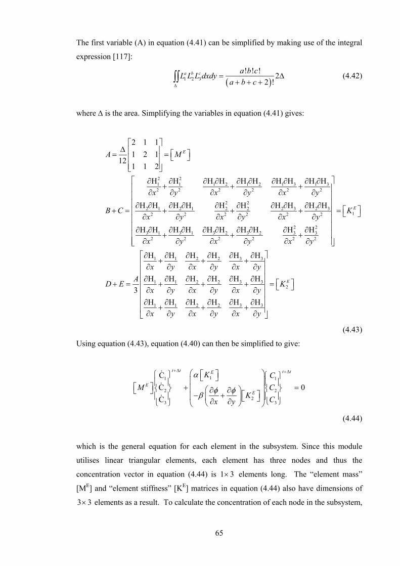
65

The first variable (A) in equation (4.41) can be simplified by making use of the integral

expression [117]:

( )1 2 3! ! ! 2

2 !a b c a b cL L L dxdy

a b c∆

= ∆+ + +∫∫ (4.42)

where ∆ is the area. Simplifying the variables in equation (4.41) gives:

2 21 1 1 2 1 2 1 3 1 32 2 2 2 2 2

2 22 1 2 1 2 2 2 3 2 3

2 2 2 2 2 2

2 23 1 3 1 3 2 3 2 3 3

2 2 2 2 2 2

2 1 11 2 1

121 1 2

H H H H H H H H H H

H H H H H H H H H H

H H H H H H H H H H

EA M

x y x y x y

B Cx y x y x y

x y x y x y

⎡ ⎤∆ ⎢ ⎥ ⎡ ⎤= = ⎣ ⎦⎢ ⎥⎢ ⎥⎣ ⎦⎡ ∂ ∂ ∂ ∂ ∂ ∂ ∂ ∂ ∂ ∂

+ + +⎢ ∂ ∂ ∂ ∂ ∂ ∂⎢⎢∂ ∂ ∂ ∂ ∂ ∂ ∂ ∂ ∂ ∂

+ = + + +⎢∂ ∂ ∂ ∂ ∂ ∂

∂ ∂ ∂ ∂ ∂ ∂ ∂ ∂ ∂ ∂+ + +

∂ ∂ ∂ ∂ ∂ ∂⎣

1

1 1 2 2 3 3

1 1 2 2 3 32

1 1 2 2 3 3

H H H H H H

H H H H H H3

H H H H H H

E

E

K

x y x y x yAD E K

x y x y x y

x y x y x y

⎤⎥⎥⎥

⎡ ⎤=⎥ ⎣ ⎦⎢ ⎥⎢ ⎥⎢ ⎥⎢ ⎥⎦⎡ ⎤∂ ∂ ∂ ∂ ∂ ∂

+ + +⎢ ⎥∂ ∂ ∂ ∂ ∂ ∂⎢ ⎥⎢ ⎥∂ ∂ ∂ ∂ ∂ ∂ ⎡ ⎤+ = + + + =⎢ ⎥ ⎣ ⎦∂ ∂ ∂ ∂ ∂ ∂⎢ ⎥⎢ ⎥∂ ∂ ∂ ∂ ∂ ∂

+ + +⎢ ⎥∂ ∂ ∂ ∂ ∂ ∂⎣ ⎦

(4.43)

Using equation (4.43), equation (4.40) can then be simplified to give:

11 1

2 2

23 3

CC 0C

t t t tE

E

E

K CM C

K Cx y

α

φ φβ

+∆ +∆⎛ ⎞⎡ ⎤⎧ ⎫ ⎧ ⎫⎣ ⎦⎜ ⎟⎪ ⎪ ⎪ ⎪⎡ ⎤ + =⎨ ⎬ ⎨ ⎬⎜ ⎟⎛ ⎞∂ ∂⎣ ⎦ ⎡ ⎤− +⎪ ⎪ ⎪ ⎪⎜ ⎟⎜ ⎟ ⎣ ⎦∂ ∂ ⎩ ⎭⎩ ⎭ ⎝ ⎠⎝ ⎠

(4.44)

which is the general equation for each element in the subsystem. Since this module

utilises linear triangular elements, each element has three nodes and thus the

concentration vector in equation (4.44) is 1 3× elements long. The “element mass”

[ME] and “element stiffness” [KE] matrices in equation (4.44) also have dimensions of

3 3× elements as a result. To calculate the concentration of each node in the subsystem,

66

the “element mass” and “element stiffness” matrices need to be assembled into the

overall “mass” and “stiffness” matrices for each subsystem:

[ ][ ]

[ ]

11 1

2n

C0

C

t t t t

n

K CM

K Cx y

α

φ φβ

+∆ +∆⎛ ⎞⎧ ⎫ ⎧ ⎫⎜ ⎟⎪ ⎪ ⎪ ⎪+ =⎨ ⎬ ⎨ ⎬⎛ ⎞∂ ∂⎜ ⎟− +⎜ ⎟⎪ ⎪ ⎪ ⎪⎜ ⎟∂ ∂ ⎩ ⎭⎝ ⎠⎩ ⎭ ⎝ ⎠

(4.45)

where the concentration vectors C are now 1 n× elements long and the “mass” and

“stiffness” matrices have dimensions n n× , where n is the number of nodes in the

subsystem.

The “element stiffness” matrix [K2E] in equation (4.44) also contains a term describing

the gradient of the electrostatic potential. The two-dimensional equivalent of equation

(4.27) is given by:

1

2

1

si i

i ii i

s

j j jj

C Cz U

x yRTx y F z U C

φ φσ

=

=

∂ ∂⎛ ⎞+⎜ ⎟∂ ∂⎛ ⎞∂ ∂ ⎝ ⎠+ = − − −⎜ ⎟∂ ∂⎝ ⎠

∑

∑j

(4.46)

As discussed previously, the first term in (4.46) results from differences in the

electrolytic mobility of the different ions, while the second term arises from an

externally-applied electric field. Although equation (4.46) contains both an x- and y-

derivative of Ci, it cannot be used directly in equation (4.39). The Chemical module can

only solve the weak form of equation (4.39), and using equation (4.46) directly would

cause the order of the differentiation to increase (thus destroying the weak form of the

equation). This problem can be overcome however, by noting that the first term in

equation (4.46) is small compared to the second term, which is constant. The Chemical

module therefore solves equation (4.46) numerically during each timestep, and uses this

value directly in equation (4.45).

To calculate the time derivative in equation (4.45), the Chemical module uses a

forward-difference time-integration scheme in which the change in concentration is

approximated by the linear function:

67

C CCt t t

t

+∆ −=

∆ (4.47)

This allows equation (4.45) to be simplified to give:

[ ] [ ]( )

[ ]( ) [ ] ( )

C C0 C

C C C

t t tt ti ii

t t t t ti i i

M Kt

M K t

+∆+∆

+∆ +∆

⎛ ⎞−= +⎜ ⎟∆⎝ ⎠

= − + ∆

(4.48)

for each species i, where [K] = [K1]+[K2]. Equation (4.48) can be rearranged to give:

[ ] [ ]( )( ) [ ]( )C Ct t ti iM K t M+∆+ ∆ = (4.49)

where Cti is the concentration of the nodes at the previous timestep. The forward-

difference method is ideal for calculating the concentration of the nodes at the following

timestep, since by default, the initial concentration 0Ci of all of the nodes is known.


The Chemical module can be broken down into three separate parts – two of these parts

are responsible for generation of the initial system conditions (and occur outside of the

time loop), while the third is used to calculate the change in ion concentrations

throughout the gel/solvent region. A complete listing of the Chemical module and the

different scripts is given in Appendix B.

4.4.1. Initial Ion Distributions – Solvent Region

As mentioned in section 4.3.1, the initial concentration of ions in the solvent region is

easily determined, but to be used in the overall model this concentration needs to be

distributed to nodes associated with the solvent. The overall model uses the script

scramble.m to assign the concentrations of the Na+ and Cl- ions to those nodes

associated with the solvent region, and consists of two steps:

68

Step 1

The model first sets up system vectors and matrices, dependent on the size of the

solvent system. Information on which nodes are associated with the gel and solvent

regions is received by the script from flager.m (chapter 2), which allows scramble.m to

determine the matrix sizes.

OOOOOOO

OOOOOOO

OOOOOOO

OOOOOOOOO

OOOOOOOOO

OOOOOOOOO

OOOOOOO

OOOOOOO

OOOOOOO

OOOOOOOOO

OOOOOOOOO

OOOOOOOOO

Gel

Solvent

Figure 4-7: Nodes associated with solvent (in bold)

Step 2

Using the information from step 1, the model then looks iteratively at each node in the

system to determine whether it is associated with the solvent or hydrogel regions. If a

node is associated with the hydrogel region, it is assigned a value of zero (since

scramble.m only calculates the ion distribution for the surrounding solvent). Nodes

associated with the solvent regions are assigned a concentration of Na+ and Cl- ions

(shown in bold in Figure 4-7). A flowchart of scramble.m is shown in Figure 4-8.

69

Figure 4-8: Flowchart of scramble.m

4.4.2. Initial Ion Distributions – Hydrogel Region

The distribution of ions within the hydrogel is significantly more complex than the

distribution of ions in the solvent region. To distribute the ions within the hydrogel, the

model calls the script gel_distribute.m which distributes the ions within a hydrogel by

minimizing the electrostatic interactions between ions with different valences. This

differs from the approach used in scramble.m, which evenly distributes ions throughout

the solvent region. The distributions generated by gel_distribute.m are generally not

uniform, but are ordered around the hydrogel region. The gel_distribute.m script

consists of three steps:

Step 1

The first operation performed by gel_distribute.m is to verify the resolution of the

global system, and to scale this if necessary. The system uses information concerning

the physical dimensions of the hydrogel combined with the number of elements in that

dimension to determine the distance between two adjacent elements. If this distance is

deemed to be too high, gel_distribute.m increases the number of elements to

70

temporarily improve the resolution. This change does not affect any other parts of the

model, and only needs to be used when executing the model on computers with small

amounts of physical memory (since a large matrix is created only once, and destroyed

immediately after execution allowing memory to be returned to the system).

The purpose of scaling is that if the number of elements is too low, the closest physical

distance between two ions could be in the order of centimetres, which is clearly

unphysical and may affect calculations. To compensate for this, the model increases the

number of elements to decrease the element-to-element distance. The value of the

scaling parameter controls the distance between the different ions.

Step 2

gel_distribute.m then places a Na+ ion randomly within the hydrogel system. The script

works to minimise the sum of the Coulombic and Lennard-Jones electrostatic potentials

(equations (4.3) and (4.4)) by iteratively moving a second Na+ through the entire

system. The model then alternately repeats this process n times using either a Cl- or

Na+ ion, where n is the number of Na+ or Cl- ions in the system. Thus, for the third ion

placed, gel_distribute.m will determine the maximum electrostatic potential by

considering both the attractive and repulsive forces of the first and second ions that were

placed into the system. The fourth ion will consider the attraction and repulsion of the

first, second and third ions and so forth.

The main disadvantage of using this method is that the speed of operation is directly

proportional to the number of ions and size of the system, and rapidly decreases as the

number of ions or elements increases. This is somewhat mitigated by the fact that all of

the quantities in (4.3) and (4.4) are scalar quantities, and thus not computationally

difficult.

By examining equation (4.3), it can be seen that the potential is minimised for an unlike

charge when the separation distance (rij) is zero, and for a like charge when the

separation distance is infinity. The geometry of the system prevents a separation

distance of infinity, and equation (4.4) prevents a separation distance of zero. This is

demonstrated in Figure 4-9. The L-J potential (equation (4.4)) prevents the white ion

from overlapping the black ion, while the Columbic potential causes the white ion to be

71

placed to the left of the black ion (and not to the right of the black ion, as shown by

dotted outline).

Ion has equalattraction to either side

of unlike ion

Due to like-like repulsion, ionmoves to far side of unlike ion

Figure 4-9: Initial distribution of ions

One advantage of using MATLAB to model the ion distributions is that the point of

zero separation can readily be found by simply observing when equation (4.3) becomes

infinity. While the idea of dividing by zero may seem gauche to more traditional

programmers, zero and infinity are extremely powerful concepts provided care is taken

with the implementation. The 8th line of gel_distribute.m does include a command to

suppress the “divide-by-zero” error message – this command is not essential for the

program to operate correctly, but does help prevent “screen clutter” when the script is

running.

gel_distribute.m does make the assumption of a quasi-static system, where the ions

already placed in the system do not move from their location. This constraint is

necessary to prevent the program from running in an endless loop, and provides

sufficient initial conditions (as discussed in chapter 6 ) to be used in the model.

Step 3

Lastly, once all the ions have been distributed throughout the hydrogel region,

gel_distribute.m recompresses the ion matrix using the resolution factor mentioned in

the beginning of this section. This results in groups of elements being combined into

single elements with an obvious loss of spatial data. A flowchart of gel_distribute.m is

shown in Figure 4-10.

72

Set up system matrices & vectors

Constants from MAIN

For i=1 to number of

ions in system

Return to MAIN

Place initial Na+/Cl- ion into system

For j=1 to number of possible

x,y coords

Calculate Coloumbic Potential

Calculate L-J Potential+

Potential minimised?

All ions processed?

Recompress system if

necessary

Expand system if necessary

NO

YES

YESNO

Figure 4-10: Flowchart of gel_distribute.m

73

4.4.3. Mass Transport Equations

The Chemical module calculates the mass transport equations by calling the script

chemmod.m. This script consists of 12 separate steps:

Step 1

Initially, the Chemical module is passed information on the geometry of the

hydrogel/solvent system as well as two concentration vectors (one each for the Na+ and

Cl- ions). Linear triangular elements are used in this module but this could easily be

modified to use other types of elements if required. For this element type, the Chemical

module calculates:

• The number of degrees-of-freedom (DOF) for each node in the module.

• The total DOF for the entire hydrogel/solvent system

• The number of DOF per element

Although this information could be calculated in the main control program, the

advantage of calculating it directly in the Chemical module is that only three variables

(row, col, solvent_level) need to be passed. To pass the entire geometry of the system

would require passing eight variables (4 x- and 4 y-coordinates).

Step 2

The Chemical module then calls gcoord.m to calculate the global coordinates for each

node in the system and nodes.m to determine which nodes are associated with each

element. While some other FEM systems rely on the user supplying this information,

this model simplifies the process by using basic geometry (such as number of columns

and rows) to determine all associated node and element information.

Step 3

Once the nodes and elements associated with each subsystem are known, the Chemical

module calculates the “element mass” [ME] and “element stiffness” [KE] matrices in

equation (4.44) for the solvent subsystem.

As in section 4.4.1, the script flager.m provides information on which elements and

nodes are associated with the “solvent” and “gel” subsystems. This information is

74

required to calculate the shape functions (H1, H2 and H3) in equation (4.36), and when

used in combination with the global element and node matrices also provide

information on local nodes and element numbers. The variables from flager.m are also

used in a more minor role to generate the local variables sol_nodes, gel_nodes, sol_elem

and gel_elem which provide a convenient method of describing the number of nodes

and elements in the “gel” and “solvent” subsystems.

The “element mass” matrix [ME] for each element in the solvent subsystem is calculated

by the script felpt2t3.m. The “element stiffness” matrices [K1E and K2

E] for each

element are calculated by the scripts felp2dt3.m and felp2dt3b.m respectively, and

immediately multiplied by the constants, α and β. The “element damping” matrix [CE]

can also be calculated by the Chemical module, but in this work it is not used.

The functions felp2dt3.m, felpt2t3.m are scripts originally written by Kwon and Bang

[99]. Although scripts that perform an identical function could have been written for

this work, these pre-written scripts were fine, and little improvement could be gained by

rewriting them. For this reason, these excellent scripts were incorporated directly into

this work with little change.

Step 4

To calculate the potential in equation (4.46) for the solvent subsystem, the Chemical

module uses the built-in MATLAB function for the numerical gradient, gradient.m.

The nodal concentrations for each species in the system are stored as n×1 vectors, but

the MATLAB numerical gradient requires spatially-representative matrices. For

example, if a system had six nodes, the concentration would be stored as a 6 1× vector.

In order to use this vector with gradient.m, the vector would first need to be reshaped

into a matrix representative of the system geometry.

75

For example, if the system consisted of three rows and two columns, the vector would

be reshaped to:

ab

a bc

c dd

e fef

⎧ ⎫⎪ ⎪⎪ ⎪ ⎡ ⎤⎪ ⎪ ⎢ ⎥→⎨ ⎬ ⎢ ⎥⎪ ⎪ ⎢ ⎥⎣ ⎦⎪ ⎪⎪ ⎪⎩ ⎭

(4.50)

Once the Chemical module has calculated the numerical gradient, the resulting matrix is

reshaped back into a vector for use in equation (4.46). The conductivity (σ) is

calculated and combined with the remaining constants in (4.46) to provide the full first

term of that equation.

The second term in equation (4.46) relates to externally-applied electric fields, and these

are calculated in the Electrical module (chapter 3). To calculate the potential gradient,

both terms are summed and then multiplied by the “element stiffness” matrix, [K2E].

Step 5

Once the element mass, stiffness and damping matrices have been calculated, the

Chemical module assembles them into the overall solvent subsystem matrices.

The “element mass” matrices are assembled into the solvent mass matrix, [M] in

equation (4.49) by feasmbl.m. The “element stiffness” matrices are also assembled into

the solvent stiffness matrix, [K] using feasmbl.m. Prior to assembly, the “element

stiffness” matrix [K2E] is multiplied by the potential gradient calculated in step 4, above.

Step 6

Once the “element mass” and “element stiffness” matrices have been calculated and

assembled into equation (4.45), the Chemical module solves equation (4.45) for the

concentrations (Ci) of each of the subsystem nodes at the next timestep.

In MATLAB, this operation can be achieved by using the ldivide (left divide)

command, which is equivalent to equation (4.51) but calculated in a different way. The

76

left divide command does have certain limitations however, and cannot be used if the

matrix A is [118]:

• A nonsingular square matrix, or

• A tall matrix such that ATA is nonsingular, or

• A wide matrix such that AAT is nonsingular.

In equation (4.49) however, the sum of [M]+[K]∆t does not fail any of these criteria,

and so ldivide can be used to calculate the concentration at a time t+∆t. One important

and useful feature of MATLAB is that if equation (4.49) did fail to meet any of these

criteria, an error message would be displayed informing the user.

Step 7

Once the Chemical module has calculated the concentration vector of each species for

the following timestep, it combines this answer into the species concentration vector for

the entire hydrogel/solvent system. Since the gel subsystem overlaps the solvent

subsystem, some nodes in the gel region may have changed due to calculations by the

solvent region, and these changes need to be reflected before the calculations in the gel

subsystem.

Step 8

The Chemical model then repeats steps 3-7 performed for the solvent subsystem, again

for the gel subsystem. The “element mass” [ME] and “element stiffness” [KE] matrices

for the gel subsystem are calculated, as in step 3.

Step 9

This step repeats the calculation of the potential in equation (4.46) for the gel

subsystem, as discussed in step 4.

Step 10

Once the element mass, stiffness and damping matrices have been calculated, the

Chemical module assembles them into the overall gel subsystem matrices, as discussed

in step 5.

77

Step 11

The Chemical module then solves equation (4.45) for the concentrations (Ci) of each of

the gel subsystem nodes at the next timestep.

Step 12

Finally, the Chemical module combines the calculated concentration vector for the gel

subsystem back into the global concentration vector.

The Chemical module provides the main engine for the overall model, and generates the

concentration vectors for each species i in the system. Finally, the global concentration

vector for each species, i, in the system is returned to the main control program for use

by the Force module (chapter 4). The Force module uses the temporal and spatial

change in concentration to determine the forces experienced by the hydrogel which are

then passed to the Mechanical module. A flowchart of the Chemical module is shown in

Figure 4-11.

78

Constants from MAIN

Return to MAIN

Calculate GLOBAL

coordinates

Calculate GLOBAL nodal

connectivity

Generate concentration

vector for SOLVENT subsystem

Initialise M,K and C matrices

Calculate POTENTIAL DIFF

Assemble M,K and C matrices

Solve for C for next timestep

Update GLOBAL concentration

vector with new concentrations

Generate concentration vector for GEL

subsystem

Initialise M,K and C matrices

Calculate POTENTIAL DIFF

Assemble M,K and C matrices

Solve for C for next timestep

Update GLOBAL concentration

vector with new concentrations

SOLVENT subsytem GEL subsystem

Figure 4-11: Flowchart of Chemical module

79

5. Force Module

5.1. Introduction

Using the concentrations calculated in the Chemical module, the Force module

calculates the osmotic pressure (force) on the hydrogel generated by differences in

chemical potential between the hydrogel and solvent regions. This force is then passed

to the Mechanical module, through a translator that transforms the force from a two

element per row finite element structure (used in the Chemical module) into a four

element per row finite element structure (used in the Mechanical module) (as shown in

Figure 5-1).

One major advantage of the modular design of the overall model is that individual

modules can operate independently of each other, using different numbers of

nodes/elements as well as different finite element structures. Translator modules form a

critical part of this independence by ensuring modular compatibility. The translator used

after the Force module allows the Mechanical module to use a greater number of

elements than the Electrical or Chemical module. The Mechanical module is the only

module where each node has more than one degree-of-freedom, and by using a greater

number of elements, the accuracy of the Mechanical module is improved.

Although only one translator is used in the present model, these could be used between

all major modules if required.

Figure 5-1: Force and Force Translator modules in overall model

80

In this work, the swelling behaviour of polymer hydrogels is analysed within the

framework of the Flory-Rehner (F-H) theory [119], of which the main basis is the

osmotic pressure (π). According to the F-H theory, the osmotic pressure on a gel can be

considered to be made up of three terms:

1. The osmotic pressure due to ionic interactions (πion).

2. The osmotic pressure due to polymer/solvent mixing (πmix).

3. The osmotic pressure due to elasticity (πelas).

Solvent moves into or out of the hydrogel region until such time as the forces on the

hydrogel are balanced, or:

0ion mix elasπ π π π= + + = (5.1)


The Force module only deals with the ionic and mixing forces as the elastic force is

dealt with in the Mechanical module (chapter 6). This separation of forces is another

result of the modular design of the overall model, and can sometimes be helpful in

simplifying the overall gel swelling problem. The individual terms in equation (5.1)

will be discussed in the following sections.

5.2.1. Osmotic Pressure Due to Ionic Interactions

The ionic osmotic pressure (πion) is the pressure created by an unequal concentration of

charged species on each side of a semi-permeable gel/solvent boundary, and is a direct

consequence of the driving force generated by differences in chemical potential. The

ionic osmotic force is described by the Van’t Hoff equation [120]:

( )G Sion i i

iRT C Cπ = −∑ (5.2)

where CiG and Ci

S are the concentration of mobile species i in the hydrogel and solvent

regions, respectively. In this work, a binary gel/solvent system is used, and thus i in

equation (5.2) is equal to two (corresponding to the Na+ and Cl- ions in the surrounding

solvent).

81

In the model, an excess of Na+ and Cl- is assumed in the solvent surrounding the

hydrogel. This, the ion concentration is assumed to remain constant as ions are

transported from the solvent region into or out of the hydrogel region (i.e. CiS is

constant in time). This ion transport causes the difference in concentration between the

hydrogel and solvent regions to decrease (either under the influence of an external

electric field or through migrative diffusion) and eventually reach zero after some finite

number of timesteps. The exact time for this to occur depends on both the initial

concentration differences as well as the respective diffusion constants of the different

ions.

The initial concentration of ions in the hydrogel region can be controlled by adjusting

the pH during the preparation of the gel (as discussed in chapter 7). In the current work,

the concentration of ions in the hydrogel is generally less than the concentration of ions

in the surrounding solvent, and thus ionic osmotic force will typically cause the

hydrogel to swell when placed in a NaCl solution.

Equation (5.2) is only applicable to regions where the gel is surrounded by solvent, as

other regions do not have a contiguous gel and solvent node (as illustrated in Figure

5-2), and does not apply equally to all nodes in the hydrogel/solvent system.

OOOOOOOOO

OOOOOOOOO

OOOOOOOOO

OOOOOOOOO

OOOOOOOOO

OOOOOOOOO

OOOOOOOOO

OOOOOOOOO

OOOOOOOOO

OOOOOOOOO

OOOOOOOOO

OOOOOOOOO

OOOOOOOOO

OOOOOOOOO

Region where force is applied

Figure 5-2: Gel/solvent interaction regions (elements not shown)

82

Equation (5.2) provides the osmotic pressure generated by the concentration differences

in the hydrogel/solvent regions. In order to use this information in the Mechanical

module (chapter 6), the pressure must be converted into an equivalent force. By

definition, pressure is equivalent to the average force per unit area:

ionF Aπ= ⋅ (5.3)

where A is the cross-sectional area, which differs for each face of the gel. The cross-

sectional area in equation (5.3) cannot be described using a purely 2-dimensional

representation, and therefore it is necessary to extend the overall model to 3-dimensions

for the Force module (as shown in Figure 5-3).

Solvent level

Width of gelWidth of gel

F

Figure 5-3: Hydrogel/Solvent interaction regions (2D and 3D representations)

The cross-sectional area of the lower face of the gel is given by the square width of the

gel, while the cross-sectional area of the side faces is given by the width of the gel

multiplied by the level of solvent (see Figure 5-3). From equation (5.3), the force on

each face is given by:

( ) ( )width of gel solvent levelside ionF π= ⋅ ×⎡ ⎤⎣ ⎦ (5.4)

( )2width of gelbottom ionF π= ⋅ (5.5)

83

OOOOOOOOO

OOOOOOOOO

OOOOOOOOO

OOOOOOOOO

OOOOOOOOO

OOOOOOOOO

OOOOOOOOO

OOOOOOOOO

OOOOOOOOO

OOOOOOOOO

OOOOOOOOO

OOOOOOOOO

OOOOOOOOO

OOOOOOOOO

123

1'2'3'

Figure 5-4: Nodes on left surface

The ionic force generated by equations (5.4) and (5.5) is distributed among the nodes

located at that surface proportionate to their difference in concentration. For example, if

the total difference in concentration between nodes 1/1′, 2/2′ and 3/3′ was 1mol L-1, and

the difference in concentration for each node was 0.3 mol L-1 (node 1), 0.5 mol L-1

(node 2) and 0.2 mol L-1 (node 3), the Force module would assign 30% of the force

generated by equation (5.4) to node 1, 50% to node 2 and 20% to node 3. This method

of proportionate distribution ensures that those nodes with large concentration

differences experience proportionally large forces. An alternative approach to this

method is to equally distribute the force along the left, right and bottom sides of the

hydrogel (to create a distributed “line load”). Using a distributed line load overcomes

any problems associated with moving from two dimensions to three dimensions, but

also does not specifically take into account any localised force differences. This idea

could possibly be tested in future versions of this model.

5.2.2. Osmotic Pressure Due to Mixing

The osmotic pressure due to mixing (πmix) is generated by a change in entropy resulting

from the interaction of a polymer with its surrounding solvent and was first described

quantitatively by Huggins [121] and Flory [122] in 1941/1942.

During polymerisation, polymer chains interact with each other and with the polar

water molecules in the pre-gel solution causing chain stretching and deformation. As

expected, the resulting polymer hydrogel has greater entropy than either the water or

monomer in their pure states.

84

When the polymerised hydrogel is placed in contact with a surrounding solvent, and

under the influence of an externally-applied electric field or concentration gradient, ions

are transported between the hydrogel and solvent regions. As these ions move, they

carry with them one or more water molecules that further alter the entropy of the

hydrogel by changing the relative volume fractions of the polymer and water.

The exact nature of the polymer/solvent interaction is dependent on the experimentally

determined Flory-Huggins interaction parameter (χ), with the mixing osmotic pressure

being given by [58]:

( ) 2n 1mix P P PS

RT l v v vV

π χ⎡ ⎤= − − + +⎣ ⎦ (5.6)

where VS is the volume of solvent and vP is the volume fraction of polymer in the

hydrogel. As mentioned previously, in this work the ion concentration within the

hydrogel is generally less than the ion concentration in the surrounding solvent causing

ion transport (and therefore an influx of water) to occur from the solvent region into the

hydrogel. The resulting influx of water molecules causes the hydrogel to swell and

reduces the volume fraction of polymer (vP) within the gel region.

During each timestep, the model calculates the difference in concentration for all nodes

in the hydrogel by examining the nodal concentrations from the previous timestep. To

account for any water molecules dragged with the migrating ions, this difference can be

multiplied by a constant (or randomly generated number) which does allow a user to

incorporate the movement of water molecules into the overall model. By adding or

subtracting the volume of ions and water added to each node during the current

timestep, the model can calculate the new total volume (Vtot) of the system. This total

volume is used to calculate the new volume fraction of polymer (vP) in the hydrogel

region, which is required in equation (5.6).

85

Width of gelWidth of gel

Gel height

Figure 5-5: Hydrogel region (2D and 3D representations)

Equation (5.2) and equation (5.6) provide the pressure generated by the mixing of the

polymer and solvent that needs to be converted into an equivalent force. As with

equations (5.4) and (5.5), the cross-sectional area of the gel faces needs to be considered

(Figure 5-5) to allow the equivalent force to be calculated using:

( ) ( )width of gel height of gelleft right mixF F π= = ⋅ ×⎡ ⎤⎣ ⎦ (5.7)

( )2width of gelbottom top mixF F π= = ⋅ (5.8)

As with the ionic osmotic pressure, the model again proportionally distributes the

mixing force amongst all the nodes located at that surface, this ensures that those nodes

which experience a large change in ion concentration (and hence volume) also

experience a proportionally large mixing force.

The total force on each node (final result) the sum of the forces generated by equations

(5.2) and (5.6), which is then returned to the main control program (control.m) as a

force vector. This vector contains a force in both the x- and y-directions for each node

in the hydrogel region, and is 2n elements long (where n is the number of nodes).

5.2.3. Translation of Force Vector

Once the total force vector has been calculated, it is passed directly to a “translator”

sub-module, which effectively doubles the size of the force vector. This allows the

Mechanical modules to use a greater number of elements than the Electrical or

Chemical module and offers improved accuracy when calculating the nodal

deformations.

86

A translator sub-module was found to be necessary in the Mechanical module after it

was noticed that when using a two element per row finite element structure the module

did not respond equally to nodal forces. This is illustrated in Figure 5-6 (shown with

only 50 nodes for clarity), where an equal force is applied to the nodes labelled A-D

(with no constraints on the boundaries). The Mechanical module predicted that nodes A

and D would deform more than nodes B and C – clearly an incorrect result (Figure 5-6).

A B

C D

Figure 5-6: Nodal responses to force

This error was eventually traced to inaccuracies in MATLAB when dealing with nodes

common to more than one element. To combat this, the Mechanical module utilises a

four element per row finite element structure where each type of node (corner, boundary

or interior) is common to the same number of elements (Figure 5-7). In a four-element-

per-row structure, each corner node is common to two elements and boundary nodes are

common to four elements.

Figure 5-7: New element structure

Corner node

common to two

elements (shaded)

Boundary node

common to four

elements

(shaded)

Node common

to one element

(shaded)

Node common

to two elements

(shaded)

87

Theoretically, a translator module could be built for any number of elements and

element shapes, and this allows the overall model much greater flexibility over models

that only work with a single finite element structure. As mentioned previously, a

translator also allows each individual module in the model to operate independently of

one another. It also makes it possible to use these individual modules in different finite

element models if required.


The Force module (forcer.m) is implemented in the model directly after the Chemical

module. It takes as input information the nodal concentrations of each ion, the

necessary thermodynamic constants and information on the geometry of the system

(including what nodes/elements are associated with the gel and solvent subsystems).

The Force module performs the following ten steps to calculate the forces generated by

the hydrogel. A complete listing of the Force module and the different scripts is given in

Appendix B.

Step 1

The model first initialises force vectors to store the calculated nodal forces, and also

calculates the cross-sectional areas used when converting the osmotic pressures into

osmotic forces.

Step 2

To calculate the osmotic pressure due to ionic differences, the module must calculate

the global node numbers for nodes bordering on the solvent region (Figure 5-3). This is

done using information on the geometry of the system passed from control.m to

forcer.m. The module calculates an n×3 matrix where the first column corresponds to

the global node number of the node in the hydrogel region; the second column

corresponds to the global node number of the neighbouring solvent node and the third

column corresponds to the global node number if the gel was considered without the

solvent.

Step 3

The module calculates the total ion difference between the node in the hydrogel region

and its neighbouring solvent node, and then uses this concentration difference to

calculate the ionic osmotic pressure.

88

Step 4

The pressure calculated by equation (5.2) is then converted into its equivalent force by

using equations (5.4)-(5.5) and proportionally distributed among the boundary nodes as

discussed previously.

Step 5

The module then proceeds to calculate the ionic force due to mixing. To calculate the

mixing osmotic pressure, forcer.m first calculates the difference in concentration for

every node in the hydrogel region by using the passed variable flg_gel_node (discussed

earlier).

Step 6

As ions migrate, they carry with them some number of water molecules which either

adds-to or subtracts-from the total volume of the hydrogel. Using this new volume,

forcer.m calculates the new total volume of the hydrogel system as well as the volume

fraction of polymer (vP).

Step 7

The module then calculates the osmotic pressure due to mixing using equation (5.6). As

before, this pressure is then converted into an equivalent force, by using equations (5.4)-

(5.5).

Step 8

To distribute the mixing osmotic force amongst the nodes in the gel region, forcer.m

first proportionally distributes the mixing osmotic force based on the change in

concentration of each node. The force on each node is then divided into four equal parts

that are applied in turn to a set number of nearest neighbours or directly onto the node,

depending on its type. For example, those nodes on the boundary experience one

quarter of the mixing force while those on the corners experience one half of the mixing

force. General nodes do not experience any force, as all the force is applied to the four

nearest neighbours. This force distribution mechanism is illustrated in Figure 5-8.

89

Figure 5-8: Application of force to gel nodes

Conceptually this method of dividing the mixing force can be explained by examining

the node in the centre of Figure 5-8. If the volume of this node increased, it would not

generate any force directly on that node, but the extra volume would push the four

neighbouring nodes away from this main node. This is equivalent to a force acting on

the four adjacent nodes. Similarly it can be seen that the node at the top and bottom-left

of Figure 5-8 are exceptions to this behaviour, and both experience either ¼ or ½ of the

force generated by that node, respectively.

Step 9

Once the forces generated by the ionic and mixing osmotic pressures are known, they

are summed to provide the net force on each node in both the x- and y-directions. As

discussed previously, the lower row of nodes is assumed to rest on a rigid surface, and

thus any force applied to this node immediately generates a reaction force on the nodes

directly above it (the second row of the gel), as illustrated in Figure 5-9.

90

Reaction force

Figure 5-9: Reaction force on gel

Step 10

The Force module then checks the signs of the applied forces to ensure that they are

consistent with the geometry of the system.

If the pressure (force) calculated by the module is negative, the hydrogel swells. Thus,

nodes on the left of the hydrogel will move in the negative x-direction while the right

nodes will move in the positive x-direction. To account for these differences, the

module multiplies the pressure by -1 to ensure its direction is consistent. A flowchart of

the Force module is illustrated in Figure 5-10.

91

Set up force vectors &

calculate cross-sectional areas

Constants from MAIN

Determine nodes at boundaries of gel and solvent

regions

Calculate conc difference

between gel/solvent nodes

Calculate ionic osmotic pressure

( ion)

Convert to ion osmotic force

Assign forces to nodes in hydrogel

Determine which nodes in hydrogel

region

Calculate new volume and

volume fraction of polymer (Vp)

Calculate mixing osmotic pressure

( mix)

Convert to mixing osmotic force

Assign forces to nodes in hydrogel

Total forces on nodes in hydrogel

Translate from 2 elements/row to 4

elements/row

Return to MAIN

Ionic ForcesMixing Forces

Force translator

Figure 5-10: Flowchart of Force module

π π

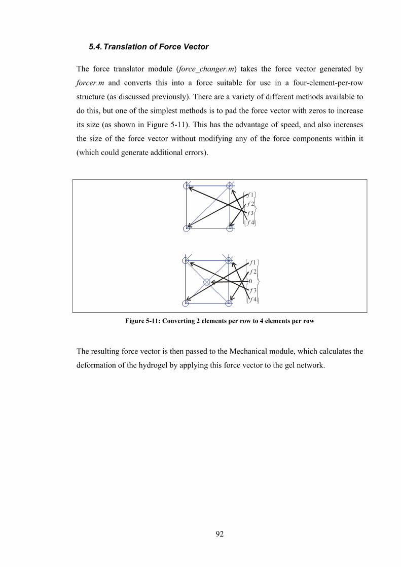
92

5.4. Translation of Force Vector

The force translator module (force_changer.m) takes the force vector generated by

forcer.m and converts this into a force suitable for use in a four-element-per-row

structure (as discussed previously). There are a variety of different methods available to

do this, but one of the simplest methods is to pad the force vector with zeros to increase

its size (as shown in Figure 5-11). This has the advantage of speed, and also increases

the size of the force vector without modifying any of the force components within it

(which could generate additional errors).

1234

ffff

⎧ ⎫⎪ ⎪⎪ ⎪⎨ ⎬⎪ ⎪⎪ ⎪⎩ ⎭

12

034

ff

ff

⎧ ⎫⎪ ⎪⎪ ⎪⎪ ⎪⎨ ⎬⎪ ⎪⎪ ⎪⎪ ⎪⎩ ⎭

Figure 5-11: Converting 2 elements per row to 4 elements per row

The resulting force vector is then passed to the Mechanical module, which calculates the

deformation of the hydrogel by applying this force vector to the gel network.

93

6. Mechanical Module

6.1. Introduction

The Mechanical module is the penultimate module in the overall model, and is used to

calculate the deformation of the hydrogel from the various forces calculated by the

previous modules. The Mechanical module receives information about the magnitude,

direction and location of forces being applied to the hydrogel. By using the theory of

linear elasticity, the module calculates the predicted deformation resulting from these

forces, which can then be displayed graphically. This provides a quick, easy method of

verifying the predictions of the overall model.

Figure 6-1: Position of Mechanical module in overall model

6.2. Assumptions

While a number of assumptions are made in the Mechanical module, possibly the most

significant are those related to the elasticity of the hydrogel. The Mechanical module

assumes that:

• The hydrogel material obeys linear elasticity relationships, and that the elasticity

of the gel is uniform and time invariant. Poly(acrylic acid) hydrogels are known

to consist of regions of high and low density [105], and this does cause spatial

variation in the hydrogel elasticity. Real hydrogels also possess viscoelastic

properties (and not purely elastic) which cause hysteresis effects. Some

hydrogels can also vary their elasticity under influence of an electric field [68],

further complicating material assumptions. In the case of this work however, the

assumption is justified by the fact that the hydrogel behaves linearly in

94

quasistatic situations and because the hydrogel is extremely elastic. The use of

this assumption drastically reduces the complexity of the equations that need to

be solved by the model.

• The gravitational and frictional forces experienced by the gel are negligible. The

gravity force is assumed to be countered by the upwards force on the lower

region of the hydrogel generated by the gel support. Friction may be assumed to

be negligible as the solvent surrounding the hydrogel acts as a lubricant, by

reducing the surface-to-surface contact (section 6.3.4) (as shown in Figure 6-2).

Although, these two forces are ignored in this model, the modular approach

followed throughout this work ensures that they could be readily added if

required.

Electrodes

Gravity force

Reaction

Rigid base

Solvent

Friction (negligible)

Figure 6-2: Gravitational and frictional forces


The Mechanical module takes as its input a force vector and returns a nodal

displacement vector as output. Hence, it is necessary to derive a governing equation to

describe the motion of an elastic body under the influence of an external force (Figure

6-3).

95

1 2

3

[M] x

y

Figure 6-3: Forces applied to a finite element

Newton’s second law (at time t) is ideally suited to this problem, and can be written as:

[ ]ttF M d=∑ (6.1)

where F is an externally-applied force, [M] is a mass matrix and d is a nodal

displacement vector. If elastic restoring and viscous damping forces (that act against the

externally-applied force) are considered, equation (6.1) can be rewritten as:

( ) [ ] [ ] [ ]t tt tF K d C d M d− − = (6.2)

where [K] is a stiffness matrix and [C] is a damping matrix. Equation (6.2) can then be

rearranged to give:

[ ] [ ] [ ]t t t tM d C d K d F+ + = (6.3)

In order to formulate the finite element approximation for equation (6.3), the mass,

stiffness and damping matrices must be calculated for each element and then assembled

into global mass, stiffness and damping matrices. For convenience, these matrices are

assumed to be independent of time, but could be readily modified to include time-

dependence if required.

6.3.1. Element Stiffness Matrix [K]

In order to calculate the element stiffness matrix, it is useful to simplify equation (6.3)

by assuming a purely elastic body with [M] = [C] = 0 (no inertia or damping). By

96

conservation of energy, the internal strain energy (elastic restoring energy) generated by

the body must then be equivalent to the external work applied (applied force). Thus,

under the influence of an externally applied force, an elastic body would deform and

cause strain energy in the amount [99]:

12

tstrainU dσ ε

Ω

= Ω∫ (6.4)

where σ is the stress and ε is the strain, integrated over the entire element area (Ω).

Equation (6.4) can also be written in the more familiar form:

12

EstrainU K d

Ω

⎡ ⎤= Ω⎣ ⎦∫ (6.5)

where [KE] is the element stiffness matrix.

From the fundamental definitions of elasticity, the engineering strain is defined in terms

of displacements by the equation:

0i

LL

ε ∆= (6.6)

where the change in length ∆L, is taken in the ith direction and L0 is the initial

longitudinal length of the element.

From equation (6.6), for a given displacement of u and v in the x- and y-directions

respectively, the two-dimensional strain vector can be written as [123]:

x

y

xy

uxvy

u vy x

εεγ

⎧ ⎫∂⎪ ⎪

∂⎪ ⎪⎧ ⎫⎪ ⎪∂⎪ ⎪ =⎨ ⎬ ⎨ ⎬∂⎪ ⎪ ⎪ ⎪

⎩ ⎭ ⎪ ⎪∂ ∂+⎪ ⎪∂ ∂⎩ ⎭

(6.7)

97

where εx, εy are the strain in the x- and y-directions respectively and γxy is the shear

strain.

In order to evaluate equation (6.7) in a finite element formulation, the shape functions

introduced in chapter 2 must be used. In this work, the element domain is discretised

using linear triangular elements with shape functions (H1, H2 and H3):

( ) ( ) ( )

( ) ( ) ( )

( ) ( ) ( )

1 2 3 3 2 2 3 3 2

2 3 1 1 3 3 1 1 3

3 1 2 2 1 1 2 2 1

121

21

2




= − + − + −⎡ ⎤⎣ ⎦

= − + − + −⎡ ⎤⎣ ⎦

= − + − + −⎡ ⎤⎣ ⎦

(6.8)

where the coordinates (xi , yi) are associated with the ith node (as shown in Figure 6-4).

(x1,y1) (x2,y2)

(x3,y3)

Figure 6-4: Finite element with local node numbers

By definition, any x- or y-displacement can be written in terms of the shape functions

and so a displacement of u and v (in the x- and y-directions, respectively) can be written

as: 3

13

1

( , ) ( , )

( , ) ( , )

i ii

i ii

u x y H x y u

v x y H x y v

=

=

=

=

∑

∑ (6.9)

98

which in matrix form becomes:

( )( )

1

1

1 2 3 2

1 2 3 2

3

3

0 0 0,0 0 0,

uv

H H H uu x yH H H vv x y

uv

⎡ ⎤⎢ ⎥⎢ ⎥⎢ ⎥⎧ ⎫ ⎡ ⎤

=⎨ ⎬ ⎢ ⎥⎢ ⎥⎣ ⎦⎩ ⎭ ⎢ ⎥

⎢ ⎥⎢ ⎥⎣ ⎦

(6.10)

Using equation (6.10) in equation (6.7) leads to:

131 2

1

231 2

2

33 31 1 2 2

3

0 0 0

0 0 0x

y

xy

uHH Huvx x xxuHH Hvvy y y yuu v H HH H H H

y x y x y x y x v

εεγ

⎧ ⎫⎡ ⎤⎧ ⎫ ∂∂ ∂∂ ⎪ ⎪⎢ ⎥⎪ ⎪∂ ∂ ∂∂ ⎪ ⎪⎢ ⎥⎪ ⎪⎧ ⎫

⎪ ⎪⎢ ⎥∂⎪ ⎪ ∂ ∂∂⎪ ⎪ = =⎨ ⎬ ⎨ ⎬ ⎨ ⎬⎢ ⎥∂ ∂ ∂ ∂⎪ ⎪ ⎪ ⎪ ⎪ ⎪⎢ ⎥⎩ ⎭ ⎪ ⎪ ⎪ ⎪⎢ ⎥∂ ∂ ∂ ∂∂ ∂ ∂ ∂

+⎪ ⎪ ⎪ ⎪⎢ ⎥∂ ∂ ∂ ∂ ∂ ∂ ∂ ∂⎩ ⎭ ⎣ ⎦ ⎩ ⎭

(6.11)

which in abbreviated form can be written as:

[ ] uε = B (6.12)

where [B] is known as the kinematic matrix. Substituting equation (6.8) into equation

(6.11) allows the [B] matrix to be written as:

[ ]( ) ( ) ( )

( ) ( ) ( )( ) ( ) ( ) ( ) ( ) ( )

2 3 3 1 1 2

3 2 1 3 2 1

3 2 2 3 1 3 3 1 2 1 1 2

0 0 01 0 0 0

2

y y y y y yx x x x x x

Ax x y y x x y y x x y y

⎡ ⎤− − −⎢ ⎥= − − −⎢ ⎥⎢ ⎥− − − − − −⎣ ⎦

B

(6.13)

99

For a triangle with three nodes having coordinates (x1,y1), (x2,y2) and (x3,y3), the area

(A) is given by the determinant [100]:

1 1

2 2

3 3

2 3 1 2 3 1 2 1 1 3 3 2

11 12

1

2

x yA x y

x yx y x y x y x y x y x y

=

+ + − − −=

(6.14)

In an isotropic material with plane stress, the strains in equation (6.7) are related to their

respective 2-dimensional stresses through Hook’s law [100]:

( )21x x yEσ ε νεν

= +−

(6.15)

( )21y y xEσ ε νεν

= +−

(6.16)

( )12 1xy xy

Eτ γν

=−

(6.17)

In a matrix form, equations (6.15)-(6.17) can be written as:

2

1 01 0

110 0

2

x x

y y

xy xy

Eσ ν εσ ν ε

ντ ν γ

⎡ ⎤⎢ ⎥⎧ ⎫ ⎧ ⎫⎢ ⎥⎪ ⎪ ⎪ ⎪=⎨ ⎬ ⎨ ⎬⎢ ⎥−⎪ ⎪ ⎪ ⎪⎢ ⎥−⎩ ⎭ ⎩ ⎭⎢ ⎥⎣ ⎦

(6.18)

or,

[ ] σ ε= D (6.19)

where D is a material properties matrix.

100

If the material has residual strains and stresses resulting from initial processing

conditions, then equation (6.18) can be extended to [117]:

[ ] ( ) 0 0σ ε ε σ= − +D (6.20)

where ε0 and σ0 are the residual strain and stress in the material. In this work, because

the polymer hydrogel is a highly elastic material at equilibrium under naturally small

loads, the residual stresses/strains are considered to be minimal and so are disregarded.

Using equations (6.12) and (6.19), the element stiffness matrix from equation (6.5) can

be written as:

[ ] ( )

[ ][ ]( ) [ ] [ ] [ ][ ]

tE

T

T

T

K

u

u

σ ε

ε ε

⎡ ⎤ =⎣ ⎦

=

=

=

D

D B B

B D B

(6.21)

since [D] is a symmetric matrix.

6.3.2. Element Mass Matrix [M]

The mass matrix provides the inertial term in equation (6.3), with its exact form

depending on the shape functions of the elements used. The general form of the mass

matrix for each element is given by:

[ ] [ ]e

TEM N N dρΩ

⎡ ⎤ = Ω⎣ ⎦ ∫ (6.22)

where ρ is the mass density and [N] is a matrix of shape functions integrated over the

entire element area (Ωe). Using the shape function matrix, equation (6.22) can be

written as:

101

[ ] [ ]

1 2 3 1 2 3

1 2 3 1 2 3

21 1 2 1 3

21 1 2 1 3

21 2 2 2 3

21 2 2 2 3

21 3 2 3 3

21 3 2 3 3

0 0 0 0 0 00 0 0 0 0 0

0 0 00 0 0

0 0 00 0 0

0 0 00 0 0

e

e

e

TE

T

M N N d

H H H H H Hd

H H H H H H

H H H H HH H H H H

H H H H Hd

H H H H HH H H H H

H H H H H

ρ

ρ

ρ

Ω

Ω

Ω

⎡ ⎤ = Ω⎣ ⎦

⎡ ⎤ ⎡ ⎤= Ω⎢ ⎥ ⎢ ⎥

⎣ ⎦ ⎣ ⎦

⎡ ⎤⎢ ⎥⎢ ⎥⎢ ⎥

= Ω⎢ ⎥⎢ ⎥⎢ ⎥⎢ ⎥⎢ ⎥⎣ ⎦

∫

∫

∫

(6.23)

which can be solved using the area integral identity [117]:

( )1 2 3! ! ! 2

!e

a b c ea b cH H H dAa b c

Ω

⋅ ⋅ ⋅ = Ω+ +∫ (6.24)

where Ωe is the area of the element. Using (6.24) in (6.23) gives:

2 0 1 0 1 00 2 0 1 0 11 0 2 0 1 00 1 0 2 0 1121 0 1 0 2 00 1 0 1 0 2

E AM ρ

⎡ ⎤⎢ ⎥⎢ ⎥⎢ ⎥

⎡ ⎤ = ⎢ ⎥⎣ ⎦⎢ ⎥⎢ ⎥⎢ ⎥⎣ ⎦

(6.25)

which is known as the consistent mass matrix. The thickness of the element is assumed

to be unity and is not shown in equation (6.25). In order to simplify equation (6.25), the

mass is sometimes assumed to be “lumped” at the nodes in equal parts.

For triangular elements (with three nodes per element) the mass matrix then becomes:

[ ]63E AM Iρ⎡ ⎤ =⎣ ⎦ (6.26)

102

where [I6] is a 6×6 identity matrix. In practice, equation (6.25) and (6.26) give similar

results, but the use of equation (6.26) can be computationally advantageous since it can

be stored in less memory, as will be discussed in section 6.4.

6.3.3. Element Damping Matrix [C]

The form of the damping matrix is almost identical to the mass matrix, and also depends

on the specific shape functions used. In general terms, the damping matrix for each

element is given by:

[ ] [ ]e

TEC N N dµΩ

⎡ ⎤ = Ω⎣ ⎦ ∫ (6.27)

where µ is a matrix of viscosity parameters and [N] is a matrix of shape functions

integrated over the entire element area (Ωe).

In reality, exact knowledge of the viscosity parameters is often difficult and so the

damping matrix is sometimes approximated as [117]:

E E E

R RC M Kα β⎡ ⎤ ⎡ ⎤ ⎡ ⎤= +⎣ ⎦ ⎣ ⎦ ⎣ ⎦ (6.28)

where αR and βR are experimentally determined parameters and [M] and [K] are the

mass and stiffness matrices from equations (6.21) and (6.22). Equation (6.28) is known

as the Raleigh damping, and has some computational advantages over equation (6.27).

By adjusting the αR and βR constants, different system effects can be achieved. For

example, by biasing β with respect to α, high frequency over-damping can be achieved

that helps counter any high frequencies generated by using the finite element

approximation.

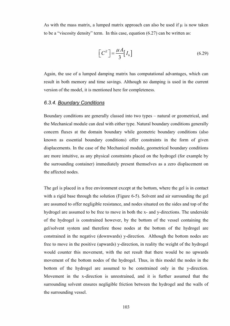
103

As with the mass matrix, a lumped matrix approach can also be used if µ is now taken

to be a “viscosity density” term. In this case, equation (6.27) can be written as:

[ ]63E AC Iµ⎡ ⎤ =⎣ ⎦ (6.29)

Again, the use of a lumped damping matrix has computational advantages, which can

result in both memory and time savings. Although no damping is used in the current

version of the model, it is mentioned here for completeness.

6.3.4. Boundary Conditions

Boundary conditions are generally classed into two types – natural or geometrical, and

the Mechanical module can deal with either type. Natural boundary conditions generally

concern fluxes at the domain boundary while geometric boundary conditions (also

known as essential boundary conditions) offer constraints in the form of given

displacements. In the case of the Mechanical module, geometrical boundary conditions

are more intuitive, as any physical constraints placed on the hydrogel (for example by

the surrounding container) immediately present themselves as a zero displacement on

the affected nodes.

The gel is placed in a free environment except at the bottom, where the gel is in contact

with a rigid base through the solution (Figure 6-5). Solvent and air surrounding the gel

are assumed to offer negligible resistance, and nodes situated on the sides and top of the

hydrogel are assumed to be free to move in both the x- and y-directions. The underside

of the hydrogel is constrained however, by the bottom of the vessel containing the

gel/solvent system and therefore those nodes at the bottom of the hydrogel are

constrained in the negative (downwards) y-direction. Although the bottom nodes are

free to move in the positive (upwards) y-direction, in reality the weight of the hydrogel

would counter this movement, with the net result that there would be no upwards

movement of the bottom nodes of the hydrogel. Thus, in this model the nodes in the

bottom of the hydrogel are assumed to be constrained only in the y-direction.

Movement in the x-direction is unrestrained, and it is further assumed that the

surrounding solvent ensures negligible friction between the hydrogel and the walls of

the surrounding vessel.

104

OOOOOOOOO

OOOOOOOOO

OOOOOOOOO

OOOOOOOOO

OOOOOOOOO

OOOOOOOOO

OOOOOOOOO

OOOOOOOOO

OOOOOOOOO

OOOOOOOOO

OOOOOOOOO

OOOOOOOOO

OOOOOOOOO

OOOOOOOOO

Gel

Solvent

BaseNode free to move in xNo movement in y

Node free to move in x and y

Figure 6-5: Constrained nodes in hydrogel

6.3.5. Velocity and Displacement Through Time Integration

In order to calculate the nodal displacements at each timestep, the Mechanical module

employs a central-difference time integration (CDTI) scheme to solve equation (6.3).

While a wide variety of time integration schemes are available, the CDTI scheme is

frequently used in structural mechanics problems since it can provide displacment,

velocity and acceleration data for the system. The CDTI is only conditionally stable

however, and so care must be taken to ensure an appropriate timestep is selected. In this

work, the CDTI is implemented in the “summed” form [124], which provides

displacement, velocity and acceleration data for each node in the system for each

timestep. While the Mechanical module only utilises displacement data, the availability

of velocity and acceleration data ensures that it could be used in later modules if

required.

The CDTI immediately presents two potential problems, and these must be examined

before the suitability of the scheme can be evaluated for use in the Mechanical module.

The first problem is that it requires an initial velocity solution at the fictitious time of

-0.5∆t (Figure 6-6). This can be calculated by using the standard time integral

approximation:

00.5

tt d d

dt

−∆− ∆ −

=∆

(6.30)

where 0d is the initial displacement and td −∆ is the displacement at the fictitious

time -∆t.

105

time d 0

∆t ∆t ∆t

d -∆t d + ∆t

d -0.5∆t.

Figure 6-6: Calculating fictitious displacements and velocities

The fictitious displacement at time -∆t can be calculated using the linear relationships

between displacement, velocity and acceleration:

20 00

2t t td d t d d−∆ ∆

= − ∆ + (6.31)

where 0d and 0

d are the velocity and acceleration at t = 0. If the initial

displacement, velocity and acceleration are all zero, then equation (6.31) can be

simplified to:

0t td d−∆ = (6.32)

Using equation (6.32) in equation (6.30) gives an initial velocity at t = -0.5∆t of zero.

Therefore, the need for a fictitious initial velocity does not preclude the use of the CDTI

scheme in this model.

The second potential problem with the CDTI scheme is that displacements and

accelerations are calculated at the same timestep, but velocities are calculated midway

through each timestep (i.e. at t + 0.5∆t). This is only problematic if velocities are

required for each timestep, whereas this model only utilises the nodal displacements.

Thus, the misalignment of the velocity data does not preclude the use of the CDTI

scheme in this work.

During each timestep, the Mechanical module first calculates the acceleration by

rearranging equation (6.3) to give:

( )1[ ] [ ] [ ]t tt td M F C d K d−= − − (6.33)

106

where the initial displacements and velocities of each node are assumed to be zero. In

order to calculate the velocity at a time t + 0.5∆t, the model utilises the relationship

between acceleration and velocity:

0.50.5

0.5

t tt t

t t

d d dt+ ∆

+ ∆

− ∆

= ∫ (6.34)

which in discrete form can be expressed as:

0.5 0.5t t t t td d t d

+ ∆ − ∆= + ∆ (6.35)

Finally, to calculate the displacement at a time t + ∆t, the model again uses the

relationship between velocity and displacement:

t t

t t

t

d d dt+∆

+∆ = ∫ (6.36)

which in discrete form can be expressed as:

0.5t tt t td d t d+ ∆+∆ = + ∆ (6.37)


The Mechanical module (mech.m) is called during each time iteration, and uses

information on the magnitude and location of the nodal forces from the Force module,

as well as the nodal displacement and velocity information from the previous timestep.

A complete listing of the Mechanical module and the different scripts is given in

Appendix B.

107

As input, the Mechanical module is passed the following information:

• Mechanical properties such as Young’s modulus, Poisson’s ratio, mass density

and viscous damping coefficient. The mechanical properties are determined

experimentally and from values in literature (eg [125]). These constants could

also have been stored within the Mechanical module, but for ease of use are all

accumulated in the main control program.

• Geometrical parameters on the hydrogel such as global coordinates and nodal

elements. The number of nodal degrees-of-freedom (two, for x- and y-

displacement) is included in the Mechanical module, as it is the only module

with nodes possessing more than one degree-of-freedom.

As with previous modules, the Mechanical module is run in a number of steps.

Step 1

The Mechanical module first initialises the global stiffness ([K]), mass ([M]) and

damping ([C]) matrices along with their associated matrices. By definition, these

matrices are also square matrices of size 2n×2n elements, where n is the number of

nodes in the system, each with two degrees-of-freedom. The initialisation of these

matrices is performed locally in the Mechanical module and not passed from the main

control program, as the passing of large matrices is both time and memory intensive.

The module also sets up the boundary conditions, which for this work are of a

geometrical type.

Step 2

Once the global matrices are initialised, the module calculates the material properties

matrix [D] from the passed Mechanical parameters (for example, the Young’s

modulus). To calculate the material properties matrix [D], the script fematiso.m is called

which implements equation (6.18).

Step 3

The matrix then iteratively calculates the element matrices for each element in the

hydrogel. The module first calculates the system degree-of-freedom for each of the

three nodes associated with each element. The Mechanical module then proceeds to

calculate the area of that element, which is required by the stiffness matrix.

108

Step 4

Once the module has calculated the area of each element, the kinematic matrix [B] and

stiffness matrix [K] for each element is calculated. To calculate the kinematic matrix

[B] in equation (6.13), the module first calculates the area of the triangular element

using equation (6.14). Using the shape functions from equation (6.11), the module

calculates the x- and y-displacements using equation (6.8). The kinematic matrix [B]

for each element is then assembled using the script fekine2d.m. To compute the element

stiffness matrix [KE] for each element, the module uses equation (6.21).

The scripts used to generate the [B] and [D] matrices were written by Kwon and Bang

[99] and are used in their original forms as discussed previously.

Step 5

The module then calculates the damping matrix [C] for each element, but as discussed

earlier, this is not used in this work.

Step 6

Finally, the Mechanical module calculates the mass matrix [M] for each element in the

hydrogel. To calculate the mass [M]E and damping [C]E matrices for each element, the

Mechanical module calls the script mmtriang.m, which can calculate consistent or

lumped matrices depending on the argument passed to it. The similarity between the

form of the mass and damping matrices allows mmtriang.m to be used for both, with a

different constant (mass density or viscosity) being passed for each matrix.

Step 7

The module then repeats steps 3-6 to assemble the stiffness, damping and mass matrices

for each element into a global stiffness, damping and mass matrix. The script

feasmbl1.m is used, which places the element matrices into the correct location within

the global matrix.

Step 8

Once the stiffness, damping and mass matrices are known for the system, the module

proceeds to perform time integration in order to calculate the displacement. The module

first calculates the acceleration for each node in the system for the current timestep

using equation (6.33). As discussed in previous chapters, the inversion of the mass

109

matrix can also be accomplished by using the MATLAB ldivide (left divide) command

subject to the mass matrix meeting certain requirements [118].

Step 9

Once the acceleration is known, the Mechanical module applies the boundary conditions

discussed in the first step to calculate the velocity for each node for the following

timestep. To apply the boundary conditions, mech.m initialises a vector containing the

degrees-of-freedom associated with the nodes along the bottom of the hydrogel. As

discussed in section 6.3.4, these nodes are constrained in the y-direction, but free to

move in the x-direction.

Step 10

Using this velocity, the module uses equation (6.37) to calculate the displacement of

each node in the hydrogel for the following timestep. Using this method, the

deformation of each node in the hydrogel can be calculated. To calculate the velocity

and displacement vectors for the t+1 timestep, the Mechanical module uses equations

(6.35) and (6.37).

The module then returns these velocities and displacements to the main control

program, where they are used to generate deformation plots. The greatest concern in this

module is the memory allocation problems associated with MATLAB. By default,

MATLAB defines all matrix elements as type double, each of which take 8 bytes of

memory. Thus, for a moderate size finite element model with 1,000,000 nodes there are

2,000,000 degrees-of-freedom. The element matrices are then each (2,000,000)2 =

2×1012 elements in size and each matrix is therefore 32Tb (32×1012bytes) large. This is

unmanageable for a standard desktop computer, and methods need to be sought to

enable MATLAB to deal with large matrices more efficiently. While MATLAB does

offer the ability to create 8-, 16- and 32-bit signed and unsigned integers, it only permits

the use of double values in mathematical calculations [126] and so single integer types

still need to be converted in order to be used.

The situation can be improved by realising that although the stiffness, mass and

damping matrices are large, they are also sparse and therefore can be dealt with in

MATLAB using the sparse matrix types. This is similar to the approach used by

commercial FEA programs. In MATLAB, sparse matrices are still strored in double-

precision format, but this effectively squeezes the zero elements from the matrix which

110

dramatically reduces its size. While this situation is not ideal, in practice it has not

produced any significant errors in the results. A flowchart of the Mechanical module is

shown in Figure 6-7.

Set up GLOBAL stiffness, mass and damping

matrices

Constants from MAIN

Set up boundary conditions matrix

Calculate [D] matrix

For i=1 to number of elements

Extract nodes and DOF associated

with element

Calculate area and derivative of

element

Compute [B] matrix

Compute element stiffness matrix [K]

Compute mass matrix [M]

Assemble [K],[M] and [C] matrices

into GLOBAL matrices

All elements processed

Calculate acceleration for

current time

Apply boundary conditions

Calculate velocity for next timestep

Calculate displacement for

next timestep

NO YES

Return to MAIN

Figure 6-7: Flowchart of Mechanical module

111

7. Optical Module

7.1. Introduction

Whether the gel is used for optical applications or an actuator, the output of the

Mechanical module can be used without affecting the generality of the whole model. In

this work however, the Optical module is the final component in the overall model, and

as such returns the final result of the model (i.e. a change in focal length). It takes as its

input the deformation calculated by the Mechanical module and uses this to calculate

the theoretical change in the radius of curvature and refractive power (Figure 7-1).

Figure 7-1: Position of Optical module in overall model

The Optical module is not a critical part of the model, as its output is not required by

any other modules in order to function (e.g. the Mechanical or Chemical modules). For

this reason, the Optical module is also one of the smallest modules in the model.

7.2. Assumptions

As with all the modules in this work, the Optical module makes some general

assumptions (discussed earlier) and also some assumptions related only to this chapter.

Some of the assumptions that are particularly relevant to this chapter are:

1. The module assumes that the deformation of the upper hydrogel lens surface can

be approximated as either a spherical or paraboloidal surface. Since the

deformation is taken to be symmetrical about the y-axis, and both a sphere and a

paraboloid are symmetrical functions about the y-axis, this assumption is

reasonable. This approximation has also been used by other authors, for example

Sugiura [97] who developed an analytical formulation for a variable focal length

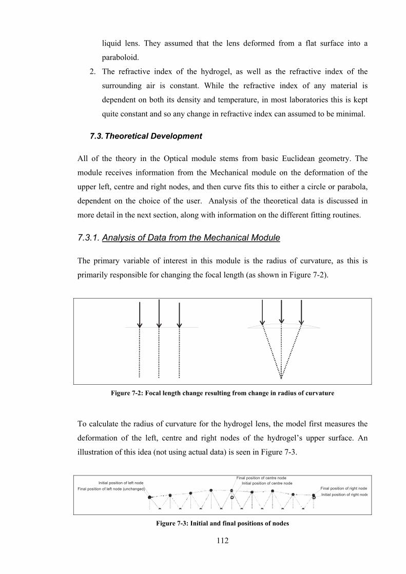
112

liquid lens. They assumed that the lens deformed from a flat surface into a

paraboloid.

2. The refractive index of the hydrogel, as well as the refractive index of the

surrounding air is constant. While the refractive index of any material is

dependent on both its density and temperature, in most laboratories this is kept

quite constant and so any change in refractive index can assumed to be minimal.


All of the theory in the Optical module stems from basic Euclidean geometry. The

module receives information from the Mechanical module on the deformation of the

upper left, centre and right nodes, and then curve fits this to either a circle or parabola,

dependent on the choice of the user. Analysis of the theoretical data is discussed in

more detail in the next section, along with information on the different fitting routines.

7.3.1. Analysis of Data from the Mechanical Module

The primary variable of interest in this module is the radius of curvature, as this is

primarily responsible for changing the focal length (as shown in Figure 7-2).

Figure 7-2: Focal length change resulting from change in radius of curvature

To calculate the radius of curvature for the hydrogel lens, the model first measures the

deformation of the left, centre and right nodes of the hydrogel’s upper surface. An

illustration of this idea (not using actual data) is seen in Figure 7-3.

Initial position of left nodeFinal position of left node (unchanged) Final position of right node

Initial position of right node

Final position of centre nodeInitial position of centre node

Figure 7-3: Initial and final positions of nodes

113

By comparing the height of the centre node with the heights of the nodes at the edge of

the surface, the Optical module calculates the average change in height, ∆y as shown in

Figure 7-4.

∆y

Figure 7-4: Curve fitting hydrogel deformation

In general, maximum deformation occurs at the centre of the top hydrogel surface while

the top edges experience minimal deformation. The model first verifies this assumption,

and returns an error message if this criterion is not met. The model then uses this change

in height with the radius of the lens to fit the deformation to either a sphere or a

parabola and calculate the new focal length (assumed initially to be infinity). A

comparison of the circular and parabolic line fits is shown in Figure 7-5, with each

fitting routine discussed in more detail in the following sections.

Figure 7-5: Comparison of sphere and parabolic line fit (adapted from [127])

7.3.2. Curve Fitting to a Parabola

From basic geometry, the equation for a parabola in Cartesian coordinates is given by

the equation:

2 4x fy= (7.1)

114

where f is the distance from the vertex (assumed to be at the origin) to the focus of the

parabola. By examining Figure 7-4 and Figure 7-6, it can be seen that the difference in

height between the left and right nodes with the centre node is given by the distance ∆y.

Thus, equation (7.1) can be solved for the focal length f by noting that y = ∆y at x = r,

where r is the radius of the hydrogel disc. To ensure a best fit, the Optical module uses

the average distance between the left/centre and right/centre nodes, which generally

results in one of the edge nodes lying below the fitted line, and the other edge node

lying above the fitted line.

Figure 7-6: Curve fitting to a parabola

7.3.3. Curve Fitting to a Circle

The Optical module can also fit the theoretical deformation to a circle, although this

generally results in a worse fit than for a parabola. To calculate the focal length for data

which has been fitted to a circle, slightly more calculations are required than for a

parabola. Using circle geometry, the following relationships can be noted (Figure 7-7):

( )

2 22

4 2

c R d

h R h

= −

= − (7.2)

which can be rearranged to give:

2 24

8c hR

h+

= (7.3)

115

R

c

s

θ

h

d

Figure 7-7: Curve fitting to a circular surface

Equation (7.3) contains three unknowns – R, c and h. Clearly, from Figure 7-4 it can be

seen that h represented the change in height (∆y) and c is the radius of the lens. This

allows equation (7.3) to be solved for the radius of curvature, R. The focal length, f is

then given by half of the radius of curvature:

2Rf = (7.4)

7.3.4. Relating the Curvature to the Refractive Power

Once the radius of curvature is known together with the refractive indices of the

hydrogel and air, the Optical module can also calculate the refractive power of the

resulting lens using [128]:

n nPR

′−= (7.5)

where n is the refractive index of the medium the ray passes through before reaching the

surface and n’ is the refractive index of the medium on the emergent surface. For the

first refracting surface, n=n1 and n’=n2 while for the second refracting surface n=n2 and

n’=n1.


Initially the Optical module is passed information on the overall size of the hydrogel

region; the initial positions of all nodes in the hydrogel, the deformation of each node in

the hydrogel region, the width of the hydrogel region (in meters) and the size of each

116

element in the hydrogel (in meters). As with previous modules, the Optical module is

implemented in a number of steps. A complete listing of the Optical module and the

different scripts is given in Appendix B.

Step 1

The Optical model first uses the variables gel_flg_node and col to determine the centre

node of the hydrogel region, as well as the two nodes on the edges of the top of the

hydrogel region.

Step 2

Using the information obtained from step 1, the Optical module calculates the change in

position of the centre node, as well as the change in position of the two side nodes

(Figure 7-3). The module can then calculate the resulting change in height, ∆y.

Step 3

The model asserts that the deformation of the side nodes is minimal compared to the

deformation of the centre node, and returns an error if this is found to be false.

Step 4

Using the width of the hydrogel and average change in height, the Optical module then

fits the deformation to either a parabola or a circle, depending on the choice of the user.

Once fitted, the module returns the focal length and theoretical refractive power of the

hydrogel lens to the user. A flowchart of the Optical module is shown in Figure 7-8.

117

Identify left, centre and right nodes on

top surface of hydrogel

Constants from MAIN

Return to MAIN

Measure change in height of

CENTRE node

Measure change in height of RIGHT

node

Measure change in height of LEFT

node

Calculate average change in height,

y

Deformation of edge nodes small?

Error code returned

Fit to sphere or parabola?

Calculate focal length and

refractive power

Calculate focal length and

refractive power

NO

YES

SPHEREPARABOLA

Figure 7-8: Flowchart of Optical module

∆

118

8. Experimental Validation

8.1. Introduction

In order to verify the theoretical predictions made by the model, experiments were

conducted on a number of gel samples. The preparation and measuring methods utilised

in these experiments are discussed in this chapter.

8.2. Preparation of Hydrogels

To prepare the polymer hydrogels used in this work, an acrylic acid (AAC) monomer is

polymerised using thermally-triggered free radical polymerisation. The method of

polymerisation was developed by the author [30] and is based on a combination of

methods developed by others [105, 129-132].

First, 4.8mL (70mmol) of AAC (Alfa Aesar, 99%, used as received), and dissolved into

50mL of doubly-distilled deionised water (DI) to create a 1.277 mol L-1 solution. In an

aqueous solution, the carbolic acid part of the AAC monomer (COOH) dissociates

according to the chemical equation:

[ ]COOH H COO+ −⎡ ⎤ ⎡ ⎤⎣ ⎦ ⎣ ⎦ (8.1)

where the amount of dissociation is represented by the acid dissociation constant (Ka):

[ ]( )a

H COOK COOH

COOH

+ −⎡ ⎤ ⎡ ⎤⎣ ⎦ ⎣ ⎦ = (8.2)

Using a Ka value of 5.74×10-5 [133], the concentration of [H+] and [COO-] ions for a

1.277 mol L-1 pre-gel solution can be found. This provides an initial [COO-]

concentration of 8.48×10-3 mol L-1 and a theoretical pH of 2.07. The commercial AAC

was inhibited with 200ppm 4-methoxyphenol (MEHQ), which when combined with

oxygen (air) prevents runaway polymerisations. Although the MEHQ can be removed

from the AAC, Cutié et al. [134] found that in isothermal persulfate-initiated

119

polymerisations, MEHQ acted as an inhibitor and slowed, but did not prevent a

polymerisation from occurring.

In order to increase the swelling capacity of the poly(acrylic acid) (PAAC) hydrogel, the

monomer solutions were pre-neutralised using 5.6mL (28mmol) of 5 mol L-1 NaOH

(Univar, analytical grade). To describe the effects of altering polymerization conditions,

Elliot et al. [135] developed a kinetic model and used it to show that by increasing the

amount of water present during polymerization, the amount of swelling that can be

achieved is increased. This was explained as an increase in cyclization, whereby the

polymer chain essentially links up with itself. Elliot also showed that performing the

polymerisation in a basic environment causes the cyclization to decrease, since the

carboxylic groups become ionized and move further apart (due to electrostatic

interactions). For this reason, polymers formed under acidic conditions swelled to only

1/3 of the volume of those prepared under basic conditions. Silberberg-Bouhnik et al.

[2] performed similar experiments and showed that maximum swelling can be achieved

using an approximately 35% neutralised PAAC gel. In this work however, a 40%

neutralised gel is used for convenience. One disadvantage of using pre-neutralised AAC

however, is that the polymerisation rate is known to decrease with increasing pH [136].

This effect can be counteracted by neutralising the PAAC hydrogel after

polymerisation, but Yin et al. [137] has suggested that this may generate different

polymer structures to those created using pre-neutralised AAC.

The effect of the addition of NaOH to the pre-gel solution can be described by the

chemical equation:

[ ] [ ]2[ ]COOH OH H O COO− −⎡ ⎤+ ⎣ ⎦ (8.3)

where the spectator Na+ ions in equation (8.3) have been omitted for clarity. The

addition of 28mmol of NaOH neutralises an equivalent number of moles of AAC,

leaving 42mmol of AAC. The new concentrations of AAC and NaOH are then given

by:

120

[ ]20

1

20

1

42

4260.4

0.6953

28

2860.4

0.46358

AAC NaOH H

AAC NaOH H

mmolCOOHVOL VOL VOL

mmolml

molL

mmolCOOVOL VOL VOL

mmolml

molL

−

−

−

=+ +

=

=

⎡ ⎤ =⎣ ⎦ + +

=

=

(8.4)

where VOLi is the volume of component i. Using the concentrations calculated in

equation (8.4), the theoretical pH of the pre-gel solution can be calculated to be 4.06.

Equation (8.3) provides the concentration of COO- and Na+ ions in the pre-gel solution,

which are assumed to remain constant as the hydrogel polymerises. Equations (8.2) and

(8.3) can therefore be used to provide the initial concentrations of ions in the hydrogel

region

In order to create a hydrogel, the pre-gel solution must be mixed with a suitable

crosslinking agent that links the polymer chains together and provides structural

rigidity. Two of the most common thermally-initiated crosslinkers are N,N-methylene-

bis-acrylamide (BIS) and trimethylol-propanetriacrylate (TMPTA), and each provides

certain advantages and disadvantages. Yin et al. [137] studied the solubility of both BIS

and TMPTA in AAC, and found almost no difference when using unneutralised AAC,

but found that BIS was 50% more efficient than TMPTA when using partially

neutralised AAC.

The choice of crosslinker is also important in determining the optical properties of the

formed PAAC hydrogel. Travas-Sejdic et al. [138] showed that the use of hydrophobic

crosslinkers (such as BIS) creates static inhomogeneities within the polymer matrix, and

that the magnitude of these inhomogeneities is directly dependent on the amount of

crosslinker added. Pekcan et al. [105] extended on this work by showing that the

intensity of 440nm photons moving through the hydrogel decreased as crosslinker

concentration was increased. This effect was also confirmed by the author [34].

121

Thus, to preserve the optical properties of the formed PAAC hydrogel, it is necessary to

use the smallest amount of crosslinker possible. Given its increased solubility in

partially neutralised AAC, BIS is clearly a more suitable crosslinker for use in this work

and Applichem Ultrapure BIS is used as the crosslinking agent for all experiments. The

crosslinker concentration also affects the structural properties (eg elasticity) of the

hydrogel, and thus must be above some empirically determined minimum value. In this

work, it was found that a BIS concentration of 2% (by mole) of monomer provided

sufficient structural rigidity while not overly affecting the transparency of the formed

hydrogel.

The pre-gel solution consisting of AAC, NaOH and BIS crosslinker is then placed under

vacuum and stirred vigorously for 15 minutes to ensure all components are thoroughly

mixed. Some gel-preparation methods also bubble nitrogen gas through the pre-gel

solution to displace any free oxygen that may be present (and act as an inhibitor). This

technique was investigated for this work, but was found to have almost no effect on the

produced hydrogel, and so was not used.

After 15 minutes of stirring, the seal of the vacuum was broken and 0.04g potassium

persulfate (KPS) (Scientific Supplies, AR grade, used as supplied) and 10µL of

N,N,N’,N’-tetramethylethylenediamine (TEMED) (Sigma, electrophoresis grade, used

as supplied) were added to the pre-gel solution. KPS is a thermally-triggered

polymerisation initiator, and is used to provide free radicals to the pre-gel solution. The

use of TEMED is not essential for polymerisation to occur but it does act as an

accelerator, and given the slightly higher pH, is considered essential in this work. The

pre-gel solution was then again placed under vacuum and thoroughly stirred for a

further 5 minutes.

The solution was then transferred to one or more glass Petri dishes (depending on the

required heights of the PAAC hydrogels), with a diameter of 10cm and height of 1cm.

The Petri dishes were placed into a vacuum oven (Lab-line, DuoVac 3610) at a

temperature setting of 70oC and pressure of -44kPa until polymerisation was complete

(typically 1.5 hours). It was found experimentally that when the oven was set to

temperatures below 70oC, no polymerisation occurred and that when the oven was set to

temperatures above 80oC, the pre-gel solution evaporated (the lower boiling point

resulting from the decreased pressure). The use of a vacuum was also found to be

122

necessary, as performing the polymerisations in air tended to leave a rippled effect on

the surface of the formed hydrogels. For optical applications, these ripples are

unacceptable.

Once completely polymerised, the hydrogel discs were removed from the oven and

allowed to cool. When cooled, the discs were thoroughly washed using DI water and

allowed to equilibrate with the atmosphere for a period of 24 hours.

In order to conduct swelling experiments, smaller gel discs were cut from the Petri

dishes using a sharpened glass cylinder. The diameter of these discs was constrained by

the cylinder to be 19mm, while the height of the disc was controlled by the amount of

pre-gel solution used during preparation. These discs were then used without any further

modifications (Figure 8-1).

Figure 8-1: Pre-cut gel discs

8.3. Hydrogel Swelling Dynamics

In order to investigate the swelling dynamics of the polymer hydrogel discs, the discs

were placed into a NaCl solution and subjected to an external voltage of 5, 7.5 or 10V.

From previous work [30], it is known that the type/material/location of the electrodes

used in swelling experiments affects the deformation of the PAAC hydrogel and

information on the type and location of electrodes needed to generate the required

deformation are known a priori. Experiments were conducted using a ring anode

(diameter 60mm, height 3mm) and a thin disc-shaped cathode (diameter 15mm), as

shown in Figure 8-2. Both electrodes were made of high-purity electrical grade

aluminium (Ling In Electronics Company Ltd).

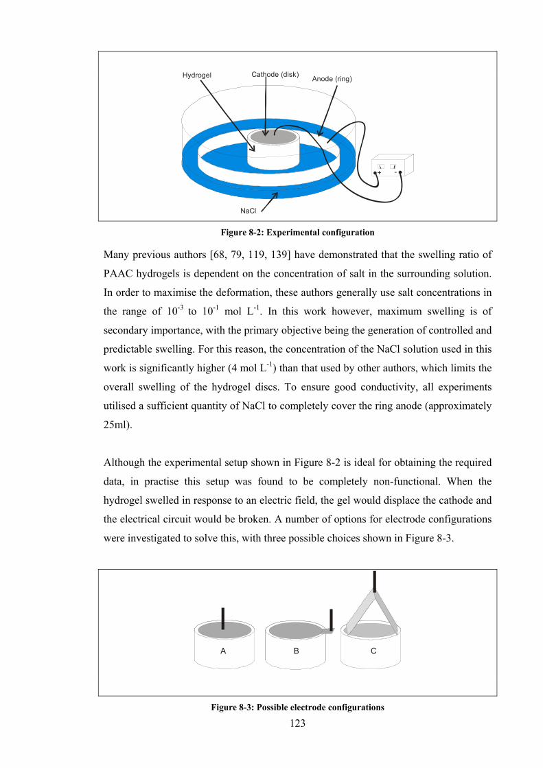
123

+ -

Cathode (disk) Anode (ring)

NaCl

Hydrogel

Figure 8-2: Experimental configuration

Many previous authors [68, 79, 119, 139] have demonstrated that the swelling ratio of

PAAC hydrogels is dependent on the concentration of salt in the surrounding solution.

In order to maximise the deformation, these authors generally use salt concentrations in

the range of 10-3 to 10-1 mol L-1. In this work however, maximum swelling is of

secondary importance, with the primary objective being the generation of controlled and

predictable swelling. For this reason, the concentration of the NaCl solution used in this

work is significantly higher (4 mol L-1) than that used by other authors, which limits the

overall swelling of the hydrogel discs. To ensure good conductivity, all experiments

utilised a sufficient quantity of NaCl to completely cover the ring anode (approximately

25ml).

Although the experimental setup shown in Figure 8-2 is ideal for obtaining the required

data, in practise this setup was found to be completely non-functional. When the

hydrogel swelled in response to an electric field, the gel would displace the cathode and

the electrical circuit would be broken. A number of options for electrode configurations

were investigated to solve this, with three possible choices shown in Figure 8-3.

A B C

Figure 8-3: Possible electrode configurations

124

Figure 8-3A involved placing an additional wire onto the cathode disc, but this was

found to restrain the swelling of the gel in the vertical direction. Figure 8-3B extended

on this idea by moving the wire to one side of the cathode. However, when the hydrogel

swelled, it pushed the cathode off to the side and resulted in a short circuit. Figure 8-3C

was a further improvement on Figure 8-3B based on a triangle, and was found to

function the best of all methods investigated. The vertical sides of the triangle provide

the rigidity necessary to hold the electrode in place, while the bottom side of the triangle

is able to deform in the vertical direction (and thus does not prevent the gel from

swelling, as in Figure 8-3A). The operation of the triangular cathode is shown in Figure

8-4.

Vertical sides provide rigidity

Bottom side free to deform

Figure 8-4: Triangular cathode

To record the deformation of the hydrogel cylinders during swelling, a digital video

camera (Sony TRV25E) was placed adjacent to the gel/solvent system (as shown in

Figure 8-5). Data was recorded at a resolution of 720×625, 25fps and then down-

converted into 640×480, 25fps Microsoft Windows Media format® (WMF) file to allow

for easier manipulation of the video data.

125

+ -

Power Supply

Cathode (disk)

Anode (ring)

Figure 8-5: Recording gel swelling data

Using a standard video editing program (TMPGEnc, Pegasys Inc), frames were

captured from the video file at 30s intervals and manually analysed. An example of a

captured frame is shown in Figure 8-6, along with an outline showing the positions of

the anode, cathode and gel. A complete series of captured images is shown in

Appendix A.

GELANODE

CATHODE

Figure 8-6: Captured frame

Although some image recognition software can automatically identify and measure the

gel deformation, in this case a number of factors could interfere with the measurement.

The transparent nature of the hydrogel makes focusing and boundary identification

difficult, and the liquid exuded from the hydrogel causes stray reflections which can

126

confuse imaging software. For this reason, data analysis is performed manually for each

frame, which should ensure consistent measurement errors, and also eliminates the two

aforementioned problems. To measure the deformation, the distances of three

strategically important points on the hydrogel are measured relative to the fixed anode

(as shown in Figure 8-7). This approach is similar to methods employed by Achilleous

et al. [72] and Marra et al. [140] who used a laser to etch a grid onto the gel samples

and then measured the deformation between points on the grid.

GEL

ANODE

CATHODE Height ofCentre Height

ofRight

Height ofLeft

Figure 8-7: Measuring gel dimensions

The deformation of the centre of the hydrogel is possibly the most important data set, as

this is where the maximum deformation is predicted to occur. Since each swelling

experiment utilises a new gel disc, it is difficult to achieve identical positioning and

lighting for each experiment. Therefore, to improve the comparability of different

experiments, the deformations of the gel edges were also measured. A readily

identifiable point on the gel edge is chosen, and then tracked as the hydrogel swells.

This also provides a method of observing the relative deformation of the hydrogel

relative to the centre. To account for any differences in camera positioning, the

measured deformations are scaled to ensure a similar scale for all experiments. This is

accomplished by using knowledge of the measured dimensions of the gel and

comparing this to the dimensional recorded on film.

8.4. Mechanical and Optical Properties

As well as providing validation for the overall model, many of the constants required by

the model are obtained through the use of experimental methods.

Mechanical parameters (such as Young’s modulus and Poisson’s ratio) are highly

variable for different polymer hydrogels, and depend on a number of intrinsic (such as

preparation conditions) and extrinsic properties (such as ambient temperature). Johnson

127

et al. [125] performed a variety of tests on pH-sensitive 2-hydroxyethyl methacrylate

(HEMA)-acrylic acid (AAC) gels to determine the relationships between ultimate

tensile strength, Young’s modulus and percentage elongation at break with changes in

pH, crosslinker weight percentage and polymerisation time. Johnson found that the

Young’s modulus for HEMA-AAC gels varied from 0.03MPa to 124MPa for

crosslinker weight percentages in the range 0.2-20 wt%. He also demonstrated that as

the hydrogel swells, its Young’s modulus decreased, and for this reason can only be

considered constant for small deformations. Johnson also measured the average

Poisson’s ratio for swollen and unswollen hydrogels, and obtained an average value of

0.43. Mahaffy et al. [141] used atomic force microscopy (AFM) to measure the

Young’s modulus and Poisson’s ratio for an AAC hydrogel with BIS content of 0.8

wt%. They obtained a value of 2160Pa for the Young’s modulus and 0.33 for the

Poisson ratio. Matsuda [142] and Miyakazi [143] performed experiments on

temperature-sensitive AAC copolymers, and obtained values in the order of 50MPa for

gels with crosslinker amounts of 0.3-10 mol%. There is also some evidence to suggest

that an externally-applied electric field alters the modulus of elasticity [55], which is

clearly of importance in this work. Experimental validation of this modulus change is

somewhat limited however, and was also not perfromed in this work. It is anticipated

future work will measure the change in modulus.

Ideally, for this work, the Young’s modulus and Poisson’s ratio for the produced

hydrogels would be measured. However, a lack of accuracy in available equipment

meant that directly-measured experimental values could not be obtained. To obtain

values for the gels used in this work (with crosslinker weight percentages of 0.3), the

results obtained by Johnson for gels with 0.2 and 0.5 crosslinker weight percentages

were interpolated to provide a value of 0.0547MPa for the Young’s modulus and 0.43

for the Poisson’s ratio.

Most of the optical characteristics of a hydrogel lens are determined by the shape of the

resulting deformation. While the refractive index of the hydrogel material can be

determined theoretically, in practice it is generally easier to measure experimentally.

To measure the refractive index of the PAAC hydrogel, the measurement protocols

developed by Leica Microsystems [144] for determining the refractive index of solid

128

materials was followed. A CETA Prisma refractometer was used for measurements,

with silicone oil (Aldrich, n=1.4043) being used as a contact fluid.

8.5. Force Generated by Polymer Hydrogel

Another important consideration in this work is knowledge of the maximum amount of

force generated by the hydrogel as it deforms. This force provides constraints on

different experimental setups, measurement methods and eventual containment

methods.

Although the swelling force is typically measured directly, due to the experimental

setup used (particularly the placement of electrodes) this was found to be impossible.

Therefore, a novel technique of measuring the swelling force had to be developed, that

did not require changing the location of the electrodes.

This was done by constraining the top surface of the hydrogel (with the electrode), and

then measuring the force developed on the bottom of the hydrogel. The hydrogel is

placed onto a sensitive laboratory scale and as deformation occurs, the force generated

is detected as an increase in weight. This can then readily be converted into an

equivalent force. This technique therefore provides a convenient method of measuring

the maximum force generated, and is illustrated in Figure 8-8.

CathodeSolvent

Ridid support

Hydrogel

Scale

Figure 8-8: Measurement of maximum force

Overall, it is expected that the experimental techniques discussed in this chapter will

provide some insight into the workings of the model developed in this work. Although

it is impossible to measure all of the events occuring as the hydrogel deforms, these

experiments should provide enough information to validate the model.

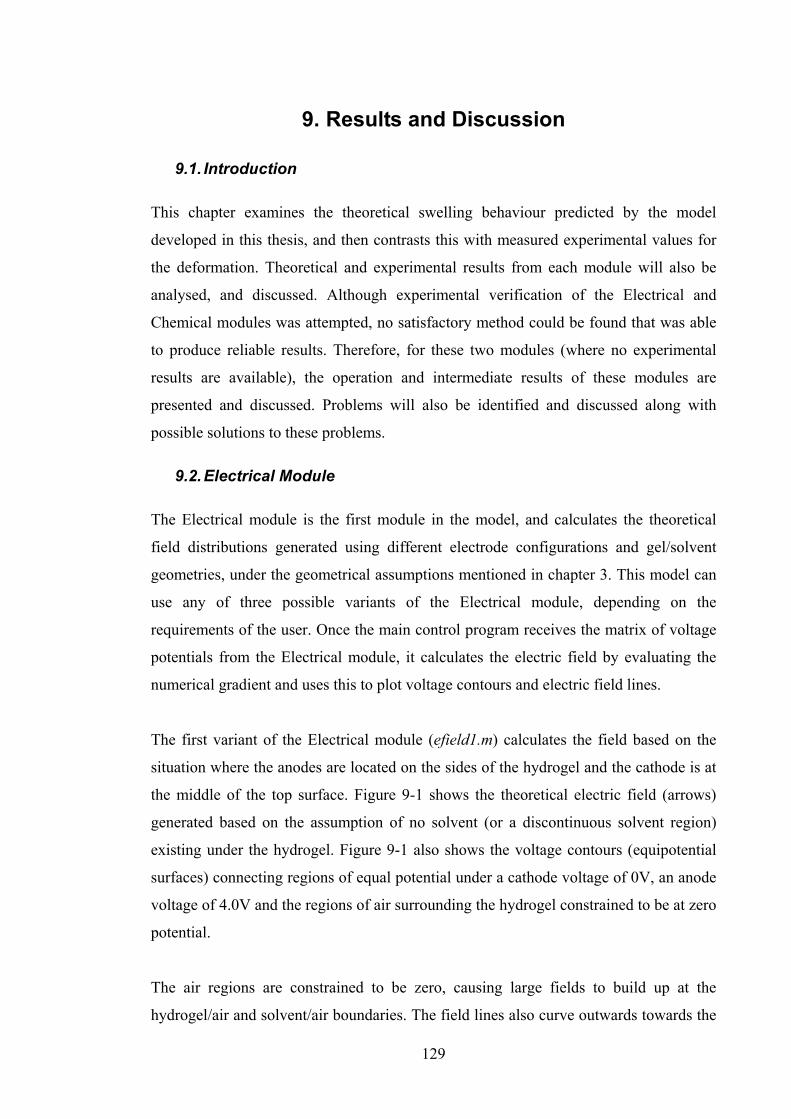
129

9. Results and Discussion

9.1. Introduction

This chapter examines the theoretical swelling behaviour predicted by the model

developed in this thesis, and then contrasts this with measured experimental values for

the deformation. Theoretical and experimental results from each module will also be

analysed, and discussed. Although experimental verification of the Electrical and

Chemical modules was attempted, no satisfactory method could be found that was able

to produce reliable results. Therefore, for these two modules (where no experimental

results are available), the operation and intermediate results of these modules are

presented and discussed. Problems will also be identified and discussed along with

possible solutions to these problems.

9.2. Electrical Module

The Electrical module is the first module in the model, and calculates the theoretical

field distributions generated using different electrode configurations and gel/solvent

geometries, under the geometrical assumptions mentioned in chapter 3. This model can

use any of three possible variants of the Electrical module, depending on the

requirements of the user. Once the main control program receives the matrix of voltage

potentials from the Electrical module, it calculates the electric field by evaluating the

numerical gradient and uses this to plot voltage contours and electric field lines.

The first variant of the Electrical module (efield1.m) calculates the field based on the

situation where the anodes are located on the sides of the hydrogel and the cathode is at

the middle of the top surface. Figure 9-1 shows the theoretical electric field (arrows)

generated based on the assumption of no solvent (or a discontinuous solvent region)

existing under the hydrogel. Figure 9-1 also shows the voltage contours (equipotential

surfaces) connecting regions of equal potential under a cathode voltage of 0V, an anode

voltage of 4.0V and the regions of air surrounding the hydrogel constrained to be at zero

potential.

The air regions are constrained to be zero, causing large fields to build up at the

hydrogel/air and solvent/air boundaries. The field lines also curve outwards towards the

130

bottom of the hydrogel region as current is forced to flow only from the sides of the

hydrogel to the top surface. This also results in the appearance of large fields around the

cathode as current converges to a single point. All of these effects are expected, given

knowledge of the physical geometry of the system.

OOOOOOOOO

OOOOOOOOO

OOOOOOOOO

OOOOOOOOO

OOOOOOOOO

OOOOOOOOO

OOOOOOOOO

OOOOOOOOO

OOOOOOOOO

OOOOOOOOO

OOOOOOOOO

OOOOOOOOO

OOOOOOOOO

OOOOOOOOO

Cathode

Anode

Figure 9-1: Field generated by efield1.m. Numbers in figure in volts.

The second variant of the Electrical module (efield2.m) features an almost identical

geometry to the first variant, except that in this case the solvent is also assumed to be

present under the gel. This solvent layer connects the two anodes on the sides of the gel,

and causes the anode to become almost ‘C’ shaped. As with the first variant of the

Electrical module, the air regions are again constrained to be zero, leading to large fields

at the hydrogel/air and solvent/air boundaries. The curvature of the field lines at the

x

y

131

bottom of the hydrogel is less than for the first variant however, owing to the current

path at the bottom of the hydrogel. As expected, large fields still occur around the

cathode as the current again converges. Figure 9-2 shows an example of an electric field

generated by the second variant of the Electrical module. As with Figure 9-1, this figure

shows the voltage contours connecting regions of equal potential under a cathode

voltage of 0V and an anode voltage of 4.0V.

OOOOOOOOO

OOOOOOOOO

OOOOOOOOO

OOOOOOOOO

OOOOOOOOO

OOOOOOOOO

OOOOOOOOO

OOOOOOOOO

OOOOOOOOO

OOOOOOOOO

OOOOOOOOO

OOOOOOOOO

OOOOOOOOO

OOOOOOOOO

Cathode

Anode

Figure 9-2: Field generated by efield2.m. Numbers in figure in volts.

The Electrical module can also calculate the theoretical potential distribution when a

hard boundary does not exist between the hydrogel/solvent and the air regions

surrounding them. An example of this feature is shown in Figure 9-3 and Figure 9-4.

As expected, in Figure 9-3 the large fields at the hydrogel/air boundary disappear,

x

y

132

which also causes the curvature of the calculated field lines to decrease significantly

from Figure 9-2. The field distribution is again different from the previous variants as

shown in Figure 9-3. As before the cathode voltage is held at 0V and the anode voltage

at 4.0V.

Figure 9-3: Field generated by efield2.m (no constraints). Numbers in figure in volts

The modification of the original Electrical module to include continuous boundaries

arose due to subtle, but important differences between Kirchoff’s current law and

Laplace’s equation. Although electric fields can readily pass between mediums of

different permittivity, at voltages below the breakdown voltage, current will not flow

from a medium of low resistance (such as the hydrogel) into a medium of high

resistance (such the surrounding air). For this reason, current flow ends abruptly at the

hydrogel/air and solvent/air interfaces, which presented a major challenge for this work.

In order to satisfy Laplace’s equation at the boundary, it had to be possible for current to

flow across the boundary. To satisfy Kirchoff’s current law at the boundary, no current

should flow across the boundary. As discussed in chapter 3, this was solved by creating

a one-way current flow. Since no current could ever physically flow from the air into

the hydrogel, current was permitted to flow in this way, but not back into the air (thus

simultaneously satisfying Laplace’s equation and Kirchoff’s current law at the

boundary). Due to the differences in permittivity, the electric field does still change

from the hydrogel into the air region, but to ease the computational requirements of this

x

y

133

initial model, it was decided to assume this change was negligible. Future

improvements to this work will certainly focus on this aspect of the Electrical module or

perhaps a commercial FEM program may be used to calculate the field distributions.

The third variant (efield3.m) of the Electrical module is the one predominantly used in

this work. It consists of an upper electrode (cathode) which mostly covers the top

surface of the hydrogel. The extent of coverage can be adjusted, and in this work is

configured to cover all but the final column of nodes in the hydrogel region

(corresponding to approximately 70%, which matches the experimental conditions). In

Figure 9-4, the cathode voltage is set to 0V and the anode voltage to 1.0V. As in Figure

9-3, the air regions surrounding the hydrogel are not constrained to be at zero potential

and the field is continuous across the gel/air boundary. When the third variant of the

Electrical module was used, the calculated field was again different. Owing to the large

cathode on the top surface of the hydrogel, the curvature of the field lines is

significantly less than for the first two variants (Figure 9-4).

OOOOOOOOO

OOOOOOOOO

OOOOOOOOO

OOOOOOOOO

OOOOOOOOO

OOOOOOOOO

OOOOOOOOO

OOOOOOOOO

OOOOOOOOO

OOOOOOOOO

OOOOOOOOO

OOOOOOOOO

OOOOOOOOO

OOOOOOOOOCathode

Anode

Figure 9-4: Field generated by efield3.m. Numbers in figure in volts

x

y

134

In practice however, it was found that when simulations were conducted using the large

fields calculated by the Electrical module, the model became unstable. The role of the

Electrical module in this instability was confirmed through a rigorous process that

isolated each module in turn and examined its effect on stability. It was found that due

to the relatively small dimensions of the hydrogel, large electric fields were generated

by the Electrical module, which while not affecting the Electrical module, did cause the

Chemical module to become unstable. The nature of this instability will be discussed in

the next section, but its relevance to the Electrical module will be mentioned here.

Because of this instability, the output from the Electrical module had to be scaled to

ensure that no value exceeded 1V cm-1 (a value that was found empirically). While this

will certainly affect the overall output of the model, the addition of this scaling factor

will not alter any trends, which still allows useful information to be derived from this

work.

Another problem with the Electrical module is that the theoretical predictions are

difficult to verify experimentally, particularly with the geometry used in this work.

While the use of a scaling parameter and lack of experimental verification certainly

affects the overall result of the model, the model can still be useful in determining

trends and patterns that occur during swelling. Results from other numerical simulations

can also be used to verify some of the results generated.

Although the ion transport through the hydrogel is not directly simulated by the model,

examination of the experimentally-measured current flowing through the hydrogel can

possibly be used to provide insight into the ion transport mechanisms occurring. A

graph of the average resistance of the hydrogel versus time is shown in Figure 9-5. In

the case of a perfect conductor, one would expect the resistance to be constant over time

and for all applied voltages. From Figure 9-5, it can be seen that the hydrogel is not a

perfect conductor and its resistance rises and falls regularly over time, with the peak-to-

peak value of these oscillations steadily decreasing. This rise and fall in the resistance

(and hence current, since the voltage is constant) seems to indicate a capacitive

charging/discharging effect – something mentioned by other authors working with

poly(acrylic acid) (such as Shahinpoor). Although more data is required to conclude that

the resistance of the hydrogel is converging, the general trend certainly appears to

suggest that this is possibly the case. The calculated resistance values are also

135

significantly higher than expected, but this most probably results from poor contact

between the hydrogel and electrodes.

As expected, due to the increased current flowing through the gel, the resistance values

for 7.5V are higher than those for 5V. The data for 10V is anomalous however, and is

lower than for 7.5V. This suggests that between 7.5V and 10V, Ohm’s law becomes

invalid for the hydrogel material, and the simple analysis applied here is no longer

applicable (see Figure 9-5). In any event, more study needs to be made of the current

flow to assert the validity of the above observations. A complete set of data is given in

Appendix A.

Overall, the results from this section are encouraging and do offer reasonable

predictions for the potential distribution in the hydrogel region using different

electrode/hydrogel/solvent geometries. A major advantage of the modular design used

in this work is that the Electrical module can be run completely independently. This

allows a user to generate a library of voltage potentials for different electrode

configurations, and then test these on hydrogels with different parameters.

136

020406080100

120

140

060

120

180

240

Tim

e (s

)

Resistance (Ω)

5V 7.5V

10V

Figu

re 9

-5: A

vera

ge r

esis

tanc

e of

hyd

roge

l ove

r tim

e (d

otte

d lin

es a

dded

to a

id th

e ey

e)

137

9.3. Chemical Module

The Chemical module is the second module in the overall model, and also provides the

main engine to the model. In its current incarnation, the Chemical module is the first

module in the time loop, and therefore possibly the most important module in the

overall model. Ion and water movement through the hydrogel from the solvent is

responsible for the creation of the forces that act to deform the hydrogel. As discussed

in chapter 4, the Chemical module is responsible for two aspects of the overall model –

the initial ion distribution in the hydrogel and solvent regions, and the ion transport

through the hydrogel.

An example of a generated initial ion distribution in the hydrogel is shown in Figure

9-6. This information is calculated outside the main time loop by two smaller scripts

that pass their results to the main part of the Chemical module for use. This module

calculates the initial ion distribution based on Coulombic and Lennard-Jones (L-J)

interactions, which differs from some models where a uniform ion distribution is

assumed to exist. In practice however, it was found that this model produced similar

results when using either a uniform or calculated initial ion distribution, indicating that

the initial ion distribution may be less important than first thought. Since the initial ion

distribution can be calculated prior to running the overall model, Coulombic and L-J

interactions can be used without adversely affecting the overall run time of the model.

Although other physical interactions also occur (such as Van der Waals forces), this

model only considers the Coulombic and L-J interactions as these are considered to be

the dominant influences in the initial ion distribution. The Coulombic interaction

accounts for the behaviour of charged species in a confined space, while the L-J

interaction stipulates the minimum distance two ions can be to each other. Another

advantage of the modular design of this model is that additional interactions can be

added at a later time, if required.

138

Figure 9-6: Possible ion distribution in hydrogel region, 50 ions on a 100x100 grid

As expected, using this approach causes negative and positive ions to cluster together,

and then the groups of ions try to move as far apart from other pairs as possible. This

results in pairs of ions appearing at uniform distances along the outside of the hydrogel

region, while the middle of the hydrogel region has ion pairs scattered randomly

throughout. The ion distribution along the edges of the hydrogel region is to be

expected, and in fact is mentioned by Limbach and Holm [108] in their modeling of

DNA chains, and the distribution in the middle of the hydrogel is similar to that

obtained when using a uniform ion distribution. Although the ion pairs in Figure 9-6

appear to overlap, this is merely a by-product of the axis scale used.

There are also some potential sources of error in this part of the Chemical module.

Some of the constants for poly(acrylic acid) hydrogels used by the module to calculate

L-J and Columbic potentials could not be obtained and in these cases, the corresponding

constants for water were assumed to be satisfactory. Since the L-J interaction is

predominantly used to ensure ions do not move closer than their physical radii will

allow, using the values of water for the constants may force the ions to move further

from each other than actually occurs. Since the poly(acrylic acid) hydrogels used in this

work do consist predominantly of water however, it is expected that any errors resulting

from the use of water constants will be minimal.

hydrogel

solvent

139

A more significant problem in this module is that the initial ion concentration in the

hydrogel is calculated using static conditions. Once an ion is placed into the system, its

position is used to calculate the positions of all of the ions placed subsequently. This

static approach is the cause of the single ion in the centre-left of Figure 9-6. One

advantage of using a static approach however, is that it allows the model to use “one-to-

many” calculations (where one equation is compared against many). The number of

equations grows linearly as the number of ions in the system is increased, which allows

control over the total calculation time. This module also does not consider the

generation or recombination of ion pairs and any long distance screening effects, which

may prove significant. In reality, each ion dynamically redistributes itself based on the

locations of all the other ions. This is an example of a “many-to-many” problem, which

cannot easily be solved in a reasonable amount of time. Ions also combine with each

other, and new ions are spontaneously generated, which further complicates the

calculations.

Another potential problem is that if the number of elements is significantly low, the

model cannot provide reasonable results. For example, if a one-dimensional distance of

1cm was divided amongst 5 elements, each element would be 0.2cm apart. If a positive

ion was initially placed at the origin, the model would attempt to place a negative ion as

close as possible to the origin (owing to Coulombic attraction). A L-J interaction would

prevent the negative ion from being placed directly on the positive ion however, and so

the negative ion would be placed 0.2cm from the positive ion – clearly, an unphysical

result. To combat this, a user can input a “resolution factor” which attempts to create a

more realistic situation. For example, if a resolution factor of 1000 was used the model

would divide 1cm into 5 × 1000 = 5000 elements, with each element then being

0.001cm apart. By increasing the number of elements the operation speed of this part of

the Chemical module decreases, but as discussed previously, this is not necessarily

critical.

Although calculating the initial ion distribution is one function of the Chemical module,

its main function is to calculate the change in the concentration of each ionic species in

the system in both space and time. The main equation in the Chemical module is

equation (4.34), which includes terms to describe both the diffusive (1st term) and

migrative (2nd term) flux through the hydrogel for each species.

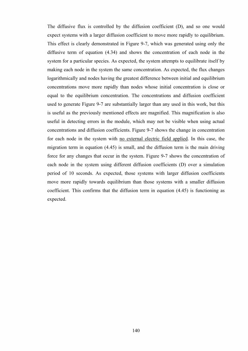
140

The diffusive flux is controlled by the diffusion coefficient (D), and so one would

expect systems with a larger diffusion coefficient to move more rapidly to equilibrium.

This effect is clearly demonstrated in Figure 9-7, which was generated using only the

diffusive term of equation (4.34) and shows the concentration of each node in the

system for a particular species. As expected, the system attempts to equilibrate itself by

making each node in the system the same concentration. As expected, the flux changes

logarithmically and nodes having the greatest difference between initial and equilibrium

concentrations move more rapidly than nodes whose initial concentration is close or

equal to the equilibrium concentration. The concentrations and diffusion coefficient

used to generate Figure 9-7 are substantially larger than any used in this work, but this

is useful as the previously mentioned effects are magnified. This magnification is also

useful in detecting errors in the module, which may not be visible when using actual

concentrations and diffusion coefficients. Figure 9-7 shows the change in concentration

for each node in the system with no external electric field applied. In this case, the

migration term in equation (4.45) is small, and the diffusion term is the main driving

force for any changes that occur in the system. Figure 9-7 shows the concentration of

each node in the system using different diffusion coefficients (D) over a simulation

period of 10 seconds. As expected, those systems with larger diffusion coefficients

move more rapidly towards equilibrium than those systems with a smaller diffusion

coefficient. This confirms that the diffusion term in equation (4.45) is functioning as

expected.

141

Figu

re 9

-7: E

ffec

t of d

iffus

ion

coef

ficie

nt o

n di

ffus

ion

rate

Nod

e w

ith h

igh

initi

al c

once

ntra

tion

Nod

e w

ith lo

w in

itial

con

cent

ratio

n

Tim

e

Tim

e

Tim

e

(s)

(s)

(s)

142

To examine the effect of the migrative term in equation (4.34), a similar procedure to

that discussed for the diffusive term is used. The behaviour of the Chemical module

with and without the presence of an external electric field is shown in Figure 9-8 and

Figure 9-9. Under the influence of an external electric field, ions should migrate through

the solvent and hydrogel regions dependending on their valence and the polarity of the

electrodes. This should cause a higher than normal concentration of these ions at some

point in the system. Figure 9-8 shows the concentrations of all nodes in the hydrogel

with no external electric field and the surrounding solvent concentration is held constant

at 0.045mol L-1. Figure 9-9 shows the identical situation with an external electric field

applied.

These results appear as an inversion of those shown in Figure 9-7, since in the case of

Figure 9-8 and Figure 9-9, the initial concentration of each node is set to be zero. The

concentration of the surrounding solvent is fixed at 0.045mol L-1, which results in ions

flowing from the solvent region into the hydrogel region. With no electric field present

(Figure 9-8), the situation is identical to the results obtained in Figure 9-7. Ions move

from the solvent into the hydrogel in an attempt to equilibrate the concentration with the

concentration of the surrounding solvent. Due to the large excess of solvent, the

concentration is assumed not to change appreciably as diffusion occurs from the

solvent. When an external electric field is applied however (Figure 9-9), the situation

changes dramatically. As in Figure 9-8, flux occurs in order to bring the nodes

originally at zero up to the concentration of the solvent. When this concentration is

reached however, the flux does not stop as in Figure 9-7 and Figure 9-8. Rather, ions

continue to diffuse into the different nodes giving them a concentration higher than that

of the surrounding solution. The flux does steadily decrease however, and eventually

becomes constant, but at a concentration significantly higher than the surrounding

solvent. The exact reason for the concentration becoming constant is unknown, but

probably results from the way the Chemical and Electrical modules interact. The effects

shown in Figure 9-9 do offer clear proof however of the effect of applying an external

electric field on the Chemical module.

143

Figure 9-8: Concentration of nodes with no external electric field applied

Figure 9-9: Concentration of nodes with external electric field applied

Time (s)

Time (s)

Con

cent

ratio

n (m

ol L

-1)

Con

cent

ratio

n (m

ol L

-1)

Concentration of surrounding solvent

Concentration of surrounding solvent

144

Lastly, it is important to discuss the stability of the Electrical and Chemical modules.

During operation, it was noticed that occasionally the concentration of one or more

elements in the Chemical module would rapidly rise to infinity, causing the module

(and overall model) to become unstable. The exact start time of this instability was

random and grew rapidly once initiated. However, this instability, while concerning,

does not suggest any great error in this model or indeed with the overall approach

followed in this work. The most likely cause is the order in which the Chemical module

performs the different calculations. A relatively minor change in the order of the

calculations could cause the overall model to divide or multiply by either zero or

infinity leading to model instability. In this case, the exact cause of the instability could

be extremely difficult to trace.

To verify the origin of this instability, each module in the overall model was isolated

and tested in the order of operation until the instability was located. Fortunately, the

instability was found to first occur in the Chemical module, and thus it was only

necessary to examine two of the five overall modules (the Electrical and Chemical

modules). Since the Electrical module does not appear within the time loop, and the

instability appears to be time-dependent, the most likely source of the instability was

somewhere in the Chemical module. To find the cause of this instability, it was thought

useful to examine the long-time behaviour of the total ion concentration in the system.

The premise behind this argument is that the cause of the instability may be periodic,

and only occur with some iterations – by examining which iterations, clues may be

gained as to the exact location of the problem. To examine the long-time behaviour, the

Chemical module was given a non-uniform initial ion distribution and was allowed to

equilibrate over time. The system was closed, and as such, the total concentration in the

system should not change as the concentration of each element moves towards

equilibrium. Any instability would appear as sharp spikes in the total concentration as

the model was run. The total concentration of the system is shown in Figure 9-10.

145

Figure 9-10: Stability of total concentration

As can be seen from the figure, the overall ion concentration does not change

significantly over 5,000 iterations. In fact, the total concentration decreases by

approximately 0.008% between the 500th and 5000th iteration, and there are no

anomalous spikes present anywhere in the graph. Since the error does not appear to be

inherent to the Chemical module, the other most likely source is that it is carried into the

Chemical module from the Electrical module.

After more exhaustive testing, the most probable source of the instability was identified

as being related to the method that the Chemical module used when handling input from

the Electrical module. When the Chemical module was passed the value of the electric

field calculated by the Electrical module, the instability mentioned previously would

occur. When the maximum value of the electric field was reduced so that no point

exceeded 1V cm-1, no instability occurred. This upper bound offers further proof that a

“divide-by-zero” error is responsible for the model instability, as repeated division by a

number greater than one can rapidly cause the quotient to drop to zero – if this number

was then used as a divisor, the overall result would be infinite.

Iteration

To

tal C

once

ntra

tion

(mol

L-1)

146

It is important to realise however, that the tests performed in this work to verify the

location of the instability are inconclusive – it is entirely possible that the applied

electric field is coupled to another variable in the Chemical module which is ultimately

responsible for the instability. Lowering the magnitude of the electric field may prevent

this variable from causing instability, but a very real threat to the overall model may

still remain. While scaling the output of the Electrical module will certainly affect the

overall output of the model, any trends that occur will still be visible and can be used to

gather useful information on the gel swelling process. Another point is that since

MATLAB can easily handle the concepts of zero and infinity, locating a “divide-by-

zero” error can be extremely cumbersome. When this model is compiled into C or

FORTRAN, it is expected that the source of the instability will become apparent, as

these languages do not tolerate “divide-by-zero” errors.

The overall aim of this work however, was to create a general framework for an overall

model to describe the swelling of polymer hydrogels under the influence of an electric

field. Although the Chemical module is not yet functioning perfectly, it is expected that

the minor bugs still present will be easily removed by future work.

9.4. Force Module

The Force module is the third module in the overall model, and is also the first where

experimental data can be collected and compared against the theoretical predictions

made by the overall model. As discussed in section 9.3, the use of a scaling parameter

means that overall values cannot be directly compared, however trends between the

theoretical and experimental data will be identified and examined. The output of the

Force module is the force applied to each node in the hydrogel system for each timestep.

Experimentally, it is impossible to measure the force on individual parts of the

hydrogel, as the mere act of measurement creates forces which alter the forces on other

parts of the gel. To counter this, the overall pressure on the upper surface of the

hydrogel (with the bottom constrained) was measured. The edges of the hydrogel were

free to expand or contract and this causes the overall measured force to be lower than if

the edges were also constrained. A comparison of the experimental and theoretical total

force generated is shown in Figure 9-11. A complete set of data is given in Appendix A.

Two features are immediately apparent in Figure 9-11 when the experimental data is

examined. Firstly, the amount of force generated by the hydrogel as it swells is very

147

small. However, as previously mentioned, the edges of the hydrogel are not constrained

in this setup, allowing energy to be lost through the sides of the hydrogel. It is likely

that a greater force could be generated by the top surface if the sides were constrained,

but this assumption was not verified. The second interesting feature of the experimental

data is the appearance of an upper bound for the generated force. Both sets of

experimental data grow linearly for the first 40s, and then begin to move asymptotically

towards some maximum force. This maximum force is between 100mN and 110mN for

both sets of data and results from the finite elasticity of the hydrogel. As the force

generated expands the hydrogel, an elastic restoring force is also developed. If one

assumes linear elasticity, this force grows as the square of the deformation, and very

rapidly becomes equal to the generated force. Once these forces match each other, no

further deformation occurs and the generated force becomes constant.

The theoretical predictions made by this model differ from those recorded

experimentally. As with the experimental data, the theoretical data will be discussed in

the context of two key parameters: the amount of force generated and the trend of the

generated force. In this work, the Force module predicts that the swelling force on the

upper surface of the hydrogel climbs from approximately 60mN to 70mN over a period

of 100s - significantly lower than the experimentally measured force of 110-120mN.

This phenomenon can be explained however, when one recalls that the difference most

probably results from the scaling of the electric field (as discussed in section 9.3). When

the full results from the Electrical module can be used in the Chemical module, it is

expected that a force closer to the experimentally-measured values will be achieved.

The second feature of the data predicted by the model is that it follows a linear trend,

and not the polynomial trends followed by the experimental data. This trend can be

explained however, when one considers the modular approach followed in this work. In

the experimental data, the swelling force decreases in response to an elastic restoring

force. In the theoretical model, the elastic restoring force is calculated by the

Mechanical module and so is not available to the Force module. As such, the forces

generated by the Force module are only one part of the total force experienced by the

hydrogel – the Mechanical module provides the elastic restoring force at a later stage

and the combination of these forces provides the net force on the hydrogel. This

unfortunately does question the validity of using a sequential model; however in the full

model (with all the modules operating together) all of the calculated forces are

148

available. One possible solution to this problem is the use of a feedback loop between

the Force and Mechanical modules, which is left as a future development on this model.

The amount of force generated by the hydrogel is not critical to the operation of this

model, but is important when considering the overall design of a hydrogel lens system.

The low amount of force generated requires that flexible, easily deformable materials be

used to encase the hydrogel to allow the hydrogel to deform under the influence of an

electric field.

Forc

e ge

nera

ted

unde

r 5V

DC

0

0.02

0.04

0.06

0.080.1

0.12

0.14

020

4060

8010

012

0

Tim

e (s

)

Force (N)

Test

1

Test

2

Theo

retic

al

Poly

. (Te

st 2

)

Poly

. (Te

st 1

)

Line

ar (T

heor

etic

al)

Figu

re 9

-11:

For

ce g

ener

ated

by

uppe

r su

rfac

e of

hyd

roge

l

149

9.5. Mechanical Module

Recall from chapter 6 that the Mechanical module takes as its input the force on each

node as calculated by the Force module. The Mechanical module then calculates the

deformation of each node in the hydrogel based on the assumptions of linear elasticity

with no hysteresis. Although deformation data is calculated for each node in the

system, in this work we are particularly interested in the deformation of the nodes on

the upper surface of the gel. In particular, the deformation of the upper left, centre and

right nodes (as discussed in chapter 8).

To generate the theoretical results for this module, the output of the Mechanical module

was recorded and analysed for two variants of the Electrical module under varying

applied voltages. Recall from earlier discussion, that the different variants of the

Electrical module correspond to different electrode configurations, and so it is

interesting to examine what (if any) effects each variant has on the predicted

deformation of the hydrogel. The sampling interval was chosen as 30s, to coincide with

the experimentally-measured deformation, and the results are shown in Figure 9-12 to

Figure 9-14.

In all three figures, the deformation produced by using the second variant of the

Electrical module far exceeds the deformation generated using the third variant. This is

most probably due to the wider surface area of the cathode used in the third variant

reducing the overall deformation of the top surface. For all three applied voltages, the

Mechanical module also predicts an asymptotic swelling towards some maximum

deformation, but this is expected when one considers the asymptotic nature of the

applied force.

150

0.00

0.05

0.10

0.15

0.20

0.25

0.30

0.35

030

6090

120

150

180

210

240

270

300

Tim

e (s

)

Deformation (mm)

5V -

Varia

nt 2

7.5V

- Va

riant

210

V - V

aria

nt 2

5V -

Varia

nt 3

7.5V

- Va

riant

310

V - V

aria

nt 3

Figu

re 9

-12:

The

oret

ical

def

orm

atio

n of

upp

er c

entr

e no

de

151

0.00

0.10

0.20

0.30

0.40

0.50

0.60

0.70

0.80

030

6090

120

150

180

210

240

270

300

Tim

e (s

)

Deformation (mm)5V

- Va

riant

2

7.5V

- V

aria

nt 2

10V

- Var

iant

2

5V -

Varia

nt 3

7.5V

- V

aria

nt 3

10V

- Var

iant

3 Figu

re 9

-13:

The

oret

ical

def

orm

atio

n of

upp

er le

ft n

ode

152

0.00

0.10

0.20

0.30

0.40

0.50

0.60

030

6090

120

150

180

210

240

270

300

Tim

e (s

)

Deformation (mm)

5V -

Varia

nt 2

7.5V

- Va

riant

210

V -

Var

iant

25V

- Va

riant

37.

5V -

Varia

nt 3

10V

- V

aria

nt 3

Figu

re 9

-14:

The

oret

ical

def

orm

atio

n of

upp

er r

ight

nod

e

153

When the deformation of the centre node is examined (Figure 9-12), it can be seen that

the swelling rate of the hydrogel remains almost constant under all applied voltages.

This is contrary to the expected behaviour, as the swelling rate of hydrogels generally

increases with increasing voltage (as reported by other authors, e.g. Salehpoor [66]).

The absolute deformation does increase with increasing voltage however, which is

unexpected since deformation is generally considered to be independent of applied

voltage. After 300 seconds, using the second variant, the Mechanical module predicts a

maximum deformation of 0.28mm (5V), 0.31mm (7.5V) and 0.33mm (10V) for the

centre of the hydrogel. The maximum deformation predicted using the third variant is

0.04mm for all applied voltages.

The deformation of the left and right edges of the hydrogel (Figure 9-13 and Figure

9-14) display similar trends to the centre node, except that the Mechanical module

predicts the deformation to decrease with increasing voltage – in direct contrast to the

predicted deformation of the centre. The predicted deformation of the left edge using the

second variant is 0.75mm (5V), 0.63mm (7.5V) and 0.56mm (10V). Using the third

variant, a deformation of 0.11mm (5V), 0.10mm (7.5V) and 0.09mm (10V) is predicted.

Similar deformation occurs for the right edge of the hydrogel. Using the second variant,

the Mechanical module predicts a deformation of 0.53mm (5V), 0.45mm (7.5V) and

0.39mm (10V); a deformation of 0.08mm (5V), 0.07mm (7.5) and 0.06mm (10V) is

predicted when the third variant is used. These results are interesting, as they suggest

that the deformation of the hydrogel edges will be substantially larger than the

deformation of the centre, even though most of the current is focused on that region.

To verify these predictions, the results predicted by the Mechanical module need to be

compared to the experimental results. Figure 9-15 to Figure 9-17 show the

experimentally-measured deformation of the centre, left and right edges of the hydrogel

under an applied electric field of 5, 7.5 and 10V DC.

Each experiment was run numerous times, with three “good” experiments for each

applied voltage being chosen for verification purpose. In some cases, significantly more

than three “good” data sets were available, but to ensure consistency between

experiments, only three data sets were used. In this work, a “good” experiment was

defined as one where the deformation of the hydrogel was clearly captured on film and

154

which did not have significant artifacts present (such as changing shadows and stray

reflections).

One major difference between the theoretical and experimental data is that the

experimentally-measured deformation follows a linear trend, while the deformation

predicted by this theoretical model follows a polynomial trend. The deformation of the

centre node predicted by the model is also significantly less than that measured

experimentally. There are numerous possible reasons for this discrepancy, but two of

the most probable causes are the use of incorrect material parameters in the overall

model and the scaling of the applied electric field. It is possible that the weight of the

cathode also has some effect on the results.

Experimentally it is observed that the deformation and swelling rate of the centre

increases with increasing voltage, which is similar to the behaviour predicted by the

Mechanical module. Experimentally, it is observed that the absolute deformation of the

centre increases with increasing voltage which is also predicted by the Mechanical

module. It is also observed that under 10V the rate of swelling is almost double that

under 5V. There is almost no difference in the swelling rate between 5V and 7.5V

however, indicating that some change in the hydrogel occurs between 7.5V and 10V.

This compares against an almost constant swelling rate predicted by the Mechanical

module.

The most notable difference between the theoretical predictions and the experimental

results occurs however, when the deformation of the left and right edges of the hydrogel

is examined (Figure 9-16 and Figure 9-17). In both cases, the Mechanical module

predicts deformation in the positive y-direction (upwards), but experimentally

deformation occurs in the negative y-direction (downwards)! There are many possible

causes for this behaviour, but the most likely is that some kind of physical obstruction

blocks the upwards movement of the hydrogel edges. Since the sides of the gel are not

constrained, the only possible cause of a physical obstruction is the cathode placed over

the surface. As discussed in the experimental design (chapter 8), the cathode was

carefully designed to minimise any loading onto the hydrogel surface. It is possible

however, that due to the small forces generated by the hydrogel, the cathode may still be

too restrictive. Future developments of this work may be forced to seek an alternative

155

method of attaching the cathode to the surface, or possibly working with significantly

thinner and lighter materials.

156

y =

0.00

156x

+ 0

.084

79y

= 0.

0015

8x +

0.0

5453

y =

0.00

302x

+ 0

.107

56

-0.20.0

0.2

0.4

0.6

0.8

1.0

1.2

030

6090

120

150

180

210

240

270

300

Tim

e (s

)

Deformation (mm)

5V 7.5V

10V

Line

ar (5

V)

Line

ar (7

.5V

)Li

near

(10V

)

Figu

re 9

-15:

Exp

erim

enta

l def

orm

atio

n of

upp

er c

entr

e no

de

157

y =

-0.0

02x

+ 0.

0725

y =

-0.0

009x

- 0.

2568

y =

-0.0

011x

- 0.

7082

-2.0

-1.5

-1.0

-0.50.0

0.5

030

6090

120

150

180

210

240

270

300

Tim

e (s

)

Deformation (mm)

5V 7.5V

10V

Line

ar (5

V)

Line

ar (7

.5V

)Li

near

(10V

)

Figu

re 9

-16:

Exp

erim

enta

l def

orm

atio

n of

upp

er le

ft n

ode

158

y =

-0.0

035x

+ 0

.024

5y

= -0

.002

4x -

0.20

58y

= -0

.001

3x -

0.18

98

-1.4

-1.2

-1.0

-0.8

-0.6

-0.4

-0.20.0

0.2

030

6090

120

150

180

210

240

270

300

Tim

e (s

)

Deformation (mm)

5V 7.5V

10V

Line

ar (5

V)

Line

ar (7

.5V

)Li

near

(10V

)

Figu

re 9

-17:

Exp

erim

enta

l def

orm

atio

n of

upp

er r

ight

nod

e

159

One interesting observation concerning Figure 9-16 and Figure 9-17 is that the absolute

deformation of the edges increases with increasing voltage, but the swelling rate

decreases with increasing voltage. This is similar to the behaviour predicted by the

Mechanical module, and opposite to the behaviour of the centre of the hydrogel. This

suggests that there may exist a finite amount of energy available for swelling. If the

majority of this energy was used to deform the centre of the hydrogel (for example

under 10V), not much energy is available to deform the edges of the hydrogel (leading

to a correspondingly low edge deformation).

The experimentally-measured deformation of the left edge was -0.7mm (5V), -0.5mm

(7.5V) and -0.8mm (10V). This is compared to the predicted deformation values of

0.75mm (5V), 0.63mm (7.5V) and 0.56mm (10V). The larger deformation of the right

edge under 10V appears to be anomalous, as this is the only measurement where a

larger voltage caused a larger deformation. The experimentally-measured deformation

of the right edge was -1.2mm (5V), -0.8mm (7.5V) and -0.5mm (10V), which is also

compared to the predicted deformation of 0.53mm (5V), 0.45mm (7.5V) and 0.39mm

(10V). As predicted by the Mechanical module, the largest deformation of the edges

occurs when the lowest voltage is applied.

The difference in deformation direction most probably occurs as a result of the

movement of nodes in the y-direction. This effect is not considered by the Mechanical

module, and if the edges were constrained, it is likely that the nodes at the edge of the

hydrogel would move in an upwards direction (as predicted by the Mechanical module).

Overall, the general predictions made by the Mechanical module do not appear to

coincide with the measured experimental deformation! The most probable cause of this

discrepancy is the inaccuracy of the experiemental data, although bugs in the model

may also be a factor. Once more precise measurements of the material parameters are

made and any effects from the cathode is removed, it is hoped that closer agreement will

occur between the experimental and theoretical results.

9.6. Optical Module

The Optical module receives as input the deformation data shown in Table 11-4 and

Table 9-3. As discussed in chapter 7, the module then fits this data to either a parabolic

or circular line, and uses this shape to determine the resulting change in focal length.

The focal length data is calculated using equations (7.1), (7.3) and (7.4) for both a

160

paraboloidal and a spherical fit. A comparison of the predicted focal length for each of

the applied voltages (5V, 7.5V and 10V) versus time is shown in Figure 9-18 to Figure

9-20. For each of the graphs, the two theoretical focal lengths generated by the two

variants of the Electrical module are compared with the experimental values. Since the

difference between the parabolic and spherical fits is quite small, the graphs are plotted

using the parabolic fit data. Since the experimentally-measured deformation occurs in

the opposite direction to the theoretically-predicted deformation, the sign of focal length

is also negative. Once the experiemental techniques used in this thesis are improved, it

is expected that the sign of the experimental and theoretical focals will match.

Under both a 5V and 7.5V field, the trends of the theoretically predicted focal length

from the second variant of the Electrical module and the experimentally-determined

focal length are very similar. Both exhibit almost the same initial change in focal length,

and both display a decreasing trend as time increases. The experimental data for 10V is

extremely low however, which again suggests that some significant change occurs in

the swelling mechanisms when the voltage is increased from 7.5V to 10V.

The change in the theoretical focal length generated by the third variant of the Electrical

module is similar to that generated by the second variant, except that the initial change

in focal length is significantly lower. This is due to the smaller deformation calculated

by the third variant, which results in a large initial focal length, and less variation in that

focal length.

Another point of interest is that the theoretical focal length of the third variant appears

to increase after 240 seconds. This may result from an elastic restoring force in the

hydrogel attempting to restore the initial flat surface of the gel discs. Although it is

unclear why such behaviour may occur, it is thought that it may result from the wider

cathode area used in the third variant of the Electrical module. Future work will need to

examine the exact cause of this behaviour.

161

Although the refractive index is not used directly in this model, it is crucial to the

development of a hydrogel lens. Several refractive index measurements were made on

different gel samples, prior to swelling and are listed in Table 9-1. Unfortunately,

during swelling the gel became slightly opaque which prevented accurate post-swelling

refractive index measurements from being made. It is suspected that the NaCl salt forms

in the hydrogel during swelling, and this is clearly a concern for the future development

of a hydrogel lens.

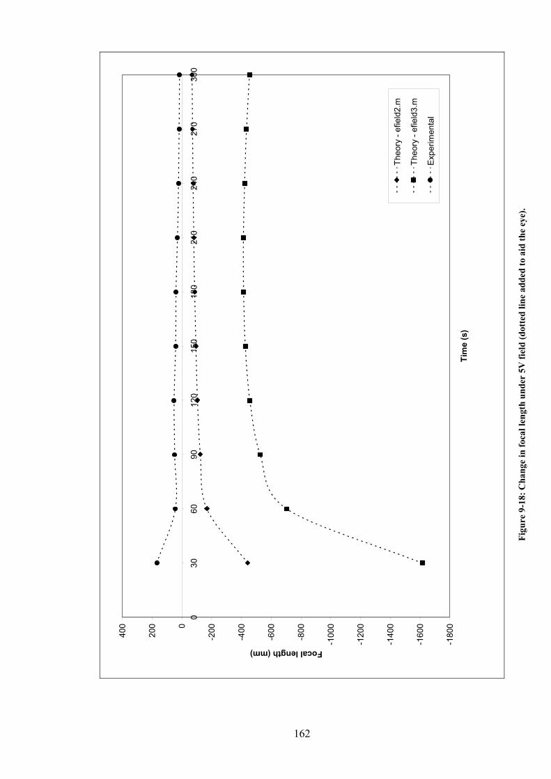
162

-180

0

-160

0

-140

0

-120

0

-100

0

-800

-600

-400

-2000

200

400

030

6090

120

150

180

210

240

270

300

Tim

e (s

)

Focal length (mm)

Theo

ry -

efie

ld2.

m

Theo

ry -

efie

ld3.

m

Exp

erim

enta

l

Figu

re 9

-18:

Cha

nge

in fo

cal l

engt

h un

der

5V fi

eld

(dot

ted

line

adde

d to

aid

the

eye)

.

163

-220

0

-170

0

-120

0

-700

-20030

0

800

1300

1800

030

6090

120

150

180

210

240

270

300

Tim

e (s

)

Focal length (mm)

Theo

ry -

efie

ld2.

m

Theo

ry -

efie

ld3.

m

Exp

erim

enta

l

Figu

re 9

-19:

Cha

nge

in fo

cal l

engt

h un

der

7.5V

fiel

d (d

otte

d lin

e ad

ded

to a

id th

e ey

e).

164

-180

0

-160

0

-140

0

-120

0

-100

0

-800

-600

-400

-2000

200

030

6090

120

150

180

210

240

270

300

Tim

e (s

)

Focal length (mm)

Theo

ry -

efie

ld2.

m

Theo

ry -

efie

ld3.

m

Expe

rimen

tal

Figu

re 9

-20:

Cha

nge

in fo

cal l

engt

h un

der

10V

fiel

d (d

otte

d lin

e ad

ded

to a

id th

e ey

e).

165

Table 9-1: Refractive index of hydrogel

Sample Refractive index (± 0.01)

1 1.35 2 1.36 3 1.36 4 1.33 5 1.34

MEAN 1.35

As shown in Table 9-1, when the refractive index of the hydrogel was measured, an

average value of 1.35 was obtained. This is within the expected range, since the

refractive index of AAC is 1.42 [133], while the refractive index of water is 1.33 [103].

Given that the PAAC hydrogel consists mainly of water, it is expected that the

refractive index will be closer to water than to AAC. Future development will hopefully

attempt to improve this refractive index, and move it closer to the refractive index of

glass (1.5) or possibly some types of plastic.

9.7. Overall Model

While there is still some variance between the experimentally-measured results and the

theoretically-predicted results, the overall trends displayed by the model are

encouraging. The model predicts that the swelling rate of the gel edges should decrease

with increasing voltage, and this is observed experimentally. Once accurate material

properties are available for the hydrogel used in this work, and the instability in the

Electrical module is located, the model should be able to provide definite insights into

the swelling deformation of PAAC hydrogels.

166

10. Conclusion

This work represents the first stage of the development of a computer model to describe

the swelling of polymer hydrogels under the influence of an external electric field.

Although, the specific aim of this work is the development of a model for optical

applications, this work could be readily adapted to other hydrogel applications. From

chapter 2, recall that this model had four overall objectives:

1. Provide results which are useful in determining the effect of different

experimental setups including electrode placement, applied electric field, gel

composition and solvent composition.

This is the most important objective, and possibly also the hardest to quantify. While

the model is not yet fully capable of providing details on the full effects of different

experimental setups, it is certainly capable of demonstrating general effects. The model

allows a user complete control over a myriad of different system parameters, including

electrode geometry, solvent concentration and material properties. Although many of

the modules that comprise this work are still at the early stages of development, it is

expected that as these are developed, the overall power of this model will improve.

2. Consist of individual pieces that allow individual parts of the model to be

adjusted and improved as necessary. Ideally, each part of the model should also

be able to function independently to allow verification of each individual part.

The modular approach followed in this work is a direct consequence of this

requirement, and intermediate results are available to the user. This allows problems

with this work to be readily identified and hopefully solved. Most importantly, minor

modifications are neccessary to enable each module to function independently, if

required.

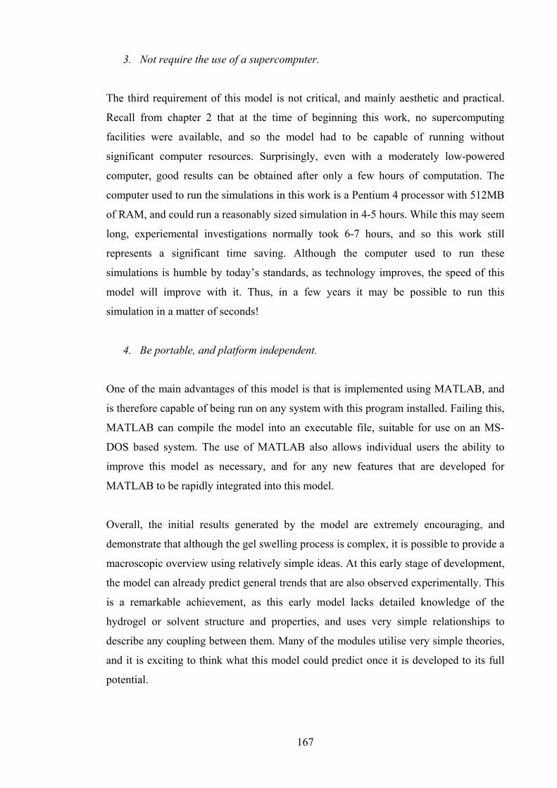
167

3. Not require the use of a supercomputer.

The third requirement of this model is not critical, and mainly aesthetic and practical.

Recall from chapter 2 that at the time of beginning this work, no supercomputing

facilities were available, and so the model had to be capable of running without

significant computer resources. Surprisingly, even with a moderately low-powered

computer, good results can be obtained after only a few hours of computation. The

computer used to run the simulations in this work is a Pentium 4 processor with 512MB

of RAM, and could run a reasonably sized simulation in 4-5 hours. While this may seem

long, experiemental investigations normally took 6-7 hours, and so this work still

represents a significant time saving. Although the computer used to run these

simulations is humble by today’s standards, as technology improves, the speed of this

model will improve with it. Thus, in a few years it may be possible to run this

simulation in a matter of seconds!

4. Be portable, and platform independent.

One of the main advantages of this model is that is implemented using MATLAB, and

is therefore capable of being run on any system with this program installed. Failing this,

MATLAB can compile the model into an executable file, suitable for use on an MS-

DOS based system. The use of MATLAB also allows individual users the ability to

improve this model as necessary, and for any new features that are developed for

MATLAB to be rapidly integrated into this model.

Overall, the initial results generated by the model are extremely encouraging, and

demonstrate that although the gel swelling process is complex, it is possible to provide a

macroscopic overview using relatively simple ideas. At this early stage of development,

the model can already predict general trends that are also observed experimentally. This

is a remarkable achievement, as this early model lacks detailed knowledge of the

hydrogel or solvent structure and properties, and uses very simple relationships to

describe any coupling between them. Many of the modules utilise very simple theories,

and it is exciting to think what this model could predict once it is developed to its full

potential.

168

Many of the recommendations for improving this model have already been discussed,

either in the specific chapter on that part of the model, or in the discussion that

followed. This is the most logical place to mention any future improvements, as these

are then able to be viewed in context with the supporting evidence in close proximity.

It is important however, to highlight some of the more critical problems with this model

that require attention before any additional improvements are made.

1. The most critical problem in this work is the cause of the instability somewhere

in the Electrical or Chemical module. While the cause is almost certainly a

minor error at some stage of the programming, its effect on the overall model is

detrimental. Although several attempts have been made in this work to isolate

the exact location and nature of this error, the exact source remains unclear and

the results are inconclusive.

2. There are also two main improvements that need to be made to the experimental

procedure followed in this work. Firstly, the exact effect of the weight of the

cathode needs to be determined. If this is found to be restricting the hydrogel,

alternative methods of transferring a current to the hydrogel will need to be

found. Indium tin oxide (ITO) is sometimes used in work of this kind, as it is

highly conductive and transparent. It is unclear however, whether ITO would

adhere to the surface of the hydrogel, and what effect this would have on the

hydrogel structure. The second improvement to the experimental procedure is

the accuracy of the measured results. Stray reflections and altering light

conditions prevented accurate information on the deformation of the hydrogel

from being recorded. It is recommended that future work be conducted in a

light-controlled environment to allow the recording of high-quality images.

Once this is achieved, it may be possible to use automated image-processing

software to measure the swelling deformation and provide better information on

the gel swelling dynamics.

3. In this model, no hard boundary is assumed to exist between the hydrogel and

the solvent. This is clearly unphysical, and may be the cause of some of the

differences between the theoretical and experimental deformation of the

hydrogel.

4. Many of the differences between the theoretical and experimental results also

result from the lack of accurate material properties of the hydrogel. It is

169

imperative that accurate pre- and post-swelling measurements of the Young’s

modulus and Poisson’s ratio be made. This will probably be challenging, as a

hydrogel is a viscoelastic material and so has a time-dependent elasticity.

5. The last recommendation is to examine the effect of using other types of salt in

the surrounding solvent in an attempt to improve the transparency of the

hydrogel.

170

11. References

1. May, M., Power Spectacles Bring The World Into Focus, in New Scientist. 1997.

p. 20.

2. Hecht, J., Magic Eyes, in New Scientist. 2004. p. 24-27.

3. Baikoff, G., Element Correcting Presbyopia. 2004. US patent #6,682,560 B1

4. Wright, B.M., Variable Focal Liquid Lenses. 1969. US patent #3,598,479

5. Krupenkin, T., S. Yang, and P. Mach, Tunable Liquid Microlens. Applied

Physics Letters, 2003. 82(3): p. 316-318.

6. Ren, H. and S.-T. Wu, Variable-Focus Liquid Lens by Changing Aperture.

Applied Physics Letters, 2005. 86: p. 21107.

7. Task, H.L., Variable power fluid lens. 1998. US patent #5,973,852

8. Commander, L.G., S.E. Day, and D.R. Selviah, Variable Focal Length

Microlenses. Optics Communications, 2000. 177: p. 157-170.

9. Kulishov, M., Tunable Electro-Optic Microlens Array. Planar Geometry.

Applied Optics, 2000. 39(14): p. 2332-2339.

10. Royal Philips Electronics. Philips' Fluid Lenses Bring Things into Focus.

WWW Document (http://www.philips.com). Accessed on 2 June 2004

11. Kuiper, S. and B. Hendriks, Wet & Wild, in SPIE's oemagazine. 2005.

12. Smela, E., Conjugated Polymer Actuators for Biomedical Applications.

Advanced Materials, 2003. 15(6): p. 481-494.

13. Bar-Cohen, Y., et al. Electroactive Polymers (EAP) Low Mass Muscle

Actuators. in SPIE International Conference, Smart Structures and Materials

Symposium, Enabling Technologies: Smart Structures and Integrated Systems.

1997. San Diego, CA: SPIE.

14. Bar-Cohen, Y. and S. Leary. Electroactive Polymers (EAP) Charaterization

Methods (paper # 3987-04). in SPIE's 7th Annual International Symposium on

Smart Structures and Materials. 2000. Newport Beach, CA: SPIE.

15. Bar-Cohen, Y. Transition of EAP Materials from Novelty to Practical

Applications - Are we There Yet? in Proceedings of Smart Structures and

Materials 2001: Electroactive Polymer Actuators and Devices. 2001. San

Diego: SPIE.

171

16. Bar-Cohen, Y. Electro-active Polymers: Current Capabilities and Challenges.

in Smart Structures and Materials 2002: Electroactive Polymer Actuators and

Devices (EAPAD). 2002. San Diego, California, USA: SPIE Volume 4695.

17. Bar-Cohen, Y. and C. Breazeal. Biologically Inspired Intelligent Robots. in

Smart Structures and Materials 2003: Electroactive Polymer Actuators and

Devices (EAPAD). 2003. San Diego, California, USA: San Diego, California,

USA.

18. Bar-Cohen, Y. EAP as Artificial Muscle - Progress and Challenges. in Smart

Structures and Materials 2004: Electroactive Polymer Actuators and Devices

(EAPAD). 2004. San Diego, California, USA: SPIE Volume 5385.

19. Bar-Cohen, Y. Electroactive Polymers as Artificial Muscles - Reality and

Challenges (paper #2001-1492). in Proceedings of the 42nd AIAA Structures,

Structural Dynamics and Materials Conference (SDM). 2001. Seattle, WA:

AIAA.

20. Bar-Cohen, Y., Electroactive Polymer (EAP) Actuators as Artificial Muscles.

2001, Bellingham, Washington: SPIE Press.

21. Shahinpoor, M. Ionic Polymer-Metal Composites (IPMC) As Biomimetic

Sensors and Actuators (paper #3324-27). in SPIE's 5th Annual International

Symposium on Smart Structures and Materials. 1998. San Diego, California,

USA: SPIE.

22. Shahinpoor, M., Ionic Polymer-metal Composites (IPMCs) as Biomimetic

Sensors, Actuators and Artificial Muscles - A Review. Smart Materials and

Structrues, 1998. 7: p. R15-R30.

23. Tamagawa, H. and F. Nogata, Bending Response of Dehydrated Ion Exchange

Polymer Membranes to the Applied Voltage. Journal of Membrane Science,

2004. 243(1-2): p. 229-234.

24. Ozmen, M.M. and O. Okay, Superfast responsive ionic hydrogels with

controllable pore size. Polymer, 2005. 46: p. 8119-8127.

25. Shahinpoor, M. and K.J. Kim. Ionic Polymer-Metal Composites - Fundamentals

and Phenomenological Modeling. in Smart Structures and Materials 2002:

Electroactive Polymer Actuators and Devices (EAPAD). 2002. San Diego,

California, USA: SPIE Volume 4695.

26. Shahinpoor, M. Nonhomogenous Large Deformation of Theory of Ionic

Polymeric Gels In Electric and pH Fields. in Smart Structures and Materials

1993. 1993. Albuquerque, NM: SPIE.

172

27. Shahinpoor, M., Micro-Electro-Mechanics of Ionic Polymeric Gels As

Electrically Controllable Artificial Muscles. Journal of Intelligent Material

Systems and Structures, 1995. 6(3): p. 307-314.

28. Shahinpoor, M. and K.J. Kim, The Effect of Surface-Electrode Resistance on the

Performance of Ionic Polymer-Metal Composite (IPMC) Artificial Muscles.

Smart Materials and Structures, 2000. 9(4): p. 543-551.

29. Jassim, S., et al., Piezoelectric Polymer with Some Optical Characteristics.

Polymer Testing, 2002. 21: p. 519-522.

30. Paxton, R.A., An Investigation Into The Feasibility Of Using Electroactive

Polymer Hydrogels In A Smart Lens System: Master of Engineering thesis.

2002, Auckland: Auckland University of Technology.

31. Smith, T.W. and G.E. Wnek. Modulation of Refractive Index in Polymer

Composites: Toward a Synthetic Bio-Optic Lens. in Smart Structures and

Materials 2003: Electroactive Polymer Actuators and Devices (EAPAD). 2003.

San Diego, California, USA: SPIE Volume 5051.

32. Shahinpoor, M., P. Shahinpoor, and D. Soltanpour, Surgical Correction of

Human Eye Refractive Errors by Active Composite Artifical Muscle Implants.

2003. patent #US Patent # 6,511,508

33. Abbass, I., A.M. Al-Jumaily, and M. Ramos, An Improved Polymer for Optical

applications. Electroactive Polymer Actuators and Devices (EAPAD) Smart

Structures and Materials SPIE V2, 2004: p. 5385-58.

34. Paxton, R., A.M. Al-Jumaily, and A.J. Easteal, An Experimental Investigation

on the Development of Hydrogels for Optical Applications. Polymer Testing,

2003. 22: p. 371-374.

35. Paxton, R., A.M. Al-Jumaily, and A.J. Easteal. Gel-type Changeable Focal

Length Lens. in Proceedings of Smart Structures and Materials: Electroactive

Polymer Actuators and Devices (EAPAD). 2003. San Diego, California, USA:

SPIE.

36. Katchalsky, A., Rapid Swelling and De-Swelling of Reversible Gels of

Polymeric Acids by Ionisation. Experientia, 1949. 5: p. 319-320.

37. Kuhn, W., Reversible Dehung und Kontraction bei Anderung Der Ionisation

Lines Netweks Plyvalenter Fadenmolekulionen. Experientia, 1949. 5: p. 318-

319.

38. Kuhn, W., et al., Reversible Dilation and Contraction by Changing the State of

Ionisation of High-Polymer Acid Network. Nature, 1950. 165: p. 514-516.

173

39. Tanaka, T., et al., Collapse of Gels in an Electric Field. Science, 1982.

218(4571): p. 467-469.

40. Suzuki, A. and T. Tanaka, Phase Transition In Polymer Gels Induced By Visible

Light. Nature, 1990. 346: p. 345-347.

41. Li, Y. and T. Tanaka, Phase Transitions of Gels. Annu. Rev. Mater. Sci., 1992.

22: p. 243-77.

42. Dagani, R., Intelligent Gels, in Chemical & Engineering News

(http://pubs.acs.org/hotartcl/cenear/970609/gels.html). June 9, 1997.

43. Hu, Z., et al., Bending And Shape Memory Effects Of Modulated Gels.

Proceedings of SPIE, 1996. 2716(Smart Structures and Materials 1996: Smart

Materials Technologies and Biomimetics): p. 224-230.

44. Jeong, B. and A. Gutowska, Lessons from Nature: Stimuli-Responsive Polymers

and their Biomedical Applications. Trends in Biotechnology, 2002. 20(7): p.

305-311.

45. Kikuchi, A. and T. Okano, Intelligent Thermoresponsive Polymeric Stationary

Phases for Aqueous Chromatography of Biological Compounds. Progress in

Polymer Science, 2002. 27: p. 1165-1193.

46. Qui, Y. and K. Park, Environment-sensitive Hydrogels for Drug Delivery.

Advanced Drug Delivery Reviews, 2001. 53: p. 321-339.

47. Luan, J., Design And Development Of High-Frequency Switching Amplifiers

Used For Smart Material Actuators With Current Mode Control, in The Bradley

Department of Electrical and Computer Engineering. 1998, Virginia

Polytechnic Institute and State University: Blacksburg, Virginia. p. 1-5.

48. Sershen, S. and J. West, Implantable, Polymeric Systems for Modulated Drug

Delivery. Advanced Drug Delivery Reviews, 2002. 54: p. 1225-1235.

49. Hamlen, R.P., C.E. Kent, and S.N. Shafer, Electrolytically Activated Contractile

Polymer. Nature, 1965. 206: p. 1149-1150.

50. De Rossi, D., et al., Contractile Behaviour of Electrically Activated

Mechanochemical Polymer Actuators. Transactions of the American Society of

Artificial Organs XXXII, 1986: p. 157-162.

51. Grimshaw, P.E., J.H. Nussbaum, and A.J. Grodzinsky, Kinetics of Electrically

and Chemically Induced Swelling in Polyelectrolyte Gels. Journal of Chemical

Physics, 1990. 93(6): p. 4462-4472.

52. Osada, Y., H. Okuzaki, and H. Hori, A Polymer Gel With Electrically Driven

Motility. Nature, 1992. 355: p. 242-244.

174

53. Gong, J.P., T. Nitta, and Y. Osada, Electrokinetic Modeling of the Contractile

Phenomena of Polyelectrolyte Gels. One-Dimensional Capillary Model. Journal

of Physical Chemistry, 1994. 98: p. 9583-9587.

54. Gülch, R.W., et al. Electrochemical Stimulation and Control of Electroactive

Polymer Gels. in Smart Structures and Materials 2001. 2001: SPIE.

55. Filipcsei, G., J. Feher, and M. Zrýnyi, Electric field sensitive neutral polymer

gels. Journal of Molecular Structure, 2000. 554: p. 109–117.

56. Li, Y. and T. Tanaka, Kinetics of Swelling and Shrinking of Gels. J. Chem.

Phys., 1990. 92(2): p. 1365-1371.

57. Horkay, F., I. Tasaki, and P.J. Basser, Osmotic Swelling of Polyacrylate

Hydrogels in Physiological Salt Solutions. Biomacromolecules, 2000. 1: p. 84-

90.

58. Flory, P.J., Principles of Polymer Chemistry. 1953, Ithaca, NY: Cornell

University Press.

59. Silberberg-Bouhnik, M., et al., Osmotic Deswelling of Weakly Charged

Poly(acrylic acid) Solutions and Gels. Journal of Polymer Science: Part B:

Polymer Physics, 1995. 33(16): p. 2269.2279.

60. Irvin, D.J., S.H. Goods, and L.L. Whinnery, Direct Measurement of Extension

and Force in Conductive Polymer Gel Actuators. Chemistry of Materials, 2001.

13(4): p. 1143-1145.

61. Tanaka, T., L.O. Hocker, and G.B. Benedek, Spectrum of Light Scattered from a

Viscoelastic Gel. Journal of Chemical Physics, 1973. 59(9): p. 5151-5159.

62. Segalman, D.J., et al., Theory and Application of Electrically Controlled

Polymeric Gels. Smart Materials and Structures, 1992. 1: p. 95-100.

63. Segalman, D.J. and W.R. Witkowski, Two-dimensional Finite Element Analysis

of a Polymer Drug Delivery System. Materials Science and Engineering C2,

1995: p. 243-249.

64. Yoshimura, K.-i. and K. Sekimoto, Coupling between diffusion and deformation

of gels in binary solvents: A model study. Journal of Chemical Physics, 1994.

101(5): p. 4407-4417.

65. Doi, M., M. Matsumoto, and Y. Hirose, Deformation of Ionic Polymer Gels by

Electric Fields. Macromolecules, 1992. 25: p. 5504-5511.

66. Salehpoor, K., M. Shahinpoor, and M. Mojarrad, Electrically Controllable Ionic

Polymeric Gels As Adaptive Optical Lenses. Proceedings of SPIE - Smart

175

Structures and Materials 1996: Smart Materials Technologies and Biomimetics,

1996. 2716: p. 36-45.

67. Paxton, R., A.H. Al-Jumaily, and S.H. Jassim. Progress into the Optical

Characterisation of a Piezoelectric Polymer Gel. in Proceedings of the 8th

Annual New Zealand Engineering and Technology Postgraduate Conference.

2001. Hamilton, New Zealand.

68. Shiga, T., Deformation and Viscoelastic Behaviour of Polymer Gels in Electric

Fields. Advances in Polymer Science, 1997. 134: p. 131-163.

69. Achilleous, E.C., R.K. Prud'homme, and I.G. Kevrekidis, Quantifying

Deformation in Gel Swelling : Experiments and Simulations. Fluid Mechanics

and Transport Phenomena, 2000. 46(11): p. 2128-2139.

70. Achilleous, E.C., K.N. Christodoulou, and I.G. Kevrekidis, A Transport Model

for Swelling of Polyelectrolyte Gels in Simple and Complex Geometries.

Computational and Theoretical Polymer Science, 2001. 11: p. 63-80.

71. Powell, R.W., K.N. Christodoulou, and I.G. Kevrekidis, Effect of Network Stress

on Solvent Transport in Polymers: a Computer Aided Study in Complex

Geometries. Chemical & Engineering Science, cited in Achilleous et al,

Quantifying Deformation in Gel Swelling : Experiments and Simulations, 1999.

72. Achilleous, E.C., et al., Dynamic Deformation of Visualization in Swelling of

Polymer Gels. Chemical Engineering Science, 2000. 55: p. 3335-3340.

73. Wang, X., E. Smela, and B. Shapiro. Understanding Ion Transport in

Conjugated Polymers. in Smart Structures and Materials 2004: Electroactive


SPIE Volume 5385.

74. Baek, S. and A.R. Srinivasa, Modeling of the pH-Sensitive Behaviour of an Ionic

Gel in the Presence of Diffusion. International Journal of Non-Linear

Mechanics, 2004. 39: p. 1301-1318.

75. Kenkare, N.R., C.K. Hall, and S.A. Khan, Theory and simulation of the swelling

of polymer gels. Journal of Chemical Physics, 2000. 113(1): p. 404-418.

76. deGennes, P.G., et al., Mechanoelectric effects in ionic gels. Europhysics

Letters, 2000. 50(4): p. 513-518.

77. Li, H., et al., Simulation of the influences of bathing solution and crosslink

density on the swelling equilibrium of ionic thermo-sensitive hydrogels.

Biophysical Chemistry, 2005. 118: p. 51-62.

176

78. Li, H., et al., A Novel Multiphysic Model for Simulation of Swelling Equilibrium

of Ionized Thermal-Stimulus Responsive Hydrogels. Chemical Physics, 2005.

309: p. 201-208.

79. Feng, M., Preparation of Polyelectrolyte Hydrogels by Dye-sensitized

Photopolymerization and Their Swelling Equilibria, in Chemistry. 1998,

University of Auckland: Auckland.

80. Li, H., et al., Meshless Steady-state analysis of chemo-electro-mechanical

Coupling Behaviour of pH-sensitive Hydrogel in Buffered Solution. Journal of

Electroanalytical Chemistry, 2005. 580: p. 161-172.

81. Madkour, T.M., A Combined Statistical Mechanics and Molecular Dynamics

Approach for the Evaluation of the Miscibility of Polymers in Good, Poor and

non-Solvents. Chemical Physics, 2001. 274: p. 187-198.

82. Newbury, K.M. and D.J. Leo. Linear Constitutive Model of Ionic Polymer

Bender Transducer. in Smart Structures and Materials 2003: Electroactive


SPIE Volume 5051.

83. Shahinpoor, H., Continuum Electromechanics of Ionic Polymeric Gels as

Artificial Muscles for Robotic Applications. Smart Materials and Structrues,

1994. 3: p. 367-372.

84. Otero, T.F. and J.J.L. Cascales. Modeling the Polypyrole Water Interface by

Molecular Dynamics Simulation. in Smart Structures and Materials 2004:

Electroactive Polymer Actuators and Devices (EAPAD). 2004. San Diego,


85. Boyd, J.G. and M. Ambati. Interfacial Transport Theory for Electrochemical

Phenomena with Application to Electric Double Layer. in Smart Structures and

Materials 2003: Electroactive Polymer Actuators and Devices (EAPAD). 2003.

San Diego, California, USA: SPIE Volume 5051.

86. Nosaka, M., M. Takasu, and K. Katoh, Characterization of gels by Monte Carlo

method using a model of radical polymerization with cross linkers. Journal of

Chemical Physics, 2001. 115(24): p. 11333-11338.

87. Kong, H.-J., K.Y. Lee, and D.J. Mooney, Decoupling the dependence of

rheological/mechanical properties of hydrogels from solid concentrations.

Polymer, 2002. 43: p. 6239-6246.

177

88. Lee, W., Polymer Gel Based Actuator: Dynamic Model of Gel for Real Time

Control, in Department of Mechanical Engineering. 1996, Massachusetts

Institute of Technology: Boston.

89. Wallmersperger, T., et al. A Coupled Multi-Field-Formulation for Ionic Polymer

Gels in Electric Fields. in Proceedings of Smart Structures and Materials 2001:

Electroactive Polymer Actuators and Devices. 2001: SPIE.

90. Wallmersperger, T., B. Kroplin, and R. Gulch. Numerical Simulation of a

Coupled Chemo-Electric-Formulation for Ionic Polymer Gels in Electric Fields.

in Smart Structures and Materials 2002: Electroactive Polymer Actuators and

Devices (EAPAD). 2002. San Diego, California, USA: SPIE Volume 4695.

91. Xiao, Y. and K. Bhattacharya. Modeling Electromechanical Properties of Ionic

Polymers. in Proceedings of Smart Structures and Materials 2001: Electroactive

Polymer Actuators and Devices. 2001: SPIE.

92. Bao, X. and Y. Bar-Cohen. Numerical Modeling of Single-Layer Electroactive

Polymer Mirrors for Space Applications. in Smart Structures and Materials

2003: Electroactive Polymer Actuators and Devices (EAPAD). 2003. San Diego,


93. Kornbluh, R., et al. Shape Control of Lightweight Mirrors with Dielectric

Elastomer Actuation. in Smart Structures and Materials 2003: Electroactive


SPIE Volume 5051.

94. Xu, C., et al. Enhanced Contrast Ratios and Rapid Switching Color Changeable

Devices Based on Poly(3,4-propylenedioxythiophene) Derivative and

Counterelectrode. in Smart Structures and Materials 2002: Electroactive


SPIE Volume 4695.

95. Xu, C., et al. Enhanced Smart Windows Based on Electrochromic (EC)

Polymers. in Smart Structures and Materials 2003: Electroactive Polymer

Actuators and Devices (EAPAD). 2003. San Diego, California, USA: SPIE

Volume 5051.

96. Maplesoft. Maple - Harnessing the Power of Mathematics. WWW Document

(http://www.maplesoft.com/). Accessed on 18 October 2005

97. The Mathworks. MATLAB - The Language of Technical Computing. WWW

Document (http://www.mathworks.com). Accessed on 18 October 2005

178

98. COMSOL. COMSOL Multiphysics. WWW Document

(http://www.comson.com/products/). Accessed on 13 October 2005

99. Kwon, Y.W. and H. Bang, The Finite Element Method using MATLAB. 2000,

Boca Raton, Fl: CRC Press.

100. Hunter, P., FEM/BEM Course Notes. 2003, Auckland: Department of

Engineering Science, University of Auckland.

101. Marshall, S.V., R.E. DuBroff, and G.G. Skitek, Electromagnetic Concepts and

Applications. 4th ed. 1996: Prentice Hall.

102. Kraus, J.D., Electromagnetics. 4th ed. 1991, Singapore: McGraw-Hill Inc.

103. Nelkon, M. and P. Parker, Advanced Level Physics. 1970, Kuala Lumpur:

Heinemann Educational Books Ltd.

104. Osada, Y. and J.P. Gong, Soft and Wet Materials: Polymer Gels. Advanced

Materials, 1998. 10(11): p. 827-837.

105. Pekcan, Ö. and S. Kara, Lattice Heterogeneities At Various Crosslinker

Contents - A Gel Swelling Study. Polymer, 2000. 41: p. 8735-8739.

106. Halliday, Resnick, and Walker, Fundamentals of Physics, Part III. 1997,

Toronto: John Wiley and Sons. 615.

107. Manning, G.S., Limiting Laws and Counterion Condensation in Polyelectrolyte

Solutions I. Colligative Properties. Journal of Chemical Physics, 1969. 51(3): p.

924-933.

108. Limbach, H.J. and C. Holm, End Effects of Strongly Charged Polyelectrolytes:

A Molecular Dynamics Study. Journal of Chemical Physics, 2001. 114(21): p.

9674-9682.

109. Limbach, H.J. and C. Holm, Conformational Properties of Poor Solvent

Polyelectrolytes. Computer Physics Communications, 2002. 147: p. 321-324.

110. Graessley, W.W., Polymeric Liquids & Networks: Structure and Properties.

2004, New York: Garland Science. 35-38.

111. Mandl, F., Statistical Physics. 1988, Trowbridge, United Kingdom: John Wiley

& Sons.

112. Bard, A.J. and L.R. Faulkner, Appendix B: Digital Simulation of

Electrochemical Problems, in Electrochemical methods : fundamentals and

applications. 2001, John Wiley and Sons: New York.

113. Koryta, J. and J. Dvorák, Principes of Electrochemistry. 1987, Great Britain:

John Wiley and Sons.

179

114. Netz, P.A. and T. Dorfmuller, Computer simulation studies of diffusion in gels:

Model structures. Journal of Chemical Physics, 1997. 107(21): p. 9221-9233.

115. Netz, P.A. and T. Dorfmuller, Computer simulation studies of anomalous

diffusion in gels: Structural properties and probe-size dependence. Journal of

Chemical Physics, 1995. 103(20): p. 9074-9082.

116. Koryta, J., J. Dvorak, and V. Bohackova, Chapter 2: Transport Processes in

Electrolyte Systems, in Electochemistry. 1970, Methuen: London. p. 84-100.

117. Zienkiewicz, O.C. and R.L. Taylor, The Finite Element Method, Vol 1. 5th ed.

2000, Oxford: Butterworth-Heinemann.

118. The Mathworks. MATLAB Function Reference - ldivide. WWW Document

(http://www.mathworks.com). Accessed on 8 April 2005

119. Durmaz, S. and O. Okay, Acrylamide/2-Acrylamido-2-methylpropane sulfonic

Acid Sodium Salt-Based Hydrogels: Synthesis And Characterization. Polymer,

2000. 41: p. 3693-3704.

120. Yeagle, P., The Structure of Biological Membranes. 1992, Boca Raton: CRC

Press.

121. Huggins, M.L., Solutions of Long Chain Compounds. J. Chem. Phys., 1941. 9: p.

440.

122. Flory, P.J., Thermodynamics of High Polymer Solutions. J. Chem. Phys., 1942.

10: p. 51-61.

123. Timoshenko, S.P. and J.N. Goodier, Theory of Elasticity. 3rd ed. 1970, Tokyo,

Japan: McGraw-Hill Kogakusha, Ltd.

124. Kwon, Y., S. D, and N. M, Thermally induced stresses in a Trilayered System.

Journal of Thermal Stresses, 1994. 17: p. 489-506.

125. Johnson, B.D., D.J. Beebe, and W.C. Crone, Effects of Swelling on the

Mechanical Properties of a pH-sensitive Hydrogel for use in Microfluidic

Devices. Materials Science and Engineering C, 2004. 24: p. 575-581.

126. The Mathworks, Data types, in Using MATLAB vol 6. 2000.

127. Hecht, E. and A. Zajac, Optics. 1974, Reading, Massachusetts: Addison-Wesley.

128. Fannin, T.E. and T. Grosvenor, Clinical Optics. 2nd ed. 1996, Boston:

Butterworth-Heinemann. 27.

129. Bio-Rad Laboratories, Acrylamide Polymerization - A Practical Approach. Tech

note 1156 (Downloaded on 24 February 2003), 2003.

130. Li, C. and Z. Hu, Poisson's Ratio In Polymer Gels Near The Phase-Transition

Point. Physical Review E, 1993. 48(1): p. 603-605.

180

131. Kayaman, N., O. Okay, and B.M. Baysal, Swelling of Polyacrylamide Gels in

Polyacrylamide Solutions. Journal of Polymer Science: Part B: Polymer Physics,

1998. 36: p. 1313-1320.

132. Melekaslan, D. and O. Okay, Swelling Of Strong Polyelectrolyte Hydrogels In

Polymer Solutions : Effect Of Ion Pair Formation On The Polymer Collapse.

Polymer, 2000. 41: p. 5737-5747.

133. BASF Corporation, Acrylic Acid - Technical Data Sheet. 1999.

134. Cutié, S.S., et al., The Effects of MEHQ on the Polymerization of Acrylic Acid in

the Preparation of Superabsorbent Gels. Journal of Applied Polymer Science,

1997. 64(3): p. 577-589.

135. Elliot, J.E., et al., Structure and Swelling of Poly(acrylic acid) Hydrogels: Effect

of pH, Ionic Strength, and Dilution on the Crosslinked Polymer Structure.

Polymer, 2004. 45: p. 1503-1510.

136. Blauer, G., et al., Modern Superabsorbent Polymer Technology, ed. F.L.

Buchholz and A.T. Graham. 1998: John Wiley and Sons.

137. Yin, Y.-L., R.K. Prud`homme, and F. Stanley, Relationship Between

Poly(acrylic acid) Gel Structure and Synthesis, in Polyelectrolyte Gels :

Properties, Preparation and Applications, R.S. Harland and R.K. Prud`homme,

Editors. 1992, American Chemical Society: Washinton DC. p. 91-113.

138. Travas-Sejdic, J. and A.J. Easteal, Effect Of Crosslink Density And Amount Of

Charges On Poly(acrylamide-co-2-acrylamido-2-methyl-1-propanesulphonic

Acid) Gel Structure. Polymer, 2000. 41: p. 2535-2542.

139. Okay, O., S.B. Sariisik, and S. Zor, Swelling Behaviour of Anionic Acrylamide-

Based Hydrogels in Aqueous Salt Solutions : Comparison of Experiment with

Theory. Journal of Applied Polymer Science, 1998. 70: p. 567-575.

140. Marra, S.P., K.T. Ramesh, and A.S. Douglas, Mechanical Characterization of

Active Poly(vinyl alcohol)-Poly(acrylic acid) Gel. Materials Science and

Engineering, 2001. C14: p. 25-34.

141. Mahaffy, R.E., et al., Scanning Probe-Based Frequency Dependent

Microrheology of Polymer Gels and Biological Cells. Physical Review Letters,

2000. 85(4): p. 880-883.

142. Matsuda, A., J.P. Gong, and Y. Osada, Effects of Water and Cross-linkage on

the Formation of Organised Structure in the Hydrogels. Polymer Gels and

Networks, 1998. 6: p. 307-317.

181

143. Miyazaki, T., et al., Hydrogels with the Ordered Structures. Science and

Technology of Advanced Materials 1, 2000: p. 201-210.

144. Leica Microsystems, Refractive Index Method For Transparent Solid Materials.

2002: Depew, NY 14043.

182

Appendix A: Raw Experimental Data

In this appendix, the raw experimental data for gel swelling experiments conducted in

this work is given. The captured movie frames for each of the three “good” runs given

in chapter 9 is also shown, along with theoretical predictions made by this model. Only

the theoretical predictions generated using the second variant of the Electrical module

(efield2.m) are shown, as the deformation predicted by the third variant (efield3.m) is

too small to be easily observed.

A.1 Results from Electrical Module

Table 11-1: Ion flux (current) through hydrogel (in amps)

5V 7.5V 10V Time (s) Run1 Run2 Mean Run1 Run2 Mean Run1 Run2 Mean0 0 0 0 0 0 0 0 0 0 60 0.05 0.05 0.05 0.13 0.04 0.13 0.28 0.11 0.195

120 0.04 0.27* 0.04 0.15 0.05 0.15 0.37 0.89* 0.37 180 0.04 0.07 0.055 0.15 0.04 0.15 0.44 0.16 0.3 240 0.05 0.06 0.055 0.16 0.05 0.16 0.63 0.15 0.39

uncertainty ± 0.1A * : These values are clearly anomolous, and so are not used in calculating the mean.

Table 11-2: Normalised ion flux (resistance) through hydrogel (in ohms)

5V 7.5V 10V Time (s) Run1 Run2 Mean Run1 Run2 Mean Run1 Run2 Mean0 0.00 0.00 0.00 0.00 0.00 0.00 0.00 0.00 0.00

60 100.00 100.00 100.00 57.69 187.50 122.60 35.71 90.91 63.31120 125.00 18.52* 125.00 50.00 150.00 100.00 27.03 11.24* 27.03180 125.00 71.43 98.21 50.00 187.50 118.75 22.73 62.50 42.61240 100.00 83.33 91.67 46.88 150.00 98.44 15.87 66.67 41.27

uncertainty ± 0.1A * : These values are clearly anomolous, and so are not used in calculating the mean.

183

A.2 Results from Force Module

Table 11-3: Average force exerted by upper hydrogel surface

Force (mN)

Time (s) Run 1

Run 2 Model

(average) 0 0.0 0.0 0.0 5 7.8 17.7 61.9 10 36.3 27.5 62.5 20 39.2 34.3 63.6 30 53.0 35.3 64.7 40 69.7 37.3 65.8 50 81.4 50.0 66.9 60 111.8 53.0 68.0 70 111.8 59.8 69.1 80 110.9 68.7 70.2 90 111.8 74.6 71.2

uncertainty ±0.1 ±0.1 -

A.3 Results from Mechanical Module

Table 11-4: Average deformation of upper nodes (in mm) from model using efield2.m

5V 7.5V 10V Time (s) Left Centre Right Left Centre Right Left Centre Right0 0.00 0.00 0.00 0.00 0.00 0.00 0.00 0.00 0.00 30 0.02 0.00 0.01 0.02 0.00 0.01 0.02 0.00 0.01 60 0.05 0.01 0.04 0.05 0.01 0.04 0.05 0.01 0.03 90 0.07 0.02 0.05 0.07 0.02 0.05 0.06 0.02 0.05 120 0.08 0.02 0.06 0.08 0.02 0.06 0.08 0.02 0.06 150 0.09 0.03 0.07 0.09 0.03 0.06 0.08 0.03 0.06 180 0.10 0.03 0.08 0.09 0.03 0.07 0.09 0.03 0.06 210 0.10 0.03 0.08 0.10 0.03 0.07 0.09 0.03 0.06 240 0.11 0.04 0.08 0.10 0.04 0.07 0.09 0.04 0.06 270 0.11 0.04 0.08 0.10 0.04 0.07 0.09 0.04 0.06 300 0.11 0.04 0.08 0.10 0.04 0.07 0.09 0.04 0.06

184

Table 11-5: Average deformation of upper nodes (in mm) from model using efield3.m

5V 7.5V 10V Time (s) Left Centre Right Left Centre Right Left Centre Right0 0.00 0.00 0.00 0.00 0.00 0.00 0.00 0.00 0.00 30 0.14 0.06 0.09 0.12 0.06 0.08 0.11 0.07 0.07 60 0.31 0.12 0.22 0.28 0.13 0.19 0.25 0.14 0.17 90 0.44 0.17 0.31 0.38 0.18 0.27 0.35 0.19 0.24

120 0.53 0.21 0.37 0.46 0.22 0.32 0.41 0.23 0.28 150 0.59 0.23 0.41 0.51 0.25 0.35 0.46 0.26 0.32 180 0.64 0.25 0.45 0.55 0.27 0.38 0.49 0.29 0.34 210 0.68 0.26 0.48 0.58 0.29 0.41 0.52 0.30 0.36 240 0.71 0.27 0.50 0.61 0.30 0.42 0.54 0.32 0.37 270 0.73 0.28 0.52 0.62 0.30 0.44 0.55 0.32 0.39 300 0.75 0.28 0.53 0.63 0.31 0.45 0.56 0.33 0.39

Table 11-6: Experimental deformation (in mm) of hydrogel under 5V

Run 1 Run 2 Run 3 Average Time (s)

Left Mid Right Left Mid Right Left Mid Right Left Mid Right

0 0.0 0.0 0.0 0.0 0.0 0.0 0.0 0.0 0.0 0.0 0.0 0.0

30 0.1 0.4 0.0 0.0 -0.1 -0.5 -0.1 0.0 0.2 0.0 0.1 -0.1

60 0.1 0.4 0.0 -0.2 -0.1 -0.9 -0.6 0.5 0.0 -0.2 0.3 -0.3

90 -0.1 0.3 0.1 -0.5 0.0 -0.8 - 0.5 0.0 -0.2 0.3 -0.2

120 0.0 0.5 -0.1 -0.2 0.2 -0.9 - 0.2 -0.1 -0.1 0.3 -0.3

150 0.3 0.4 0.0 -0.6 0.1 -1.0 - 0.4 -0.5 -0.1 0.3 -0.5

180 0.0 0.6 -0.2 -0.1 0.4 -0.9 - 0.2 -0.5 0.0 0.4 -0.5

210 -0.1 0.6 -0.1 -0.5 0.3 -1.3 - 0.3 -0.7 -0.2 0.4 -0.7

240 -0.4 0.7 -0.1 -0.7 0.3 -1.2 - 0.5 -0.9 -0.3 0.5 -0.7

270 -0.9 0.9 -0.2 -0.9 0.2 -1.4 - 0.5 -1.2 -0.6 0.5 -0.9

300 -1.5 0.9 -1.2 -0.8 0.2 -1.5 - 0.5 -0.9 -0.7 0.5 -1.2

uncertainty ±0.15mm ±0.17mm ±0.15mm ±0.47mm

- : Indicates that no data could be obtained for that measurement

Table 11-7: Experimental deformation (in mm) of hydrogel under 7.5V



0 0.0 0.0 0.0 0.0 0.0 0.0 0.0 0.0 0.0 0.0 0.0 0.0

30 -0.4 -0.4 -0.4 -0.4 0.0 -0.3 -0.5 0.2 0.5 -0.4 -0.1 -0.1

60 -0.4 0.0 -0.5 -0.4 0.5 -0.3 0.0 0.3 -0.5 -0.3 0.2 -0.5

90 -0.9 -0.2 -0.4 -0.3 0.8 -1.0 - 0.2 -0.5 -0.4 0.2 -0.6

120 -1.2 0.0 -0.8 -0.7 0.8 -0.6 - 0.1 -0.7 -0.6 0.3 -0.7

150 -0.9 0.4 -0.5 - 0.8 -0.7 - 0.0 -0.7 -0.3 0.4 -0.6

180 -1.3 0.2 -0.4 - 0.6 - - 0.3 -1.9 -0.4 0.4 -0.8

210 -1.2 0.1 -0.5 - 0.6 - - 0.2 -1.8 -0.4 0.3 -0.8

240 -1.3 0.2 -0.6 - 0.9 - - 0.4 -0.9 -0.4 0.5 -0.5

270 -1.5 0.1 -0.9 - 0.9 - - 0.3 -1.9 -0.5 0.5 -0.9

300 -1.4 0.1 -0.5 - 0.8 - - 0.3 -1.9 -0.5 0.4 -0.8

185



Table 11-8: Experimental deformation (in mm) of hydrogel under 10V



0 0.0 0.0 0.0 0.0 0.0 0.0 0.0 0.0 0.0 0.0 0.0 0.0

30 -0.6 0.1 0.3 0.2 0.3 -2.0 -0.8 0.3 -0.5 -0.4 0.3 -0.7

60 -1.2 0.4 0.1 -0.3 0.2 - -0.8 0.7 -0.2 -0.8 0.4 0.0

90 -2.2 0.1 -0.6 - 0.3 - -2.5 0.7 - -1.6 0.3 -0.2

120 -2.9 0.1 -0.8 - 0.4 - -2.5 1.0 - -1.8 0.5 -0.3

150 - 0.1 -1.3 - 0.6 - -2.5 0.8 - -0.8 0.5 -0.4

180 - -0.1 -1.4 - 0.4 - -2.5 1.4 - -0.8 0.6 -0.5

210 - 0.1 - - 0.7 - -2.5 1.5 - -0.8 0.8 -

240 - 0.2 - - 0.6 - -2.5 1.7 - -0.8 0.8 -

270 - 0.1 - - - - - - - -0.8 1.0 -

300 - 0.1 - - - - - - - -0.8 1.0 -



A.4 Results from Optical Module

Table 11-9: Average focal length (in mm) from deformation data generated using efield2.m

5V 7.5V 10V Time (s) Parabola

fit Circular

fit Parabola

fit Circular

fit Parabola

fit Circular

fit 0 ∞ ∞ ∞ ∞ ∞ ∞ 30 -1615 -1615 -1660 -1660 -1704 -1704 60 -704 -704 -741 -741 -766 -766 90 -526 -526 -563 -563 -597 -597

120 -457 -457 -501 -501 -545 -545 150 -426 -426 -481 -482 -541 -541 180 -415 -415 -484 -484 -566 -566 210 -414 -414 -502 -502 -614 -614 240 -421 -421 -534 -534 -695 -695 270 -434 -434 -582 -582 -815 -815 300 -454 -454 -649 -649 -1000 -1000

186

Table 11-10: Average focal length (in mm) from deformation data generated using efield3.m


fit Circular

fit Parabola

fit Circular

fit Parabola

fit Circular

fit 0 ∞ ∞ ∞ ∞ ∞ ∞ 30 -442 -442 -780 -780 -1704 -1704 60 -168 -168 -253 -253 -386 -386 90 -124 -124 -193 -193 -309 -309

120 -105 -105 -167 -167 -285 -285 150 -94 -94 -152 -152 -272 -272 180 -86 -86 -141 -141 -263 -263 210 -80 -80 -132 -132 -253 -253 240 -75 -76 -124 -125 -243 -243 270 -72 -72 -118 -118 -235 -235 300 -68 -68 -113 -113 -226 -226

Table 11-11: Average focal length (in mm) from experimental deformation data


fit Circular

fit Parabola

fit Circular

fit Parabola

fit Circular

fit 0 ∞ ∞ ∞ ∞ ∞ ∞ 30 168 168 9840 9840 28 28 60 44 44 38 38 35 35 90 49 49 30 31 27 27

120 52 52 23 24 20 20 150 42 42 28 28 20 20 180 40 40 23 24 19 19 210 29 30 26 26 22 22 240 22 22 23 23 21 21 270 18 19 20 20 17 17 300 16 16 22 23 18 18

187

A.5 Raw Video Frames

Table 11-12: Gel deformation visualisation (5V)

Time (s) Run 1 Run 2 Run 3 Model (using efield2.m)

0

30

60

90

120

150

180

210

240

188

270

300

Table 11-13: Gel deformation visualisation (7.5V)

Time (s) Run 1 Run 2 Run 3 Model

0

30

60

90

120

150

180

189

210

240

270

300

190

Table 11-14: Gel deformation visualisation (10V)

Time (s) Run 1 Run 2 Run 3 Model

0

30

60

90

120

150

180

210

240

270

191

300

192

Appendix B: Listing of MATLAB code

This appendix gives the full MATLAB code listing for the overall gel swelling model

developed in this work. Each of the scripts discussed in this work is displayed here, and

where scripts developed by other authors are used, these are acknowledged in the first 5

lines of the script. A complete flowchart of the model follows on the next page and the

scripts used are then listed in alphabetical order. A complete list (with page numbers)

and a brief description of the code are shown below. For a more detailed description, the

reader is directed towards the chapter where that module is discussed.

• Chemmod.m (p. 196). This is the script for the Chemical module which is

discussed in chapter 4.

• Control.m (p. 200). This script oversees the calling and error checking for all of

the modules in the overall model. All user enterable data occurs in this module,

and the main control of the program is handled here.

• Draw.m (p. 204). This script is responsible for the post-processing visualisation,

some of which is shown in Appendix A. This module is extremely useful, as any

instability in the model can generally be easily seen by visualisation.

• Efield1.m (p. 206). This is the script that implements the first variant of the

Electrical module, discussed in more detail in chapter 3.

• Efield2.m (p. 210). This is the script that implements the second variant of the


• Efield3.m (p. 214). This is the script that implements the third variant of the


• Feasmbl1.m (p. 217). This script was originally written by Kwon and Bang

[97]. It is used in both the Mechanical and Chemical modules and assembles the

local element matrices into the global element matrix.

• Feeldof.m (p.217). This script was originally written by Kwon and Bang [97]. It

is used predominantly in the Mechanical module, where it returns the system

degrees-of-freedom for each node in the system.

• Fekine2d.m (p.218). This script was originally written by Kwon and Bang [97].

It is implemented in the Mechanical module, and uses the kinematic equation to

determine the relationship between the applied strains and resulting

displacments.

193

• Felp2dt3.m (p.218). This script was originally written by Kwon and Bang [97].

This script is used in the Chemical module to generate the element “stiffness”

matrix.

• Felp2dt3b.m (p.219). This script was originally written by Kwon and Bang [97].

This script is used in the Chemical module to generate another variation of the

element “stiffness” matrix.

• Felpt2t3.m (p. 219). This script was originally written by Kwon and Bang [97].

It is used to calculate the “mass” matrix in the Chemical module.

• Fematiso.m (p. 220). This script was originally written by Kwon and Bang [97].

It is used to calculate the constitutive matrix in the Mechanical module.

• Flager.m (p. 221). This script identifies which elements and nodes are

associated with the hydrogel and solvent. It is of critical importance, as some

modules require knowledge of where the hydrogel/solvent boundary is located.

• Force_changer.m (p. 222). As discussed in chapter 6, the module translates the

force received from the Force module into a force suitable for application in a 5

node/row configuration.

• Forcer.m (p. 222). This is the script for the Force module, discussed in chapter

5.

• Gel_distribute.m (p. 226). This script is responsible for generating the initial ion

distributions in the hydrogel. It is discussed in more detail in chapter 4.

• Globecord.m (p. 228). This script calculates the coordinates of each node in the

system using a four nodes/row geometry.

• Globecord2.m (p. 228). This script calculates the coordinates of each node in the

system using a five nodes/row geometry.

• Mech.m (p. 229). This is the script for the Mechanical module, discussed in

chapter 6.

• Mmtriang.m (p. 230). This script generates either a consistent or lumped mass

matrix for the linear triangular elements used in the Mechanical module.

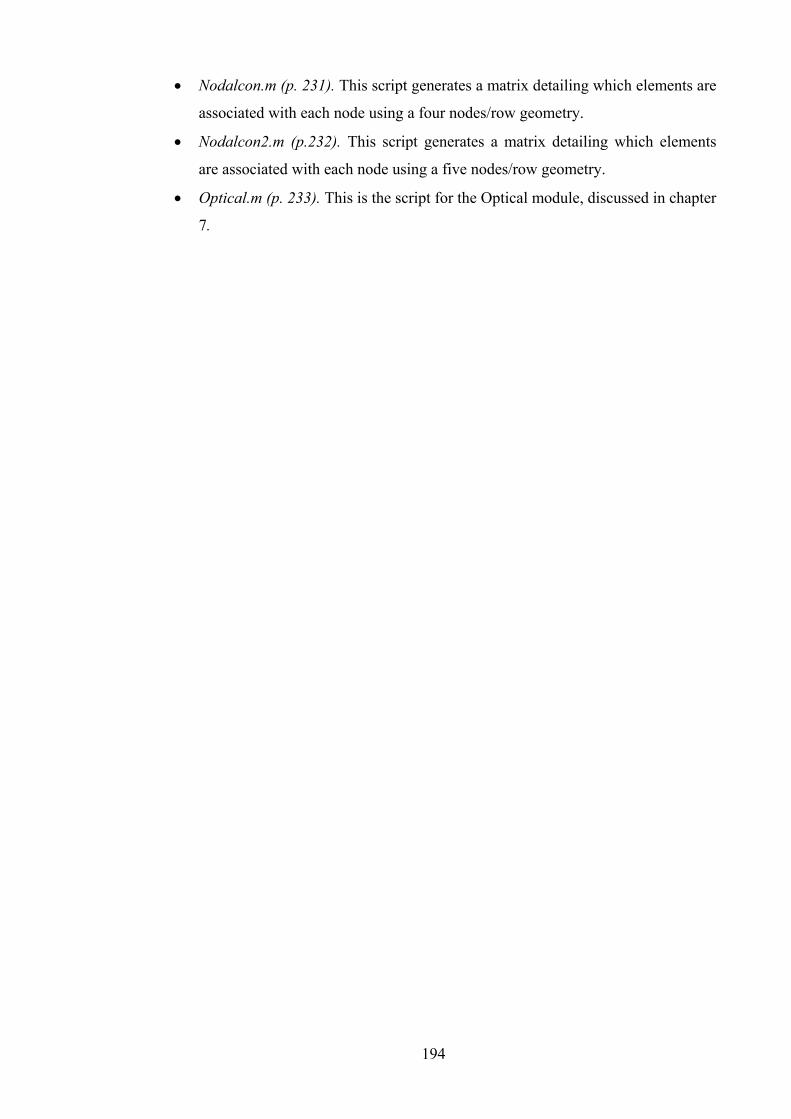
194

• Nodalcon.m (p. 231). This script generates a matrix detailing which elements are

associated with each node using a four nodes/row geometry.

• Nodalcon2.m (p.232). This script generates a matrix detailing which elements

are associated with each node using a five nodes/row geometry.

• Optical.m (p. 233). This is the script for the Optical module, discussed in chapter

7.

196

Chemmod.m code listing

function[fsol1,fsol2,fsol3,sdof] = chemmod(row,col,solvent_level,D,U,F,R,T,z,deltt,flg_gel_elem,flg_gel_node,flg_sol_elem,flg_sol_node,fsol1,fsol2,fsol3,nel,nnel,nnode,EF_sol,EF_gel) %---------------------------------------------------------- % Purpose: Chemical module - solves mass transport equations for each ion in system % % Last modified : 15/04/2005 %----------------------------------------------------------- ndof=1; % number of dofs per node sdof=nnode*ndof; % total system dofs edof=nnel*ndof; % degrees of freedom per element sol_x1 = 1; sol_x2 = col; % solvent boundaries sol_y1 = 1; sol_y2 = solvent_level; % solvent boundaries gel_x1 = 2; gel_x2 = col-1; % gel boundaries gel_y1 = 2; gel_y2 = row; % gel boundaries sol_nodes = size(flg_sol_node,2); sol_elem = size(flg_sol_elem,2); gel_nodes = size(flg_gel_node,2); gel_elem = size(flg_gel_elem,2); %--------------------------------------------------------------------------------------- % Global coordinate values : gcoord(i,j) where i->node no. and j->x or y %--------------------------------------------------------------------------------------- gcoord = globecord(nnode,col); %--------------------------------------------------------------------------------------- % Nodal connectivity for each element : nodes(i,j) where i-> element no. and j-> connected nodes %--------------------------------------------------------------------------------------- nodes = nodalcon(nel,col); %--------------------------------------------------------------------------------------- % 1) Solvent calculations %--------------------------------------------------------------------------------------- %%%%%%%%%% Initialization of matrices and vectors %%%%%%%%%% kk1a=zeros(sol_nodes,sol_nodes); % system matrix - first part kk2a=zeros(sol_nodes,sol_nodes); kk3a=zeros(sol_nodes,sol_nodes); kk1b=zeros(sol_nodes,sol_nodes); % system matrix - second part kk2b=zeros(sol_nodes,sol_nodes); kk3b=zeros(sol_nodes,sol_nodes); kk1=zeros(sol_nodes,sol_nodes); % system matrix - overall kk2=zeros(sol_nodes,sol_nodes); kk3=zeros(sol_nodes,sol_nodes); mm1=zeros(sol_nodes,sol_nodes); % system mass matrix mm2=zeros(sol_nodes,sol_nodes); mm3=zeros(sol_nodes,sol_nodes); %%%%%%%%%% Assemble required matrices from system vectors %%%%%%%%%% for i=1:sol_nodes fsol1s(i,1) = fsol1(flg_sol_node(i)); % copy from system solution vector fsol2s(i,1) = fsol2(flg_sol_node(i)); % copy from system solution vector fsol3s(i,1) = fsol3(flg_sol_node(i)); % copy from system solution vector end; row_count = 1; for i=1:(sol_y2 - sol_y1 + 1) for j=1:(sol_x2 - sol_x1 + 1) soln1(i,j) = fsol1s(row_count); % expand vector into matrix, so as to accurately represent x- and y-derivatives soln2(i,j) = fsol2s(row_count); soln3(i,j) = fsol3s(row_count);

197

row_count = row_count + 1; end; end; %%%%%%%%%% Potential difference %%%%%%%%%% conduct = sum([z(1)^2*U(1)*sum(fsol1s);z(2)^2*U(2)*sum(fsol2s);z(3)^2*U(3)*sum(fsol3s)]); [DX1 DY1] = gradient(soln1); [DX2 DY2] = gradient(soln2); [DX3 DY3] = gradient(soln3); row_count = 1; for i=1:(sol_y2 - sol_y1+1) for j=1:(sol_x2 - sol_x1+1) dC1(row_count) = DX1(i,j) + DY1(i,j); %concentration gradient for 1st species dC2(row_count) = DX2(i,j) + DY2(i,j); dC3(row_count) = DX3(i,j) + DY3(i,j); row_count = row_count + 1; end; end; phi_sol = -(R*T/F) * (sum([ z(1)*U(1)*dC1 ; z(2)*U(2)*dC2 ; z(3)*U(3)*dC3]) / conduct); phi_sol = phi_sol - EF_sol; %%%%%%%%%% Assembly of element matrices %%%%%%%%%% for iel=1:sol_elem % loop for the total number of elements nd(1)=nodes(flg_sol_elem(iel),1); % 1st connected node for (iel)-th element nd(2)=nodes(flg_sol_elem(iel),2); % 2nd connected node for (iel)-th element nd(3)=nodes(flg_sol_elem(iel),3); % 3rd connected node for (iel)-th elemen x1=gcoord(nd(1),1); y1=gcoord(nd(1),2);% coord values of 1st node x2=gcoord(nd(2),1); y2=gcoord(nd(2),2);% coord values of 2nd node x3=gcoord(nd(3),1); y3=gcoord(nd(3),2);% coord values of 3rd node nodes_sol = nodalcon(sol_elem,sol_x2-sol_x1+1); nd(1)=nodes_sol(iel,1); % 1st connected node for (iel)-th element nd(2)=nodes_sol(iel,2); % 2nd connected node for (iel)-th element nd(3)=nodes_sol(iel,3); % 3rd connected node for (iel)-th element index=feeldof(nd,nnel,ndof); % extract system dofs associated with element k1a = D(1) * felp2dt3(x1,y1,x2,y2,x3,y3); % compute element matrix k1b = (U(1)*z(1)/abs(z(1))) * felp2dt3b(x1,y1,x2,y2,x3,y3); % assemble element matrices - part II m1 = felpt2t3(x1,y1,x2,y2,x3,y3); % compute element matrix] k2a = D(2) * felp2dt3(x1,y1,x2,y2,x3,y3); % compute element matrix k2b = (U(2)*z(2)/abs(z(2))) * felp2dt3b(x1,y1,x2,y2,x3,y3); % assemble element matrices - part II m2 = felpt2t3(x1,y1,x2,y2,x3,y3); % compute element matrix] k3a = D(3) * felp2dt3(x1,y1,x2,y2,x3,y3); % compute element matrix k3b = (U(3)*z(3)/abs(z(3))) * felp2dt3b(x1,y1,x2,y2,x3,y3); % assemble element matrices - part II m3 = felpt2t3(x1,y1,x2,y2,x3,y3); % compute element matrix] kk1a=feasmbl1(kk1a,k1a,index); % assemble element matrices kk1b=feasmbl1(kk1b,k1b,index); mm1= feasmbl1(mm1,m1,index); % assemble element matrices kk2a=feasmbl1(kk2a,k2a,index); % assemble element matrices kk2b=feasmbl1(kk2b,k2b,index); mm2= feasmbl1(mm2,m2,index); % assemble element matrices kk3a=feasmbl1(kk2a,k3a,index); % assemble element matrices kk3b=feasmbl1(kk2b,k3b,index); mm3= feasmbl1(mm2,m3,index); % assemble element matrices end; for i = 1:size(fsol1s,1) kk1b(:,i) = kk1b(:,i) * phi_sol(i); kk2b(:,i) = kk2b(:,i) * phi_sol(i); kk3b(:,i) = kk3b(:,i) * phi_sol(i); end; kk1 = kk1a + kk1b; kk2 = kk2a + kk2b; kk3 = kk3a + kk3b;

198

%%%%%%%%%% Calculations %%%%%%%%%% fsol1s = (mm1 + deltt*kk1) \ (mm1 * fsol1s); fsol2s = (mm2 + deltt*kk2) \ (mm2 * fsol2s); fsol1s = (mm3 + deltt*kk3) \ (mm3 * fsol3s); %%%%%%%%%% Recombination %%%%%%%%%% for i=1:sol_nodes fsol1(flg_sol_node(i)) = fsol1s(i); % copy from system solution vector fsol2(flg_sol_node(i)) = fsol2s(i); fsol3(flg_sol_node(i)) = fsol3s(i); end; %--------------------------------------------------------------------------------------- % 2) Gel calculations %--------------------------------------------------------------------------------------- clear soln1 soln2 soln3 kk1a kk2a kk3a kk1b kk2b kk3b mm1 mm2 mm3; %%%%%%%%%% Initialization of matrices and vectors %%%%%%%%%% kk1a=zeros(gel_nodes,gel_nodes); % system matrix - first part kk2a=zeros(gel_nodes,gel_nodes); kk3a=zeros(gel_nodes,gel_nodes); kk1b=zeros(gel_nodes,gel_nodes); % system matrix - second part kk2b=zeros(gel_nodes,gel_nodes); kk3b=zeros(gel_nodes,gel_nodes); kk1=zeros(gel_nodes,gel_nodes); % system matrix - overall kk2=zeros(gel_nodes,gel_nodes); kk3=zeros(gel_nodes,gel_nodes); mm1=zeros(gel_nodes,gel_nodes); % system mass matrix mm2=zeros(gel_nodes,gel_nodes); mm3=zeros(gel_nodes,gel_nodes); %%%%%%%%%% Assemble required matrices from system vectors %%%%%%%%%% for i=1:gel_nodes fsol1g(i,1) = fsol1(flg_gel_node(i)); % copy from system solution vector fsol2g(i,1) = fsol2(flg_gel_node(i)); % copy from system solution vector fsol3g(i,1) = fsol3(flg_gel_node(i)); % copy from system solution vector end; row_count = 1; for i=1:(gel_y2 - gel_y1 + 1) for j=1:(gel_x2 - gel_x1 + 1) soln1(i,j) = fsol1g(row_count); % expand vector into matrix, so as to accurately represent x- and y-derivatives soln2(i,j) = fsol2g(row_count); soln3(i,j) = fsol3g(row_count); row_count = row_count + 1; end; end; %%%%%%%%%% Potential difference %%%%%%%%%% conduct = sum([z(1)^2*U(1)*sum(fsol1g);z(2)^2*U(2)*sum(fsol2g);z(3)^2*U(3)*sum(fsol3g)]); [DX1 DY1] = gradient(soln1); [DX2 DY2] = gradient(soln2); [DX3 DY3] = gradient(soln3); row_count = 1; for i=1:(gel_y2 - gel_y1+1) for j=1:(gel_x2 - gel_x1+1) dC1(row_count) = DX1(i,j) + DY1(i,j); dC2(row_count) = DX2(i,j) + DY2(i,j); dC3(row_count) = DX3(i,j) + DY3(i,j); row_count = row_count + 1; end; end; phi_gel = -(R*T/F) * (sum([ z(1)*U(1)*dC1 ; z(2)*U(2)*dC2 ; z(3)*U(3)*dC3]) / conduct); phi_gel = phi_gel - EF_gel; %%%%%%%%%% Assembly of element matrices %%%%%%%%%%

199

for iel=1:gel_elem % loop for the total number of elements nd(1)=nodes(flg_gel_elem(iel),1); % 1st connected node for (iel)-th element nd(2)=nodes(flg_gel_elem(iel),2); % 2nd connected node for (iel)-th element nd(3)=nodes(flg_gel_elem(iel),3); % 3rd connected node for (iel)-th elemen x1=gcoord(nd(1),1); y1=gcoord(nd(1),2);% coord values of 1st node x2=gcoord(nd(2),1); y2=gcoord(nd(2),2);% coord values of 2nd node x3=gcoord(nd(3),1); y3=gcoord(nd(3),2);% coord values of 3rd node nodes_gel = nodalcon(gel_elem,gel_x2-gel_x1+1); nd(1)=nodes_gel(iel,1); % 1st connected node for (iel)-th element nd(2)=nodes_gel(iel,2); % 2nd connected node for (iel)-th element nd(3)=nodes_gel(iel,3); % 3rd connected node for (iel)-th element index=feeldof(nd,nnel,ndof);% extract system dofs associated with element k1a = D(1) * felp2dt3(x1,y1,x2,y2,x3,y3); % compute element matrix k1b = (U(1)*z(1)/abs(z(1))) * felp2dt3b(x1,y1,x2,y2,x3,y3); % assemble element matrices - part II m1 = felpt2t3(x1,y1,x2,y2,x3,y3); % compute element matrix] k2a = D(2) * felp2dt3(x1,y1,x2,y2,x3,y3); % compute element matrix k2b = (U(2)*z(2)/abs(z(2))) * felp2dt3b(x1,y1,x2,y2,x3,y3); % assemble element matrices - part II m2 = felpt2t3(x1,y1,x2,y2,x3,y3); % compute element matrix] k3a = D(3) * felp2dt3(x1,y1,x2,y2,x3,y3); % compute element matrix k3b = (U(3)*z(3)/abs(z(3))) * felp2dt3b(x1,y1,x2,y2,x3,y3); % assemble element matrices - part II m3 = felpt2t3(x1,y1,x2,y2,x3,y3); % compute element matrix] kk1a=feasmbl1(kk1a,k1a,index); % assemble element matrices kk1b=feasmbl1(kk1b,k1b,index); mm1= feasmbl1(mm1,m1,index); % assemble element matrices kk2a=feasmbl1(kk2a,k2a,index); % assemble element matrices kk2b=feasmbl1(kk2b,k2b,index); mm2= feasmbl1(mm2,m2,index); % assemble element matrices kk3a=feasmbl1(kk2a,k3a,index); % assemble element matrices kk3b=feasmbl1(kk2b,k3b,index); mm3= feasmbl1(mm2,m3,index); % assemble element matrices end; for i = 1:size(fsol1g,1) kk1b(:,i) = kk1b(:,i) * phi_gel(i); kk2b(:,i) = kk2b(:,i) * phi_gel(i); kk3b(:,i) = kk3b(:,i) * phi_gel(i); end; kk1 = kk1a + kk1b; kk2 = kk2a + kk2b; kk3 = kk3a + kk3b; %%%%%%%%%% Calculations %%%%%%%%%% fsol1g = (mm1 + deltt*kk1) \ (mm1 * fsol1g); fsol2g = (mm2 + deltt*kk2) \ (mm2 * fsol2g); fsol3g = (mm3 + deltt*kk3) \ (mm3 * fsol3g); %%%%%%%%%% Recombination %%%%%%%%%% for i=1:gel_nodes fsol1(flg_gel_node(i)) = fsol1g(i); % copy from system solution vector fsol2(flg_gel_node(i)) = fsol2g(i); fsol3(flg_gel_node(i)) = fsol3g(i); end;

200

Control.m code listing

%---------------------------------------------------------- % Purpose: Main control program - this is the "front end" for the overall model % All user enterable data is inputted into this file % % Last modified : 11/09/2005 %----------------------------------------------------------- clear; clc; close all; format short g; delete *.*.dat; % deletes any previous data files - may need reviewing later... %---------------------------------------------------------------------------------------% Constants - these shouldn't need adjustment! %--------------------------------------------------------------------------------------- e = 1.602e-19; % elementary charge R = 8.31451; % uiversal gas constant T = 293.15; % Ambient temperature (Kelvin) F = 96485.31; % Faraday constant kb = 1.38066e-23; % Boltzmann epsilon0 = 8.854e-12; % Permittivity of free space epsilonR = 81.07; % Dielectric constant of water CHI = 0.48; % Flory-Huggins Interaction parameter %--------------------------------------------------------------------------------------- % Control parameters %--------------------------------------------------------------------------------------- %%% Geometry %%% x_size = 27; y_size = 7; dim_x = 19e-3; % dimensions of gel in x direction (m) - used to scale nnel=3; % number of nodes per element (triangular) solvent_level = 4; % How much solvent?? Absolute, so add one for measuring from gel base!! %%% Time Control %%% stime = 0; % Start time ftime = 300; % End time deltt = 0.1; % time step for transient analysis ntime = fix((ftime-stime)/deltt); % number of time increments %%% Movie generation %%% makemov = 0; % Generate movie : Options are 0=off, 1=unique filename, 2=set filename to 'swell.avi' p_anim = 1; % Pause before movie generation? 0=off, 1=on frame_grab = 10; % Grab every i-th frame sound_alert = 0; % plays sound when loop finished %%% Electrical parameters %%% Vtop = 0; % voltage at top of gel region Vbot = 7.5; % voltage at bottom of gel region epsilonLJ = 809*kb; % Lennard-Jones potential well depth sigmaLJ = 0.265e-9; % Lennard-Jones molecular separation (in meters - r in gel_distribute must have SAME UNITS!!!) no_ions = 20; % When distributing ions in gel region, this determines into how many parts the ion conc is divided into! %%% Chemical parameters (Na+ = 1; Cl- = 2; OH-stat = 3) %%% sol_conc = 4; % Surrounding NaCL solution concentration - molar volume = 1/sol_conc (m^3/mol) gel_conc = [0.46358; 0; 0.46358]; % (1 = 2+3) D = [1.545e-5 ; 1.545e-5 ; 0]; % diffusion coefficient z = [1 ; -1 ; -1]; % charge numbers Vs = 50; % Amount of water in total system(ml)

201

Vp = 4.8; % Amount of polymer solution in total system (ml) Vb = 5.6; % Amount of additional liquid elements in total system(eg. NaOH) (ml) V_sample = (0.019 * 0.005)*1000; % Volume of sample being used (1 * length * height - converted to litres) (L) %%% Mechanical parameters %%% emodule=0.0547e6; % elastic modulus poisson=0.43; % Poisson's ratio rho = 1.08; % Mass density b=0; % Viscous damping coefficient ral_alpha = 0; % Raleigh alpha damping constant (leave as zero to use lumped damping) ral_beta = 0; % Raleigh alpha damping constant %---------------------------------------------------------------------------------------% Generated parameters (from user-entered Control parameters) %--------------------------------------------------------------------------------------- % Geometrical parameters % col = x_size + 2; row = y_size + 1; nnode = col*row; % total number of nodes in system nel = 2 * (row-1) * (col-1); % number of elements sol_x1 = 1; sol_x2 = col; % solvent boundaries sol_y1 = 1; sol_y2 = solvent_level; % solvent boundaries gel_x1 = 2; gel_x2 = col-1; % gel boundaries gel_y1 = 2; gel_y2 = row; % gel boundaries scale = dim_x / ((col-1) - 2 + 1); % size of each element in gel % Chemical module parameters: Na+ = 1; Cl- = 2; OH- = 3 % soln1 = zeros(row,col); % CHEMICAL system matrices for each component soln2 = zeros(row,col); soln3 = zeros(row,col); U = [D(1)*abs(z(1))*F/(R*T) ; D(2)*abs(z(2))*F/(R*T) ; D(3)*abs(z(3))*F/(R*T)]; % electrolytic mobility Vtot = Vs + Vp + Vb; % Total volume of gel sample (for volume fraction) Vs = (Vs/Vtot) * V_sample; % Amount of solvent in gel sample Vp = (Vp/Vtot) * V_sample; Vb = (Vb/Vtot) * V_sample; Vcell = V_sample/(x_size*y_size); % Total volume of gel sample (Vs+Vp+Vb should add to this!) lambdaB = e^2/(4*pi*epsilon0*epsilonR*kb*T); % Bjerrum Length % Mechanical module parameters - Part 1% displ = zeros(((gel_x2-gel_x1+1)*(gel_y2-gel_y1+1) + ((gel_x2-gel_x1)*(gel_y2-gel_y1)))*2,1); velc = zeros(((gel_x2-gel_x1+1)*(gel_y2-gel_y1+1) + ((gel_x2-gel_x1)*(gel_y2-gel_y1)))*2,1); % Movie generation and post-processing parameters % path_store = cd; cd d:\temp; % path to movie file NAME = sprintf('%d',num2str(now)); NAME = num2str(NAME); appendTofile(sprintf('%s.dat',NAME),displ',';') cd(path_store); %--------------------------------------------------------------------------------------- % Flags - these identify which nodes & elements are associated with the % sol and gel %--------------------------------------------------------------------------------------- [flg_sol_node,flg_sol_elem,flg_gel_node,flg_gel_elem] = flager(row,col,solvent_level); %--------------------------------------------------------------------------------------- % Set up gel and solvent matrices with appropriate concentrations %---------------------------------------------------------------------------------------

202

% Distribute solvent ions % disp('Distributing ions, please wait...') for i=1:solvent_level for j=1:col if i >= 2 & i <= row & j >= 2 & j <= col-1 soln1(i,j) = 0; else soln1(i,j) = sol_conc; end; end end soln2 = soln1; % Distribute gel region ions % % This code can be executed prior, and then loaded directly - gel_distribute is quite memory intensive, and this can save time! % [S1,S3] = gel_distribute(row,col,scale,kb,T,lambdaB,epsilonLJ,sigmaLJ,z(1),z(2),gel_conc(1),no_ions); % Uncomment to generate new ion concentration is hydrogel region S1 = dlmread('S1data.dat','\t'); % write data using dlmwrite('S1data.dat',S1,'\t') after using gel_distribute; S3 = dlmread('S3data.dat','\t'); % write data using dlmwrite('S3data.dat',S3,'\t') after using gel_distribute; row_count = 1; for i=gel_y1:gel_y2 for j=gel_x1:gel_x2 soln1(i,j) = S1(row_count); soln3(i,j) = S3(row_count); row_count = row_count + 1; end; end; % Wrap matrices back into vectors % row_count = 1; for i=1:row for j=1:col fsol1(row_count) = soln1(i,j); % wrap the matrix back into a vector (so that is can be multiplied etc). fsol2(row_count) = soln2(i,j); fsol3(row_count) = soln3(i,j); row_count = row_count + 1; end; end; fsol1 = fsol1'; fsol2 = fsol2'; fsol3 = fsol3'; cell_vols = (ones(size(flg_gel_node,2),1)) * Vcell; % Initial volume of cell (based on size of gel sample and number of elements) %---------------------------------------------------------------------------------------% Set up nodes and coordinates for Mechanical module - this must be done % here, or the program gets upset!! %--------------------------------------------------------------------------------------- gcoord = globecord2(((gel_x2-gel_x1+1)*(gel_y2-gel_y1+1))+(gel_x2-gel_x1)*(gel_y2-gel_y1),(gel_x2-gel_x1+1)); gnel = size(flg_gel_elem,2)*2; gnodes = nodalcon2(gnel,(gel_x2-gel_x1+1)); gsdof = (((gel_x2-gel_x1+1)*(gel_y2-gel_y1+1))+(gel_x2-gel_x1)*(gel_y2-gel_y1)) * 2; gedof = nnel * 2; %--------------------------------------------------------------------------------------- % External electric field %--------------------------------------------------------------------------------------- EF = efield2(Vtop,Vbot,col,row,solvent_level); [px py] = gradient(EF,(dim_x / col)); px = px * -1; py = py * -1; G = px+py;

203

G = G/1000 % scaling factor! Needed to ensure stability of Chemical module! :-( % Wrap E-field matrix into vectors row_count = 1; for i=1:row for j=1:col if i <= sol_y2 EF_sol(row_count) = G(i,j); row_count = row_count + 1; end end; end; row_count = 1; for i=gel_y1:gel_y2 for j=gel_x1:gel_x2 EF_gel(row_count) = G(i,j); row_count = row_count + 1; end; end; %--------------------------------------------------------------------------------------- % loop for time integration %--------------------------------------------------------------------------------------- for it=1:ntime if mod(it,100) == 0 disp('PAUSE - abort NOW if required'); pause(1); % brief pause to enable you to abort if neccessary! end clk = clock; progr = sprintf('Processing... %1.2f%% complete [%d.%d.%.0f]',(it/ntime*100),clk(4),clk(5),clk(6)) progr = num2str(progr); % Write data to file - for remote monitoring % cd H:\data\DEM_reports; delete *.*; dlmwrite(sprintf('%s',progr),0) cd(path_store); % Restore original concentrations row_count = 1; for i=1:row for j=1:col if soln2(i,j) ~= 0 fsol1(row_count) = soln1(i,j); fsol2(row_count) = soln2(i,j); end row_count = row_count + 1; end; end; row_count = 1; for i=1:row for j=1:col fsol3(row_count) = soln3(i,j); row_count = row_count + 1; end; end; %----------------------------------------------------------------------------------- % Chemical module %----------------------------------------------------------------------------------- [fsol1_new,fsol2_new,fsol3_new,sdof] = chemmod(row,col,solvent_level,D,U,F,R,T,z,deltt,flg_gel_elem,flg_gel_node,flg_sol_elem,flg_sol_node,fsol1,fsol2,fsol3,nel,nnel,nnode,EF_sol,EF_gel); %----------------------------------------------------------------------------------- % Bridging equations (converted chemical --> forces) %-----------------------------------------------------------------------------------

204

[ff,cell_vols] = forcer(fsol1_new,fsol2_new,fsol3_new,fsol1,fsol2,fsol3,cell_vols,sdof,row,col,solvent_level,flg_gel_node,CHI,Vp,sol_conc,Vtot,R,T,dim_x); [ff] = force_changer(ff,(col-1)-2,row-2); % tranlates the forces from 2 elements/row triangles to 4 element/row forces(:,it) = ff; %----------------------------------------------------------------------------------- % Mechanical module %----------------------------------------------------------------------------------- [displ,velc] = mech(deltt,emodule,poisson,rho,b,ral_alpha,ral_beta,gcoord,gnodes,(gel_x2-gel_x1+1),nnel,gnel,gsdof,gedof,2,ff,displ,velc); %----------------------------------------------------------------------------------- % Restore solution vectors fsol_new --> fsol %----------------------------------------------------------------------------------- fsol1 = fsol1_new; fsol2 = fsol2_new; fsol3 = fsol3_new; %----------------------------------------------------------------------------------- % Store displacement data %----------------------------------------------------------------------------------- cd d:\temp; appendTofile(sprintf('%s.dat',NAME),displ',';') cd(path_store); end; %%% END OF TIME LOOP %--------------------------------------------------------------------------------------- % Post processing %--------------------------------------------------------------------------------------- if makemov == 1 if p_anim == 1 clc disp('Press any key to begin post-processing visualisation') pause; end; draw(gcoord,(gel_x2-gel_x1),(gel_y2-gel_y1),gnodes,gnel,deltt,frame_grab,ntime,NAME,makemov) cd(path_store); end

Draw.m code listing

function draw(gcoord,col,row,gnodes,gnel,deltt,frame_grab,ntime,NAME,makemov) %---------------------------------------------------------- % Purpose: Drawing module - this calculates the post-visulisation sequences used for this work % % Last modified : 21/06/2005 %----------------------------------------------------------- format short g; % Movie generation / data storage parameters % if makemov == 1 cd d:\temp; aviobj = avifile(sprintf('%s.avi',NAME),'fps',1,'compression','Indeo3','quality',100); end; if makemov == 2 cd d:\temp; aviobj = avifile('swell.avi','fps',1,'compression','Indeo3','quality',100); end; % Plot initial coordinates gcoord(:,1) = gcoord(:,1) - (col/2); gcoord(:,2) = gcoord(:,2) - (row/2);

205

for it=1:ntime % Read displacement data if mod(it,frame_grab) == 0 & it ~= 1 % Output progress report to file - useful for remote monitoring clk = clock; progr = sprintf('Plotting... %1.2f%% complete [%d.%d.%.0f]',(it/ntime*100),clk(4),clk(5),clk(6)); progr = num2str(progr); cd H:\data\DEM_reports; delete *.*; dlmwrite(sprintf('%s',progr),0) cd d:\temp; displ = dlmread(sprintf('%s.dat',NAME),';'); % make large vector!! displ = (displ(it,:))'; sdof = size(displ,1); %%% Initial nodal positions %%% figure(1); clf; scatter(gcoord(:,1),gcoord(:,2),'yo'); axis([min(gcoord(:,1))-1 max(gcoord(:,1))+1 min(gcoord(:,2))-1 max(gcoord(:,2))+1]); % Fitted to size axes hold on; current_disp_x = gcoord(:,1) + displ(1:2:sdof); current_disp_y = gcoord(:,2) + displ(2:2:sdof); scatter(current_disp_x,current_disp_y,'ko'); for i=1:gnel for j=1:3 x(j)=current_disp_x(gnodes(i,j)); y(j)=current_disp_y(gnodes(i,j)); end; xvec = [x(1),x(2),x(3),x(1)]; %. Draw element boundaries yvec = [y(1),y(2),y(3),y(1)]; plot(xvec,yvec,'k-'); end; text(min(gcoord(:,1)),max(gcoord(:,2)+0.75),sprintf('Time = %1.2f',it*deltt)); drawnow; if makemov ~= 0 frame = getframe(gca); aviobj = addframe(aviobj,frame); end; end; end; if makemov ~= 0 aviobj = close(aviobj); end; close all;

206

Efield1.m code listing

function V2 = efield(gel_x2,gel_x1,gel_y2,gel_y1,sol_y2,Vtop,Vbot,row,col) %---------------------------------------------------------------------------- % Program to generate E-field - Type 1 % Last modifed : 28/10/04 % Second version - major modifications to program % This is being built to allow a 1-to-1 correlation in the rest of the % model - this is why the solvent is shown, although at constant voltage, % so those elements will form a zero E-field... % % This version assumes that there is no solvent (and thus no e-field) below % the gel %---------------------------------------------------------------------------- solvent_level = sol_y2-gel_y1; solvent_col = 3; gel_x = gel_x2 - gel_x1 + 1; gel_y = gel_y2 - gel_y1 + 1; V2 = zeros(row,col); %%%%%%%%%%%% form matrices and vectors %%%%%%%%%%%%%% gel_half = ceil(gel_x/2); % This is the one that actually counts! gel_half2 = gel_half - solvent_col rc = 1; % matrix counter V = zeros(gel_y,gel_half) + inf; V(1,gel_half) = Vtop; V2 = zeros(gel_y,gel_x); V3 = zeros(gel_y,gel_x); for i=1:gel_y-solvent_level-1 for j=1:solvent_col V(i,j) = 0; end end for i=gel_y-solvent_level:gel_y for j=1:solvent_col V(i,j) = Vbot; end end; voltage = zeros(size(find(V==inf),1)); %%%%%%%%%%%% assemble vectors %%%%%%%%%%%%%% for i=1:size(V,1) %row for j=1:size(V,2) %col if V(i,j) == inf if j == solvent_col + 1 % first column of gel if i == 1 % first row voltage(rc,rc) = 2; voltage(rc,rc+1) = -1; voltage(rc,rc+(gel_half2-1)) = -1; voltage2(rc) = 0; elseif i == 2 % second row voltage(rc,rc) = 3; voltage(rc,rc+1) = -1; voltage(rc,rc+gel_half2) = -1; voltage(rc,rc-(gel_half2-1)) = -1; voltage2(rc) = 0; elseif i >= (gel_y - solvent_level) & i~=gel_y % solvent rows voltage(rc,rc) = 4; voltage(rc,rc+1) = -1; voltage(rc,rc-gel_half2) = -1; voltage(rc,rc+gel_half2) = -1; voltage2(rc) = Vbot; elseif i == gel_y % last row

207

voltage(rc,rc) = 3; voltage(rc,rc+1) = -1; voltage(rc,rc-gel_half2) = -1; voltage2(rc) = Vbot; else voltage(rc,rc) = 3; voltage(rc,rc+1) = -1; voltage(rc,rc-gel_half2) = -1; voltage(rc,rc+gel_half2) = -1; voltage2(rc) = 0; end; rc = rc + 1; elseif j == (solvent_col + 2) & j ~= (gel_half -1) % true j = 2 (ie. not row before centre) if i == 1 % first row voltage(rc,rc) = 3; voltage(rc,rc-1) = -1; voltage(rc,rc+1) = -1; voltage(rc,rc+(gel_half2-1)) = -1; voltage2(rc) = 0; elseif i == 2 % second row voltage(rc,rc) = 4; voltage(rc,rc-1) = -1; voltage(rc,rc+1) = -1; voltage(rc,rc-(gel_half2-1)) = -1; voltage(rc,rc+gel_half2) = -1; voltage2(rc) = 0; elseif i == gel_y % last row voltage(rc,rc) = 3; voltage(rc,rc+1) = -1; voltage(rc,rc-1) = -1; voltage(rc,rc-gel_half2) = -1; voltage2(rc) = 0; else voltage(rc,rc) = 4; voltage(rc,rc+1) = -1; voltage(rc,rc-1) = -1; voltage(rc,rc-gel_half2) = -1; voltage(rc,rc+gel_half2) = -1; voltage2(rc) = 0; end; rc = rc + 1; elseif j == gel_half-1 & j ~= (solvent_col + 2) % true next to centre column if i == 1 voltage(rc,rc) = 3; voltage(rc,rc-1) = -1; voltage(rc,rc+(gel_half2-1)) = -1; voltage2(rc) = Vtop; elseif i == 2 voltage(rc,rc) = 4; voltage(rc,rc+1) = -1; voltage(rc,rc-1) = -1; voltage(rc,rc-(gel_half2-1)) = -1; voltage(rc,rc+gel_half2) = -1; voltage2(rc) = 0; elseif i == gel_y voltage(rc,rc) = 3; voltage(rc,rc-1) = -1; voltage(rc,rc+1) = -1; voltage(rc,rc-gel_half2) = -1; voltage2(rc) = 0; else voltage(rc,rc) = 4; voltage(rc,rc-1) = -1; voltage(rc,rc+1) = -1; voltage(rc,rc-gel_half2) = -1; voltage(rc,rc+gel_half2) = -1; voltage2(rc) = 0; end; rc = rc + 1; elseif j == gel_half-1 & j == (solvent_col + 2) % dual case (ie. both second col and 2nd last col) if i == 1 voltage(rc,rc) = 3; voltage(rc,rc-1) = -1; voltage(rc,rc+(gel_half2-1)) = -1;

208

voltage2(rc) = Vtop; elseif i == 2 voltage(rc,rc) = 4; voltage(rc,rc+1) = -1; voltage(rc,rc-1) = -1; voltage(rc,rc-(gel_half2-1)) = -1; voltage(rc,rc+gel_half2) = -1; voltage2(rc) = 0; elseif i == gel_y voltage(rc,rc) = 3; voltage(rc,rc+1) = -1; voltage(rc,rc-gel_half2) = -1; voltage2(rc) = 0; else voltage(rc,rc) = 4; voltage(rc,rc-1) = -1; voltage(rc,rc+1) = -1; voltage(rc,rc-gel_half2) = -1; voltage(rc,rc+gel_half2) = -1; voltage2(rc) = 0; end; rc = rc + 1; elseif j == gel_half % centre column if i == 2 voltage(rc,rc) = 4; voltage(rc,rc-1) = -2; voltage(rc,rc+gel_half2) = -1; voltage2(rc) = Vtop; elseif i == gel_y voltage(rc,rc) = 3; voltage(rc,rc-1) = -2; voltage(rc,rc-gel_half2) = -1; voltage2(rc) = 0; else voltage(rc,rc) = 4; voltage(rc,rc-1) = -2; voltage(rc,rc+gel_half2) = -1; voltage(rc,rc-gel_half2) = -1; voltage2(rc) = 0; end; rc = rc + 1; else if i == 1 voltage(rc,rc) = 3; voltage(rc,rc-1) = -1; voltage(rc,rc+1) = -1; voltage(rc,rc+(gel_half2-1)) = -1; voltage2(rc) = 0; elseif i == 2 voltage(rc,rc) = 4; voltage(rc,rc-1) = -1; voltage(rc,rc+1) = -1; voltage(rc,rc-(gel_half2-1)) = -1; voltage(rc,rc+gel_half2) = -1; voltage2(rc) = 0; elseif i == gel_y voltage(rc,rc) = 3; voltage(rc,rc-1) = -1; voltage(rc,rc+1) = -1; voltage(rc,rc-gel_half2) = -1; voltage2(rc) = 0; else voltage(rc,rc) = 4; voltage(rc,rc-1) = -1; voltage(rc,rc+1) = -1; voltage(rc,rc-gel_half2) = -1; voltage(rc,rc+gel_half2) = -1; voltage2(rc) = 0; end; rc = rc + 1; end end; % end of infinity loop end; % end of j loop end; % end of i loop

209

%%%%%%%%%%%% calculations %%%%%%%%%%%%%% voltage2 = voltage2'; voltage3 = voltage\voltage2; %%%%%%%%%%%% reassemble matrices %%%%%%%%%%%%%% rc = 1; for i=1:size(V,1) %row for j=1:size(V,2) %col if V(i,j) == inf V(i,j) = voltage3(rc); rc = rc + 1; end; end; end; %%%%%%%%%%%% mirror matrix %%%%%%%%%%%%%% for i=1:size(V,1) %row rc = 0; for j=1:(gel_half-1) V(i,(gel_x-rc)) = V(i,j); rc = rc+1; end; end; %%%%%%%%%% turn matrix upside down... %%%%%%%%%%%%%% rc = 1; for i=size(V,1):-1:1 V2(rc,:) = V(i,:); rc = rc + 1; end; %%%%%%%%%%% plot contours & quivers %%%%%%%%%%%%% [c,h] = contour(V2); clabel(c,h); axis equal; axis auto; hold on; x = [1 1 gel_x gel_x 1]; y = [1 gel_y gel_y 1 1]; anode_x = [gel_half gel_half]; anode_y = [gel_y gel_y+1]; cath_x = [1 1 gel_x gel_x]; cath_y = [solvent_level+1 1 1 solvent_level+1]; [px,py] = gradient(V2); px = px * -1; % correction factor - because quiver plots point from py = py * -1; % the lowest point to the highest (ie. the % opposite to the E-field quiver(px,py); V2 px+py %%%%% Reforming into a matrix %%%%%%%%%%% T = reshape(V',gel_x*gel_y,1); rc = 1; for i=1:row for j=1:col if i > row-sol_y2 V2(i,j) = Vbot; end if i <= row - gel_y1 + 1 if j >= gel_x1 & j <= gel_x2 V2(i,j) = T(rc); rc = rc + 1; end end end end V2;

210

[px,py] = gradient(V2); px = abs(px); py = abs(py); GR = px + py;


function V2 = efield2(Vtop,Vbot,gel_x,gel_y,solvent_level) %---------------------------------------------------------------------------- % Program to generate E-field - Type 2 % Last modifed : 13/06/05 % Second version - major modifications to program % This is being built to allow a 1-to-1 correlation in the rest of the % model - this is why the solvent is shown, although at constant voltage, % so those elements will form a zero E-field... % % This version assumes that there is a solvent (and thus an e-field) below % the gel %---------------------------------------------------------------------------- %%%%%%%%%%%% Checks for a properly formed matrix %%%%%%%%%%%%%% if mod(gel_x,2) == 0 clc disp('********************************************************************') disp('*** ERROR : E solver needs an odd number of nodes in x-direction ***'); disp('********************************************************************') pause; end; if (gel_y-solvent_level-1) <=2 clc disp('*************************************************************************') disp('*** Solvent level is too high for model! Set lower and re-run program ***'); disp('*************************************************************************') pause; end; %%%%%%%%%%%% Form matrices and vectors %%%%%%%%%%%%%% gel_half = ceil(gel_x/2); % This is the one that actually counts! rc = 1; % matrix counter V = zeros(gel_y,gel_half) + inf; V2 = zeros(gel_y,gel_x); for i=gel_y-(solvent_level-1):gel_y V(i,1) = Vbot; end V(gel_y,:) = Vbot; voltage = zeros(size(find(V==inf),1)); %%%%%%%%%%%% assemble vectors %%%%%%%%%%%%%% for i=1:size(V,1) %row for j=1:size(V,2) %col if V(i,j) == inf if j == 1 % first column of system if i==1 voltage(rc,rc) = 2; voltage(rc,rc+1) = -1; voltage(rc,rc+gel_half) = -1; voltage2(rc) = 0; elseif i == 2 voltage(rc,rc) = 3; voltage(rc,rc+1) = -1; voltage(rc,rc-gel_half) = -1; voltage(rc,rc+gel_half) = -1; voltage2(rc) = 0; elseif i == (gel_y - solvent_level) % level above solvent voltage(rc,rc) = 3;

211

voltage(rc,rc+1) = -1; voltage(rc,rc-gel_half) = -1; voltage2(rc) = Vbot; else voltage(rc,rc) = 3; voltage(rc,rc+1) = -1; voltage(rc,rc-gel_half) = -1; voltage(rc,rc+gel_half) = -1; voltage2(rc) = 0; end rc = rc + 1; elseif j == 2 % first column of gel if i == 1 voltage(rc,rc) = 2; voltage(rc,rc+1) = -1; voltage(rc,rc+gel_half) = -1; voltage2(rc) = 0; elseif i == 2 voltage(rc,rc) = 3; voltage(rc,rc+1) = -1; voltage(rc,rc-gel_half) = -1; voltage(rc,rc+gel_half) = -1; voltage2(rc) = 0; elseif i == (gel_y - solvent_level) voltage(rc,rc) = 3; voltage(rc,rc+1) = -1; voltage(rc,rc-gel_half) = -1; voltage(rc,rc+(gel_half-1)) = -1; voltage2(rc) = 0; elseif i > (gel_y - solvent_level) & i~=gel_y-1 % solvent rows voltage(rc,rc) = 4; voltage(rc,rc+1) = -1; voltage(rc,rc-(gel_half-1)) = -1; voltage(rc,rc+(gel_half-1)) = -1; voltage2(rc) = Vbot; elseif i == (gel_y-1) % last row voltage(rc,rc) = 4; voltage(rc,rc+1) = -1; voltage(rc,rc-(gel_half-1)) = -1; voltage2(rc) = 2*Vbot; else voltage(rc,rc) = 3; voltage(rc,rc+1) = -1; voltage(rc,rc-gel_half) = -1; voltage(rc,rc+gel_half) = -1; voltage2(rc) = 0; end; rc = rc + 1; elseif j == gel_half-1 % next to centre column if i == 1 voltage(rc,rc) = 3; voltage(rc,rc-1) = -1; voltage(rc,rc+gel_half) = -1; voltage2(rc) = Vtop; elseif i == 2 voltage(rc,rc) = 4; voltage(rc,rc-1) = -1; voltage(rc,rc+1) = -1; voltage(rc,rc-gel_half) = -1; voltage(rc,rc+gel_half) = -1; voltage2(rc) = 0; elseif i == gel_y - solvent_level voltage(rc,rc) = 4; voltage(rc,rc-1) = -1; voltage(rc,rc+1) = -1; voltage(rc,rc-gel_half) = -1; voltage(rc,rc+(gel_half-1)) = -1; voltage2(rc) = 0; elseif i > (gel_y - solvent_level) & i~=gel_y-1 voltage(rc,rc) = 4; voltage(rc,rc-1) = -1; voltage(rc,rc+1) = -1; voltage(rc,rc-(gel_half-1)) = -1; voltage(rc,rc+(gel_half-1)) = -1; voltage2(rc) = 0;

212

elseif i == gel_y-1 voltage(rc,rc) = 4; voltage(rc,rc-1) = -1; voltage(rc,rc+1) = -1; voltage(rc,rc-(gel_half-1)) = -1; voltage2(rc) = Vbot; else voltage(rc,rc) = 4; voltage(rc,rc-1) = -1; voltage(rc,rc+1) = -1; voltage(rc,rc-gel_half) = -1; voltage(rc,rc+gel_half) = -1; voltage2(rc) = 0; end; rc = rc + 1; elseif j == gel_half % centre column if i == 1 voltage(rc,rc) = 1; voltage2(rc) = Vtop; elseif i == 2 voltage(rc,rc) = 4; voltage(rc,rc-1) = -2; voltage(rc,rc+gel_half) = -1; voltage2(rc) = Vtop; elseif i == gel_y - solvent_level voltage(rc,rc) = 4; voltage(rc,rc-1) = -2; voltage(rc,rc+(gel_half-1)) = -1; voltage(rc,rc-gel_half) = -1; voltage2(rc) = 0; elseif i > (gel_y - solvent_level) & i~=gel_y-1 voltage(rc,rc) = 4; voltage(rc,rc-1) = -2; voltage(rc,rc+(gel_half-1)) = -1; voltage(rc,rc-(gel_half-1)) = -1; voltage2(rc) = 0; elseif i == gel_y-1 voltage(rc,rc) = 4; voltage(rc,rc-1) = -2; voltage(rc,rc-(gel_half-1)) = -1; voltage2(rc) = Vbot; else voltage(rc,rc) = 4; voltage(rc,rc-1) = -2; voltage(rc,rc+gel_half) = -1; voltage(rc,rc-gel_half) = -1; voltage2(rc) = 0; end; rc = rc + 1; else % general gel columns if i == 1 voltage(rc,rc) = 3; voltage(rc,rc-1) = -1; voltage(rc,rc+1) = -1; voltage(rc,rc+gel_half) = -1; voltage2(rc) = 0; elseif i == 2 voltage(rc,rc) = 4; voltage(rc,rc-1) = -1; voltage(rc,rc+1) = -1; voltage(rc,rc-gel_half) = -1; voltage(rc,rc+gel_half) = -1; voltage2(rc) = 0; elseif i == gel_y - solvent_level voltage(rc,rc) = 4; voltage(rc,rc-1) = -1; voltage(rc,rc+1) = -1; voltage(rc,rc-gel_half) = -1; voltage(rc,rc+(gel_half-1)) = -1; voltage2(rc) = 0; elseif i > (gel_y - solvent_level) & i~=gel_y-1 voltage(rc,rc) = 4; voltage(rc,rc-1) = -1; voltage(rc,rc+1) = -1; voltage(rc,rc-(gel_half-1)) = -1;

213

voltage(rc,rc+(gel_half-1)) = -1; voltage2(rc) = 0; elseif i == gel_y-1 voltage(rc,rc) = 4; voltage(rc,rc-1) = -1; voltage(rc,rc+1) = -1; voltage(rc,rc-(gel_half-1)) = -1; voltage2(rc) = Vbot; else voltage(rc,rc) = 4; voltage(rc,rc-1) = -1; voltage(rc,rc+1) = -1; voltage(rc,rc-gel_half) = -1; voltage(rc,rc+gel_half) = -1; voltage2(rc) = 0; end; rc = rc + 1; end end; % end of infinity loop end; % end of j loop end; % end of i loop %%%%%%%%%%%% calculations %%%%%%%%%%%%%% voltage2 = voltage2'; voltage3 = voltage\voltage2; %%%%%%%%%%%% reassemble matrices %%%%%%%%%%%%%% rc = 1; for i=1:size(V,1) %row for j=1:size(V,2) %col if V(i,j) == inf V(i,j) = voltage3(rc); rc = rc + 1; end; end; end; %%%%%%%%%%%% mirror matrix %%%%%%%%%%%%%% for i=1:size(V,1) %row rc = 0; for j=1:(gel_half-1) V(i,(gel_x-rc)) = V(i,j); rc = rc+1; end; end; %%%%%%%%%% turn matrix upside down... to properly format for use in main program %%%%%%%%%%%%%% rc = 1; for i=size(V,1):-1:1 V2(rc,:) = V(i,:); rc = rc + 1; end; %%%%%%%%%% SUPPLEMENTARY CALCULATONS %%%%%%%%%%%%%% % plot contours & quivers - useful for debugging purposes % This section is not neccessary, and nothing from here gets returned to main! =) % It only serves to provide potentially useful information on how the program is functioning [c,h] = contour(V2); clabel(c,h); axis equal; hold on; [px,py] = gradient(V2); px = px * -1; % correction factor - because quiver plots point from py = py * -1; % the lowest point to the highest (ie. opposite to the E-field) V2 quiver(px,py);

214

pause; close all


function V2 = efield3(Vtop,Vbot,gel_x,gel_y,solvent_level) %---------------------------------------------------------------------------- % Program to generate E-field - Type 3 % Last modifed : 26/07/05 % Second version - major modifications to program % This is being built to allow a 1-to-1 correlation in the rest of the % model - this is why the solvent is shown, although at constant voltage, % so those elements will form a zero E-field... % % This version assumes that there is a solvent (and thus an e-field) below % the gel %---------------------------------------------------------------------------- %%%%%%%%%%%% Checks for a properly formed matrix %%%%%%%%%%%%%% if mod(gel_x,2) == 0 clc disp('********************************************************************') disp('*** ERROR : E solver needs an odd number of nodes in x-direction ***'); disp('********************************************************************') pause; end; if (gel_y-solvent_level-1) <=2 clc disp('*************************************************************************') disp('*** Solvent level is too high for model! Set lower and re-run program ***'); disp('*************************************************************************') pause; end; %%%%%%%%%%%% Form matrices and vectors %%%%%%%%%%%%%% gel_half = ceil(gel_x/2); % This is the one that actually counts! rc = 1; % matrix counter V = zeros(gel_y,gel_half) + inf; V2 = zeros(gel_y,gel_x); for i=gel_y-(solvent_level-1):gel_y V(i,1) = Vbot; end V(gel_y,:) = Vbot; voltage = zeros(size(find(V==inf),1)); %%%%%%%%%%%% assemble vectors %%%%%%%%%%%%%% for i=1:size(V,1) %row for j=1:size(V,2) %col if V(i,j) == inf if j == 1 % first column of system if i==1 voltage(rc,rc) = 2; voltage(rc,rc+1) = -1; voltage(rc,rc+gel_half) = -1; voltage2(rc) = 0; elseif i == 2 voltage(rc,rc) = 3; voltage(rc,rc+1) = -1; voltage(rc,rc-gel_half) = -1; voltage(rc,rc+gel_half) = -1; voltage2(rc) = 0; elseif i == (gel_y - solvent_level) % level above solvent voltage(rc,rc) = 3; voltage(rc,rc+1) = -1;

215

voltage(rc,rc-gel_half) = -1; voltage2(rc) = Vbot; else voltage(rc,rc) = 3; voltage(rc,rc+1) = -1; voltage(rc,rc-gel_half) = -1; voltage(rc,rc+gel_half) = -1; voltage2(rc) = 0; end rc = rc + 1; elseif j == 2 % first column of gel (not covered by electrode) if i == 1 voltage(rc,rc) = 2; voltage(rc,rc+gel_half) = -1; voltage2(rc) = Vtop; elseif i == 2 voltage(rc,rc) = 3; voltage(rc,rc+1) = -1; voltage(rc,rc-gel_half) = -1; voltage(rc,rc+gel_half) = -1; voltage2(rc) = 0; elseif i == (gel_y - solvent_level) voltage(rc,rc) = 3; voltage(rc,rc+1) = -1; voltage(rc,rc-gel_half) = -1; voltage(rc,rc+(gel_half-1)) = -1; voltage2(rc) = 0; elseif i > (gel_y - solvent_level) & i~=gel_y-1 % solvent rows voltage(rc,rc) = 4; voltage(rc,rc+1) = -1; voltage(rc,rc-(gel_half-1)) = -1; voltage(rc,rc+(gel_half-1)) = -1; voltage2(rc) = Vbot; elseif i == (gel_y-1) % last row voltage(rc,rc) = 4; voltage(rc,rc+1) = -1; voltage(rc,rc-(gel_half-1)) = -1; voltage2(rc) = 2*Vbot; else voltage(rc,rc) = 3; voltage(rc,rc+1) = -1; voltage(rc,rc-gel_half) = -1; voltage(rc,rc+gel_half) = -1; voltage2(rc) = 0; end; rc = rc + 1; elseif j == gel_half % centre column if i == 1 voltage(rc,rc) = 1; voltage2(rc) = Vtop; elseif i == 2 voltage(rc,rc) = 4; voltage(rc,rc-1) = -2; voltage(rc,rc+gel_half) = -1; voltage2(rc) = Vtop; elseif i == gel_y - solvent_level voltage(rc,rc) = 4; voltage(rc,rc-1) = -2; voltage(rc,rc+(gel_half-1)) = -1; voltage(rc,rc-gel_half) = -1; voltage2(rc) = 0; elseif i > (gel_y - solvent_level) & i~=gel_y-1 voltage(rc,rc) = 4; voltage(rc,rc-1) = -2; voltage(rc,rc+(gel_half-1)) = -1; voltage(rc,rc-(gel_half-1)) = -1; voltage2(rc) = 0; elseif i == gel_y-1 voltage(rc,rc) = 4; voltage(rc,rc-1) = -2; voltage(rc,rc-(gel_half-1)) = -1; voltage2(rc) = Vbot; else voltage(rc,rc) = 4; voltage(rc,rc-1) = -2; voltage(rc,rc+gel_half) = -1; voltage(rc,rc-gel_half) = -1;

216

voltage2(rc) = 0; end; rc = rc + 1; else % general gel columns if i == 1 voltage(rc,rc) = 1; voltage2(rc) = Vtop; elseif i == 2 voltage(rc,rc) = 4; voltage(rc,rc-1) = -1; voltage(rc,rc+1) = -1; voltage(rc,rc-gel_half) = -1; voltage(rc,rc+gel_half) = -1; voltage2(rc) = 0; elseif i == gel_y - solvent_level voltage(rc,rc) = 4; voltage(rc,rc-1) = -1; voltage(rc,rc+1) = -1; voltage(rc,rc-gel_half) = -1; voltage(rc,rc+(gel_half-1)) = -1; voltage2(rc) = 0; elseif i > (gel_y - solvent_level) & i~=gel_y-1 voltage(rc,rc) = 4; voltage(rc,rc-1) = -1; voltage(rc,rc+1) = -1; voltage(rc,rc-(gel_half-1)) = -1; voltage(rc,rc+(gel_half-1)) = -1; voltage2(rc) = 0; elseif i == gel_y-1 voltage(rc,rc) = 4; voltage(rc,rc-1) = -1; voltage(rc,rc+1) = -1; voltage(rc,rc-(gel_half-1)) = -1; voltage2(rc) = Vbot; else voltage(rc,rc) = 4; voltage(rc,rc-1) = -1; voltage(rc,rc+1) = -1; voltage(rc,rc-gel_half) = -1; voltage(rc,rc+gel_half) = -1; voltage2(rc) = 0; end; rc = rc + 1; end end; % end of infinity loop end; % end of j loop end; % end of i loop %%%%%%%%%%%% calculations %%%%%%%%%%%%%% voltage2 = voltage2'; voltage3 = voltage\voltage2; %%%%%%%%%%%% reassemble matrices %%%%%%%%%%%%%% rc = 1; for i=1:size(V,1) %row for j=1:size(V,2) %col if V(i,j) == inf V(i,j) = voltage3(rc); rc = rc + 1; end; end; end; %%%%%%%%%%%% mirror matrix %%%%%%%%%%%%%% for i=1:size(V,1) %row rc = 0; for j=1:(gel_half-1) V(i,(gel_x-rc)) = V(i,j); rc = rc+1; end; end;

217

%%%%%%%%%% turn matrix upside down... to properly format for use in main program %%%%%%%%%%%%%% rc = 1; for i=size(V,1):-1:1 V2(rc,:) = V(i,:); rc = rc + 1; end; %%%%%%%%%% SUPPLEMENTARY CALCULATONS %%%%%%%%%%%%%% % plot contours & quivers - useful for debugging purposes % This section is not neccessary, and nothing from here gets returned to main! =) % It only serves to provide potentially useful information on how the program is functioning % [c,h] = contour(V2); % clabel(c,h); % axis equal; % hold on; % % [px,py] = gradient(V2); % px = px * -1; % correction factor - because quiver plots point from % py = py * -1; % the lowest point to the highest (ie. opposite to the E-field) % % quiver(px,py);

Feasmbl1.m code listing

function [kk]=feasmbl1(kk,k,index) %---------------------------------------------------------- % Purpose: % Assembly of element matrices into the system matrix % % Written by Kwon and Bang % % Synopsis: % [kk]=feasmbl1(kk,k,index) % % Variable Description: % kk - system matrix % k - element matri % index - d.o.f. vector associated with an element %----------------------------------------------------------- edof = length(index); for i=1:edof ii=index(i); for j=1:edof jj=index(j); kk(ii,jj)=kk(ii,jj)+k(i,j); end end

Feeldof.m code listing

function [index]=feeldof(nd,nnel,ndof) %---------------------------------------------------------- % Purpose: % Compute system dofs associated with each element % % Written by Kwon and Bang % % Synopsis: % [index]=feeldof(nd,nnel,ndof) % % Variable Description: % index - system dof vector associated with element "iel" % iel - element number whose system dofs are to be determined % nnel - number of nodes per element % ndof - number of dofs per node

218

%----------------------------------------------------------- edof = nnel*ndof; k=0; for i=1:nnel start = (nd(i)-1)*ndof; for j=1:ndof k=k+1; index(k)=start+j; end end

Fekine2d.m code listing

function [kinmtx2]=fekine2d(nnel,dhdx,dhdy) %------------------------------------------------------------------------ % Purpose: % determine the kinematic equation between strains and displacements % for two-dimensional solids % % Written by Kwon and Bang % % Synopsis: % [kinmtx2]=fekine2d(nnel,dhdx,dhdy) % % Variable Description: % nnel - number of nodes per element % dhdx - derivatives of shape functions with respect to x % dhdy - derivatives of shape functions with respect to y %------------------------------------------------------------------------ for i=1:nnel i1=(i-1)*2+1; i2=i1+1; kinmtx2(1,i1)=dhdx(i); kinmtx2(2,i2)=dhdy(i); kinmtx2(3,i1)=dhdy(i); kinmtx2(3,i2)=dhdx(i); end kinmtx2(3,:) = kinmtx2(3,:) * 0.5;

Felp2dt3.m code listing

function [k]=felp2dt3(x1,y1,x2,y2,x3,y3) %------------------------------------------------------------------- % Purpose: % element matrix for two-dimensional Laplace's equation % using three-node linear triangular element % % Written by Kwon and Bang % % Synopsis: % [k]=felp2dt3(x1,y1,x2,y2,x3,y3) % % Variable Description: % k - element stiffness matrix (size of 3x3) % x1, y1 - x and y coordinate values of the first node of element % x2, y2 - x and y coordinate values of the second node of element % x3, y3 - x and y coordinate values of the third node of element %------------------------------------------------------------------- % element matrix A=0.5*(x2*y3+x1*y2+x3*y1-x2*y1-x1*y3-x3*y2); % area of the triangule k(1,1)=((x3-x2)^2+(y2-y3)^2)/(4*A); k(1,2)=((x3-x2)*(x1-x3)+(y2-y3)*(y3-y1))/(4*A); k(1,3)=((x3-x2)*(x2-x1)+(y2-y3)*(y1-y2))/(4*A); k(2,1)=k(1,2); k(2,2)=((x1-x3)^2+(y3-y1)^2)/(4*A);

219

k(2,3)=((x1-x3)*(x2-x1)+(y3-y1)*(y1-y2))/(4*A); k(3,1)=k(1,3); k(3,2)=k(2,3); k(3,3)=((x2-x1)^2+(y1-y2)^2)/(4*A);

Felp2dt3b.m code listing

function [k]=felp2dt3(x1,y1,x2,y2,x3,y3) %------------------------------------------------------------------- % Purpose: % element matrix for two-dimensional Laplace's equation % using three-node linear triangular element % % Written by Kwon and Bang % % Synopsis: % [k]=felp2dt3(x1,y1,x2,y2,x3,y3) % % Variable Description: % k - element stiffness matrix (size of 3x3) % x1, y1 - x and y coordinate values of the first node of element % x2, y2 - x and y coordinate values of the second node of element % x3, y3 - x and y coordinate values of the third node of element %------------------------------------------------------------------- % element matrix A=0.5*(x2*y3+x1*y2+x3*y1-x2*y1-x1*y3-x3*y2); % area of the triangule k(1,1)=((x3-x2) + (y2-y3))*(A/3); k(1,2)=((x1-x3) + (y3-y1))*(A/3); k(1,3)=((x2-x1) + (y1-y2))*(A/3); k(2,1)=k(1,1); k(2,2)=k(1,2); k(2,3)=k(1,3); k(3,1)=k(1,1); k(3,2)=k(1,2); k(3,3)=k(1,3);

Felpt2t3.m code listing

function [m]=felpt2t3(x1,y1,x2,y2,x3,y3) %------------------------------------------------------------------- % Purpose: % element matrix for transient term of two-dimensional % Laplace's equation using linear triangular element % % Written by Kwon and Bang % % Synopsis: % [m]=felpt2t3(x1,y1,x2,y2,x3,y3) % % Variable Description: % m - element stiffness matrix (size of 3x3) % x1, y1 - x and y coordinate values of the first node of element % x2, y2 - x and y coordinate values of the second node of element % x3, y3 - x and y coordinate values of the third node of element %------------------------------------------------------------------- % element matrix A=0.5*(x2*y3+x1*y2+x3*y1-x2*y1-x1*y3-x3*y2); % area of the triangule m = (A/12)* [ 2 1 1; 1 2 1; 1 1 2 ];

220

Fematiso.m code listing

function [matmtrx]=fematiso(iopt,elastic,poisson) %------------------------------------------------------------------------ % Written by Kwon & Bang (2000) % Purpose: % determine the constitutive equation for isotropic material % % Written by Kwon and Bang % % Synopsis: % [matmtrx]=fematiso(iopt,elastic,poisson) % % Variable Description: % elastic - elastic modulus % poisson - Poisson's ratio % iopt=1 - plane stress analysis % iopt=2 - plane strain analysis % iopt=3 - axisymmetric analysis % iopt=4 - three dimensional analysis %------------------------------------------------------------------------ if iopt==1 % plane stress matmtrx= elastic/(1-poisson*poisson)* ... [1 poisson 0; ... poisson 1 0; ... 0 0 (1-poisson)/2]; elseif iopt==2 % plane strain matmtrx= elastic/((1+poisson)*(1-2*poisson))* ... [(1-poisson) poisson 0; poisson (1-poisson) 0; 0 0 (1-2*poisson)/2]; elseif iopt==3 % axisymmetry matmtrx= elastic/((1+poisson)*(1-2*poisson))* ... [(1-poisson) poisson poisson 0; poisson (1-poisson) poisson 0; poisson poisson (1-poisson) 0; 0 0 0 (1-2*poisson)/2]; else % three-dimension matmtrx= elastic/((1+poisson)*(1-2*poisson))* ... [(1-poisson) poisson poisson 0 0 0; poisson (1-poisson) poisson 0 0 0; poisson poisson (1-poisson) 0 0 0; 0 0 0 (1-2*poisson)/2 0 0; 0 0 0 0 (1-2*poisson)/2 0; 0 0 0 0 0 (1-2*poisson)/2]; end

221

Flager.m code listing

function [flg_sol_node,flg_sol_elem,flg_gel_node,flg_gel_elem] = flager(row,col,solvent_level) %---------------------------------------------------------- % Purpose: Determine which nodes/elements associated with solvent and hydrogel % % Last modified : 04/04/2005 %----------------------------------------------------------- %%%%%%%%%% Element Flags %%%%%%%%%% row_count = 1; for i=1:row for j=1:col if i >= 1 & i < solvent_level & j >= 1 & j < col flg_sol_elem(row_count) = j + (i-1)*(2*(col-1)); flg_sol_elem(row_count+(col-1)) = j + (i-1)*(2*(col-1)) + (col-1); row_count = row_count + 1; if j == ((col-1)+(1-1)) row_count = row_count + (col-1); end; end; end; end; row_count = 1; for i=1:row for j=1:col if i >= 2 & i < row & j >= 2 & j < col-1 flg_gel_elem(row_count) = j + (i-1)*(2*(col-1)); flg_gel_elem(row_count+(col-1-2)) = j + (i-1)*(2*(col-1)) + (col-1); row_count = row_count + 1; if j == ((col-1-2)+(2-1)) row_count = row_count + (col-1-2); end; end; end; end; %%%%%%%%%% Node Flags %%%%%%%%%% row_count = 1; for i=1:row for j=1:col if i >= 1 & i <= solvent_level & j >= 1 & j <= col flg_sol_node(row_count) = (i-1)*col + j; row_count = row_count + 1; end; end; end; row_count = 1; for i=1:row for j=1:col if i >= 2 & i <= row & j >= 2 & j <= col-1 flg_gel_node(row_count) = (i-1)*col + j; row_count = row_count + 1; end; end; end;

222

Force_changer.m code listing

function[forces] = force_changer(ff,add_x,add_y) %---------------------------------------------------------- % Purpose: Change force for use in a 5-element/row setup % % Last modified : 14/02/2004 %----------------------------------------------------------- forces = zeros((size(ff,1) + 2 * add_x * add_y),1); col_counter = 0; row_counter = 1; col = 0; for i=1:size(ff,1) col = col + 1; forces(col) = ff(i); col_counter = col_counter + 1; if col_counter == 2 * (add_x + 1); col = col + (2 * add_x); col_counter = 0; end end;

Forcer.m code listing

function[forces,cell_vols] = forcer(fsol1,fsol2,fsol3,fsol1_old,fsol2_old,fsol3_old,cell_vols,sdof,row,col,solvent_level,flg_gel_node,CHI,Vp,sol_conc,Vtot,R,T,dim_x) %---------------------------------------------------------- % Purpose: Force module - calculates the force on the hydrogel from information supplied by the Chemical module % % Last modified : 13/09/2005 %----------------------------------------------------------- gel_size = 2 * ((col-1)-2+1)*(row-2+1); gel_cols = (col-1)-2+1; press = zeros(gel_size,1); f_assign = zeros(gel_size,1); scale = dim_x / (col-2); cross_area_solvent = ((col-2)*(solvent_level-1)*scale^2); % cross-sectional area of gel in solvent cross_area_sides = ((col-2)*(row-1)*scale^2); % cross-sectional area of gel sides cross_area_top = (col-2)^2*scale^2; % cross-sectional area of gel top and bottom %--------------------------------------------------------------------------------------- % Boundaries - calculates boundaries between gel and sol % % (i,1) = gel node % (i,2) = sol node % (i,3) = gel node number (stand-alone gel - ie. the number of the node if the gel was looked at as a separate system without the solvent) % (i,4) = side (left = 0; right =1) Used to indicated what side of the gel the node is on! % % (xb,yb) = borders for ionic force calcs - only looks at gel boundaries in solvent %--------------------------------------------------------------------------------------- % Define edges of hydrogel region in global node numbers terms gel_x1b = 2 - (2 - 1); gel_x2b = (col-1) - (2 - 1); gel_y1b = 2 - (2 - 1); gel_y2b = row - (2 - 1); sol_y2b = solvent_level - 2 + 1; ion_force = zeros(2*(gel_x2b*gel_y2b),1);

223

%%%% Find global node numbers associated with edges of hydrogel region %%%% % x-nodes - left row_count = 1; for i=2:solvent_level xb_left(row_count,1) = (i-1)*col + 2; xb_left(row_count,2) = (i-1)*col + 2 - 1; row_count = row_count + 1; end; row_count = 1; for i=1:sol_y2b xb_left(row_count,3) = (i-1)*gel_x2b + gel_x1b; row_count = row_count + 1; end; % x-nodes - right row_count = 1; for i=2:solvent_level xb_right(row_count,1) = (i-1)*col + (col-1); xb_right(row_count,2) = (i-1)*col + (col-1) + 1; row_count = row_count + 1; end; row_count = 1; for i=1:sol_y2b xb_right(row_count,3) = (i-1)*gel_x2b + gel_x2b; row_count = row_count + 1; end; % y-nodes - bottom row_count = 1; for i=2:(col-1) yb(row_count,1) = (2-1)*col + i; yb(row_count,2) = (2-1)*col + i - col; row_count = row_count + 1; end; row_count = 1; for i=gel_x1b:gel_x2b yb(row_count,3) = (gel_y1b-1)*gel_x2b + i; row_count = row_count + 1; end; %--------------------------------------------------------------------------------------- % Ionic pressure calcs - only takes gel/solvent surface area into account % 2n-1 for x-axis, 2n for y-axis : Use drawmesh.m to find node numbers %--------------------------------------------------------------------------------------- % Calculate differences between left x-nodes (gel - solvent) for i=1:size(xb_left,1) press1_left(2*xb_left(i,3)-1) = fsol1(xb_left(i,1)) - fsol1(xb_left(i,2)); press2_left(2*xb_left(i,3)-1) = fsol2(xb_left(i,1)) - fsol2(xb_left(i,2)); press_left(2*xb_left(i,3)-1) = press1_left((2*xb_left(i,3)-1)) + press2_left((2*xb_left(i,3)-1)); end; % Calculate differences between right x-nodes (gel - solvent) for i=1:size(xb_right,1) press1(2*xb_right(i,3)-1) = fsol1(xb_right(i,1)) - fsol1(xb_right(i,2)); press2(2*xb_right(i,3)-1) = fsol2(xb_right(i,1)) - fsol2(xb_right(i,2)); press_right(2*xb_right(i,3)-1) = (press1((2*xb_right(i,3)-1)) + press2((2*xb_right(i,3)-1))); end; % Calculate differences between y-nodes (first col - second col in yb) for i=1:size(yb,1) press1_bot(2*yb(i,3)) = fsol1(yb(i,1)) - fsol1(yb(i,2)); press2_bot(2*yb(i,3)) = fsol2(yb(i,1)) - fsol2(yb(i,2)); press_bot(2*yb(i,3)) = press1_bot(2*yb(i,3)) + press2_bot(2*yb(i,3)); end; % Add pressure vectors together to give TOTAL ionic osmotic pressure

224

press = sum(press_left) + sum(press_right) + sum(press_bot); % Forces on left nodes (weighted by greatest concentration difference) force_left_total = press * cross_area_solvent; force_left = force_left_total * (press_left ./ sum(press_left)); % Forces on right nodes (weighted by greatest concentration difference) force_right_total = press * cross_area_solvent; force_right = -force_right_total * (press_right ./ sum(press_right)); % multiply by -1 to make swelling positive force in x-direction % Forces on bottom nodes (weighted by greatest concentration difference) force_bot_total = press * cross_area_top; force_bot = force_bot_total * (press_bot ./ sum(press_bot)); % Generate force vector for overall gel for i=1:size(force_left,2) ion_force(i) = ion_force(i) + force_left(i); end; for i=1:size(force_right,2) ion_force(i) = ion_force(i) + force_right(i); end; for i=1:size(force_bot,2) ion_force(i) = ion_force(i) + force_bot(i); end; %--------------------------------------------------------------------------------------- % Mixing force calcs %--------------------------------------------------------------------------------------- for i=1:size(flg_gel_node,2) moles1(i,1) = fsol1_old(flg_gel_node(i)) * cell_vols(i); % Conc of Na+ ions * cell vol to give number of moles fsol1g(i,1) = fsol1(flg_gel_node(i)); moles2(i,1) = fsol2_old(flg_gel_node(i)) * cell_vols(i); % Conc of Cl- ions * cell vol to give number of moles fsol2g(i,1) = fsol2(flg_gel_node(i)); end; moles_init = moles1 + moles2; % initial number of moles (from previous timestep) delta_vol = (((fsol1g + fsol2g) .* cell_vols) - moles_init) ./ (sol_conc - (fsol1g + fsol2g)); % change in volume for each cell in gel cell_vols = cell_vols + delta_vol; vol_frac = Vp / sum(cell_vols); % volume fraction of polymer Vsol = 1/(sol_conc*1000); % molar volume of solvent mixer = (-R*T/Vsol) * ((log(1-vol_frac) + vol_frac + CHI*vol_frac^2)); % mixing pressure mix_force = mixer * (2*cross_area_sides + 2*cross_area_top); % mixing force on gel delta_vol = delta_vol ./ sum(delta_vol); for i=1:size(delta_vol,1) cnode = i; cnode_up = i + gel_cols; cnode_dn = i - gel_cols; cnode_rt = i + 1; cnode_lt = i - 1; pf = (delta_vol(i) * mix_force) / 4; % percentage force * total force = force on this node if cnode <= gel_cols % bottom row of gel if cnode == 1 % first column f_assign(1) = f_assign(1) - pf; f_assign(2) = f_assign(2) - pf; f_assign(cnode_rt - 1) = f_assign(3) + pf;

225

f_assign(2*cnode_up) = f_assign(2*cnode_up) + pf; elseif cnode == gel_cols % last column f_assign(2*cnode) = f_assign(2*cnode) - pf; f_assign(2*cnode-1) = f_assign(2*cnode-1) + pf; f_assign(2*cnode_lt - 1) = f_assign(2*cnode_lt - 1) - pf; f_assign(2*cnode_up) = f_assign(2*cnode_up) + pf; else f_assign(2*cnode) = f_assign(2*cnode) - pf; f_assign(2*cnode_lt - 1) = f_assign(2*cnode_lt - 1) - pf; f_assign(2*cnode_rt - 1) = f_assign(2*cnode_rt - 1) + pf; f_assign(2*cnode_up) = f_assign(2*cnode_up) + pf; end elseif cnode > (gel_size/2) - gel_cols % top row if cnode == ((gel_size/2) - gel_cols + 1) % first column f_assign(2*cnode) = f_assign(2*cnode) + pf; f_assign(2*cnode - 1) = f_assign(2*cnode - 1) - pf; f_assign(2*cnode_rt - 1) = f_assign(2*cnode_rt) + pf; f_assign(2*cnode_dn) = f_assign(2*cnode_dn) - pf; elseif cnode == (gel_size/2) % last column f_assign(2*cnode) = f_assign(2*cnode) + pf; f_assign(2*cnode - 1) = f_assign(2*cnode - 1) + pf; f_assign(2*cnode_lt - 1) = f_assign(2*cnode_lt - 1) - pf; f_assign(2*cnode_dn) = f_assign(2*cnode_dn) - pf; else f_assign(2*cnode) = f_assign(2*cnode) + pf; f_assign(2*cnode_lt - 1) = f_assign(2*cnode_lt - 1) - pf; f_assign(2*cnode_rt - 1) = f_assign(2*cnode_rt - 1) + pf; f_assign(2*cnode_dn) = f_assign(2*cnode_dn) - pf; end else if mod(cnode,gel_cols) == 1 % first column f_assign(2*cnode - 1) = f_assign(2*cnode - 1) - pf; f_assign(2*cnode_rt - 1) = f_assign(2*cnode_rt - 1) + pf; f_assign(2*cnode_up) = f_assign(2*cnode_up) + pf; f_assign(2*cnode_dn) = f_assign(2*cnode_dn) - pf; elseif mod(cnode,gel_cols) == 0 % last column f_assign(2*cnode - 1) = f_assign(2*cnode - 1) + pf; f_assign(2*cnode_lt - 1) = f_assign(2*cnode_lt - 1) - pf; f_assign(2*cnode_up) = f_assign(2*cnode_up) + pf; f_assign(2*cnode_dn) = f_assign(2*cnode_dn) - pf; else f_assign(2*cnode_rt - 1) = f_assign(2*cnode_rt - 1) + pf; f_assign(2*cnode_lt - 1) = f_assign(2*cnode_lt - 1) - pf; f_assign(2*cnode_up) = f_assign(2*cnode_up) + pf; f_assign(2*cnode_dn) = f_assign(2*cnode_dn) - pf; end end % put this after all the else-ifs end; forces = ion_force + f_assign;

226

Gel_distribute.m code listing

function [Qpos,Qneg] = gel_distribute(row,col,scale,kb,T,lambdaB,epsilonLJ,sigmaLJ,vpos,vneg,ion_conc,no_ions) %---------------------------------------------------------------------------- % Program to calculate polymer distributions in gel % Last modifed : 11/09/05 %---------------------------------------------------------------------------- warning off MATLAB:divideByZero; % this is neccessary, as the program relies on dividing by zero to generate infinity gel_x = no_ions*((col-1) - 2 + 1); % The res variable scales the system up to ensure a large grid to work on gel_y = no_ions*(row - 2 + 1); gel_part = (ion_conc / no_ions); % Broken into i parts %%% Initial placment of charged ion %%% A = zeros(gel_y,gel_x); B = zeros(gel_y,gel_x); x = ceil(rand * gel_x); y = ceil(rand * gel_y); if x == gel_x x2 = x-1; elseif x == 1 x2 = x+1; else x2 = x+1; end; A(y,x) = 1; B(y,x2) = 1; h = waitbar(0,'Distributing ions, please wait...'); %%% Distributing ions %%% for k=1:(no_ions-1) potPOS = inf; potNEG = 0; [y x] = find(A); [y2 x2] = find(B); waitbar(k/(no_ions-1),h,sprintf('Distributing ions... %1.0f percent complete',(k/(no_ions-1)*100))) for i=1:gel_y for j=1:gel_x %%% Positive ions %%% for l=1:size(x,1); r = sqrt(((i - y(l))*scale)^2 + ((j - x(l))*scale)^2); temp_pot1a(l) = 4*epsilonLJ*((sigmaLJ/r)^12 - (sigmaLJ/r)^6 - sigmaLJ*2^(1/6)); temp_pot2a(l) = lambdaB * kb * T * (vpos*vpos/r); end; temp_potA = sum(temp_pot1a) + sum(temp_pot2a); if temp_potA < potPOS; keep_yP = i; keep_xP = j; potPOS = temp_potA; end; %%% Negative ions %%% for l=1:size(x,1); r = sqrt(((i - y(l))*scale)^2 + ((j - x(l))*scale)^2);

227

temp_pot1b(l) = 4*epsilonLJ*((sigmaLJ/r)^12 - (sigmaLJ/r)^6 - sigmaLJ*2^(1/6)); temp_pot2b(l) = lambdaB * kb * T * (vneg*vpos/r); end; for m=1:size(x2,1); r = sqrt(((i - y2(m))*scale)^2 + ((j - x2(m))*scale)^2); temp_pot3b(l) = 4*epsilonLJ*((sigmaLJ/r)^12 - (sigmaLJ/r)^6 - sigmaLJ*2^(1/6)); temp_pot4b(m) = lambdaB * kb * T * (vneg*vneg/r); end; temp_potB = sum(temp_pot1b) + sum(temp_pot2b)+sum(temp_pot3b) + sum(temp_pot4b); if temp_potB < potNEG & temp_potB ~= -inf keep_yN = i; keep_xN = j; potNEG = temp_potB; end; end; end; A(keep_yP,keep_xP) = A(keep_yP,keep_xP) + 1; B(keep_yN,keep_xN) = B(keep_yN,keep_xN) + 1; end; close(h); %%% Plotting ion distributions %%% % [yp xp] = find(A); % [yp2 xp2] = find(B); % scatter(xp,yp); % hold on % scatter(xp2,yp2,'r'); %% Converting wide-field into narrow-field %%% Ppos = zeros(size(A,1),(col-1) - 2 + 1); Qpos = zeros(row - 2 + 1,(col-1) - 2 + 1); for i=1:size(A,1) rc = 1; for j=1:size(A,2) Ppos(i,rc) = Ppos(i,rc) + A(i,j); if mod(j,no_ions) == 0 rc = rc + 1; end; end; end; for i=1:((col-1) - 2 + 1) rc = 1; for j=1:size(A,1) Qpos(rc,i) = Qpos(rc,i) + Ppos(j,i); if mod(j,no_ions) == 0 rc = rc + 1; end; end; end; Pneg = zeros(size(A,1),(col-1) - 2 + 1); Qneg = zeros(row - 2 + 1,(col-1) - 2 + 1); for i=1:size(A,1) rc = 1; for j=1:size(A,2) Pneg(i,rc) = Pneg(i,rc) + B(i,j); if mod(j,no_ions) == 0 rc = rc + 1; end; end; end; for i=1:((col-1) - 2 + 1) rc = 1; for j=1:size(A,1)

228

Qneg(rc,i) = Qneg(rc,i) + Pneg(j,i); if mod(j,no_ions) == 0 rc = rc + 1; end; end; end; %%% Plotting reformed ion distributions %%% % [yp xp] = find(Qpos); % [yp2 xp2] = find(Qneg); % % figure % scatter(xp,yp); % hold on % scatter(xp2,yp2,'r'); %%% Scaling and converting into a vector %%% Qpos = Qpos .* gel_part; Qneg = Qneg .* gel_part; Qpos = Qpos'; Qneg = Qneg'; Qpos = reshape(Qpos,1,(size(Qpos,1)*size(Qpos,2))); Qneg = reshape(Qneg,1,(size(Qneg,1)*size(Qneg,2)));

Globecord.m code listing

function gcoord=globecord(nnode,col) %--------------------------------------------------------------------------------------- % Purpose: % Determines the global coordinates for each node using triangular % elements in an equilateral configuration % Synopsis: % gcoord=globecord(nnode,col) % % Variable Description: % Output parameters - gcoord : Global coordinates of all nodes % Input parameters - nnode : Number of nodes % col : Number of columns %--------------------------------------------------------------------------------------- cc = 0; % Column counter - stores how many columns have counted already xcord = 0; % x-coordinate ycord = 0; % y-coordinate for i=1:nnode gcoord(i,1) = xcord; gcoord(i,2) = ycord; cc = cc + 1; % Indicates last column notated xcord = xcord + 1; % Increase the x-coordinate if cc == col % checks if counter is the edge of the shape ycord = ycord + 1; % if it is on the edge, increase the row by 1 xcord = 0; % Resets the x-coordinate back to 0 cc = 0; % Resets the column counter end; end;

Globecord2.m code listing

function gcoord=globecord2(nnode,col) %------------------------------------------------------------------------------------------ % Purpose: % Determines the global coordinates for each node using triangular % elements in an equilateral configuration % Synopsis:

229

% gcoord=globecord(nnode,col) % % Variable Description: % Output parameters - gcoord : Global coordinates of all nodes % Input parameters - nnode : Number of nodes % col : Number of columns %------------------------------------------------------------------------------------------- cc = 0; % Column counter - stores how many columns have counted already xcord = 0; % x-coordinate ycord = 0; % y-coordinate col_type = 1; % indicates even or odd row for i=1:nnode gcoord(i,1) = xcord; gcoord(i,2) = ycord; cc = cc + 1; % Indicates last column notated xcord = xcord + 1; % Increase the x-coordinate if cc == col % checks if counter is the edge of the shape ycord = ycord + 0.5; % if it is on the edge, increase the row by 1 if col_type == 1 xcord = 0.5; % Resets the x-coordinate back to 0 cc = 1; % Resets the column counter col_type = 0; else xcord = 0; cc = 0; col_type = 1; end; end; end;

Mech.m code listing

function[displ,velc] = mech(deltt,emodule,poisson,rho,damp,ral_alpha,ral_beta,gcoord,gnodes,col,nnel,gnel,gsdof,gedof,ndof,ff,displ,velc) %---------------------------------------------------------- % Purpose: Mechanical module - calculates the deformation of the hydrogel using forces from Force module % % Last modified : 6/07/2005 %----------------------------------------------------------- %----------------------------------------- % initialization of matrices and vectors %----------------------------------------- kk=sparse(zeros(gsdof,gsdof)); % system matrix mm=sparse(zeros(gsdof,gsdof)); % system matrix bb=sparse(zeros(gsdof,gsdof)); % system matrix index=sparse(zeros(gedof,1)); % index vector kinmtx2=sparse(zeros(3,gedof)); % kinematic matrix matmtx=sparse(zeros(3,3)); % constitutive matrix %--------------------------------------------------------------------------------------- % input data for boundary conditions for node n : bcdof(n) = 2n for y-axis, 2n-1 for x-axis : Use drawmesh.m to find the nodes %--------------------------------------------------------------------------------------- bcdof = [2:2:2*col]; % constrained DOFs - x and y-direction %--------------------------------------------------------------------------------------- % Constitutive matrix %--------------------------------------------------------------------------------------- matmtx=fematiso(1,emodule,poisson); % compute constitutive matrix [D] %--------------------------------------------------------------------------------------- % computation of element matrices and vectors and their assembly %---------------------------------------------------------------------------------------

230

for iel=1:gnel % loop for the total number of elements nd(1)=gnodes(iel,1); % 1st connected node for (iel)-th element nd(2)=gnodes(iel,2); % 2nd connected node for (iel)-th element nd(3)=gnodes(iel,3); % 3rd connected node for (iel)-th element x1=gcoord(nd(1),1); y1=gcoord(nd(1),2); % coord values of 1st node x2=gcoord(nd(2),1); y2=gcoord(nd(2),2); % coord values of 2nd node x3=gcoord(nd(3),1); y3=gcoord(nd(3),2); % coord values of 3rd node index=feeldof(nd,nnel,ndof); % extract system dofs associated with element %------------------------------------------------------- % find the derivatives of shape functions %------------------------------------------------------- area=0.5*(x1*y2 + x2*y3 + x3*y1 - x1*y3 - x2*y1 - x3*y2); % area of triangule area2=area*2; dhdx=(1/area2)*[(y2-y3) (y3-y1) (y1-y2)]; % derivatives w.r.t. x-axis dhdy=(1/area2)*[(x3-x2) (x1-x3) (x2-x1)]; % derivatives w.r.t. y-axis kinmtx2=fekine2d(nnel,dhdx,dhdy); % compute kinematic matrix [B] k=kinmtx2'*matmtx*kinmtx2*area; % compute element stiffness matrix [Ke] m = mmtriang(rho,area,2); % compute mass matrix [M] if ral_alpha == 0 & ral_beta == 0 b = mmtriang(damp,area,1); % Perform lumped damping else b = (ral_alpha * m) + (ral_beta * k); % Perform Raleigh damping end kk=feasmbl1(kk,k,index); % assemble element matrices mm=feasmbl1(mm,m,index); % assemble element matrices bb = feasmbl1(bb,b,index); % assemble element matrices end; %----------------------------- % Calculations %----------------------------- acc = mm \ (ff - kk*displ - bb*velc); for i = 1:size(bcdof,2) % apply constraints ibc = bcdof(i); acc(ibc,1) = 0; end; velc = velc + acc * deltt; displ = displ + velc * deltt;

Mmtriang.m code listing

function [m]=mmtriang(rho,area,type) %------------------------------------------------------------------------ % Purpose: % create a matrix of N'*a*N for use with mass and damping matrices % for linear triangular elements with 6 DOF % % Synopsis: % [mm]=mmtriang(rho,area,type) % % Variable Description: % rho - mass density % area - area of triangular element % type - type of mass matrix (1=lumped, 2=consistent)

231

%------------------------------------------------------------------------ if type == 1 m = (rho*area/3)*eye(6); else m = 2*eye(6); m(1,3) = 1; m(1,5) = 1;m(2,4) = 1; m(2,6) = 1; m(3,1) = 1; m(3,5) = 1;m(4,2) = 1; m(4,6) = 1; m(5,1) = 1; m(5,3) = 1;m(6,2) = 1; m(6,4) = 1; m = (rho*area/12)*m; end

Nodalcon.m code listing

function nodes = nodalcon(nel,col) %--------------------------------------------------------------------------------------- % Purpose: % Determines the nodal connectivity for each element % Synopsis: % nodes=nodalcon(nel,col) % % Variable Description: % Output parameters - nodes : List of connected nodes for each element % Input parameters - nel : Number of elements % col : Number of columns %--------------------------------------------------------------------------------------- rowcounter = 0; colcounter = 0; even_odd = 1; temp1 = 1; temp2 = 2; temp3 = col + 2; for i = 1:nel nodes(i,1) = temp1; nodes(i,2) = temp2; nodes(i,3) = temp3; temp1 = temp1 + 1; temp2 = temp2 + 1; temp3 = temp3 + 1; colcounter = colcounter + 1; if colcounter == (col-1) % Changing rows if even_odd == 1 %Indicating odd row --> switch to even row temp1 = 1 + (col*rowcounter); temp2 = temp1 + col + 1; temp3 = temp2 - 1; colcounter = 0; rowcounter = rowcounter + 1; even_odd = 0; else if even_odd == 0; temp1 = 1 + (col*rowcounter); % Indicating even row --> switch to odd row temp2 = temp1 + 1; temp3 = temp1 + col + 1; colcounter = 0; even_odd = 1; end; end; end; end;

232

Nodalcon2.m code listing

function nodes = nodalcon2(nel,col) %--------------------------------------------------------------------------------------- % Purpose: % Determines the nodal connectivity for each element % Synopsis: % nodes=nodalcon(nel,col) % % Variable Description: % Output parameters - nodes : List of connected nodes for each element % Input parameters - nel : Number of elements % col : Number of columns % % Last modified : 03/08/2004 %--------------------------------------------------------------------------------------- colcounter = 0; even_odd = 1; right_left = 0; trigger = 0; temp1 = 1; temp2 = 2; temp3 = col + 1; for i = 1:nel nodes(i,1) = temp1; nodes(i,2) = temp2; nodes(i,3) = temp3; if even_odd == 1; temp1 = temp1 + 1; temp2 = temp2 + 1; temp3 = temp3 + 1; colcounter = colcounter + 1; elseif even_odd == 0 if right_left == 0 temp2 = temp1 + 1; temp1 = temp1 + col; temp3 = temp3 + 1; right_left = 1; elseif right_left == 1 temp1 = temp2; temp2 = temp1 + col; right_left = 0; colcounter = colcounter + 1; end; elseif even_odd == 2 temp1 = temp1 + 1; temp2 = temp2 + 1; temp3 = temp3 + 1; colcounter = colcounter + 1; end; if colcounter == (col-1) if even_odd == 0; even_odd = 2; temp1 = temp1 + col; temp3 = temp2 + 1; temp2 = temp2 - (col-1); colcounter = 0; trigger = 1; elseif even_odd == 1 even_odd = 0; temp1 = temp1 - (col-1); colcounter = 0; elseif even_odd == 2 & trigger == 1 even_odd = 1; temp1 = temp2; temp2 = temp1 + 1; colcounter = 0; trigger = 0; end end;

233

end;

Optical.m code listing

function f_length = optical(displ,col,fit,diam) %---------------------------------------------------------- % Purpose: Optical module. Calculates the theoretical focal length based on defromation data from Mechanical module % All user enterable data is inputted into this file % % Last modified : 02/09/2005 %----------------------------------------------------------- left = size(displ,1) - 2*(col-2) % y-SDOF of upper left node centre = size(displ,1) - (col-2) % y-SDOF of upper centre node right = size(displ,1) % y-SDOF of upper right node diff_left = displ(left,1) - displ(centre,1) % difference between upper left and centre diff_right = displ(right,1) - displ(centre,1) % difference between upper right and centre av_diff = (diff_left + diff_right)/2; if fit == 0 % parabolic fit f_length = diam^2 / 4*av_diff elseif fit == 1 % spherical fit f_length = ((diam^2 + 4*av_diff^2) / 8*av_diff) / 2 end

modeling of an electroactive polymer hydrogel for optical ... · the hydrogel by solving...

Documents