MODELING OF BREAKDOWN VOLTAGE OF WHITE

MINILEX PAPER IN PRESENCE OF VOIDS UNDER

AC AND DC CONDITIONS

USING ARTIFICIAL NEURAL NETWORK AS

COMPUTATIONAL METHOD

A THESIS SUBMITTED IN PARTIAL FULFILLMENT OF THE

REQUIREMENTS FOR THE DEGREE OF

Bachelor of Technology

In

Electrical Engineering

By

Sourabh Kumar (108EE033)

Alok Kumar Tulsian (108EE043)

Sidharth Sharma (108EE071)

Under the Guidance of

Prof.Sanjeeb Mohanty

Department of Electrical Engineering

National Institute of Technology

Rourkela-769008

2012

2

National Institute of Technology

Rourkela

Certificate

This is to certify that the thesis entitled “Modeling of Breakdown Voltage of White

Minilex Paper in Presence of Voids Under AC and DC conditions using Artificial Neural

Network as Computational Method” submitted by Shri Alok Kumar Tulsian, Shri

Sourabh Kumar, Shri Sidharth Sharma, in partial fulfillment of the requirement for the

award of Bachelor of Technology Degree in Electrical Engineering at the National

Institute of Technology, Rourkela (Deemed University) is an authentic work carried out

by them under my supervision and guidance.

To the best of my knowledge the matter embodied in the thesis has not been submitted to

any university/institute for the award of any degree and diploma.

Date:

Prof. S.Mohanty

Department of Electrical Engineering

National Institute Of Technology

Rourkela- 769008

3

ACKNOWLEDGEMENT

First and foremost, we express our sincere gratitude and indebtedness to our project guide

Prof. Sanjeeb Mohanty for his valuable suggestions, constructive criticism and inspiring

guidance throughout this project work. We would also like to extend our sincere thanks

to Prof. B.D. Subudhi , Head of Electrical Engineering Department, for his invaluable

guidance.

We also take pleasure in mentioning “Microsoft word” exclusive of which the

compilation of this project would not be possible. Also the simulation software “MatLab

(release version 7.1)” was of great help in completing this project.

An assemblage of this scale could never have been completed without the reference and

inspiration from the works of others mentioned in the reference section. We extend our

sincere thanks to all of them.

At last, our sincere thanks to all of our friends for their patience and constant

encouragement in accomplishing this undertaking.

Date:

Alok Kumar Tulsian

Sourabh Kumar

Sidharth Sharma

Department of Electrical Engineering

National Institute of Technology

Rourkela

4

ABSTRACT

Insulating materials contain various voids due to which when an electrical signal

is passed through the insulator above a threshold level they start deteriorating and

breakdown occurs. Hence it is of great importance to find out the breakdown voltage of

an insulator. In this project the Artificial Neural Network method has been employed to

model the desired breakdown voltages under AC and DC conditions. By using neural

networks a relationship between the input parameters and breakdown voltage has been

established. The insulating material used is White Minilex Paper. Voids of varying

dimensions are created artificially. The calculated values of mean absolute error and

mean square error show the effectiveness of the model.

5

TABLE OF CONTENTS

CERTIFICATE 2

ACKNOWLEDGEMENT 3

ABSTRACT 4

TABLE OF CONTENTS 5-6

CHAPTER 1: Introduction 7-9

1.1: Breakdown voltage 8

1.2: Objective 9

1.3: Background 9

CHAPTER 2: Neural Network Theory 10-17

2.1: Neural Network 11

2.2: Artificial Neural Networks 12

2.3: Learning 13-15

2.3.1: Supervised Learning 13

2.3.2: Unsupervised Learning 14

2.3.3: Reinforced Learning 15

2.4: Types of Neural Networks 15-17

2.4.1: Feedforward Neural Network 15

2.4.2: Radial Basis Function Networks 16

2.4.3: Recurrent Networks 17

CHAPTER 3: Proposed theory for the modeling 18-25

3.1: MFNN Model 19-23

3.2: Back propagation Algorithms 24-25

6

CHAPTER 4: Modeling Results 26-39

4.1: Tabulation 27-35

4.2: Plotting 36-39

CONCLUSION 40

REFERENCES 41

APPENDIX 42-45

7

CHAPTER 1

INTRODUCTION

8

1.1 Breakdown Voltage

The minimum voltage above which the insulator starts behaving like a conductor

is known as the breakdown voltage of insulator. This defeats the purpose of insulator

and hence it is of utmost importance to calculate the breakdown voltage of the insulator.

Breakdown voltage is an intrinsic property of the insulator . It defines the maximum

potential difference that can be applied across the insulator before the breakdown occurs

and the insulator starts conducting. In solid insulators a weakened path is created within

the insulator due to permanent molecular or physical changes by the sudden current. For

inert gases found in electrical lamps, breakdown voltage is also referred as the "striking

voltage".

The alternate meaning of the term breakdown voltage specifically refers to the

breakdown of the insulation of an electrical wire or any other electrical equipment. In

such cases breakdown results in short circuit or blown fuse. This happens at the

breakdown voltage. Generally actual insulation breakdown occurs in high end voltage

applications. This sometimes causes the opening of a circuit breaker. “Electrical

breakdown” term is also applicable for the failure of solid or liquid insulating materials

used inside transformers or capacitors in the electricity distribution system. Electrical

breakdown also occurs across the suspended insulators in overhead power lines, within

underground cables, or lines arcing to nearby tree branches. Under enough electrical

stress electrical breakdown can occur within vacuum, solids, liquids or gases. However,

the breakdown mechanisms are significantly different for each medium, particularly in

9

different kinds of dielectric mediums. Electrical breakdown leads to catastrophic failure

of the instruments causing immense losses.

1.2 Objectives of the Work

This work is dedicated to find the breakdown voltage of a typical insulator “White

Minilex paper” for varying diameter of the voids present. For predicting the breakdown

voltages MATLAB has been used for modeling of the breakdown voltage. The MatLab

code (Appendix ) is written based on Artificial Neural networks method. A detailed

theory on Artificial Neural Networks is presented in the next chapter.

1.3 Background

As this project is based on the Artificial Neural Network theory, books and articles on

Neural Networks have been studied. Also the brief knowledge on insulator breakdown

mechanism is acquired. Also working knowledge of the MATLAB programming is

required for the modeling task. Also various papers on modeling of breakdown voltages

were referred.

10

CHAPTER 2

NEURAL NETWORKS

11

2.1 Neural Networks

The work on Neural Networks was inspired from the way the human brain

operates. Our brain is a highly non-linear, complex and parallel computer-like device. It

has the ability to organize its structural constituents known as neurons, so as to carry out

certain computations (e.g. perception, pattern recognition and motor control) much faster

than the fastest digital computer in existence today. This ability of our brain has been

utilized into processing units to further excel in the field of artificial intelligence. The

theory of modern neural networks began by the pioneering works done by Pitts ( a

Mathematician) and McCulloh ( a psychiatrist ) in 1943.

Fig.2.1: Neural network of the human brain.

12

2.2 Artificial Neural Networks

It is a mathematical or a computational model derived from the aforementioned

human brain neural network. Just like human brain, it consists of artificial neurons which

are the functioning units of the network. Neural networks have earned great reputation in

recent times for non-linear computations and modeling of complex relationships between

inputs and outputs.

In artificial neural networks, there is a function f(x) comprising of various other functions

gi(x), which further are a composition of other functions. This is generally pictorially

represented with the help of arrows depicting the dependency of different variables on

each other (as shown in fig. 2.2). The relation is as follows:

(2.1)

Where wi represents the various weights provided to various functions and K is known as

the activating function. The figure is the functional view: the input is first transformed

into a 3-dimensional vector , which is then transformed into a 2-dimensional vector ,

which is finally transformed into .

13

Fig. 2.2 The ANN dependency graph

2.3 Learning

One of the most attractive features in artificial neural networks is the possibility

of learning. Given a particular task to solve and a class of functions , learning refers to

using a set of observations to find thereby solving the task at hand. The unique

feature of neural network is that it not only learns from its environment but it can also

improve its performance through learning. The major learning paradigms employed to

carry out the process of learning in neural networks are described below.

2.3.1: Supervised learning

Supervised learning is the machine learning task of deducing a function from

supervised training data. The training data comprises of a set of training examples. In

14

supervised learning, each example of the training data consists of an input object

(usually a vector) and a desired output value. A supervised learning algorithm, after

analyzing the training data produces an inferred function, which is called a regression

function (for a continuous output) or a classifier (for discrete output). This inferred

function should predict the correct output value for any valid input object. The

parallel task in human and animal psychology is often called concept learning.

2.3.2: Unsupervised learning

In machine learning, unsupervised learning refers to the problem of finding hidden

structure in unlabeled data. As the examples given to the learner are not labeled, there

is no reward or error signal to be evaluated as a potential solution. This distinguishes

unsupervised learning from both reinforcement learning as well as supervised

learning. Unsupervised learning is mainly related to the problem of density estimation

in statistics. However unsupervised learning encompasses many other techniques that

seek to explain and summarize key features of the data. Many methods employed in

unsupervised learning are mostly based on data mining methods used to preprocess

data.

Approaches to unsupervised learning include clustering and blind signal separation

using feature extraction techniques for dimensionality reduction. Among neural

network models, the adaptive resonance theory (ART) and self-organizing map

(SOM) are commonly used unsupervised learning algorithms.

15

2.3.3: Reinforced Learning

Inspired by behaviorist psychology, reinforcement learning is that area of machine

learning in artificial neural networks which is concerned with how an agent ought to

take actions in an environment in order to maximize the notion of cumulative reward.

Reinforcement learning differs from standard supervised learning in the sense that

correct input/output pairs are not presented, neither are sub-optimal actions explicitly

corrected. Furthermore, there is a focus on on-line performance, which requires

finding a balance between exploration of uncharted territory and exploitation of

current knowledge.

2.4 Types of Neural Networks

2.4.1: Feedforward Neural Networks

A feedforward neural network is an artificial neural network in which connections

between the units do not form a directed cycle and thus is different from networks.

The feedforward neural network was the first and arguably the simplest type of

artificial neural network devised. In this neural network, the information moves only

in one direction, forward, from the input nodes, through the hidden nodes (if any) and

to the output nodes. There are no loops or cycles in the network.

16

Fig. 2.3 A feedforward neural network

2.4.2: Radial Basis function Networks

A radial basis function network is an artificial neural network that utilizes radial basis

functions as activation functions. It is a linear combination of radial basis functions. They

are used in time series prediction, function approximation and control. Radial basis

functions are very powerful techniques for interpolation in multidimensional space. An

RBF is a function built into a distance criterion with respect to a center. Radial basis

functions are used in the area of neural networks where they can be utilized as a

replacement for the sigmoidal hidden layer transfer characteristic in a multi-layer

perceptrons. Typically RBF networks have two layers of processing: In the first, input is

mapped onto each RBF in the hidden layer. The RBF chosen is generally a Gaussian

function. In regression problems, output layer is a linear combination of the hidden layer

values representing mean predicted output. The interpretation of this output layer value is

17

same as the regression model in statistics. In classification problems, output layer is

typically a sigmoid function of a linear combination of the hidden layer values,

representing a posterior probability. Performance in both the cases is often improved by

shrinkage techniques, basically known as ridge regression in classical statistics and

known to correspond to a prior belief in small parameter values (and hence smooth output

functions) in a Bayesian framework.

2.4.3: Recurrent Networks

A recurrent neural network (RNN) is a class of neural network in which

connections between the units form a directed cycle i.e. loops are present. This creates an

internal state of the network resulting in dynamic temporal behavior of the network.

Unlike feedforward neural networks, RNNs can make use of their internal memory to

process various arbitrary sequences of inputs which makes them applicable to tasks, such

as unsegmented connected handwriting recognition, where they have produced the best

known results.

Various other popular kinds of neural networks are Spiking neural networks, Alive

networks, Cascading neural networks, Compositional pattern-producing networks,

Neuron-fuzzy networks etc. These are beyond the scope of this work.

18

CHAPTER 3

PROPOSED THEORY FOR THE

MODELING

19

3.1 PROPOSED MULTILAYER FEEDFORWARD NEURAL

NETWORK (MFNN) MODEL

The MFNN structure which is to be applied over here comprises of three layers,

which are called the input layer, the hidden layer and the output layer as depicted in

Figure 4. This input layer comprises of 4 neurons which corresponds to the 4 inputs t, t1,

d and Єr. The output neurons count is determined by the count of the parameters which

are approximated, one in the present model, corresponds to the breakdown voltage, Vb.

The Back Propagation Algorithm (BPA) is usually applied to train the network. The

sigmoidal function which is depicted by equation (1) is used as the activation function for

all the neurons except for those present in the input layer.

S(x) =1 / (1+e-x) (3.1)

Fig. 3.1 : Multi-layer Feed-Forward Network (MFNN)

Breakdown Voltage, Vb

Thickness of sample, t

Thickness of void, t1

Diameter of void, d

Input Layer Hidden Layer Output Layer

Relative Permittivity of insulation, εr

20

The choosing of optimal number of hidden neurons, Nh is a very tough aspect in the

design of MFNN. There are many schools of thought in determining the count of Nh.

Simon Haykin has determined that Nh should be between 2 and ∞. Hecht-Nielsen states

ANN interpretation of Kolmogorov’s theorem to reach the upper bound on the Nh for a

single hidden layer network as 2(Ni+1), where Ni is the number of input neurons. But

usually this value is decided very carefully which depends on the demand of a problem.

A large value of Nh may improve the training error which is associated with the MFNN,

but because of the cost of increasing of the computational complexity and time. For

instance, if someone gets a low value which can be tolerated of training error with some

value of Nh, there is no use to further raise the number of Nh to improve the output of the

MFNN. The input and the output data which are being are normalized prior to be used in

the network as follows:

In the method of normalization, the highest values of the input and output vector

components are taken out as follows:

))(max(max, pnn ii p=1,….Np i = 1,…..Ni (3.2)

Where Np is the number of patterns in the training set and Ni is the count of neurons in

input layer. Again,

))(max(max, pokkO p = 1,……Np, k = 1,…..Nk (3.3)

Where, Nk is the count of neurons in output layer.

21

Normalized by these highest values, input and output variables are stated as follows:

max,

,

)()(

i

inori

n

pnpn p = 1,…….Np, i = 1,……Ni (3.4)

And

max,

,

)()(

k

knork

o

popo p = 1,…….Np, i = 1,……Nk (3.5)

Post normalization, input and output variable lie in the range of 0 to 1.

i) Choice of ANN parameters

The learning rate, η1 and momentum factor, α also have a very important effect on

learning speed of the BPA. The BPA gives an approximation to the path in the weight

space which computed by the scheme of steepest descent. If the value of η1 is made very

less, this shows slow rate of learning, while if the value of η1 is very large so as to

increase the rate of learning, MFNN may become unstable (oscillatory). A very easy way

of improving the rate of learning by not making the MFNN unstable(oscillatory) is by

adding momentum factor α.Values preferred of η1 and α has to be between 0 and 1.

22

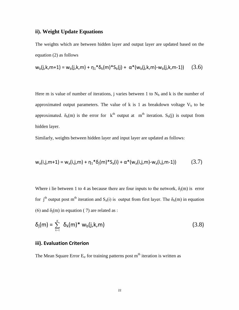
ii). Weight Update Equations

The weights which are between hidden layer and output layer are updated based on the

equation (2) as follows

wb(j,k,m+1) = wb(j,k,m) + η1*δk(m)*Sb(j) + α*(wb(j,k,m)-wb(j,k,m-1)) (3.6)

Here m is value of number of iterations, j varies between 1 to Nh and k is the number of

approximated output parameters. The value of k is 1 as breakdown voltage Vb to be

approximated. δk(m) is the error for kth

output at mth

iteration. Sb(j) is output from

hidden layer.

Similarly, weights between hidden layer and input layer are updated as follows:

wa(i,j,m+1) = wa(i,j,m) + η1*δj(m)*Sa(i) + α*(wa(i,j,m)-wa(i,j,m-1)) (3.7)

Where i lie between 1 to 4 as because there are four inputs to the network, δj(m) is error

for jth

output post mth

iteration and Sa(i) is output from first layer. The δk(m) in equation

(6) and δj(m) in equation ( 7) are related as :

δj(m) =

K

k 1

δk(m)* wb(j,k,m) (3.8)

iii). Evaluation Criterion

The Mean Square Error Etr for training patterns post mth

iteration is written as

23

Etr (m) = (

P

p 1

(Vb1p–Vb2p(m))2)*(1/P) (3.9)

Here, Vb1p is the value determined by the experiment the breakdown voltage used for

purpose of training, Vb2p (m) is the (modeled) value of the breakdown voltage post mth

iteration, P is the value of number of training patterns. The training is halted at the point

when the minimum value of Etr which is taken and this value do not change with the

number of iterations.

iv). Mean Absolute Error

The Mean Absolute Error Ets, is a very good performance measure for determining the

exactness of the ANN System. The Etr determines that how efficiently the network has

adapted to fit to the training data, even if the data is contaminated. On the other front, the

Ets signifies that how efficiently trained network work on a new data set not which

included in the training set.

The Ets for test data expressed in percentage (%) is given by:

Ets = (1/S)* (

S

s 1

|(Vb4s –Vb3s)| / (Vb3s)*100 (3.10)

Here,Vb3s is the experimental value of the breakdown voltage taken for the reason of

testing ,Vb4s is the (modeled value) of the breakdown voltage after testing input data

which is passed in the trained network and S is number of testing patterns.

24

3.2 Back Propagation Algorithm

Backpropagation is a well-known method for teaching artificial neural networks so

as how to do a given task. It was first explained by Arthur E. Bryson and Yu-Chi Ho in

1969, but it was not until 1974, and later, through the work of Paul Werbos, David E.

Rumelhart, Geoffrey E. Hinton and Ronald J. Williams, that it became popular.

It is a method of supervised learning that can be visualized as a generalization of the

delta rule. It demands a teacher that knows, or can find out, the desired output for any

input in training set. It is extremely effective for feedforward networks. The term is an

abbreviation for "backward propagation of errors". Back propagation demands that the

activation function which is used by the artificial neurons has to be differentiable.

For understanding, the back propagation learning algorithm can be divided into two

phases: 1.propagation and 2.weight update.

Phase 1: Propagation

Each propagation module comprises the following steps:

1. Forward propagation of a training data pattern's input through neural network in

order to produce the propagation's output activations.

2. Backward propagation of the propagation's output activations through the neural

network by using training pattern's target to generate the deltas of all output and

hidden neurons.

25

Phase 2: Weight update

For every weight-synapse:

1. The output delta and input activation is to be multiplied to find gradient of the

weight.

2. Bring the weight in the opposite direction of the gradient by subtracting a ratio of

it from the weight.

This ratio has impact on the speed and quality of learning; it is therefore called the

learning rate. The sign of the gradient of a weight signifies that where error is increasing,

because of this the weight has to be updated in the opposite direction.

Perform repetition of the phases 1 and 2 until the performance of the network is

satisfactory.

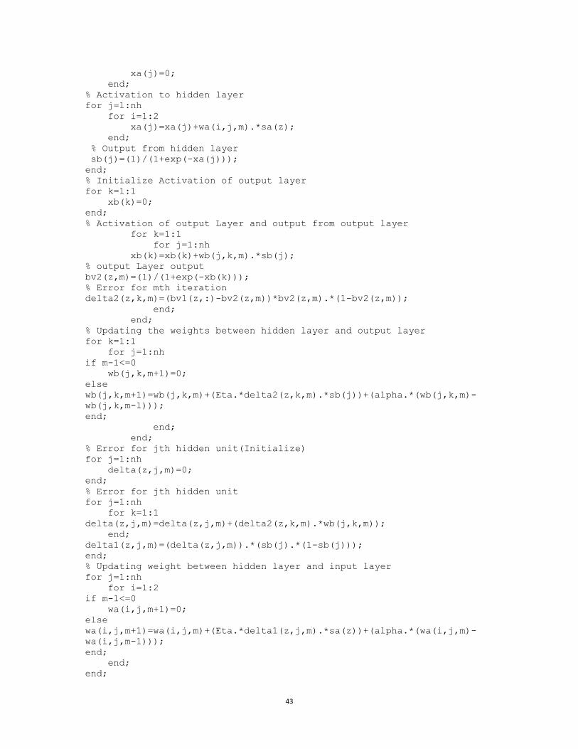
The MATLAB code which is applied to train and test the data sets is given in Appendix I.

The code provided is used for AC conditions by varying the ANN parameters

accordingly and hence the breakdown voltage is found out.

26

CHAPTER 4

MODELING RESULTS

27

Using the MATLAB code and the results for training and testing data sets under both AC

and DC conditions to find out the breakdown voltage of White Minilex paper are

tabulated.

4.1 TABULATION

Table 4.1: Table for training the Neural Network program for AC breakdown voltage for

white Minilex paper.

Sl.

No.

Insulation thickness in

mm

Void Depth in mm

Diameter of void

in mm

Breakdown

voltage in kV

1 0.125 0.125 3 2.3

2 0.125 0.125 4 2.2

3 0.125 0.125 5 2.3

4 0.18 0.125 1.5 2.2

5 0.18 0.125 2 2.2

6 0.18 0.125 4 2.2

7 0.26 0.125 1.5 2.3

8 0.26 0.125 3 2.33

28

Table 4.2: Table for Mean square error by keeping the no. of hidden neurons and

learning rate factor constant and varying the momentum factor (AC)

Sl.no. Nh

(No. of hidden neurons)

α

(Momentum

factor)

Eta

(Learning rate

factor)

MSE

(Mean Square

error)

1. 3 0.4 0.4 1.31523 x 10-4

2. 3 0.5 0.4 9.37144 x 10-5

3. 3 0.6 0.4 5.58897 x 10-5

4. 3 0.65 0.4 3.79286 x 10-5

5. 3 0.7 0.4 2.22842 x 10-5

Table 4.3: Table for Mean square error (Under AC) by keeping the momentum factor

and learning rate factor constant and varying the no. of hidden neurons

Sl.no. Nh

(No. of hidden neurons)

α

(Momentum

factor)

Eta

(Learning rate

factor)

MSE

(Mean Square

error)

1. 4 0.7 0.4 1.25634 x 10-5

2. 5 0.7 0.4 9.25402 x 10-6

3. 6 0.7 0.4 3.66723 x 10-6

29

Table 4.4:Table Mean Square error by keeping the no. of hidden neurons and momentum

factor constant and varying the learning rate factor.

Sl.no. Nh

(No. of hidden neurons)

α

(Momentum

factor)

Eta

(Learning rate

factor)

MSE

(Mean Square

error)

1. 6 0.7 0.5 2.11398 x 10-6

2. 6 0.7 0.6 1.32614 x 10-6

3. 6 0.7 0.65 1.07543 x 10-6

4. 6 0.7 0.7 8.35634 x 10-7

30

Table 4.5: Table to test the Neural Network program for AC breakdown voltage for white

Minilex paper based on the data from tables 2, 3 and 4

RESULT :

Mean Absolute Error (MAE) under AC conditions = 1.7872%

Sl.

No.

Insulation

thickness in

mm

Void Thickness

in mm

Diameter of

void in mm

Experimental

Value of

Breakdown

voltage in kV

Modeled

Value of

Breakdown

voltage in kV

1 0.125 0.125 1.5 2.2 2.16732

2 0.125 0.125 2 2.3 2.21321

3 0.18 0.125 3 2.3 2.22114

4 0.18 0.125 5 2.2 2.17389

5 0.26 0.125 2 2.2 2.18065

6 0.26 0.125 4 2.2 2.18068

7 0.26 0.125 5 2.2 2.18069

31

Table 4.6 : Table to train the Neural Network program for DC breakdown voltage for

white Minilex paper.

Sl.no.

Thickness of

the material

(mm)

Void

Depth(mm)

Void Diameter

(mm)

Mean value of

Breakdown

Voltage(Experim

ental) (kV)

1. 0.125 0.025 1.5 23.44

2. 0.125 0.025 2.0 22.88 3. 0.125 0.025 3.0 23.22 4. 0.125 0.025 4.0 24.44 5. 0.125 0.025 5.0 22.55 6. 0.18 0.025 1.5 23.55 7. 0.18 0.025 2.0 23.22 8. 0.18 0.025 3.0 24.44 9. 0.18 0.025 4.0 23.77

10. 0.18 0.025 5.0 22.88 11. 0.26 0.025 1.5 23.33 12. 0.26 0.025 2.0 23.00 13. 0.26 0.025 3.0 24.44 14. 0.26 0.025 4.0 23.77 15. 0.26 0.025 5.0 23.22 16. 0.125 0.125 1.5 24.44 17. 0.125 0.125 2.0 23.55 18. 0.125 0.125 3.0 22.55 19. 0.125 0.125 4.0 23.22 20. 0.125 0.125 5.0 23.77 21. 0.18 0.125 1.5 23.00 22. 0.18 0.125 2.0 24.33 23. 0.18 0.125 3.0 23.77 24. 0.18 0.125 4.0 22.88 25. 0.18 0.125 5.0 24.33 26. 0.26 0.125 1.5 23.22 27. 0.26 0.125 2.0 23.55 28. 0.26 0.125 3.0 23.44 29. 0.26 0.125 4.0 23.77 30. 0.26 0.125 5.0 22.88

32

Table 4.7: Table for Mean square error by keeping the no. of hidden neurons and

learning rate factor constant and varying the momentum factor (DC)

Sl.no

Nh

(No. of hidden

neurons)

α

(Momentum

factor)

Eta

(Learning rate

factor)

MSE

(Mean square

error)

1. 3 0.4 0.4 2.39483 x 10-4

2. 3 0.5 0.4 1.68282 x 10-4

3. 3 0.6 0.4 9.84504 x 10-5

4. 3 0.65 0.4 6.63633 x 10-5

5 3 0.7 0.4 3.88024 x 10-5

33

Table 4.8: Table for Mean square error (DC) by keeping the momentum factor and

learning rate factor constant and varying the no. of hidden neurons

Sl.no.

Nh

(No. of hidden

neurons)

α

(Momentum

factor)

Eta

(Learning rate

factor)

MSE

(Mean square

error)

1. 4 0.7 0.4 2.02994 x 10-5

2. 5 0.7 0.4 1.44832 x 10-5

3. 6 0.7 0.4 4.96045 x 10-6

34

Table 4.9: Table for Mean Square error by keeping the no. of hidden neurons and

momentum factor constant and varying the learning rate factor.

Sl.no

Nh

(No. of hidden

neurons)

α

(Momentum factor

Eta

(Learning rate

factor)

MSE

(Mean square

error)

1. 6 0.7 0.5 2.68643 x 10-6

2. 6 0.7 0.6 1.58624 x 10-6

3. 6 0.7 0.65 1.24985 x 10-6

4. 6 0.7 0.7 9.98243 x 10-7

35

Table 4.10: Table to test the Neural Network program for AC breakdown voltage for

white Minilex paper based on the data from tables 7, 8 and 9

Sl.no.

Thickness of the

material (mm)

Void Depth

(mm)

Void

Diameter

(mm)

Mean value of

Breakdown Voltage

(Experimental) (kV)

Mean value of

Breakdown

voltage

(Modeled) (kV)

1. 0.125 0.125 1.5 24.44 23.5178

2. 0.125 0.125 2.0 23.55 23.1272

3. 0.125 0.125 3.0 22.55 22.4530

4. 0.125 0.125 4.0 23.22 22.9343

5. 0.125 0.125 5.0 23.77 23.2404

6. 0.18 0.125 1.5 23.00 22.8459

7. 0.18 0.125 2.0 24.33 23.5629

8. 0.18 0.125 3.0 23.77 23.3188

9. 0.18 0.125 4.0 22.88 22.7567

10. 0.18 0.125 5.0 24.33 23.5629

11. 0.26 0.125 1.5 23.22 23.0662

12. 0.26 0.125 2.0 23.55 23.2788

13. 0.26 0.125 3.0 23.44 23.1196

14. 0.26 0.125 4.0 23.77 23.4011

15. 0.26 0.125 5.0 22.88 22.8098

RESULT :

Mean Absolute Error (MAE) under DC conditions = 3.587 %

36

4.2: PLOTTING

Fig 4.1: Variation between the no. of iterations and the mean square error for AC

37

Fig 4.2: Variation between the no. of iterations and the root mean square error for AC

38

Fig 4.3: Variation between the no. of iterations and the mean square error for DC

39

Fig 4.4: Variation between the no. of iterations and the root mean square error for DC

40

CONCLUSION

In this work we have used one of the most sophisticated soft-computing techniques that is

Artificial Neural Networks method. Under both AC and DC conditions the breakdown

voltage of a typical White Minilex paper is predicted using MATLAB 7.1. The values of

mean square error and the mean absolute error show the effectiveness of Multilayer

Feedforward Neural Network in predicting the breakdown voltage.

o The mean square error under AC and DC conditions is in the range of 10^

(-7).

o The Mean absolute error under AC conditions was found out to be

1.7872%.

o The Mean absolute error under DC conditions was found out to be

3.587%.

41

REFERENCES

1. Meek J.M. and Craggs J.D., Electrical Breakdown of Gases. Chichester: John

Wiley & Sons, 1978.

2. Freeman J.A., Skapura D.M., Neural Networks Algorithms, Applications and

Programming Techniques. California: Addison Wesley Publishing Company.

3. Hassoun M.H., Artificial Neural Network. Massachusetts: The MIT Press, 1995

4. Haykin S., Kalman Filtering and Neural Network. California: John Wiley & Sons,

2001.

5. Mohanty S.,Ghosh S. Artificial neural networks modeling of breakdown voltage

of solid Insulating materials in the presence of void, Solid Dielectrics, ICSD '07.

IEEE International Conference, (2007):pp. 94-97.

6. Padhy A., Modeling of Breakdown Voltage of White Minilex Paper in the

presence of voids under AC and DC conditions using Neural Network,

http://ethesis.nitrkl.ac.in/2186/.

7. http://www.codeproject.com/Articles/16419/AI-Neural-Network-for- beginners-

Part-1-of-3.

8. http://en.wikipedia.org/wiki/Feedforward_neural_network .

9. http://en.wikipedia.org/wiki/File:Ann_dependency_graph.png

10. http://article.sapub.org/10.5923.j.ajsp.20110101.01.html

42

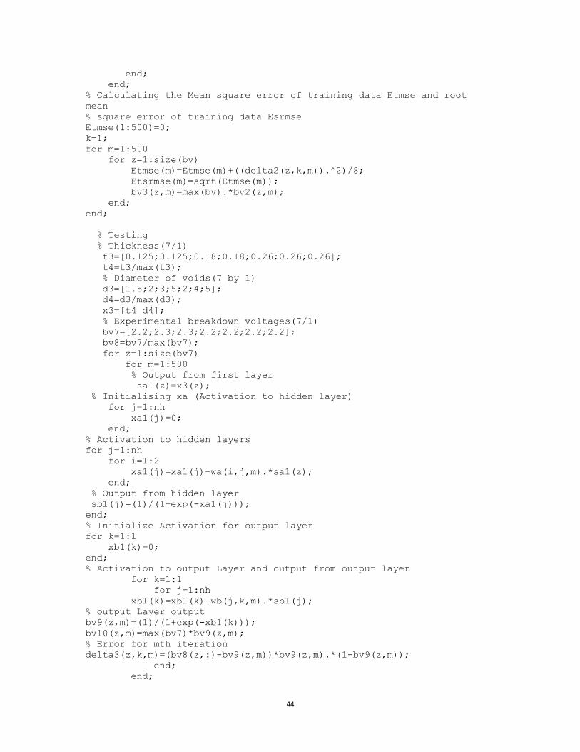
APPENDIX

MATLAB code for modeling of breakdown voltage of White Minilex Paper under

DC and AC conditions.

Clear all;

% ERROR FROM OUTPUT LAYER FEEDBACK TO THE HIDDEN LAYER

% To model the breakdown voltage of White Minilex under AC and DC

conditions as a function of void

% diameter d(mm) & insulation thickness t(mm)

% Backpropagation Algorithm used for modeling

% t1 is void thickness = 0.125mm

% Input Training Patterns 8(8 by 2) (insulation thickness & void

% diameter)

t= [0.125;0.125;0.125;0.18;0.18;0.18;0.26;0.26];

% values of t for training data of DC only

t1=t/max (t);

d=[3;4;5;1.5;2;4;1.5;3];

d1=d/max(d);

x=[t1 d1];

% Output Training Data 8(8 by 1)(Breakdown Voltage Experimental)

bv=[2.3;2.2;2.3;2.2;2.2;2.2;2.3;2.3];

bv1=bv/max(bv);

% initialize Learning Rate Parameter

Eta=0.99;

% initialize Momentum Factor

alpha=0.85;

% initialize hidden neuron numbers

nh=3;

% code for training the neural network & designing it by minimizing the

% error of the training data & also testing the network

% Initialize the weights between input layer & hidden layer, hidden

layer &

% output layer

a1=-1;

b1=1;

rand('state',0);

for k=1:1

for j= 1:nh

for i=1:2

wa(i,j,1)=a1 + (b1-a1).*rand(1,1);

wb(j,k,1)=a1 + (b1-a1).*rand(1,1);

end;

end;

end;

for z=1:size(bv)

for m=1:500

% Output from first layer

sa(z)=x(z);

% Initialize xa (Activation to hidden layer)

for j=1:nh

43

xa(j)=0;

end;

% Activation to hidden layer

for j=1:nh

for i=1:2

xa(j)=xa(j)+wa(i,j,m).*sa(z);

end;

% Output from hidden layer

sb(j)=(1)/(1+exp(-xa(j)));

end;

% Initialize Activation of output layer

for k=1:1

xb(k)=0;

end;

% Activation of output Layer and output from output layer

for k=1:1

for j=1:nh

xb(k)=xb(k)+wb(j,k,m).*sb(j);

% output Layer output

bv2(z,m)=(1)/(1+exp(-xb(k)));

% Error for mth iteration

delta2(z,k,m)=(bv1(z,:)-bv2(z,m))*bv2(z,m).*(1-bv2(z,m));

end;

end;

% Updating the weights between hidden layer and output layer

for k=1:1

for j=1:nh

if m-1<=0

wb(j,k,m+1)=0;

else

wb(j,k,m+1)=wb(j,k,m)+(Eta.*delta2(z,k,m).*sb(j))+(alpha.*(wb(j,k,m)-

wb(j,k,m-1)));

end;

end;

end;

% Error for jth hidden unit(Initialize)

for j=1:nh

delta(z,j,m)=0;

end;

% Error for jth hidden unit

for j=1:nh

for k=1:1

delta(z,j,m)=delta(z,j,m)+(delta2(z,k,m).*wb(j,k,m));

end;

delta1(z,j,m)=(delta(z,j,m)).*(sb(j).*(1-sb(j)));

end;

% Updating weight between hidden layer and input layer

for j=1:nh

for i=1:2

if m-1<=0

wa(i,j,m+1)=0;

else

wa(i,j,m+1)=wa(i,j,m)+(Eta.*delta1(z,j,m).*sa(z))+(alpha.*(wa(i,j,m)-

wa(i,j,m-1)));

end;

end;

end;

44

end;

end;

% Calculating the Mean square error of training data Etmse and root

mean

% square error of training data Esrmse

Etmse(1:500)=0;

k=1;

for m=1:500

for z=1:size(bv)

Etmse(m)=Etmse(m)+((delta2(z,k,m)).^2)/8;

Etsrmse(m)=sqrt(Etmse(m));

bv3(z,m)=max(bv).*bv2(z,m);

end;

end;

% Testing

% Thickness(7/1)

t3=[0.125;0.125;0.18;0.18;0.26;0.26;0.26];

t4=t3/max(t3);

% Diameter of voids(7 by 1)

d3=[1.5;2;3;5;2;4;5];

d4=d3/max(d3);

x3=[t4 d4];

% Experimental breakdown voltages(7/1)

bv7=[2.2;2.3;2.3;2.2;2.2;2.2;2.2];

bv8=bv7/max(bv7);

for z=1:size(bv7)

for m=1:500

% Output from first layer

sa1(z)=x3(z);

% Initialising xa (Activation to hidden layer)

for j=1:nh

xa1(j)=0;

end;

% Activation to hidden layers

for j=1:nh

for i=1:2

xa1(j)=xa1(j)+wa(i,j,m).*sa1(z);

end;

% Output from hidden layer

sb1(j)=(1)/(1+exp(-xa1(j)));

end;

% Initialize Activation for output layer

for k=1:1

xb1(k)=0;

end;

% Activation to output Layer and output from output layer

for k=1:1

for j=1:nh

xb1(k)=xb1(k)+wb(j,k,m).*sb1(j);

% output Layer output

bv9(z,m)=(1)/(1+exp(-xb1(k)));

bv10(z,m)=max(bv7)*bv9(z,m);

% Error for mth iteration

delta3(z,k,m)=(bv8(z,:)-bv9(z,m))*bv9(z,m).*(1-bv9(z,m));

end;

end;

45

% Updating weights between hidden layer and output layer

for k=1:1

for j=1:nh

if m-1<=0

wb(j,k,m+1)=0;

else

wb(j,k,m+1)=wb(j,k,m)+(Eta.*delta3(z,k,m).*sb1(j))+(alpha.*(wb(j,k,m)-

wb(j,k,m-1)));

end;

end;

end;

% Error for jth hidden unit(Initialize)

for j=1:nh

delta4(z,j,m)=0;

end;

% Error for jth hidden unit

for j=1:nh

for k=1:1

delta4(z,j,m)=delta4(z,j,m)+(delta3(z,k,m).*wb(j,k,m));

end;

delta5(z,j,m)=(delta4(z,j,m)).*(sb1(j).*(1-sb1(j)));

end;

% Updating weight between hidden layer and input layer

for j=1:nh

for i=1:2

if m-1<=0

wa(i,j,m+1)=0;

else

wa(i,j,m+1)=wa(i,j,m)+(Eta.*delta5(z,j,m).*sa1(z))+(alpha.*(wa(i,j,m)-

wa(i,j,m-1)));

end;

end;

end;

end;

end;

% Calculating the MAE of test data

MAE=0;

for z=1:size(bv7)

e2(z)=bv7(z)-bv10(z,500);

MAE=MAE +((100/7)*abs(e2(z)/bv7(z)));

end;