Ann. Rev. Plant Physiol. 1976. 27:407-34

MODELING OF

PLANT GROWTH

Ralph O. Erickson 1 Department of Biology, University of Pennsylvania, Philadelphia, Pennsylvania 19174

CONTENTS

-:-7616

GROWTH CURVES .......................................................................................................... 409 MEASUREMENT AND ANALYSIS OF PLANT GROWTH .............................................. 411 GROWTH OF THE PLANT AXIS .......................... .......................................................... 417 GROWTH IN TWO DIMENSIONS.................................................................................... 424 DEVELOPMENTAL INDICES .......................................................................................... 428 SUMMARy........................................................................................................................ 432

The notion of modeling in science has many connotations. There are physical models, such as the atomic models of chemistry which consist of wooden or plastic balls proportional in size to atoms, together with connectors to represent chemical bonds, or realistic sculptures representing the overaIl form or the histology of an organ such as a leaf, etc. In enzyme kinetics, reaction diagrams are frequently used, in which symbols for reactants are connected by arrows to indicate theorized reac­tions. Similar diagrams are also used in less weIl understood areas of plant physi­ology such as the photoperiodic induction of flowering. In many cases a model is in the form of a differential equation, or a system of differential equations, or equations which result from the solution of differential equations, in which the variables and parameters are intended to correspond to measurable attributes and relationships in a system which is being investigated. Recently, logical systems have been proposed to model the development of organisms, the L-systems of Linden­mayer (50, 51), which can be studied by the methods which are used in automaton theory, related to computer applications. There are many other sorts of models, that is to say, more or less abstract representations of natural phenomena. This review will deal primarily with morphogenetic aspects of growth, that is, with dimensions and with the ceIlular aspects of form. Much of the mathematics will therefore be related to geometry. I will be concerned mainly with the use of differential equations

IThe author's research which is referred to here has had the support of grants from the National Science Foundation. Discussions with Dr. Wendy Kuhn Silk, and her generous assistance, have played a crucial part in the conception and completion of this review.

Copyright 1976. All rights reserved 407

Ann

u. R

ev. P

lant

. Phy

siol

. 197

6.27

:407

-434

. Dow

nloa

ded

from

arj

ourn

als.

annu

alre

view

s.or

gby

WIB

6151

- D

euts

che

Fors

chun

gsge

mei

nsch

aft o

n 04

/30/

09. F

or p

erso

nal u

se o

nly.

408 ERICKSON

to model plant growth, since the power of differential equations has been abundantly proven in the physical sciences, and the resources of classical mathematics are available for characterizing and solving them. Highly developed computer methods are also available for finding numerical solutions of differential equations, even when they may be mathematically intractable (57).

When devising a scientific model that is to have explanatory power, it is extremely important that the parameters of the model and the relationships which it expresses correspond with the biological system which is being investigated. In discussing models of growth, I will therefore be at pains to point out the correspondence between features of the model and of the growing structure. As a matter of fact, much of the discussion will center around appropriate expressions of growth rates. I will also discuss methods which can be used to study growth empirically and to analyze growth data in such a way as to make the results amenable to theoretical consideration.

I shall first discuss the growth of entire plants, plant organs, or excised portions of plants, making reference to theoretical growth equations which have been proposed for them. Methods of making growth measurements will be considered, and in particular I will discuss methods of analyzing empirical growth data so as to yield efficient and suitable estimates of growth rates and growth parameters.

For more detailed analysis, particularly of morphogenetic processes, it is impor­tant to consider how growth rates may differ from point to point within the growing system, as in a meristem. To have meaning in a differential equation, data must here be obtained with good spatial resolution as well as good resolution in time. The growth rates estimated from such data should be elemental, that is, they should be stated in terms of differentials of length, area, or volume (dx, dA, or d V) as well as the time differential dt. Following mathematical usage, these differentials of the spatial coordinates are referred to as elements of length, area, and volume, and they appear in elemental rates of change of length, area, or volume. It goes without saying that these rates should also be instantaneous.

Analyses of growth in length, as in a root, in the internode cell of Nitella and other examples will be discussed. In the case of Nitel/a, a model for the regulation of the growth rate of the cell, in the form of two differential equations, will be reviewed.

The elemental analysis of growth in two dimensions will be exemplified by a study of the growth of the lamina of a leaf, and a model for growth in surface of an idealized surface of revolution will be discussed.

The elemental analysis of growth in three spatial dimensions presents formidable difficulties which have not been resolved, as does the analysis in even one or two dimensions of a morphologically complex system such as the shoot apex with its leaf primordia. In such cases, a developmental index is useful in referring detailed measurements or analyses, made, for example, on samples of tissue, or histological preparations, to the time axis and hence to allow estimation of growth rates. Illustra­tions of developmental indices are log bud length in flower development of Lilium and the plastochron index for vegetative shoot development.

Much of the content of this essay is also discussed in another article (20).

Ann

u. R

ev. P

lant

. Phy

siol

. 197

6.27

:407

-434

. Dow

nloa

ded

from

arj

ourn

als.

annu

alre

view

s.or

gby

WIB

6151

- D

euts

che

Fors

chun

gsge

mei

nsch

aft o

n 04

/30/

09. F

or p

erso

nal u

se o

nly.

GROWTH CURVES

MODELING OF PLANT GROWTH 409

In a sense, any equation which is purported to correspond to a living phenomenon can be termed a model of the phenomenon. In discussions of plant growth, many gro�th equations have been put forward in which an attempt is made to account for the increase in size (usually height or weight) of a plant or a plant organ on the basis of simple assumptions. Williams (69-71 ) and Leopold & Kriedemann (49) provide references to some of the literature. In the simplest case, the growth rate may merely be assumed constant, dx/dt = a, where x is a measure of the size (e.g. length) of a plant or plant organ. This obviously leads to a straight line, x = Xo + at. The growth in length of a root or a shoot is often found to be approximately linear over a considerable period of time. Examples are the primary root of Zea, which grows in length linearly at nearly 2 mm.hr-I for 3 days or more, and the shoot of the bamboo Dendrocalamus sp., studied by Kraus (48) , which grew linearly at about 0.28 m.day-I for nearly 2 months. (A native assistant climbed the culm daily with a tape, to a height of 14 m).

Another simple example is Blackman's ( 1 0) proposal of the compound interest law of plant growth. If one assumes that the rate of growth in size x is simply proportional to its size, the assumption can be stated as the differential equation dx/dt = r.x, which has as its solution the simple exponential equation x = xoert, Xo being the size at time t = 0, e the base of natural logarithms, and r a constant which I will term the relative growth rate, since it is the rate of growth in size divided by the size (I/x)(dx/dt). A simple test of the applicability of this equation is suggested by writing it in logarithmic form, In x = In Xo + rt, which is the equation of a straight line. Plotting measurements of x vs t on semilogarithmic graph paper will yield an approximate straight line if the equation is applicable, and a straight line can be fitted by the least squares method. It is often found empirically to fit the early phases of growth in weight, dry weight, length, etc of many plants such as seedlings, sporelings, cuttings, etc. In some cases, exponential growth con­tinues for a long period. For example, the flower buds of Lilium longiflorum grow in length exponentially from the time they can first be measured without injury until 3 or 4 days before anthesis, a period of about a month (I5).

It is usualIy found, however, that if the growth of a plant or a plant organ is followed over a long period, it departs from the simple exponential relationship. For instance, in the growth of a herbaceous plant throughout the growing season, or the growth of a leaf from a primordium to maturity, the plot of size (e.g. length or weight) vs time forms a sigmoid curve. Several equations have been proposed to account for such inflected curves. One, which might be termed the autocatalytic equation, follows from the assumption that the rate of growth in size is proportional to the size attained and to the difference between the size attained and some assumed final size, that is, dx/dt = kx(xJ - x). This is analogous to an assumption that the rate of a chemical reaction is proportional to the amount of product and to the amount of substrate remaining, the first proportionality implying autocatalysis. In the chemical case, xJ is the initial amount of substrate, and in the analogy to plant growth, it is the final size. On integration this is x = xJ/{l + Ce-kl). It may

Ann

u. R

ev. P

lant

. Phy

siol

. 197

6.27

:407

-434

. Dow

nloa

ded

from

arj

ourn

als.

annu

alre

view

s.or

gby

WIB

6151

- D

euts

che

Fors

chun

gsge

mei

nsch

aft o

n 04

/30/

09. F

or p

erso

nal u

se o

nly.

41 0 ERICKSON

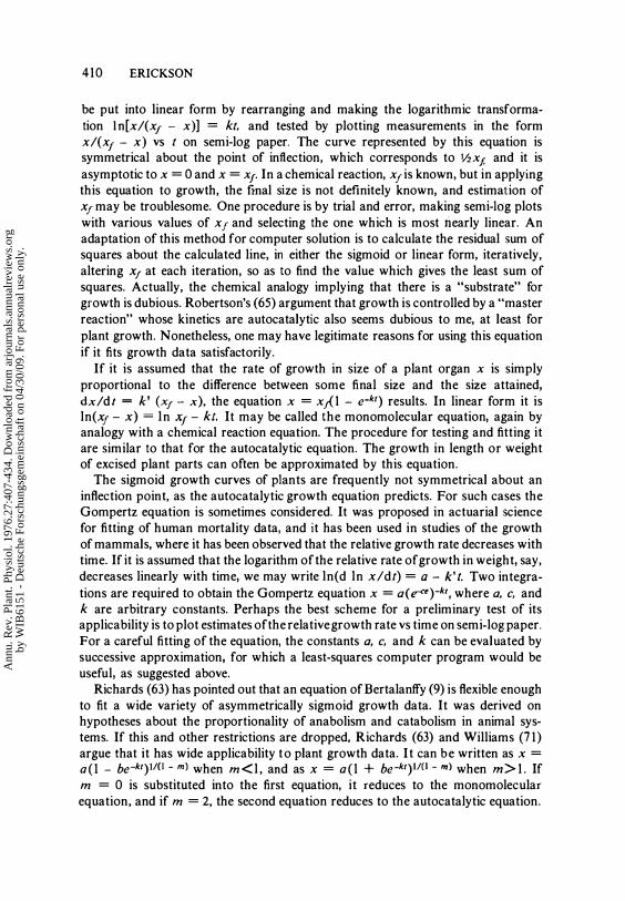
be put into linear form by rearranging and making the logarithmic transforma­tion In[x/(xi - x)] = kt, and tested by plotting measurements in the form x/(xi - x) vs t on semi-log paper. The curve represented by this equation is symmetrical about the point of inflection, which corresponds to lhxj. and it is asymptotic to x = 0 and x = XI' In a chemical reaction, XI is known, but in applying this equation to growth, the fmal size is not definitely known, and estimation of xI may be troublesome. One procedure is by trial and error, making semi-log plots with various values of x I and selecting the one which is most nearly linear. An adaptation of this method for computer solution is to calculate the residual sum of squares about the calculated line, in either the sigmoid or linear form, iteratively, altering XI at each iteration, so as to find the value which gives the least sum of squares. Actually, the chemical analogy implying that there is a "substrate" for growth is dubious. Robertson's (65) argument that growth is controlled by a "master reaction" whose kinetics are autocatalytic also seems dubious to me, at least for plant growth. Nonetheless, one may have legitimate reasons for using this equation if it fits growth data satisfactorily.

If it is assumed that the rate of growth in size of a plant organ X is simply proportional to the difference between some final size and the size attained, dx/d t = k' (XI - x), the equation x = xII - e-kt) results. In linear form it is In(xi - x) = In XI - kt, It may be called the monomolecular equation, again by analogy with a chemical reaction equation. The procedure for testing and fitting it are similar to that for the autocatalytic equation. The growth in length or weight of excised plant parts can often be approximated by this equation.

The sigmoid growth curves of plants are frequently not symmetrical about an inflection point, as the autocatalytic growth equation predicts. For such cases the Gompertz equation is sometimes considered. It was proposed in actuarial science for fitting of human mortality data, and it has been used in studies of the growth of mammals, where it has been observed that the relative growth rate decreases with time. If it is assumed that the logarithm of the relative rate of growth in weight, say, decreases linearly with time, we may write In(d In x/dt) = a - k't. Two integra­tions are required to obtain the Gompertz equation x = a(r<)-kt, where a, c, and k are arbitrary constants. Perhaps the best scheme for a preliminary test of its applicability is to plot estimates of the relative growth rate vs time on semi-log paper. For a careful fitting of the equation, the constants a, c, and k can be evaluated by successive approximation, for which a least-squares computer program would be useful, as suggested above.

Richards (63) has pointed out that an equation of Bertalanffy (9) is flexible enough to fit a wide variety of asymmetrically sigmoid growth data. It was derived on hypotheses about the proportionality of anabolism and catabolism in animal sys­tems. If this and other restrictions are dropped, Richards (63) and Williams (7 1) argue that it has wide applicability to plant growth data. It can be written as x = a ( 1 - be-kt)l/O - m) when m<l , and as x = a ( 1 + be-kt)l/O - m) when m>1 . If m = 0 is substituted into the first equation, it reduces to the monomolecular equation, and if m = 2, the second equation reduces to the autocatalytic equation.

Ann

u. R

ev. P

lant

. Phy

siol

. 197

6.27

:407

-434

. Dow

nloa

ded

from

arj

ourn

als.

annu

alre

view

s.or

gby

WIB

6151

- D

euts

che

Fors

chun

gsge

mei

nsch

aft o

n 04

/30/

09. F

or p

erso

nal u

se o

nly.

MODELING OF PLANT GROWTH 411

If m = I the equations cannot be solved, but Richards (63) shows that as m approaches I from either side, the limiting form of the equation is the Gompertz equation. The flexibility of this function depends on its containing four arbitrary constants, which as above might be evaluated by successive approximation. Wil­liams (71) provides an example of fitting of this function to data on the growth in length of leaves of flax, Linum usitatissimum.

Even though the hypotheses (differential equations) underlying these equations may not be pertinent to the growth of a plant system, and may therefore be of little theoretical value, they may legitimately be used as arbitrary functions to fit data for the purpose of estimation or prediction. If this is one's intent, it might be that other exponential, trigonometric, or hyperbolic functions could be useful. Functions known as rational, and in particular polynomial equations (59), are especially useful as arbitrary functions for these purposes since they can be evaluated by fairly simple numerical procedures, and the statistics of polynomials is well understood.

MEASUREMENT AND ANALYSIS OF PLANT GROWTH

In studying the growth of a plant or some part of the plant, such as the aerial shoot, the root system, a leaf, or an excised part such as a coleoptile segment, the experi­mental procedures are usually quite simple. For linear dimensions all that is usually needed is a rule, tape, or caliper, though for some purposes a more sensitive device may be needed, as in the study by Evans & Ray (26) of rapid responses of Avena coleoptiles to added auxin. Sometimes it .is useful to make photographs and to obtain measurements from them. Linear measurements can usually be made without injury to the plant, and one can make repeated measurements of the same plant or organ. Plotting such measurements vs time yields growth curves which apply to individu­als. Such data have been termed Type A by Kavanagh & Richards (46), and in studies of human growth are curiously known as ".longitudinal."

For measurements such as fresh weight and dry weight, the procedures are also simple. Frequently interest centers on measurements such as the content of the plant or its part, of protein, chlorophyll, etc, for which a chemical analysis is required that may be simple or more complex. Or histological preparations may be made, perhaps for the study of cellular processes. From the present point of view, the essential characteristic of many such measurements is that they are destructive, and a mea­surement of a given plant or part cannot be repeated. In order to obtain a growth curve for such measurements, one must resort to the statistical procedure of sam­pling from a population of similar plants growing under similar conditions, taking precautions to assure that sampling is random. For instance, a randomized block design might be desirable for a growth study. It is interesting to note that the development of classical small sample statistics, largely by Fisher (27), had its impetus from related problems which arise in agricultural crop testing. Where this statistical sampli�g procedure must be used, the data are sometimes called "cross­sectional," and Kavanagh & Richards (46) spoke of them as Class C data. If type A data are to be obtained for a number of similar plants, sampling questions also

Ann

u. R

ev. P

lant

. Phy

siol

. 197

6.27

:407

-434

. Dow

nloa

ded

from

arj

ourn

als.

annu

alre

view

s.or

gby

WIB

6151

- D

euts

che

Fors

chun

gsge

mei

nsch

aft o

n 04

/30/

09. F

or p

erso

nal u

se o

nly.

412 ERICKSON

arise, and Kavanagh & Richards distinguish this situation as Class E. As they observed, the problem of making efficient estimates of growth parameters from Class E data presents some statistical problems which have not been resolved.

However growth data are obtained, it is almost always desirable to analyze them in such a way as to estimate growth rates. These should be interpretable as deriva­tives, as defined in the differential calculus, rather than in any of the less desirable ways which have sometimes been used. The reason for this is that in any attempt at modeling it should be possible to relate the experimental data to the differential equations which represent the process being modeled. If x is a measured attribute of a plant or organ, its growth curve can be viewed as a function of time x =

f(t). Frequently the first derivative, dx/dt, is of interest, and I will refer to it as the absolute growth rate. In some cases, the absolute rate is found to be approxi­mately constant over some period of time, but more often it is found to vary continuously. In either case, it is often instructive to plot out the absolute rate vs time, in addition to plotting the growth curve.

As Briggs, Kidd & West (I I ) proposed, the relative growth rate is frequently a very appropriate way to express plant growth data, for heuristic reasons given below. Considering the measured attribute x to be a function of time x = f(t), the relative or specific growth rate is (I/x)(dx/dt). It can also be expressed as d In x/dt. One reason for the desirability of the relative rate is the same as stated above, that it often appears in useful differential equations. Another follows from the fact that, to an approximation at least, the rate of deposition of dry matter by a growing green plant is proportional to the bulk of its photosynthetic tissue, and this in turn is roughly proportional to its fresh or dry weight. This reasoning led Blackman ( 10) to propose the term "efficiency index" for the relative growth rate, and led to other formulations of growth rates such as the leaf specific rate, in which the absolute rate, dx/dt, usually for increase in dry weight, is divided by the total leaf area of a shoot ( 10, 49, 69). Furthermore, since the dimension of the relative rate is simply time -I, direct comparisons may be made of the relative rates of change of any measured attributes of the growing system.

The estimation of growth rates from experimental data often presents some problems because, while growth is continuous, measurements are for practical reasons made only at intervals, and errors arising from the measurement, from imperfect control of growing conditions, or from the sampling procedure used, are always present. These errors are propagated into the estimated rates. To see this in a simple case, assume that measurements of length Xi have been made at equal intervals of time fl.!, and that rates are estimated as increments of Xi divided by the time increment fl.x/fl.!, or (Xi+1 - X;}/(ti+1 - t;). We make the usual assumption in regression analysis, that t, and hence fl. t, are free of error. If the measurement error of Xi is represented by (T i, then the standard deviation of the increments of Xi is (T"x = «(Ti�1 + (T� - 2p(Ti(Ti+l)'i2, or assuming that errors of successive Xi are un correlated (p = 0), this equation is (T /h = (2(T�r". That is, the standard deviation of increments of Xi is greater than that of Xi. This is in keeping with one's usual experience that plots of fl.x/ tl t vs t are more or less erratic (Figure I C). If

Ann

u. R

ev. P

lant

. Phy

siol

. 197

6.27

:407

-434

. Dow

nloa

ded

from

arj

ourn

als.

annu

alre

view

s.or

gby

WIB

6151

- D

euts

che

Fors

chun

gsge

mei

nsch

aft o

n 04

/30/

09. F

or p

erso

nal u

se o

nly.

MODELING OF PLANT GROWTH 413

the measurements have not been made at equal intervals of time, further problems of estimation arise.

If the estimation of growth rates by calculating increments is not satisfactory, the original data may be smoothed, and rates of change of the smooth curve may be estimated in some way. The smoothing may be done by drawing a curved line through a graph of the data by eye ("eyeballing it"), or a growth function may be fitted to the data by a method suggested above. The function may be quite arbitrary. A third method is to use the numerical smoot�ing and differentiation formulas described below.

If an eye-fitted curve has been drawn, slopes can be estimated by the construction method described in analytical geometry, drawing straight lines tangent to the curve at selected points. Each of these lines can be viewed as the hypotenuse of a right triangle with legs parallel to the axes. If the altitude of the triangle is a and its base b, the slope of the line is a /b. If measurements Xi were plotted vs ti, the absolute rate (dx/d t) i at a point is proportional to the slope, the proportionality depending on the scaling of the x- and t-axes of the graph. The relative rate ( lIx)(dx/dt) can be gotten by dividing each estimate of dx/dl by corresponding x. Alternatively, In Xi can be plotted vs ti' and this same graphical procedure used to estimate the relative rate as d In x/d/. It is usually more convenient to use a protractor, adjusting its base line to be tangent to the curve at selected points, and reading the angle <p which the tangent line makes with the abscissa. The slope is tan <p. Richards & Kavanagh (64) describe a convenient double prism devise, a Tange�tmeter, for this purpose. We have made a protractor which is graduated directly in units of tan <p rather than degrees, which makes it unnecessary to look up or compute tan <p (23). Highly developed data-recording equipment, adapted for computer applications, is also available for measuring angles, and can be had from several manufacturers. For careful work, however, these graphical methods lack objectivity and reproduc­ibility.

If a growth equation is used to smooth data, the equation can be differentiated to give explicit equations for the absolute growth rate dx/dt and the relative growth rate d I n x/dr. These equations, written with the parameters found by fitting the data, can then be solved at selected times. However, my experience has been that there is often some bias in these estimates if the equation has been fitted to data covering an extended period of time. This bias stems from systematic discrepancies between the growth equation and the empirical data.

Smoothing formulas ( 1 , 59) and formulas for the first derivative may be based on the least squares fitting of polynomials to empirical data. For growth data we may consider the polynomial Xi = a+blti+bzr2+b3t3+ . . . , fitted to measurements I I Xi at various ti' and its first derivative (dx/dt)i = bl + 2 bzt; t + 3 b3tZ . . . , and I digress to consider the properties of such polynomials. The symbol Xi represents a calculated or smoothed value, as distinct from a measurement Xi' The degree of the polynomial is arbitrary. Thus, if the first two terms are taken', the function is linear; if the first three terms are used, it is quadratic; and there are polynomials of third degree, fourth degree, etc. Methods for fitting polynomials have been highly sys-

Ann

u. R

ev. P

lant

. Phy

siol

. 197

6.27

:407

-434

. Dow

nloa

ded

from

arj

ourn

als.

annu

alre

view

s.or

gby

WIB

6151

- D

euts

che

Fors

chun

gsge

mei

nsch

aft o

n 04

/30/

09. F

or p

erso

nal u

se o

nly.

414 ERICKSON

tematized, in particular by the use of orthogonal polynomials (47). When values of the independent variable, Ii in our application, are equally spaced, the coefiicients of a polynomial take the particularly simple form of a sum of products of the Xi by tabulated values of orthogonal polynomials, divided by a tabulated divisor (7). Tables of these polynomials are available for fitting polynomials up to the fifth degree, to any number of data points from 3 to 75 (2 8, 66). If one carries out the least squares fitting of a polynomial to a certain number n of equally spaced Ii and corresponding X,> symbolically instead of numerically, and solves for Xi' a series of n smoothing formulas results. These are similar in appearance to orthogonal polynomials, giving a series of multipliers and a divisor, which allow Xi to be calculated readily from given Xi' A number of these formulas are published (1, 59) and some are listed in abbreviated form in Table 1. As an example, the quadratic smoothing formula for the third of five points is Xi = (-3X i_2 + 1 2X i_l + 1 7 Xi + 1 2x i+I-3x i+2)/35 . Applying linear formulas of this sort is equivalent to the familiar process of calculating running averages, but the linear formulas have the drawback that they do not accommodate as well to curvature as do the quadratic and higher degree formulas. In practice, a formula is applied to a limited odd number of points, e.g. 3, 5, or 7. A "centered" formula should be used for all the Xi in a column except for the first and last (n-I)/2 points. For example, if the formula quoted above is applied to the 5 points centered on (ti' Xi), Xi is calculated.

Then advance one space and apply the formula again. For the beginning and end points the noncentered formulas are used, but they sometimes give erratic results. If one is working with an ordinary desk calculator, it is helpful to write the coeffi­cients of a formula in a column at the edge of a card with the same spacing as the column of Xi on one's data sheet, and to move the card down one step for each Xi' This process is tedious since it requires entering each Xi value repeatedly. Programming it for a computer is a very simple matter, and it can also be ,;arried out efficiently with a programmable desk or hand-held calculator with several storage registers. Some judgment is required in the use of these formulas, perhaps choosing those formulas which give the least amount of smoothing that will serve one's purpose.

Smoothing by this procedure is illustrated in Figure I , using data of Williams (70) on increase of dry weight of field-grown wheat, Class C data. In Figure IA is shown the smoothed curve calculated with the 5-point quadratic smoothing formula of Table 1 . In Figure I B, logarithms of tIle dry weights have been fitted with the same 5-point smoothing formulas. In both Figure IA and B, the curves follow the points more closely than do the autocatalytic and polynomial equations which Williams (70) fitted. The effect has been merely to remove some of the variability from the data. If one desired, one could calculate the standard error of estimate for each Xi' using a standard formula from regression analysis, but this scarcely seems worth while in many applications.

Numerical differentiation formulas are found in the same way as the smoothing formulas, solving for (dxldt)j instead of Xj. Since dxldt has the dimension of time-1 as well as the dimension of x, the spacing along the time axis tlt must be considered. This appears in the denominators of the formulas as h. The published

Ann

u. R

ev. P

lant

. Phy

siol

. 197

6.27

:407

-434

. Dow

nloa

ded

from

arj

ourn

als.

annu

alre

view

s.or

gby

WIB

6151

- D

euts

che

Fors

chun

gsge

mei

nsch

aft o

n 04

/30/

09. F

or p

erso

nal u

se o

nly.

Table I Smoothing and numerical differentiation formulas based on least squares fitting of polynomials to 3,5, or 7 points (xi' Yi)' where xi are equally spaced with interval h a

Smoothing formulas Linear, 3 points: Yi-I = ( 5 +2 -1)/6 2nd degree, 3 points: Yi-I =( 4-1+1)/3 Linear, 5 points:

Yi-2 = ( +2 +1 -1)/5

Yi-l = ( 4 +3 +2 +1 )/10

Yi = ( +1 +1 +1 +1)/5

Yi+l = ( +2 +3 +4)/10

Yi+2 = ( -1 +1 +2 +3)/5

Numerical differentiation formulas Linear, 3 points: y' = (-1 +0 +1)/2h 2nd degree, 3 points: Yl-l = (-3 +4 -1)/2h 2nd degree, 5 points: Yl-2 = (-54 + 13 +40 +27 -26)/70h

y'i-l =(-34 +3+20+17 -6)/7011

Yf = ( -2 -1 +1 +2)/1011

Yl+l = ( 6 -17 -20 -3 +34)/7011

Yf+2 = ( 26 -27 -40 -13 +54)/70h

Yi = ( 1 + 1 + 1)/3

Yi=( 1+1+1)/3 2nd degree, 5 points:

Yi-2 = ( 31 +9 -3

Yi-I=( 9 +13+12 Yi =( -3 +12+17

Yi+I=( -5 +6+12

Yi+2 = ( 3 -5 -3

-5 +6

+12 +13

Yi+ I = (-I +2 +5)/6

Yi+1 =( 1-1+4)/3

+3)/35 -5)/35 -3)/35 +9)/35

+9 +31)/35

2nd degree, 7 points:

Yi-3 = ( 32 +15 +3 -4 -6 -3 +5 )/42

Yi-2 = ( 5 +4+3 +2 +1 -I )/14

Yi-l = ( 1 +3+4 +4 +3+1 -2)/14

Yi = ( -2 +3 +6 +7 +6 +3 -2)/21

Yi+I' Yi+2' Yi+3' by symmetry

Linear,S points: y' = (-2 -1 +0 +1 +2)/10h

Yl= (-1 +0 +1)/2h Yl+1 = ( 1 -4 +3)/2h 3rd degree, 5 points: Yl-2 = (-125 +136+48 -88 +29)/84h

y'i-I = ( -19 -1 +12 +13 -5)/42h y'; = ( 1 -8 +8 -1)/121z

y'i+l = ( 5 -13 -12 +1 +19)/42h y'i+2 = ( -29 +88 -48 -136 +125)/84h

2nd degree, 7 points:

Yt-3 = (-13 -2 +5 +8 +7 +2 -7)/28h

yt-2 = (-29 -6 +9 +16 +15 +6 -11)/84h

y'i-l = (-19 -6 +3 +8 +9 +6 -1)/841z

Y'i = ( -3 -2 -1 +1 +2 +3)/28h Y';+l' Yl+2' Yf+3' by symmetry

aOnly the coefficients of Y; are given. Smoothed values are Y;;Yl is dY;/dx.

s:: o t) trl t""' Z o o 'T1 '" t""' ;I> Z ...., o � :E ...., ::r:

.j::>. -VI

Ann

u. R

ev. P

lant

. Phy

siol

. 197

6.27

:407

-434

. Dow

nloa

ded

from

arj

ourn

als.

annu

alre

view

s.or

gby

WIB

6151

- D

euts

che

Fors

chun

gsge

mei

nsch

aft o

n 04

/30/

09. F

or p

erso

nal u

se o

nly.

416 ERICKSON

E ",6

"7.., III .. �

10

E 5 '"

o

A

c

t - Time in weeks 25

_1 8 E 2! � 1 .;;; � �.1

C

.01

D 4

-" .. ., �

�I- 2

:;;-0

0

0 10 15 20 25

Figure 1 Dry weights of field-grown wheat (70). A. Curve fitted to points with 5-point quadratic smoothing formulas (Table 1). B. Curve fitted to log dry weight with the same 5-point smoothing formulas. C. Bar diagram (�x/�t) and absolute rate of increase in dry weight (dx/dt) estimated with 5-point quadratic formulas for the first derivative (Table 1). D. Relative rate of increase in dry weight (d In x/dt) estimated with the same 5-point formulas (or numerical differentiation.

differentiation formulas ( 1 , 59) are derived from polynomials which pass precisely through the points to which they are fitted, leaving no degrees of freedom for error estimates, and hence having no smoothing effect. They could be applied to previ­ously smoothed data, but it seems more efficient in dealing with empirical data to use formulas for estimating the derivative which also provide some smoothing. Some such formulas are given in Table 1, and I can provide others. They are used in the same way as the smoothing formulas, except that h must be specified. Their applica­tion to the data on wheat plants is illustrated in Figure 1 C, where estimates of the absolute rate dx/dt are plotted vs t as a smooth curve, and in Figure 10, showing estimates of the relative rate of increase in dry weight, din x/d/. Both curves were obtained with the 5-point quadratic differentiation formulas given in Table 1, ap­plied in the first case to the original values of dry weight Xi' and for the second curve to the natural logarithms In Xi. Alternatively, the relative rate might have been calculated by dividing each estimate, dx,Jdt, by Xi or Xi. The results would differ slightly from those plotted.

Ann

u. R

ev. P

lant

. Phy

siol

. 197

6.27

:407

-434

. Dow

nloa

ded

from

arj

ourn

als.

annu

alre

view

s.or

gby

WIB

6151

- D

euts

che

Fors

chun

gsge

mei

nsch

aft o

n 04

/30/

09. F

or p

erso

nal u

se o

nly.

MODELING OF PLANT GROWTH 417

GROWTH OF THE PLANT AXIS In the preceding section methods were suggested for the accurate estimation of growth rates of entire plants and plant organs from measurements of various kinds. Now I will describe a more detailed analysis in which both the spatial and temporal components of growth rate are analyzed, growth along a plant axis, which is essentially one-dimensional growth. It will be seen that, while more elaborate meth­ods of measurement may be required, the methods of estimation of rates described above are directly applicable. A good example is growth of a root (21, 29, 30, 39). In our experiments (23), roots of Zea mays seedlings were marked with particles of carbon (lamp black) and photographed through a slit onto a moving strip of film to produce streak photographs such as Figure 2. Hejnowicz & Erickson (40) used fluorescent particles, and List (52) utilized reflections of light from epidermal cells of the root to produce similar streak photographs. Goodwin & Stepka (30) and Goodwin & Avers (29) measured positions of cross walls of epidermal cells micro­scopically to obtain similar records. If one takes the distance of a point on the root from the tip of the meristem (or the root cap) as x, streak photographs such as Figure 2 constitute automatic plots of distance x vs time t. Slopes of the streaks can be measured, using the tangent protractor, for example, and these slopes are propor­tional to rates of displacement of points from the tip dx/dt = x' . If these are plotted vs x (Figure 3), they can be interpreted as growth rates of apical segments of the root of length x. The velocity dx/dt can also be taken as proportional to an element of length of the root dx, so that if dx/dt were plotted vs t, the resulting graph could be interpreted as a growth curve of a length element dx. This curve has a markedly asymmetrical sigmoid shape with a prolonged period of slow in­crease, then a sharp acceleration, and a sudden cessation of growth (23).

It is more instructive to estimate the rate of growth of a length element dx. The appropriate expression is dx'/dx, and I have termed it the relative elemental rate of elongation. It can also be interpreted as the one-dimensional case of the diver­gence of the velocity vector div v of vector analysis. It can be estimated from the data of Figure 3, where x' is represented as a function of x, by means of numerical differentiation formulas (Table 1) , taking x as the independent and x' as the depen­dent variable. Relative elemental rates of elongation, dx'/dx, estimated from a number of streak photographs like Figure 2, are plotted as a solid line in Figure 4. Under our experimental conditions, the divergence rises from 0 at the tip of the root, to a maximum of about 0.4 hr-1, 4 mm from the tip, and declines to 0 at about 8 mm. This contrasts greatly with the conclusion drawn from marking experiments by Julius Sachs and many later authors that the maximum rate of elongation is much nearer to the tip. The flaw in these experiments is that the rates estimated are neither elemental nor instantaneous. The single curve (solid line) of Figure 4 suffices to describe the pattern of elongation of an element of the root, if one assumes that the growth pattern is time invariant. In general, we would assume that the velocity of displacement of a point is a function of both time and position, x' = fix, t). Then dx' = (ax'/ax)dx + (ax'/at)dt. If we assume time in variance, then ax'/at = 0,

Ann

u. R

ev. P

lant

. Phy

siol

. 197

6.27

:407

-434

. Dow

nloa

ded

from

arj

ourn

als.

annu

alre

view

s.or

gby

WIB

6151

- D

euts

che

Fors

chun

gsge

mei

nsch

aft o

n 04

/30/

09. F

or p

erso

nal u

se o

nly.

41 8 ERICKSON

2

hrs ---+­I 2 4

Figure 2 Root growth. Streak photograph recording the displacement of marks placed on a growing root of Zea mays (23).

and dx'/dx = ax'/ax, so that one curve suffices. This is approximately true for a considerable period of root growth. but is not so for the initial stages. for very long roots which are approaching the end of their period of growth, nor for some experimentally treated roots. List (52) has described an oscillatory aspect of root growth which also requires a modification of this assumption of time invari­ance.

Although this analysis is one-dimensional. the growth data from the streak photo'­graphs can be used indirectly to estimate the rates at which other processes are

Ann

u. R

ev. P

lant

. Phy

siol

. 197

6.27

:407

-434

. Dow

nloa

ded

from

arj

ourn

als.

annu

alre

view

s.or

gby

WIB

6151

- D

euts

che

Fors

chun

gsge

mei

nsch

aft o

n 04

/30/

09. F

or p

erso

nal u

se o

nly.

� 2.0 L: " E .5 -c: Q) E Q) u o

1.5

� 1.0 "'0 "t­o Q) -o 0:: 1

�I�

0.5

MODELING OF PLANT GROWTH 419

I ] " " ,---------

------------

-

- --- 1

:'/ �

,// 1

5 '0 15

x- Distance from tip (mm)

Figure 3 Root growth. Rates of displacement of points from the tip (dx/dt) estimated from streak photographs.

occurring. For instance, we have estimated the rate of increase in cell number from cell counts of macerated segments of roots (24). If e is the total number of cells in an apical portion of the root of length x. then the number of cells in a segment of length !lx is !le and the data can be plotted as !lel!lx (Figure 5). A smooth curve fitted to this bar diagram such that the area under each segment of the curve equals the area of the corresponding bar can be construed as a graph of deldx vs x. This procedure is justified on the assumption that e and x can be taken as parametric functions of t. and therefore that e is' a function of x alone, e = j(x), just as x' was taken as a function of x alone. Multiplying these estimates of dcldx by corresponding estimates of dxldt gives deldt (= e'), the absolute rate at which cell number of an apical segment is increasing. For the entire meristem which consists of over 250,000 celIs in a Zea root, new celIs are being formed at the rate of about 18,000 celIs-hrl. The relative elemental rate of celI formation de'/de can also be evaluated. If deldt is taken as a function of x. numerical differentiation will give values of de'/dx. and these may be divided by de/dx to yield estimates of de'/de. This rate peaks at about 0. 1 6 hr-I, 1 .25 mm from the tip of the root, as shown by the dotted lines in Figure 4.

We have also made measurements of cell length of randomly chosen cells in longitudinal sections of root segments, and calculated the mean cell length Lc at various distances from the tip. Numerical differentiation gives dLJdx. and again

Ann

u. R

ev. P

lant

. Phy

siol

. 197

6.27

:407

-434

. Dow

nloa

ded

from

arj

ourn

als.

annu

alre

view

s.or

gby

WIB

6151

- D

euts

che

Fors

chun

gsge

mei

nsch

aft o

n 04

/30/

09. F

or p

erso

nal u

se o

nly.

420 ERICKSON

V> Q) a �

CJ U 0 -- c C Q) .... E CJ Q)

.!:l Q) E ::l c: Q)

> -0

§ � 0::

:f:

0.3

I I 0.2 :,

o.lf[ /!{ : I, '. : I I ., • I .

t I I f

I

: I / �.

o . '0; v .) .... t.. ..... . , . . . .. ' .. .. .I . .... ' .... J ••• � ...... >i�.,' 5 10

X - Distance from tip (mm)

-.SlL. dx L�

� dc'

de-F' � Fe

15

Figure 4 Root growth. Relative elemental rates of elongation (dx'/dx) and of cell formation (dc'/de) and relative rates of change in average eell length (II Lc) (dLJdt) and number of files of cells (II FJ (dFcldt).

multiplying these estimates by corresponding dxldt and dividing by Lc yields values of the relative rate of cell elongation (1/ Lc)(dLJdt) (Figure 4, longer dashes). Note that this is not an elemental rate since it pertains to cells, the biological units of plant structure. Cells are microscopic, to be sure, but they are not infinitesi­mal. For the most part the cells are arranged in longitudinal files, cell divisions being predominantly at right angles to the root axis. The files, however, merge and converge on the initial region of the apical meristem of the root, since this is where all the cells of the root originate. The number of files of cells Fe is therefore a function of distance from the tip, and this was estimated by counting the numbers of cells which can be seen in transverse sections of roots. The relative rate of change in number of files, estimated as already described, is plotted as a fine dotted line below the abscissa in Figure 4.

The rates described above can be related to each other by considering a formula which has sometimes been used to estimate cell number in samples of plant tissue (6) in which cells are arranged in longitudinal files. If !:i.x is the length of a segment of tissue (root, internode, coleoptile, etc) being sampled, Lc is the mean cell length, and Fe is the number of files of cells in the segment, then the number of cells

Ann

u. R

ev. P

lant

. Phy

siol

. 197

6.27

:407

-434

. Dow

nloa

ded

from

arj

ourn

als.

annu

alre

view

s.or

gby

WIB

6151

- D

euts

che

Fors

chun

gsge

mei

nsch

aft o

n 04

/30/

09. F

or p

erso

nal u

se o

nly.

E E

�.IOO,OOO

.... o

... (I)

.0 5 r: 0,000 :J

Z I

�I� ��

.

�I� ��

x- Distance 5

MODELING OF PLANT GROWTH 421

100,000

10 15 from tip (mm)

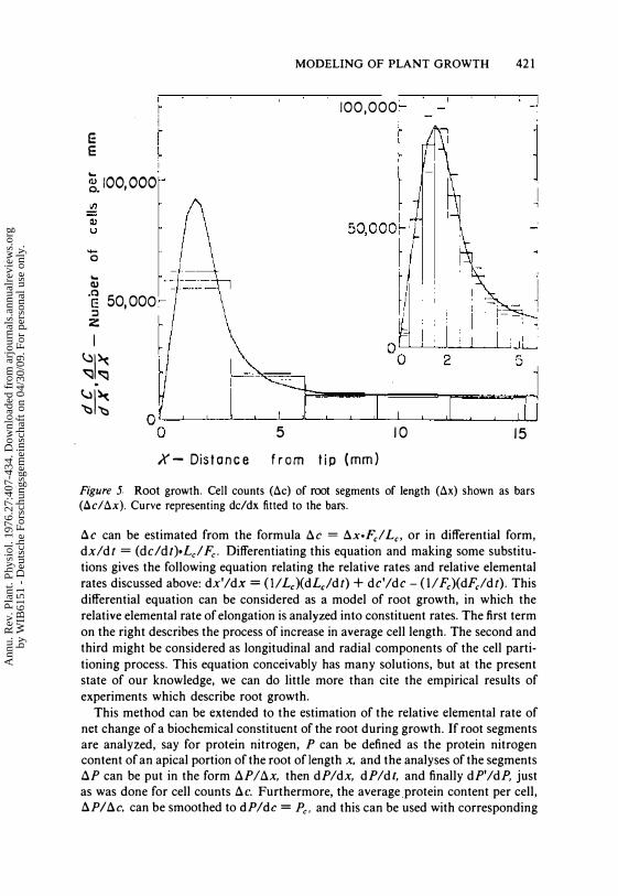
Figure J Root growth. Cell counts (toc) of root segments of length (tox) shown as bars (tocltox). Curve representing dc/dx fitted to the bars.

!::.C can be estimated from the formula !::.e = !::.xoFel Le, or in differential form, dxldt = (deldt)oLcl Fc- Differentiating this equation and making some substitu­tions gives the following equation relating the relative rates and relative elemental rates discussed above: dx'/dx = (1/ LJ(dLJdt) + de'/de - (II Fe)(dFeldt). This differential equation can be considered as a model of root growth, in which the relative elemental rate of elongation is analyzed into constituent rates. The first term on the right describes the process of increase in average cell length. The second and third might be considered as longitudinal and radial components of the cell parti­tioning process. This equation conceivably has many solutions, but at the present state of our knowledge, we can do little more than cite the empirical results of experiments which describe root growth.

This method can be extended to the estimation of the relative elemental rate of net change of a biochemical constituent of the root during growth. If root segments are analyzed, say for protein nitrogen, P can be defined as the protein nitrogen content of an apical portion of the root of length x, and the analyses of the segments !::.P can be put in the form f:..PI!::.x, then dPldx, dPldt, and finally dP'/dP, just as was done for cell counts !::.c. Furthermore, the average .protein content per cell, f:..PI!::.e. can be smoothed to dPlde = Pc, and this can be used with corresponding

Ann

u. R

ev. P

lant

. Phy

siol

. 197

6.27

:407

-434

. Dow

nloa

ded

from

arj

ourn

als.

annu

alre

view

s.or

gby

WIB

6151

- D

euts

che

Fors

chun

gsge

mei

nsch

aft o

n 04

/30/

09. F

or p

erso

nal u

se o

nly.

422 ERICKSON

values of dxldt from the streak photograph analysis to estimate (1/ Pc)(dPcldt), as was done for Le, the average cell lengths. Erickson & Goddard (21) presented such rate estimates for fresh weight, dry weight, total nitrogen, protein nitrog�:n, cell wall constituents, and for crude analyses of the nucleic acids, with highly suggestive results. Unfortunately, this work has not been verified nor extended .

A more direct view of the role of cell divisions at the root meristem is given by Goodwin & Avers' (29) study of Phleum pratense. The seedling roots of this grass are so small that individual cells of the epidermis can be distinguished in photomi­crographs. The positions of end walls of cells were measured and plotted as distance from the tip x vs t, giving graphs which are essentially similar to the streak photographs and can be analyzed in the same terms. Their method has the great advantage, however, of presenting direct information about cell division. The results of their analysis are consistent with those of Zea, allowing for the great difference

\ in size of the roots. The relative elemental rate of elongation reaches a maximum of 0.6 hr-I at 0.6 mm from the tip, and falls to 0 at 1 . 3 mm. The cell division rate can be estimated simply by tabulating the observed occurrences of new cell walls. The .maximum rate, 0.11 hr-I, also occurs nearer the tip than in Zea, 0.15 mm. Within the first 0.10 mm of the meristem all cells eventually divide at least once, that is, the probability that a cell will divide is 1.0. Beyond 0.10 mm there are cells

which differentiate but do not divide further. That is to say that the probability of division declines beyond 0.10 mm and becomes 0 at about 0.28 mm. This probability might be incorporated into the differential equations for root growth (18).

These analyses provide a far more dynamic and accurate concept of root growth than do the classical histological descriptions. There have also been limited experi­mental applications of this method to a study of temperature responses of the root (16), to the inhibition of root growth by scopoletin (4) and auxin (40), and the response of roots to lowered oxygen concentration and added auxin (52), and to step changes of turgor pressure (38).

The relative elemental rate analysis is applicable to other cases than the root, for example, Castle's (12) data on the growth in length of the syncytial sporangiophore of Phycomyces. He photographed growing hyphae on which marks had been placed, to provide detailed records of their displacement. He analyzed his data in terms of the relative velocity of displacement of a mark, and a restudy of the data shows that the sporangiophore has pronounced tip growth. The maximum rate dx'/dx at the tip is about 1.7 hr-I, though extrapolation problems make it difficult to estimate accurately.

Another example is the growth of the syncytial internode cell of the shoot of Nitella. Green (31) followed the displacement of marks during growth of these cylindrical cells from 0.5 mm to 12 mm in total length and found that the marks retained their relative positions; hence, the relative elemental rate of elongation dx'/dx is uniform, about 1.0 day-I, throughout the length of the cell. A series of studies of the fine structure of the cell wall (32, 33) showed that there is a predomi­nant circumferential orientation of cellulose microfibrils, and this is undoubtedly related to a pronounced anisotropy of growth, the longitudinal component being 5

Ann

u. R

ev. P

lant

. Phy

siol

. 197

6.27

:407

-434

. Dow

nloa

ded

from

arj

ourn

als.

annu

alre

view

s.or

gby

WIB

6151

- D

euts

che

Fors

chun

gsge

mei

nsch

aft o

n 04

/30/

09. F

or p

erso

nal u

se o

nly.

MODELING OF PLANT GROWTH 423

to 10 times greater than the transverse. In addition to these growth and structural studies, a study of the role of turgor pressure on the growth of the cells has led to a model of the regulation of the relative elemental elongation rate of the cells (35, 36). On a slight reduction of the turgor of the cell, produced by replacing the external medium with an osmoticum, growth in length ceases. After some time, depending on the amount by which the turgor was reduced, the cell resumes growth, dx'/dx gradually increasing until it has reached approximately the normal value. The recovery is not the result of the cell increasing its turgor, as shown by a micromanometer inserted into the vacuole. If a cell has been kept in an osmoticum for some time, growing very little, and is then returned to the normal medium, its turgor immediately increases to the normal 5 or 6 atm, and it undergoes a "growth burst," elongating at an initial rate dx'/dx, which may be as much as 25 times the normal rate. It again regulates gradually to about the normal rate.

To account for the growth burst, it is hypothesized that the relative elemental rate, which will now be symbolized r. is proportional to the longitudinal stress on the wall measured by the turgor pressure p. minus a yield stress y. characteristic of the wall material r = m ( p - y). In differential form this is dr /dt = -m( dyl dt) . The factor m is thought of as the extensibility of the wall. Experiments varying the strength of the osmoticum, and the time during which cells were placed in it, indicate that the yield tension of the wall can be changed, increased by strain hardening brought about by elongation of the cell, and decreased by a presumed metabolic process. Assuming that the rate of change by strain hardening is propor­tional to the growth rate, and that the "softening" is independent of it, suggests the equation d yld t = hr - s. where hand s are the strain hardening coefficient and the softening coefficient. These two equations should hold simultaneously so that they can be combined to give the first order differential equation with constant coefficients ( drldt) /(mh) +r = sl h. This is a familiar form of equation, which can be taken to represent the operation of a feedback, control, or servo-mechanism (45), and it can be readily solved. r = sl h + ce-mhl, c being a constant of integration. A second integration gives an equation describing the growth burst. Since r =

din xldl. the equation is In x = In Xo + stlh + (PI - Po)(l - (!"'mhl )/h. where t is measured from the instant that Po is increased to PI by changing the solution, and Xo is the length at the time of change. This equation fits the experimental growth burst data well.

To account for the cessation of growth and subsequent recovery when a cell is transferred from the growth medium to an osmoticum, one may assume that when y > p, r = 0, but that wall softening proceeds linearly with time, d yld l = -so or y

= Yo - st. When the yield stress y has decreased so that P > y. the kinetics described above apply, and an equation can be derived which simulates the return to the normal growth rate quite well. Finally, this model predicts that the normal or equilibrium growth rate which is approached in time after a change in the turgor is reg = sl h. In other words, we have a model for the control of the rate of elongation of the Nitella internode cell by the interplay of strain hardening and metabolic softening of the cell wall.

Ann

u. R

ev. P

lant

. Phy

siol

. 197

6.27

:407

-434

. Dow

nloa

ded

from

arj

ourn

als.

annu

alre

view

s.or

gby

WIB

6151

- D

euts

che

Fors

chun

gsge

mei

nsch

aft o

n 04

/30/

09. F

or p

erso

nal u

se o

nly.

424 ERICKSON

GROWTH IN TWO DIMENSIONS Two-dimensional growth is well exemplified by the growth of the lamina of a leaf. Richards & Kavanagh (64) have proposed that a useful measure of growth rate is the divergence of the velocity vector. For two dimensions this is div v = ox/ox +

- oy/oj; where x and yare coordinates of a point on the surface (of the leaf), x = ox/or, and y = oy/or. In keeping with the discussion above, this might be termed the relative elemental rate of increase in area. Richards & Kavanagh (64) illustrated a method of carrying out this analysis, using data of Avery (5) on growth of a leaf of Nicotiana. I should like to illustrate it with data from our laboratory on the growth of Xanthium leaves (19, 20) and some other systems. A leaf is photographed on successive days, taking care that it is held as flat as possible. A photograph, taken at time Ii' is marked with an equally spaced net of points by pricking it with a needle. By inspection of the venation pattern, corresponding points were identified and marked on the photographs for 1;_1 and 1;+1' as shown in Figure 6. The coordinates of these points were punched on cards, using semi-automatic scanning equipment, and a computer program was devised to estimate the divergence of velocity at each point at t; ( 19). Estimates of x and y were made with the 3-point centered formula of Table 1. Displacement vectors v = x i + y j might of course be estimated from

these, but they are not particularly instructive. Quadratic differentiation formulas such as those in Table 1 were applied to the estimates of x and y to evaluate ox/ox, oy/oy, and also ox/oy and oy/ox. Values of div v or the area rate A, as I will refer to it below, were calculated as ox/ox + oy/oy, and displayed as a contour map printed by the line printer. Figure 7 A is a tracing of this contour map of a leaf in which lines of equal area rate (day-I) are drawn. To determine whether the expansion in area of the leaf is isotropic, or to what extent it is anisotropic, that

Figure 6 Leaf growth. Drawings of a leaf of Xanthium on three successive days, with corresponding points shown, identified by inspecting photographs (19).

Ann

u. R

ev. P

lant

. Phy

siol

. 197

6.27

:407

-434

. Dow

nloa

ded

from

arj

ourn

als.

annu

alre

view

s.or

gby

WIB

6151

- D

euts

che

Fors

chun

gsge

mei

nsch

aft o

n 04

/30/

09. F

or p

erso

nal u

se o

nly.

o 40mm

MODELING OF PLANT GROWTH 425

O� _______ ....:.3mm

c Figure 7 Relative elemental rates of increase in area (ox/ox + oj/oy). A. Analysis of the Xanthium leaf shown in Figure 6 (19). B. Similar analysis of the prot hall us of Onoclea ( 1 3). C. Analysis of the thallus of Marchantia (20).

is, unequal in different directions (J, relative elemental linear rates of expansion Le were evaluated with the equation given by Richards & Kavanagh (64).

Le = cos2(J(oX/ox) + cos(Jsin(J(oX/oy + dY/ox) + sin2(J(oY/oy) and values of L e were displayed by the line printer as small plots of L vs (J for each point in which a circular outline indicates that the rate is equal in every direction, that is, isotropic, whereas plots which are elongate indicate anisotropic expansion ( 19).

In this leaf (Figure 7 A) which is approaching maturity, there is a pronounced gradient of the area rate A from a high value of about 0.75 day-l at the base to less than 0.05 day-l at the tip. This is undoubtedly related to the gradient in degree of tissue differentiation from base to tip described by Maksymowych & Erickson (54). There is also a gradient of decreasing area rate from the midrib toward the mar­gin of the leaf, which may be related to the activity of the marginal meristem. The growth of the leaf is nearly isotropic. the small degree of anisotropy being in the longitudinal direction. At earlier stages of development, the leaf grows more uniformly with a less pronounced gradient of the area rate from base to tip (20).

This analysis has also been applied by Chen ( \ 3) to the growth of the prothallus of the fern Onoclea and of the liverwort Marchantia (20). In Onoclea (Figure 7B) there is a single initial cell located in the notch of the heart-shaped prothallus, and it is interesting to note that the area rate A has a maximum of 0.6 or 0.7 day-I on either side of the notch. The analysis of Marchantia is based on time-lapse motion pictures made in collaboration with Dr. M. Sampson. Growth of the Marchantia thallus is similar to that of Onoclea. but the initial region is somewhat more complex, and there is the additional feature that the thallus branches, by periodic appearance of a new apical cell near an existing one. In Figure 7C, in which two new/notches have recently appeared, the maximal area rate of about 1 .75 day-l appears in the notch region.

Ann

u. R

ev. P

lant

. Phy

siol

. 197

6.27

:407

-434

. Dow

nloa

ded

from

arj

ourn

als.

annu

alre

view

s.or

gby

WIB

6151

- D

euts

che

Fors

chun

gsge

mei

nsch

aft o

n 04

/30/

09. F

or p

erso

nal u

se o

nly.

426 ERICKSON

These exploratory analyses of the relative elemental rate of increase in area are purely empirical and leave one with questions of what sorts of growth patterns one might expect a priori, that is, what distributions of area rate are possible and what are impossible. Such questions are certainly central to any theoretical consideration of plant morphogenesis, and we have made a small start in attacking them.

One aspect of surface growth-growth in two dimensions-which may be worth close attention is the anisotropy of expansion, which might be formulated simply as the ratio of linear expansion rates in two orthogonal directions. This notion seems particularly appropriate in developmental studies of plants, since there are no con­spicuous changes in intercellular relationships nor cell migrations involved in plant morphogenesis. Growth is symplastic, in Priestley's terminology (25, 6 1 ), and changes in form seem intuitively to be a matter of plastic deformation.

A model of growth in two dimensions of the apical cell of Nitella has been proposed by Green & King (37) in terms of the anisotropy of surface expansion. As stated above, the cylindrical internode cell of Nitella grows greatly in length, and the longitudinal component of wall expansion is many times greater than the cir­cumferential. One might formulate an anisotropy ratio k as the ratio of relative rate of linear expansion in the longitudinal direction to that in the circumferential. The ratio is much greater than 1 . This marked anisotropy of growth is matched by a pronounced circumferential orientation of microfibrils of the wall. It was the intent of Green & King (37) to consider whether the origin of the anisotropy of growth could be traced to the apical initial cell, which gives rise both to internode cells and node cells which are forerunners of branches. They present equations relating the anisotropy ratio k to the relative rate of increase in area of an element of the apical cell wall, assuming that the cell can be approximated by a hemisphere. This model allows them to predict the rate of displacement of a point as it moves down from the apex, with various assumed growth rates and values of anisotropy. They con­clude that the hemisphere can maintain its form during growth with a variety of combinations of growth rate and anisotropy. Green (34) had earlier placed marks on the apical cell and followed their displacement photographically. Analysis of these marking data, in the light of the equations of Green & King (37), indicates that growth is most rapid at the pole, falling off toward the base of the cell, and that k decreases from unity at the pole to a value less than I at the base. This implies that growth is isotropic at the apex and anisotropic at the base of the shoot apex, with the most rapid rate in the circumferential direction. Jahn (44) extended this analysis of growth of a hemispherical surface to other figures of revolution, specifi­cally the cone and the ellipsoid, with the aim of explaining the transformation of the apical cell of a lateral shoot of Nitella from a rapidly growing hemispherical cell into a sharply pointed conical cell which stops growing.

It then became apparent to us that the relationships worked out for the hemi­sphere, cone, and ellipsoid might be generalized for an arbitrary surface of revolu­tion. Consider such a surface, referred to a system of curvilinear coordinates s and c (Figure 8A). Both s and c may be taken as functions of time t, and the relative elemental rate of increase in area or the divergence of velocity can be formulated. As above, I will refer to it as the area rate A. It can be proven for curvilinear

Ann

u. R

ev. P

lant

. Phy

siol

. 197

6.27

:407

-434

. Dow

nloa

ded

from

arj

ourn

als.

annu

alre

view

s.or

gby

WIB

6151

- D

euts

che

Fors

chun

gsge

mei

nsch

aft o

n 04

/30/

09. F

or p

erso

nal u

se o

nly.

MODELING OF PLANT GROWTH 427

coordinates that A = div v = as/as + ac/ae. where s = as/at. e = aelat. If the surface is rotationally symmetrical, we may define s as the meridional coordinate and e as the circumferential, analogous to latitude and longitude in geography. It will be convenient to take the origin of s at the pole rather than at the equator as in geography. In Figure 8A the coordinates s and e are shown, and in addition, the cylindrical coordinates r. z. and </>. In the growth movement of a point over the surface, each of its coordinates changes with time. Assume at first that growth occurs without a change in shape of the surface. This is equivalent to assuming a functional relationship between s and t, or between s and z. Because of the rota­tional symmetry, the circumference through any point is 27r r, and changes in ae are proportional to changes in r. Therefore, aC/ae in the equation for div v given above can be replaced by a r Ira t or ;1 r. This substitution is made by Green & King (37) and also by Hejnowicz & Sievers (41) in their discussion of geotropic bending of Chara rhizoids. If this is done, .the partial differentiation notation may be dropped and the area rate written

A = div v = ds'/ds + r'lr 1.

where s' = ds/d/, r' = dr/d/. The anisotropy ratio, the ratio of meridional to circumferential rates of expansion, can be written

k = (ds'/ds)/(r'l r) 2.

In this form k may take values from 0 to 00 . By substituting the value of ds'/ds from Equation 2 into Equation l one has

dr/dt = A . rl( l + k)

In the same way, one finds, ds'/ds '= A.kl(1 + k), and therefore,

ds/dt = f A .kl( l + k)ds

3.

4.

Equations 3 and 4 hold simultaneously and are the conditions for growth of a surface of revolution without change of shape. given certain values of A and k at each point. If they are solved analytically, a single differential equation results

dAI A - dkl( l + k) + d(ds/dr)/(ds/dr) + ( l - k)(drlr) = 0 s. or, on integration

In[A (ds/dr)/(Hk)] = f(k - 1)lr dr 6.

For a simple figure, the shape of the surface can be expressed as a simple equation relating 5 and r. thereby describing a meridian or profile of the surface. When this is done for the hemisphere, the equations given by Green & King (37) can be derived from Equation 6. Similarly, lahn's (44) equations for the cone and the ellipsoid result from Equation 5 or 6, and solutions of Equation 6 for a paraboloid are also possible (20). For example, in the case of the hemisphere of fixed radius R. the meridian is described by the equation r = R sin (siR), or drlds = cos (siR). Substituting into Equation 6 and assuming k constant leads to this equation giving

Ann

u. R

ev. P

lant

. Phy

siol

. 197

6.27

:407

-434

. Dow

nloa

ded

from

arj

ourn

als.

annu

alre

view

s.or

gby

WIB

6151

- D

euts

che

Fors

chun

gsge

mei

nsch

aft o

n 04

/30/

09. F

or p

erso

nal u

se o

nly.

428 ERICKSON

the area rate as a function of meridional position s, A = C sin(k-l)R(sIR) cos (sl R ), where C is a constant of integration. When k = I, the area rate is the cosine of meridional position, as Green & King (37) stressed. Other relationships c;an be worked out, for instance, to predict the position of a point as a function of time, i .e. its trajectory. Other integer values of k yield solutions. The assumption that k is constant over the surface or that it is an integer is arbitrary; for other assump­tions Equation 6 may be solvable only by successive approximation. The case of the cone is particularly simple, since s and r are simply proportional, ds/dr = a. For a paraboloid of revolution, it is convenient to use a special parameter, the semi-latus rectum p, in terms of which the parabola can be represented as r2 = 2 pz. Since ds2 = dr2 + dz2, we have ds/dr = (r2 + p2Ip)"1, and again, if k is assumed constant, closed solutions of Equation 6 can be found.

Solutions of Equation 6 for the growth of an ellipsoidal surface without change of shape can also be found by making use of a table of the elliptic integral of the second kind E( e, 8), where e is the eccentricity of the ellipse and 8 is the angle between the minor axis and the line from the center to a point. No doubt other specified figures could be solved.

Equations 3 and 4 have also been solved by numerical approximation methods with a digital computer, using quadratic predictor-corrector formulas (57). These are closely related to the numerical formulas discussed above. When this is done for a hemisphere, starting with a semicircular profile and specifying the relation dsldr = cos(s/ R ), appropriate for a circle, the computer plots semicircular pro-

. files monotonously through many iterations. The same is true of other simulations which we have made of growth without change of shape, of rotationally symmetrical surfaces, such as the cone or paraboloid. We have also made simulations in which the profile of the surface changes by specifying the initial profile of one surface and the kinetics of another. In Figure 8B, for instance, the kinetics of a hemisphere, A = 0.5 cos (s/ R ), k = 1 .0, was used with an initially conical surface. After 20 iterations it is approaching the form of a hemisphere. In Figure 8C, starting with a hemisphere and the relation A = 0.5 cos (siR), a linear gradient of k was specified from 1 .25 at the pole to 0.75 at the equator. Again the shape is changing, but after 100 iterations it has not stabilized. Many other such simulations of growth of a surface with a change of shape might be tried. However, we cannot yet predict the outcome of such simulations with any degree of certainty. Further study is required.

DEVELOPMENTAL INDICES

One may wish to study an aspect of a developmental system which cannot be followed directly in time because the measurements or analyses required are destruc­tive or complex, or there may be other reasons. As pointed out above, it is then customary to resort to a sampling procedure (46). One often finds that, for various reasons, plants of the same chronological age may have reached different stages of development, and the same is true of plant organs. One may then take the statistical

Ann

u. R

ev. P

lant

. Phy

siol

. 197

6.27

:407

-434

. Dow

nloa

ded

from

arj

ourn

als.

annu

alre

view

s.or

gby

WIB

6151

- D

euts

che

Fors

chun

gsge

mei

nsch

aft o

n 04

/30/

09. F

or p

erso

nal u

se o

nly.

A

o

MODELING OF PLANT GROWTH 429

I T 1 0

I T II 1.5

:10" 1 r\ 1 0 0 .5 0 05 1 0 I I , I I I • I

-1 0 -0.5 0 0.5 1.0

Figure 8 Growth of an idealized surface of revolution (20). A. Diagram to define coordinates. B. Computer simulation of the growth of an initially conical surface, with kinetics appropriate for growth of a hemisphere. C. Growth of an initially hemispherical surface with a decreasing gradient of anisotropy from the apex to the base.

precaution of taking samples of sufficient size at each time to reduce standard errors to acceptable size.

An alternative procedure is to use a developmental index. This is preferably based on a simple measurement which changes in a predictable way during development and which can be recorded for each plant, each specimen of an organ, or each sample which is to be studied or analyzed. The measurements or the results of analysis of each specimen can then be plotted vs the developmental index, and if the index is linearly related to time, the resulting plot can be interpreted as a plot vs time, i.e. a growth curve. If the index is not linear with time, it is still possible to make this interpretation, relying on a functional or empirical relationship of the developmental index to time. If it is desired, the error involved in this procedure can be specified using standard statistical techniques.

A simple example ofa developmental index is the logarithm of length of the flower bud of Lilium longiflorum ( 1 5). A study of the growth of the flower buds in a greenhouse and in a growth chamber showed that they grow exponentially from a length of about 10 mm, when they can first be measured without injury, to about 1 55 mm, 3 or 4 days before anthesis. The relative rate of elongation, r in the equation given above, is about 0.07 day-I, and its standard error indicates that the index, log bud length, can be used to specify the age of a bud within a few hours. The growth of several floral organs was also studied: anther length, fresh weight, and dry weight; filament length; and length of the ovary and style. For these studies flower buds were cut from the plant, their lengths were recorded, and they were dissected to obtain the floral organs. Measurements of the organs were then plotted vs log bud length, and the resulting graphs interpreted as growth curves of the organs. An interesting

Ann

u. R

ev. P

lant

. Phy

siol

. 197

6.27

:407

-434

. Dow

nloa

ded

from

arj

ourn

als.

annu

alre

view

s.or

gby

WIB

6151

- D

euts

che

Fors

chun

gsge

mei

nsch

aft o

n 04

/30/

09. F

or p

erso

nal u

se o

nly.

430 ERICKSON

feature' of these data can be illustrated with the data on anther length. Tht! early portion of the anther growth curve appears to be exponential, as shown by the fact that the plot ofJog anther length vs log bud length is satisfactorily linear. It can also be said that this is the allometric relationship expounded by Huxley (43, 46) since it satisfies the equation y= YOXk, where x is bud length, Y the anther length, and k the allometric (relative growth, heterogonic, heteroauxetic) coefficient. In this case, however, the relationship of bud length to time has been made explicit by the preliminary growth study.

Cytological observations were also made of the microsporocytes, microspores, and developing pollen grains by removing these cells from anthers from buds of known length ( 1 5). It was found, as in many other species, that the meiotic divisions and the micros pore mitosis are synchronized within the anthers of a bud. But, in addition, these cytological events are closely correlated with bud length. It is possi­ble, for example, to predict for a specified bud length that a particular stage of meiosis, or that mitosis will be found, with high probability. Bennett & Stern (8)

have shown that the meiotic divisions of the embryo sac mother cell (megas­porocyte) can also be predicted from bud length. This ability to select material of a desired stage of development on the basis of a simple measurement is of great value for analytical and experimental studies.

The use of this developmental index in Lilium has played a part in a number of studies of physiological and biochemical aspects of meiosis and mitosis. The respira­tory rate of anthers has been found to fluctuate during their development, reaching minima which coincide with metaphase I of meiosis and with microspore mitosis ( 14). Crude analyses for DNA and RNA of cells removed from anthers showed suggestive correlations with the cytological events (60). Stern (68 and other refer­ences) in particular has investigated a number of biochemical correlates of anther development. The sulfhydryl content of anthers, for instance, reaches two peaks, coinciding with pachytene of meiosis and with micros pore mitosis. The deoxyribo­side content of anthers reaches several transient peaks, which perhaps might not have been resolved without using the bud length index. In later work Stern and his collaborators have used this material for extensive studies of the mechanism of meiosis in biochemical terms which are beyond the scope of this article (42).

There is no doubt that similar indices could be devised for other species, as suggested by AI-Ani's (2) study of Nicotiana cv. Daylight.

A developmental index for shoot development, the plastochron index, has been proposed ( 1 7, 22). The term plastochron (or Formungszeit) was proposed by As­kenasy (3) in a description of shoot growth of Nitella to indicate the time interval from the formation of one internode cell to the next. The term has been used in a qualitative way by many later students of shoot development for the time interval in initiation of successive leaf primordia at the shoot apex. It might weB be general­ized to apply to any repetitive process in plant morphogenesis, e.g. procambial strand initiation or initiation of the floral primordia of an inflorescence.

Our formulation of the plastochron index is based on a study of the vegetative shoot growth of Xanthium (22). The leaves of a primary shoot, above the cotyle­dons, are identified with successive integers n = 1 , 2, . . . , in order of their appear-

Ann

u. R

ev. P

lant

. Phy

siol

. 197

6.27

:407

-434

. Dow

nloa

ded

from

arj

ourn

als.

annu

alre

view

s.or

gby

WIB

6151

- D

euts

che

Fors

chun

gsge

mei

nsch

aft o

n 04

/30/

09. F

or p

erso

nal u

se o

nly.

MODELING OF PLANT GROWTH 43 1

ance, and the age of the plant is roughly designated by the number of leaves which have appeared, n. Since one leaf appears each plastochron, a plant with n leaves can also be said to be roughly n plastochrons old. That is, we visualize a scale of plastochrons, which is continuous, since it corresponds with time, and which coin­cides with the leaf number scale n at integer values. Daily measurements of the length of each leaf yields a family of growth curves for each plant. The early portions ofthese curves appear approximately exponential, suggesting a plot oflog leaflength vs time. In this form, the early portions of the curves are nearly straight lines, implying a constant relative growth rate r; they are nearly parallel to each other, implying that the relative growth rates of successive leaves are nearly equal; and they are nearly equally spaced along the time axis, implying that leaf number n, and hence the plastochron age, are linearly related to time. If the early growth of a leaf is represented by the exponential equation Xn=X no·erl , that of the next can be formulated as X n+l = X (n+l)oOert, where x is leaf length and r is the relative growth rate. Eliminating ert between these two equations, we have xnlxn+l =

x nol X (n+1)0, implying that the growth equations for two successive leaves differ only by this ratio. This may be termed the plastochron ratio (62) and symbolized a. Its logarithm, In a, was symbolized p by Erickson & Michelini (22). It is the ratio of lengths of successive leaves in their exponential phase of growth, and pari passu, it is the ratio by which a leaf increases in length during a plastochron. In terms of the plastochron ratio, the constant terms of the two growth equations above are related by x no = aOX(n+l)o, and using this, a single equation can be written for the length of any leaf in terms of its serial number and time, xn = xo·e rt - (lna)n

, or in logarith­mic form, I n Xn = I n Xo + rt -(ln a}n.

We can now put the rough relationship between leaf number and plastochrons in more definite form. Rearranging the last equation, rt = n + (In Xn - In xo)1 In a, we will consider each of its terms. In most morphological discussions, the plastochron is defined in terms of the instant leaf initiation. Leaf primordia cannot be measured at this stage without dissection, so that we may arbitrarily refer the plastochron scale to a conveniently measurable leaflength Xo' In Xanthium we take xo = 10 mm, since leaves of about this length can be measured without injury, and they are growing exponentially. The continuous scale of plastochrons is represented by rt, and we will refer to it as the plastochron index (PI) of a plant. Since a = xnlxn+l> In a may be replaced with In Xn - In X n+l> and the formula for the plastochron index written as PI = n + (In Xn - In l O)/(ln Xn - In x n+1)' In applying it, one measures the length of two leaves on a shoot, that which is just longer than JO mm (n), and that which is just shorter (n + I), and calculates PI Other methods of estimating PI are possible; this formula has the advantage of little smoothing effect.

A leaf plastochron index (LPI) is defined as the leaf number ii, of the leaf in question minus the plastochron index of the plant on which it is borne. The LPI of a leaf which is JO mm long is 0, the LPI of a leaf shorter than JO mm is negative, and that of a leaf longer than 10 mm is positive. LPIs can be estimated for leaf primordia which are inaccessible without dissection and for older leaves which are no longer growing exponentially, or have stopped growing.

Ann

u. R

ev. P

lant

. Phy

siol

. 197

6.27

:407

-434

. Dow

nloa

ded

from

arj

ourn

als.

annu

alre

view

s.or

gby

WIB

6151

- D

euts

che

Fors

chun

gsge

mei

nsch

aft o

n 04

/30/

09. F

or p

erso

nal u

se o

nly.

432 ERICKSON

This model of the plastochronic growth of a shoot predicts that the PI of a plant and the LPI of a leaf should advance linearly with time. This has been verified for a number of Xanthium plants grown under a variety of non inductive conditions (22 and unpublished). Michelini (58) has demonstrated the utility of the LPI in analyz­ing measurements of fresh weight, dry weight, chlorophyll content, and respiratory rate of leaves of greenhouse-grown Xanthium plants. When the data are plotted vs time, i.e. days from planting, an almost uninterpretable scatter of points results. Plotted vs LPL each of these measurements was shown to increase exponentially until about LPI = 3, with little residual variance. Maksymowych (53) has surveyed his extensive studies of leaf development in Xanthium, and presented nearly all of his data on dimensional changes, cell numbers, histological and histochemical data, in terms of this model, giving a very graphic and detailed account of leaf develop­ment in this plant. Recent studies of the morphogenetic effects of gibberellin on Xanthium. including changes in leaf form and phyllotaxis, have been greatly aided by use of the plastochron index (55, 56).

The plastochron index should be applicable to a large number of species of vascular plants and many nonvascular plants, as instanced by the reference to Nitella above, since the pattern of initiation of successive leaves or lateral organs at the apex, and their subsequent growth, represented by a family of similar growth curves, is nearly universal. Williams (7 1 ) and many other authors have published such curves. Minor modifications of the index, such as choosing an appropriate reference length XO' are to be expected, and will become obvious from a preliminary growth study. In a decussate-leaved plant, for instance, the plastochron might be defined as the interval between ini�iation of successive pairs of leaves. In some applications, estimation of the plastochron might be based on other measurements than leaf length, as in our use of an LPI based on radial distances of leaf primordia from the center of the shoot apex, measured in sections of Xanthium apical buds (55).

Other developmental indices are possible. The numbered stages of development of the staminate inflorescence of Xanthium, illustrated by Salisbury (67), might serve as a convenient developmental index for the inflorescence, since he shows that floral stage is linearly related to time under continuous induction. Salisbury used this floral stage index to judge the effect of various treatments on floral bud development. In the study of any developing system, it should be possible to devise a simple and useful developmental index by making a preliminary growth study and exercising some ingenuity. Using such an index should add greatly to the objectivity and dynamic interpretation of one's conclusions.

SUMMARY

I have in effect argued that in all studies of plant developme�t one should give explicit and detailed attention to the growth of one's plants or plant tissues. I have suggested techniques and methods of analysis for the study of growth. Since a large part of plant physiology is concerned with the investigation of growing structures, even when the main focus of research may be on another topic rather than growth, the methods and concepts discussed here should have wide applicability.

Ann

u. R

ev. P

lant

. Phy

siol

. 197

6.27

:407

-434

. Dow

nloa

ded

from

arj

ourn

als.

annu

alre

view

s.or

gby

WIB

6151

- D

euts

che

Fors

chun

gsge

mei

nsch

aft o

n 04

/30/

09. F

or p

erso

nal u

se o

nly.

MODELING OF PLANT GROWTH 433

Traditional1y, plant growth has been discussed in terms of growth curves and growth equations. The equations sometimes have little theoretical value, but may be useful for prediction or estimation. An example of their utility is in the devising of developmental indices which can be used to select and specify the developmental age of specimens for study and to correlate one's results. Polynomials may be used to fit growth data, and they lend themselves to the derivation of orthogonal polynomials, smoothing formulas, and differentiation formulas, which have the great advantage of ease of calculation and statistical evaluation. Their use is illus­trated.

Relative elemental rates of growth, pertaining to an element of length dx or an element of area, dA and an instant of time d t, have been applied to detailed studies of axial growth and growth in area. Theoretical consideration of these results has led to a model for the regulation of the rate of elongation of a cell, and a preliminary model of the growth in area of an idealized surface of revolution.

Literature Cited

I . Abramowitz, M., Stegun, I. A. 1965. Handbook 0/ Mathematical Functions. New York: Dover

2. AI-Ani, B. 1964. Contrib. 1964 Peking Symp. Gen.: 275

3. Askenasy, E. 1 880. Verh. Natur. -medic. Ver. Heidelberg 2:70-1 53

4. Avers, C. I., Goodwin, R. H. 1956. Am. 1. Bot. 43:612-20

5. Avery, G. S. 1933. Am. 1. Bot. 20: 565-92

6. Avery, G. S. Jr., Piper, M., Smith, P. 1945. Am. 1. Bot. 32:575-79

7. Bennett, C. A., Franklin, N. L. 1954. Statistical Analysis in Chemistry and the Chemical Industry. New York: Wiley

8. Bennett, M. D., Stern, H. 1975. Proc. R. Soc. London B 1 88:459-75

9. Bertalanffy, L. V. 1957. Q. Rev. Bioi. 32:2 17-3 1

10. Blackman, V. H. 1919. Ann. Bot. 33:353-60

I I . Briggs, G. E., Kidd, F., West, C. 1920. Ann. Appl. BioI. 7:103-23; 202-23; 403-6

12. Castle, E. S. 1937. 1. Cell. Compo Physiol. 9:477-89

13 . Chen, M. H. 1965. Studies on the devel­opment 0/ young gametophytes o/ Ono­clea sensibilis. MS thesis. Univ. Penn­sylvania, Philadelphia

14. Erickson, R. O. 1947. Nature 159:275 15. Erickson, R. O. 1948. Am. 1. Bot. 35:

729-39 16. Erickson, R. O. 1959. Am. Nat. 93:

225-35 17. Erickson, R. O. 1960. Am. 1. Bot. 47:

350-51 18. Ibid 1961 . 48:268-74

19. Erickson, R. O. 1966. 1. Exp. Bot. 17: 390-403

20. Erickson, R. O. 1976. In Automata, Languages and Development, ed. A. Lindenmayer, G. Rozenberg. Amster­dam: North Holland

2 1 . Erickson, R. 0., Goddard, D. R. 1951 . Growth Symp. 10:89-1 16

22. Erickson, R. 0., Michelini, F . I. 1957. Am. 1. Bot. 44:297-305

23. Erickson, R. 0., Sax, K. B. 1956. Proc. Am. Phi/os. Soc. 100:487-98

24. Ibid, 499-514 25. Esau, K. 1965. Plant Anatomy. New

York': Wiley 26. Evans, M. L., Ray, P. M. 1969. 1. Gen.

Physiol. 53: 1-20 27. Fisher, R. A. 1950. Statistical Methods

lor Research Workers. New York: Hafner. 1 1 th rev. ed.

28. Fisher, R. A., Yates, F. 1953. Statistical Tables/or use in Biological, Agricultural and Medical R esearch. Edinburgh: Oli­ver & Boyd. 4th ed.

29. Goodwin, R. H., Avers, C. I. 1956. Am. 1. Bot. 43:479-87

30. Goodwin, R. H., Stepka, W. 1945. Am. 1. Bot. 32:36-46

3 1 . Green, P. B. 1954. Am. 1. Bot. 41 :403-9 32. Green, P. B. 1958. J. Biophys. Biochem.

Cytol. 4:505-16 33. Ibid 1960. 7:289-96 34. Green, P. B. 1965. J. Cell Bioi. 27:

343-63 35. Green, P. B., Erickson, R. 0., Buggy, J.

197 1 . Plant Physiol. 47:423-30 36. Green, P. B., Erickson, R. 0., Rich­

mond, P. A. 1970. Ann. NY Acad. Sci. 1 75:71 2-31

Ann

u. R

ev. P

lant

. Phy

siol

. 197

6.27

:407

-434

. Dow

nloa

ded

from

arj

ourn

als.

annu

alre

view

s.or

gby

WIB

6151

- D

euts

che

Fors

chun

gsge

mei

nsch

aft o

n 04

/30/

09. F

or p

erso

nal u

se o

nly.

434 ERICKSON

37. Green, P. B., King, A. 1966. J. Biol Sci 1 9:421-37

38. Grenetz, P. S., List. A. 1973. J. Theor. Biol 39:29-45

39. Hejnowicz. Z. 1956. Acta Soc. Bot. Pol. 25:459-78; 615-28

40. Hejnowicz. Z., Erickson. R. O. 1968. Physiol. Plant. 2 1 : 302-13

4 1 . f!�nowicz. Z .• Sievers. A. 197 1 . Z Pjtanzenphysiol. 66:34-48

42. Hotta, Y . • Stern. H. 1975. Dev. Biol 26:87-99

43. Huxley, J. S. 1932. Problems of Relative Growth. London: Lincoln Mac Veagh

44. Jahn, E. 1968. Growth and form in the lateral tip cell of Nitella; a mathematical discussion. MS thesis. Univ. Pennsylva­nia. Philadelphia

45. Kaplan, W. 1952. Advanced Calculus. Reading. Mass: Addison-Wesley

46. Kavanagh, A. J .• Richards, O. W. 1942. Proc. Rochester Acad. SCZ: 8 : 1 50-74

47. Kendall, M. G. 1946. The Advanced Theory of Statistics. I and Il London: Griffin

48. Kraus. G. 1 895. Ann. Jard. Bot. Buiten­zorg 12: 196

49. Leopold. A. c.. Kriedemann. P. E. 1975. Plant Growth and Development. New York: McGraw-Hill. 2nd ed.

50. Lindenmayer. A. 1968 . J. Theor. BioI 1 8:280-99; 300-15

51 . Ibid 197 1 . 30:455-84 52. List, A. 1969. Planta 87:1-19 53. Maksymowych, R. 1973. Analysis of

Leaf Development. Cambridge Univ. Press

54. Maksymowych, R., Erickson. R. O. 1960. Am. J. Bot. 47:451-59

55. Maksymowych. R.. Erickson. R. O. 1976. Phyllotactic change induced by

gibberellic acid in Xanthium. In prepa­ration

56. Maksymowych. R., Maksymowych. A. G. 1973. Am. J. Bot. 60:901-6

57. McCracken, D. D., Dorn. W. S. 1964. Numerical Methods and Fortran Pro­gramming. New York: Wiley

58. Michelini, F. J. 1958. Am. J. Bot. 45:525-33

59. Milne. W. E. 1949. Numerical Calculus. Princeton Univ. Press

60. Ogur. M.. Erickson, R. 0.. Rosen. G. U .• Sax. K .• Holden. C. 195 1 . Exp. Cell Res. 2:73-89

61 . Priestley. J. H. 1930. New Phytol. 29:96-140

62. Richards. F. J. 195 1 . Phi/os. Trans. R. Soc. London Ser. B 235:509-64

63. Richards. F. J. 1959. J. Exp. Bot. 10:290-300

64. Richards. O. W .• Kavanagh. A. J. 1943. Am. Nat. 77:385-99

65. Robertson. T. B. 1923 . The Chemical Basis of Growth and Senescence. Phila­delphia: Lippincot

66. Rohlf. F. J . • Sokal. R. R. 1 969. Statisti­cal Tables. San Francisco: Freeman

67. Salisbury. F. B. 1955. Plant Physiol. 30:327-34

68. Stern. H. 1960. In Developing Systems and Their Control. ed. D. Rudrick. New York: Ronald

69. Williams. R. F. 1946. Ann. Bot. 10: 41-72

70. Williams. R. F. 1964. In Grasses and Grasslands. ed. C. Barnard. 89-101 . London: Macmillan

7 1 . Williams, R. F. 1975. The Shoot Apex and Leaf Growth. A Study in Quantita­tive Biology. Cambridge Univ. Press

Ann

u. R

ev. P

lant

. Phy

siol

. 197

6.27

:407

-434

. Dow

nloa

ded

from

arj

ourn

als.

annu

alre

view

s.or

gby

WIB

6151

- D

euts

che

Fors

chun

gsge

mei

nsch

aft o

n 04

/30/

09. F

or p

erso

nal u

se o

nly.

CONTENTS

PREFATORY CHAPTER

Plant Physiology and the Human Ecosystem, Johannes van Overbeek

CELL ORGANIZATION

Biosynthesis, Intracellular Transport, and Secretion of Extracellular

Macromolecules, Maarten J Chrispeels 19

Nuclear Organization, Walter Nagl 39

Self-Assembly in Development, G. Benjamin Bouck and David L. Brown 7 1

BIOENERGETICS

The Organization and Regulation of Electron Transport in Plant

Mitochondria, J M Palmer 133

Regulatory Aspects of Photosynthetic Carbon Metabolism,

Grahame J Kelly, Erwin Latzko, and Martin Gibbs 181

Paramagnetic Intermediates in Photosynthesis, James R. Bolton and Joseph T. Warden 375

METABOLISM

Mobilization of Storage Proteins of Seeds, Floyd M Ashton

Plant RNA Polymerases, C T. Duda

Post-translational Modification of Proteins by Phosphorylation, Anthony Trewavas

DEVELOPMENT

95

1 19

349

The Development of Fleshy Fruits, B. G. Coombe 207

Biochemical and Molecular-Genetic Aspects of Cellular Slime Mold

Development, Maurice Sussman and Robert Brackenbury 229

Hormone Binding in Plants, Hans Kende and Gary Gardner 267

Physiology of Flower Formation, Jan A. D. Zeevaart 32 1

Geotropism, Barrie E. Juniper 385

Modeling of Plant Growth, Ralph 0. Erickson 407

Root Hormones and Plant Growth, John G. Torrey 435

Ann

u. R

ev. P

lant

. Phy

siol

. 197

6.27

:407

-434

. Dow

nloa

ded

from

arj

ourn

als.

annu

alre

view

s.or

gby

WIB

6151

- D

euts

che

Fors

chun

gsge

mei

nsch

aft o

n 04

/30/

09. F

or p

erso

nal u

se o

nly.

ENVIRONMENTAL PHYSIOLOGY

Osmoregulation, lohan A. Hellebust

Freezing and Injury in Plants, M J. Burke, L. V. Gusta, H. A. Quamme, C J. Weiser, and P. H. Li

SPECIAL TOPICS

485

507

Biological Rhythms and Physiological Timing, William S. Hillman 159

Phytohemagglutinins (Phytolectins), Irvin E. Liener 291

Physiological Responses of Phytoplankton to Major Environmental Factors, Olga v. H. Owens and Wayne E. Esaias 461

INDEXES

Author Index

Subject Index

Cumulative Index of Contributing Authors, Volumes 23 to 27

Cumulative Index of Chapter Titles, Volumes 23 to 27

529

556

578

579

Ann

u. R

ev. P

lant

. Phy

siol

. 197

6.27

:407

-434

. Dow

nloa

ded

from

arj

ourn

als.

annu

alre

view

s.or

gby

WIB

6151

- D

euts

che

Fors

chun

gsge

mei

nsch

aft o

n 04

/30/

09. F

or p

erso

nal u

se o

nly.