Modeling of plasma stability in advanced divertor configurations with ArbiTER

D. A. Baver, J. R. MyraLodestar Research Corporation

M. V. UmanskyLawrence Livermore National Laboratory

Lodestar

Modeling of plasma stability in advanced divertor configurations with ArbiTER D. A. Baver,a) J. R. Myra,a) M. V. Umanskyb) a) Lodestar Research Corporationb) Lawrence Livermore National Laboratory ArbiTER is a flexible code for linear fluid or kinetic plasma models that can handle problems of various dimensionality and topology. It permits run-time specification of a particular linearized physics model, geometry, and grid connectivity using suitable equation and topology parsers to determine how a particular equation set will be discretized. The resulting matrix form of the problem is then solved using the SLEPc [1] eigensolver package. Although originally built for solving eigenvalue problems such as finding fluid and kinetic instabilities in edge plasma, with a recent upgrade ArbiTER can now solve problems of the linear response kind, i.e., funding the response of plasma parameters driven by a given source function. This expands the code capabilities to include important edge-relevant problems such as the resonant magnetic perturbations (RMP’s). One particular are of application of the code is calculations pertaining to ballooning stability of plasma in advanced divertor configurations. The flexibility of the code with respect to physics models allows its use for calculation of both ideal and resistive MHD stability. On the other hand, its topological flexibility allows its application to configurations with higher-order nulls, such as the snowflake [2] and cloverleaf [3] divertor configurations. In the present study, analyzing the ballooning stability thresholds and mode structures in snowflake-like configurations, we develop insights into the effects of these topologies on important edge phenomena such as ELMs and edge turbulence. [1] http://www.grycap.upv.es/slepc/[2] D.D. Ryutov, Phys. Plasmas 14, 064502 (2007). [3] D.D. Ryutov and M.V. Umansky Phys. Plasmas 20, 092509 (2013).Work supported by the U.S. DOE.

Lodestar

Outline• Introduction• Motivation• Equation parser• Topology parser• Procedure• Results• Conclusions

Lodestar

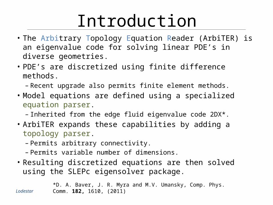
Introduction• The Arbitrary Topology Equation Reader (ArbiTER) is an

eigenvalue code for solving linear PDE’s in diverse geometries. • PDE’s are discretized using finite difference methods.

– Recent upgrade also permits finite element methods.• Model equations are defined using a specialized equation

parser. – Inherited from the edge fluid eigenvalue code 2DX*.

• ArbiTER expands these capabilities by adding a topology parser. – Permits arbitrary connectivity. – Permits variable number of dimensions.

• Resulting discretized equations are then solved using the SLEPc eigensolver package.

*D. A. Baver, J. R. Myra and M.V. Umansky, Comp. Phys. Comm. 182, 1610, (2011) Lodestar

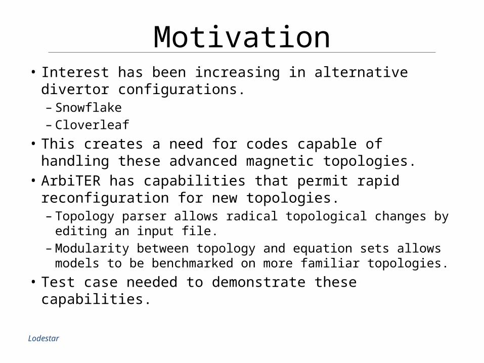
Motivation• Interest has been increasing in alternative divertor

configurations.– Snowflake– Cloverleaf

• This creates a need for codes capable of handling these advanced magnetic topologies.

• ArbiTER has capabilities that permit rapid reconfiguration for new topologies.– Topology parser allows radical topological changes by editing an

input file.– Modularity between topology and equation sets allows models to

be benchmarked on more familiar topologies.• Test case needed to demonstrate these capabilities.Lodestar

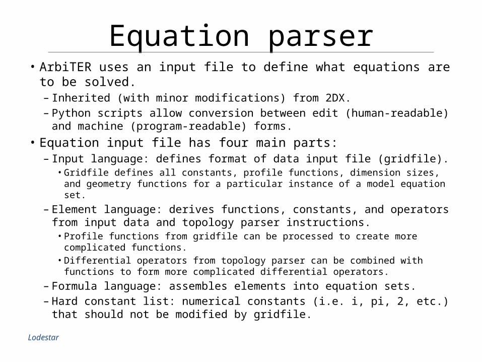
Equation parser• ArbiTER uses an input file to define what equations are to be solved.

– Inherited (with minor modifications) from 2DX.– Python scripts allow conversion between edit (human-readable) and

machine (program-readable) forms.• Equation input file has four main parts:

– Input language: defines format of data input file (gridfile).• Gridfile defines all constants, profile functions, dimension sizes, and geometry

functions for a particular instance of a model equation set.

– Element language: derives functions, constants, and operators from input data and topology parser instructions.• Profile functions from gridfile can be processed to create more complicated

functions.• Differential operators from topology parser can be combined with functions to form

more complicated differential operators.

– Formula language: assembles elements into equation sets.– Hard constant list: numerical constants (i.e. i, pi, 2, etc.) that should not be

modified by gridfile.Lodestar

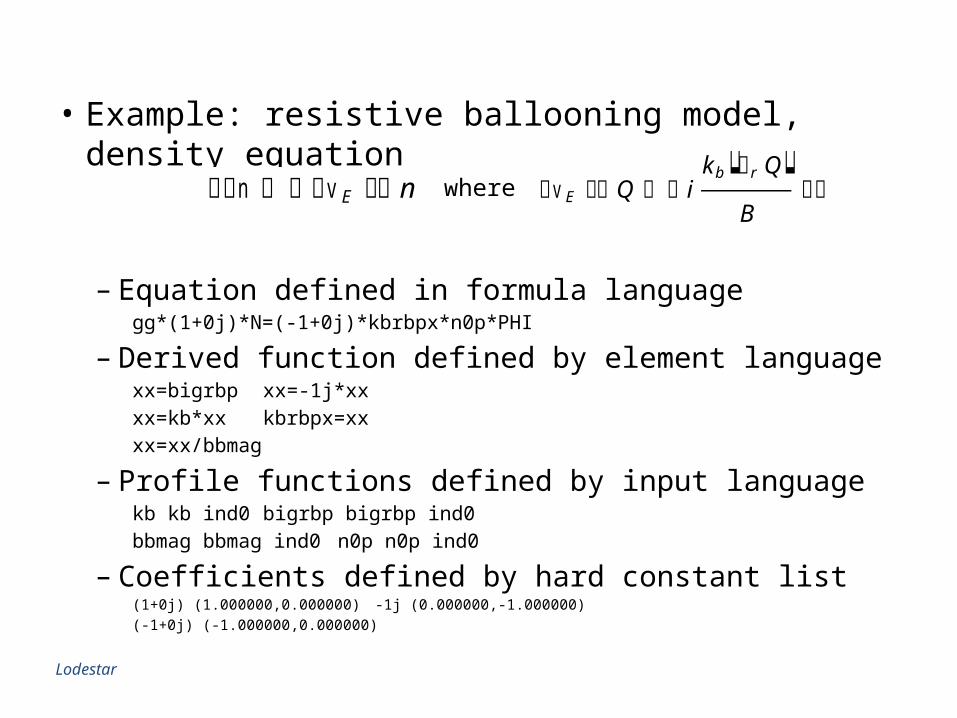
• Example: resistive ballooning model, density equation

– Equation defined in formula languagegg*(1+0j)*N=(-1+0j)*kbrbpx*n0p*PHI

– Derived function defined by element languagexx=bigrbp xx=-1j*xxxx=kb*xxkbrbpx=xxxx=xx/bbmag

– Profile functions defined by input languagekb kb ind0 bigrbp bigrbp ind0 bbmag bbmag ind0 n0p n0p ind0

– Coefficients defined by hard constant list(1+0j) (1.000000,0.000000) -1j (0.000000,-1.000000)(-1+0j) (-1.000000,0.000000)

n vE n vE Q ik b r Q

Bwhere

Lodestar

Topology parser• ArbiTER uses an input file to define the topology on which equations are to

be solved.– Python scripts allow conversion between edit (human-readable) and machine

(program-readable) forms. • Topology input file has two main parts:

– Integer language: processes integer inputs in order to calculate sizes of subregions.– Topology language: generates domains and operators for use in equation parser.

• Topology language creates four basic types of objects:– Bricks (blocks): simple meshes that can be arranged into more complicated

domains.– Domains: spaces on which a function or variable can be defined, created by

assembling bricks and linkages.– Linkages: sparse arrays relating points between two domains or bricks. Can be

used to define how bricks are assembled into domains, or can be used to construct operators.

– Operators: sparse arrays used to calculate derivatives, interpolation, etc. by the equation parser.

Lodestar

Example: 2DX emulation topology• Seven total bricks

– Edge, SOL, right private, left private– SOL and right private come in indented,

non-indented varieties– 1 x nx brick for periodic boundary condition

• Three domains– Indented (for staggered grids), non-indented,

and pbc• 24 linkages

– 9 for building domains– 15 for building operators

• PBC domain used to organize q function– q used to generate phase-shift periodic linkage

for the edge– every function must have a domain

• Remaining domains used to organize fields and functionsLodestar

Procedure• File containing magnetic geometry information in

UEDGE format imported to Mathematica.• Mathematica interacts with special version of

ArbiTER to import topology data.– Ensures that topology information is encapsulated in

topology parser language.– Allows Mathematica script to be used for multiple

topologies.• Mathematica script exports grid file to Arbiter.• Mathematica script reads Arbiter output for

processing and display.Lodestar

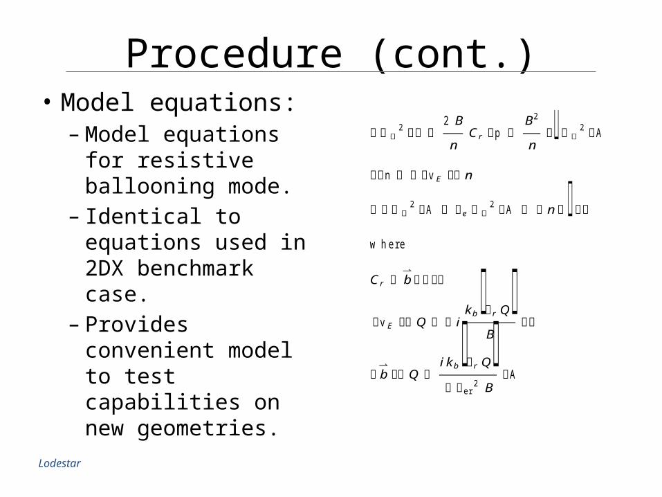
Procedure (cont.)• Model equations:– Model equations for

resistive ballooning mode.

– Identical to equations used in 2DX benchmark case.

– Provides convenient model to test capabilities on new geometries.

2

2 B

nC r p

B2

n

2 A

n vE n

2 A e

2 A n where

C r b

vE Q ik b r Q

B

b Q i k b r Q er 2 B

A

Lodestar

Results• Test case:– 30x80 resolution.– Temperature set to constant value (61.57 eV).– Density set to tanh function plus floor function.

• Scale length 16% of total flux width.• Peak density is 3x floor density.• Floor density is 1.4x1013 cm-3.

– Varying flux surface with peak density gradient allows control of dominant eigenmode position.

– Demonstrates interaction between eigenmode and features of given magnetic topology.

Lodestar

Results (cont.)|Phi| component of eigenfunctions as a function of density profile for n=20 (linear palette):

Lodestar

0 .995 1 .000 1 .005 1 .010

0 .5

1 .0

1 .5

2 .0

2 .5

3 .0n

0 .995 1 .000 1 .005 1 .010

0 .5

1 .0

1 .5

2 .0

2 .5

3 .0n

0 .995 1 .000 1 .005 1 .010

0 .5

1 .0

1 .5

2 .0

2 .5

3 .0n

0 .995 1 .000 1 .005 1 .010

0 .5

1 .0

1 .5

2 .0

2 .5

3 .0n

0 .995 1 .000 1 .005 1 .010

0 .5

1 .0

1 .5

2 .0

2 .5

3 .0n

Results (cont.)Close-up of case 4, log plot, 2x resolution

Lodestar

Results (cont.)Growth rate as a function of maximum gradient position,n=20

1 .000 1 .005 1 .010

4000

4500

5000

5500

6000

6500

s 1

Lodestar

Growth rate as a function of toroidal mode number, density profile from case 3

0 100 200 300 400n

50 000

100 000

150 000

200 000

s 1

Conclusions• ArbiTER is a linear solver capable of rapid

reconfiguration for new models and topologies.• The capabilities of this code have been

demonstrated on snowflake-minus topology with two x-points nearby in divertor region.

• Generality of code and modularity of physics models suggests other snowflake-related topologies can be modeled with little additional work.

Lodestar