Comput MechDOI 10.1007/s00466-017-1504-2

ORIGINAL PAPER

Modeling of power transmission and stress grading for coronaprotection

T. I. Zohdi1 · B. E. Abali1

Received: 1 July 2017 / Accepted: 26 October 2017© Springer-Verlag GmbH Germany, part of Springer Nature 2017

Abstract Electrical high voltage (HV) machines are proneto corona discharges leading to power losses as well as dam-age of the insulating layer. Many different techniques areapplied as corona protection and computational methods aidto select the best design. In this paper we develop a reduced-order model in 1D estimating electric field and temperaturedistribution of a conductor wrapped with different layers,as usual for HV-machines. Many assumptions and simpli-fications are undertaken for this 1D model, therefore, wecompare its results to a direct numerical simulation in 3Dquantitatively. Both models are transient and nonlinear, giv-ing a possibility to quickly estimate in 1D or fully computein 3D by a computational cost. Such tools enable understand-ing, evaluation, and optimization of corona shielding systemsfor multilayered coils.

Keywords Finite element · Electromagnetism · Coronaprotection · Temperature · Reduced order model

1 Introduction

With the invention of power transformer in 1880s, the feasi-bility of power transmission was greatly increased. Growingdemand in electric power motivates researchers for fur-ther optimization in power transmission. High voltage (HV)machines generate electric current transported in speciallydesigned cables as alternate current (AC) or direct current(DC). These HVAC or HVDC transmission mediums haveseveral inefficiencies leading to losses and leakage, which

B B. E. Abalibilenemek@abali.org

1 Department of Mechanical Engineering, University ofCalifornia, Berkeley, Berkeley, CA, USA

imply an active research and development, see [8,21,23].Two important issues for HVAC as well HVDC are: highamount of heat produced by the electric current and powerloss due to a corona discharge. These phenomena are alsorelated to each other, since the produced heat increasesthe temperature of the surrounding air, which enhances theionization leading to corona. The cables are insulated, forexample with resin like polypropylene or with a high-denseKraft paper, and along the surface of this insulation theelectric potential varies. If the potential gradient exceeds amaterial specific threshold value, coronas break down thesurface of insulating layer. Therefore, an extra layer is usedas corona protection by equalizing the potential gradient.

Coronaprotection is realizedbyusing apartially-insulatinglayer wrapped around the insulating layer surrounding theconducting core (copper). Silicon carbide filled resin orinorganic fiber reinforced composite material is used as asemiconductor around the insulator, see [7,17,18] and thereferences in [34]. Such a material is more efficient as a ther-mal conductor and also its electrical resistivity increases withan increasing applied electric field (voltage stress), E. Thiscorona protection layer can be applied as a lacquer (paint,spray) or tape (band). As outer corona protection or shield-ing (OCP or OCS), a slightly different coating is used than asend corona protection or shielding (ECP or ECS) along thewire. These different materials used for corona protection arecalled stress gradingmaterials—we use the wording electricfield instead of voltage stress. Such materials are semicon-ductors; hence, the resistivity depends on temperature aswellas on electric field, see [11,31].

Different proposals have been used for simulating the sys-tem response of power transmission. Maxwell’s equationscoupled with the balance of energy need to be solved in orderto obtain distribution of electromagnetic fields and temper-ature in the system. With system specific assumptions and

123

Comput Mech

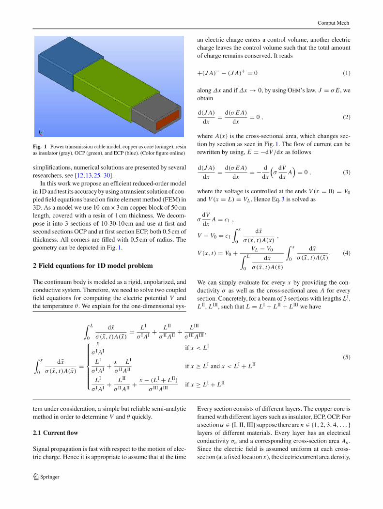
Fig. 1 Power transmission cable model, copper as core (orange), resinas insulator (gray), OCP (green), and ECP (blue). (Color figure online)

simplifications, numerical solutions are presented by severalresearchers, see [12,13,25–30].

In this work we propose an efficient reduced-order modelin 1Dand test its accuracybyusing a transient solutionof cou-pled field equations based on finite element method (FEM) in3D. As a model we use 10 cm×3cm copper block of 50cmlength, covered with a resin of 1cm thickness. We decom-pose it into 3 sections of 10-30-10cm and use at first andsecond sections OCP and at first section ECP, both 0.5cm ofthickness. All corners are filled with 0.5cm of radius. Thegeometry can be depicted in Fig. 1.

2 Field equations for 1D model problem

The continuum body is modeled as a rigid, unpolarized, andconductive system. Therefore, we need to solve two coupledfield equations for computing the electric potential V andthe temperature θ . We explain for the one-dimensional sys-

tem under consideration, a simple but reliable semi-analyticmethod in order to determine V and θ quickly.

2.1 Current flow

Signal propagation is fast with respect to the motion of elec-tric charge. Hence it is appropriate to assume that at the time

an electric charge enters a control volume, another electriccharge leaves the control volume such that the total amountof charge remains conserved. It reads

+(J A)− − (J A)+ = 0 (1)

along Δx and if Δx → 0, by using Ohm’s law, J = σ E , weobtain

d(J A)

dx= d(σ E A)

dx= 0 , (2)

where A(x) is the cross-sectional area, which changes sec-tion by section as seen in Fig. 1. The flow of current can berewritten by using, E = −dV/dx as follows

d(J A)

dx= d(σ E A)

dx= − d

dx

(σdV

dxA)

= 0 , (3)

where the voltage is controlled at the ends V (x = 0) = V0and V (x = L) = VL . Hence Eq.3 is solved as

σdV

dxA = c1 ,

V − V0 = c1

∫ x

0

dx̄

σ(x̄, t)A(x̄),

V (x, t) = V0 + VL − V0∫ L

0

dx̄

σ(x̄, t)A(x̄)

∫ x

0

dx̄

σ(x̄, t)A(x̄). (4)

We can simply evaluate for every x by providing the con-ductivity σ as well as the cross-sectional area A for everysection. Concretely, for a beam of 3 sections with lengths L I,L II, L III, such that L = L I + L II + L III we have

∫ L

0

dx̄

σ(x̄, t)A(x̄)= L I

σ IAI + L II

σ IIAII + L III

σ IIIAIII ,

∫ x

0

dx̄

σ(x̄, t)A(x̄)=

⎧⎪⎪⎪⎪⎪⎪⎨⎪⎪⎪⎪⎪⎪⎩

x

σ IAI if x < L I

L I

σ IAI + x − L I

σ IIAII if x ≥ L I and x < L I + L II

L I

σ IAI + L II

σ IIAII + x − (L I + L II)

σ IIIAIII if x ≥ L I + L II

(5)

Every section consists of different layers. The copper core isframed with different layers such as insulator, ECP, OCP. Fora sectionα ∈ {I, II, III} suppose there aren ∈ {1, 2, 3, 4, . . . }layers of different materials. Every layer has an electricalconductivity σn and a corresponding cross-section area An .Since the electric field is assumed uniform at each cross-section (at a fixed location x), the electric current area density,

123

Comput Mech

σ(x, t)E , over the whole cross-section reads

1

A(x)

∫

A(x)J dA = 1

A(x)

n∑i=1

Ji Ai = 1

A(x)

n∑i=1

σi E Ai .

(6)

Thus, we obtain

σ(x, t) = 1

A(x)

n∑i=1

σi Ai . (7)

The effective conductivity of a cross-section is the sum ofthe individual conductivities multiplied by their share of thecross-sectional area. In each section we have

σα = 1

Aα

n∑i=1

σαi Aα

i , Aα =n∑

i=1

Aαi . (8)

In each section, the number of layers may vary, n = n(α),which we have omitted in the notation for the sake of brevity.

2.2 Temperature evolution

Analogously,we use the energy conservationwithin a controlvolume

ρc∂θ

∂tΔV = +(q A)− − (q A)+ + aJ EΔV , (9)

where the volume is ΔV = AΔx , c denotes the (constantin each section) specific heat capacity, q = −κ∂θ/∂x is theheat flux, and a system specific parameter a models possiblelosses from the control volume, we set a = 1. Dividing bothsides by ρcΔV yields

∂θ

∂t= 1

ρc

∂

∂x

(κ

∂θ

∂x

)+ J E

ρc︸ ︷︷ ︸F(x, t)

. (10)

Approximating the time derivative of θ at x and t as

∂θ

∂t≈ θ(x, t + Δt) − θ(x, t)

Δt(11)

we obtain

θ(x, t + Δt) = θ(x, t) + ΔtF(x, t) . (12)

For the derivative term inside of F, we approximate

∂

∂x

(κ

∂θ

∂x

)= ∂

∂x

(κ(x)

Δx

(θ(x + Δx

2

)− θ

(x − Δx

2

)))

= 1

(Δx)2

(κ(x + Δx

2

)(θ(x + Δx) − θ(x)

)

− κ(x − Δx

2

)(θ(x) − θ(x − Δx)

)). (13)

2.3 Algorithm

The solution algorithm for the reduced-order model worksin 1D. The geometry consists of different parts (layers) suchas copper, resin, ECP, and OCP. These layers have differentmaterial properties used for calculating the effective con-ductivity. In the 1D model we compute electric potential andtemperature onlywithin the copper core; however,we presentthe results on a 3Dmesh for the sake of a better visualization.

A line mesh is generated and along that line the electricpotential is computed with Eq. (4) by using the temperaturefield from the last time step. Since we have neglected polar-ization, the electric potential is identical for different layers.Therefore, we can solve for the whole body with one reduced1Dmodel. After the computation of the electric potential, thetemperature distribution is computed with Eq. (12) by usingthe current electric potential. Since Joule’s heat depends onthe material coefficient (electrical conductivity), for each ofthe layer we need to determine the temperature separatelyas another 1D model. So in each time step we follow thesteps:

– Compute the electric potential V along x by using thetemperature from the last time step θ0 (or initial condi-tion),

– Compute J and E with the current value of σ in eachlayer,

– Compute θ(x, t + Δt) at each node in system,– Compute σ ∗(x, t + Δt), go to the next time step and

repeat.

We solve two 1D equations: one for electric potential andanother for temperature. Then we derive electric field andelectric current from the solution and combine them in a 3Dmesh for a better visualization. The computation is fast; butit may be error prone effected by the various assumptions.First,we assume rigid bodies andneglect dielectric propertiesof the materials (no polarization). Second, we use a weakcoupling in the sense that the temperature and the electricfield affect each other with a delay of one time step. Third,we neglect the magnetic potential completely. Fourth, theheat flux is only along x1 and we ignore a heat exchange withthe environment (no losses). These assumptionsmight lead toinaccuracies. In order to estimate the accuracy of this reducedmodel, we implement a direct numerical computation in 3Dand compare the results of 1D to the results in 3D.

123

Comput Mech

3 Direct numerical FEM calculations

Consider a rigid, polarized continuum body, within whichwe want to compute the electric potential φ, the magneticpotential A, and the temperature T as a function in spacex and in time t . We call the list unknowns {φ, A, T } as theprimitive variables. The solution of primitive variables hasto fulfill the governing equations motivated by balance equa-tions. We very briefly sum up this motivation and presentthe governing equations, for details we refer to [2, Chap. 3].All fields are expressed in Cartesian coordinates, we applyEinstein’s summation convention over repeated indices, andwe understand a derivative with respect to xi by the commanotation (·),i as a lower index.

The continuum body has an electric charge composed offree and bound charges. Their characteristics differ since thefree charges move in macroscopic distances, whereas thebound charges displace in microscopic lengths.We start withthe balance of electric charge as well as balance of magneticflux such that four Maxwell equations are derived. Two ofthem can be solved by means of the following ansatz func-tions

Ei = −φ,i − ∂Ai

∂t, Bi = εi jk Ak, j , (14)

between electromagnetic fields Ei , Bi and electromagneticpotentials φ, Ai up to an arbitrary gauge—because of numer-ical reasons,we apply theLorenz gauge.By startingwith thebalance of electric charge and inserting Maxwell’s equa-tions, we obtain

∂Di,i

∂t+

(J fr.i + εi jkMk, j

),i

= 0 , (15)

where the charge potentialDi (also called the dielectric dis-placement) is created by the free electric charges, J fr.i denotesthe electric current due to the motion of the free electriccharges, εi jk is the Levi- Civita symbol being equal to thepermutation symbol in Cartesian coordinates, and the mag-netic polarization Mi is the magnetization effected by thebound electric charges. In the case of a rigid body, for Di ,J fr.i , and Mi we apply following constitutive equations:

Di = Di + Pi , Di = ε0Ei , Pi = ε0χel.Ei ,

J fr.i = σπT,i + σ Ei , Mi = χmag.

μ0(1 + χmag.)Bi , (16)

giving the connection to the electric field Ei , the magneticflux Bi , and the temperature T by means of the universalconstants ε0 and μ0, as well as the material specific coeffi-cients, namely the electrical conductivity σ , thermoelectricor Peltier’s constantπ , electric susceptibilityχel., andmag-netic susceptibility χmag.. Electric polarization Pi is due to

the bound electric charges. Herein we neglect the magneto-electric effect such that electric polarization depends only onthe electric field, analogously,magnetic polarization dependsonly on themagnetic flux. For computing themagnetic poten-tial, Ai , we utilize Maxwell’s equation and after insertingthe Lorenz gauge, we acquire

ε0∂2Ai

∂t2− 1

μ0Ai, j j = J fr.i + ∂Pi

∂t+ εi jkMk, j . (17)

For computing the temperature T , we use the balance ofentropy

ρ∂η

∂t+ Φi,i − ρ

r

T= Σ , (18)

where the supply term r vanishes in our application, the spe-cific (per mass) entropy η and its flux Φi as constitutiveequations and the production term Σ read

η = c ln( T

Tref.

), Φi = qi

T, qi = −κT,i + σπT Ei ,

Σ = − qiT 2 T,i + 1

TEi J

fr.i , (19)

for rigid, polarized, thermal bodies under the assumptionthat irreversible polarization effects (such as hysteresis)are neglected. The additional material coefficients—specificheat capacity c, thermal conductivity κ—need to be deter-mined for every different material by means of experiments.

The governing Eqs. (15), (17), (18) are coupled and non-linear. In order to solve them we use finite element methodin space and finite difference method in time. For thespace discretization we follow the standard variational for-mulation, namely multiply the governing equations withappropriate test functions and integrate by parts for weak-ening the continuity condition. The 5 primitive variablesp = {φ, A1, A2, A3, T } are approximated as a classCn func-tion in 5-dimensional Hilbert space,

V ={p ∈ [Hn(Ω)]5 : p

∣∣∂Ω

= given}

, (20)

where the differentiability properties are included such thatit is a Sobolev space. For the sake of simplicity, we omit toemphasize the discrete representations of the analytic func-tions and use the same symbols henceforth. Furthermore,we use the Galerkin approach and choose test functionsfrom the same space as the primitive variables, whereas thetest functions vanish on the Dirichlet boundaries. For thetime discretization,we choose theEuler backwards schema.After space and time discretization, we acquire the followingweak forms:

Fφ =∫

Ω

(−(Di − D0

i )δφ,i − Δt J fr.i δφ,i −Δtεi jkMk, j δφ,i

)dv

123

Comput Mech

+∫

∂ΩniΔtεi jk�Mk, j �δφda,

FA =∫

Ω

(ε0

Ai − 2A0i + A00

Δt2δAi + 1

μ0Ai, j δAi, j − J fr.i δAi

− Pi − P0i

ΔtδAi + εi jkMkδAi, j

)dv,

FT =∫

Ω

(ρ(η − η0)δT−ΔtΦi δT,i − Δtρ

r

TδT−ΔtΣδT

)dv

+∫

∂ΩΔt�Φi �δTnida. (21)

We solve in discrete time steps. Termswith an upper indexof zero, (·)0, denote the numerical values from the last timestep. The jump brackets, �(·)�, indicate the difference on asurface between the values determined by the shape func-tions of adjacent (neighboring) finite elements. The solutionfields, namely φ, Ai , and T are continuous over the elementboundaries; however, the constitutive equations may havejumps across the interface between two different materials.We already applied the well-known jump conditions overthe element boundaries by assuming that no surface chargesand currents are existing and assuming that the electric cur-rent is continuous (along the normal direction ni ), see [4] fordetails. Assembly over the whole domain give the nonlinearand coupled weak form

Form = Fφ + FA + FT , (22)

which is solved after an automatic linearization at the partialdifferential level by using the novel collection of packagesdeveloped under the FEniCS project [16,20]. It is importantto distinguish the method used herein from the rich literaturefor computation of electromagnetism. We use standard finiteelements of order one, which is not used for electromag-netism. Starting with [24] and [22], solution of Maxwell’sequation are obtained by using mixed elements, for differ-ent proposals and implementations, see [6,9], [10, Sect. 17],[14,19]. Nowadays, there exist several element types, see [5].Roughly, the overall idea relies on solving electromagneticfields, Ei and Bi , by satisfying all Maxwell equations. Ofcourse, this strategy is fine; however, by using electromag-netic potentials, φ and Ai , it is possible to solve the systemby means of standard finite elements, as presented in [2,Chap. 3], [3,4] with various examples. We use the same ele-ment type, namely P1 continuous Lagrange elements oforder one for each primitive variable.

4 Material properties

As electrical conductor, nearly always, copper is used, whichis a homogeneous and isotropic material at least in the mil-limeter length-scale. The copper core is surrounded by an

insulator in order to avoid arcing. A polymeric type of resinwill be modeled. ECP and OCP are particle-functionalizedor fiber reinforced composite materials. Owing to the natureof composite character, we need to introduce estimates onthe material properties. For every constitutive equation forOCP and ECP, we use “effective” material constants

〈Pi 〉Ω = ε0χ∗el.〈Ei 〉Ω ,

〈Mi 〉Ω = χmag.

μ0(1 + χ∗mag.)

〈Bi 〉Ω ,

〈J fr.i 〉Ω = −σ ∗π∗〈T,i 〉Ω + σ ∗〈Ei 〉Ω ,

〈qi 〉Ω = −κ∗〈T,i 〉Ω + σ ∗π∗〈T 〉Ω 〈Ei 〉Ω , (23)

where (·)∗ is the effective material parameter of the com-posite material, 〈·〉Ω is the volume averaged field with theaveraging operator:

〈·〉Ω def= 1

|Ω|∫

Ω

(·)dΩ (24)

over a statistically representative volume element withdomain Ω . In the following we briefly present how to esti-mate the effective parameters based on [32,33].

4.1 Determining the effective material parameters

In order to make estimates of the overall properties ofthe composite, we consider the widely used Hashin–Shtrikman bounds for isotropic materials with isotropiceffective responses. These estimates provide one with upperand lower bounds on the overall response of the material. Fortwo isotropicmaterials with an overall isotropic response, weutilize the following estimates:

σ1 + v21

σ2−σ1+ 1−v2

3σ1︸ ︷︷ ︸σ ∗,−

≤ σ ∗ ≤ σ2 + 1 − v21

σ1−σ2+ v2

3σ2︸ ︷︷ ︸σ ∗,+

, (25)

where the conductivity of phase 2 (with volume fraction v2) islarger than phase 1 (σ2 ≥ σ1). Usually, v2 corresponds to theparticle material, although there can be applications wherethe matrix is more conductive than the particles. In that case,v2 would correspond to the matrix material. Provided thatthe volume fractions and constituent conductivities are theonly known information about themicrostructure, the expres-sions are the tightest bounds for the overall isotropic effectiveresponses for two phase media, where the constituents areboth isotropic. A critical observation is that the lower boundis more accurate when the material is composed of high con-ductivity particles that are surrounded by a low conductivitymatrix (denoted case 1) and the upper bound ismore accurate

123

Comput Mech

for a high conductivity matrix surrounding low conductivityparticles (denoted case 2).

This can be explained by considering two cases ofmaterialcombinations, one with 50% low conductivity material and50% high conductivity material. A material with a continu-ous low conductivity (fine-scale powder) binder (50%) willisolate the high conductivity particles ((50%), and the overallsystem will not conduct electricity well (this is case 1 andthe lower bound is more accurate), while a material formedby a continuous high conductivity (fine-scale powder) binder(50%) surrounding low conductivity particles (50%, case 2)will, in an overall sense, conduct electricity better than case1. Thus, case 2 is more closely approximated by the upperbound and case 1 is closer to the lower bound. Since the trueeffective property lies between the upper and lower bounds,one can construct the following approximation

σ ∗ ≈ Ψ σ ∗,+ + (1 − Ψ )σ ∗,−, (26)

where 0 ≤ Ψ ≤ 1 depends on themicrostructure andmust becalibrated. For high conductivity spherical particles, at lowvolume fractions, under 15%, where the particles are not incontact, the lower bound is more accurate. Thus, one wouldpick Ψ = Ψ s ≤ 0.5 to bias the estimate to the lower bound.However, using the same setup but replacing the sphericalparticles with flakes, there is a greater likelihood of connect-ing flakes, thus producing high-conductivity pathways. Theiroverall conductivity will be higher than those of sphere at thesame volume fraction. Thus, onewould pickΨ = Ψ f > Ψ s .One can calibrateΨ by comparing it to different experimentsas already done in [35]. Essentially, more particle interactionmakes the upper bound more relevant. The general trends are(a) for cases where the upper bound is more accurate,Ψ > 1

2and (b) for cases when the lower bound is more accurate,Ψ < 1

2 . The parameter Ψ indicates the degree of interac-tion of the particulate constituents. Analogously, the thermalconductivity has the following bounds

κ1 + v21

κ2−κ1+ 1−v2

3κ1︸ ︷︷ ︸κ∗,−

≤ κ∗ ≤ κ2 + 1 − v21

κ1−κ2+ v2

3κ2︸ ︷︷ ︸κ∗,+

. (27)

such that the effective parameter reads

κ∗ ≈ Ψ κ∗,+ + (1 − Ψ )κ∗,− . (28)

In case of other material specific parameters, namely themass density, the heat capacity, the susceptibilities, we usethe volumetric fraction such that the microstructure effect isexcluded

ρ∗ = (1 − v2)ρ1 + v2ρ2 ,

<1/2 >1/2ΨΨ

PARTICLES WELL SEPARATED PARTICLE TOUCHING

Fig. 2 Comparing microstructures with the same volume fractions.Flakes touch more, and thus need a higher value of Ψ

c∗ = (1 − v2)c1 + v2c2 ,

χ∗ = (1 − v2)χ1 + v2χ2. (29)

4.2 Nonlinearity due to the material parameters

As pointed out in the Introduction, the heat and electricalconductive material properties of all the materials depend ontemperature and electric field.Weassume for this dependencethe following functional form:

σ = σo exp(

− C1T − Tref.Tref.

)exp

(− C2

‖E‖ − Eref.

Eref.

),

κ = κo exp(

− C3T − Tref.Tref.

)exp

(− C4

‖E‖ − Eref.

Eref.

),

(30)

where C× are material constants and Tref., Eref. are refer-ence values. For Tref. we can choose the initial temperature,where no flux or stress arise. For Eref. we can choose theelectric field at the breakdown voltage, at which the insula-tor becomes partially conductive. The constant σo, κo is thevalue at the reference temperature and electric field. For thesake of simplicity we will use C3 = C4 = 0 providing aconstant thermal conductivity.

5 Results and comparison

By using the reduced model and FEM implementation, wesolve the system shown in Fig. 1 out of four different mate-rials for the equal set of boundary conditions. Since theconductivity of copper is high, there is a significant amountof production of entropy due to Joule’s loss, increasing thetemperature of the system (Fig. 2). For the reduced model weonly solve in 1D and visualize in 3D by using the materialcoefficients compiled in Table 1.

In the case of FEM implementation, we embed the geom-etry in air as shown in Fig. 3.

123

Comput Mech

Table 1 Material coefficients for the reduced model

Material Coefficient Unit

Copper ρ = 8960 kg/m3

σo = 5.8 · 107 S/m

C1 = 1 –

C2 = 0 –

κ = 400 W/(mK)

c = 390 J/(kgK)

Epoxy resin ρ = 1000 kg/m3

σo = 1 · 10−13 S/m

C1 = 0 –

C2 = 10 –

κ = 1.5 W/(mK)

c = 800 J/(kgK)

Eref. = 500 · 106 V/m

OCP ρ∗ = 1100 kg/m3

σ ∗o = 10 S/m

C1 = 10 –

C2 = 10 –

κ∗ = 1 W/(mK)

c∗ = 1000 J/(kgK)

Eref. = 20 · 106 V/m

ECP ρ∗ = 3000 kg/m3

σ ∗o = 103 S/m

C1 = 10 –

C2 = 0 –

κ∗ = 10 W/(mK)

c∗ = 700 J/(kgK)

Fig. 3 Power transmission cable model, copper as core (orange), resinas insulator (gray), OCP (green), and ECP (blue), all embedded in air(transparent). (Color figure online)

This 3D geometry allows us to set homogeneous farfield boundaries, i.e., electromagnetic potentials vanish at

Table 2 Additional material coefficients for the FEM model

Material Coefficient Unit

Copper χel. = 0 –

χmag. = −1 · 10−5 –

π = 68 · 10−6 V/K

Resin χel. = 2 –

χmag. = 0 –

π = 0 V/K

OCP χ∗el. = 5 –

χ∗mag. = 0 –

π∗ = 0 V/K

ECP χ∗el. = 10 –

χ∗mag. = 0 –

π∗ = 0 V/K

Air ρ = 1.2 kg/m3

σo = 3 · 10−15 S/m

C1 = 0 –

C2 = 0 –

κ = 0.0257 W/(mK)

c = 1005 J/(kgK)

χel. = 0 –

χmag. = 0 –

π = 0 V/K

the outer shell. In addition to Table 1, we use the materialparameters from Table 2.

All material constants are approximate but realistic val-ues. The intention in this work is to test the proposed 1Dmodel against 3D model quantitatively. In the 1D approachwe obtain quick results because of several simplifications.One time step lasts approximately 1.5 s on a single core,1

where most of the computation time is used for projectingon a 3D mesh for the sake of a better visualization. In the 3Dmodel we involve many coupling effects and assume that theresult ismore accurate than the 1Dapproach.As expected, 3Dmodeling takes longer, for a time step approximately 17minon 6 cores with the samemachine.We perform a test examplewith both approaches and compare them in the following.

Consider a power station of P = 0.5MW where at thebeginning of transmission the electric potential is convertedto (a relatively low potential difference) V = 30kV at a stan-dard frequency of 50Hz. The conductor copper possessesthe resistance R = V 2/P and the resistivity r = RA/L ,where the cross-section A = AI and the total length L =L I+L II+L III are given. The electrical conductivity of copperis exchanged with σo = 1/r in order to model this phe-nomenon. In reality, there is an additional resistor restricting

1 Intel Core i7-2600 at 3.4GHz running on Ubuntu server with Linux4.4.0-64-generic

123

Comput Mech

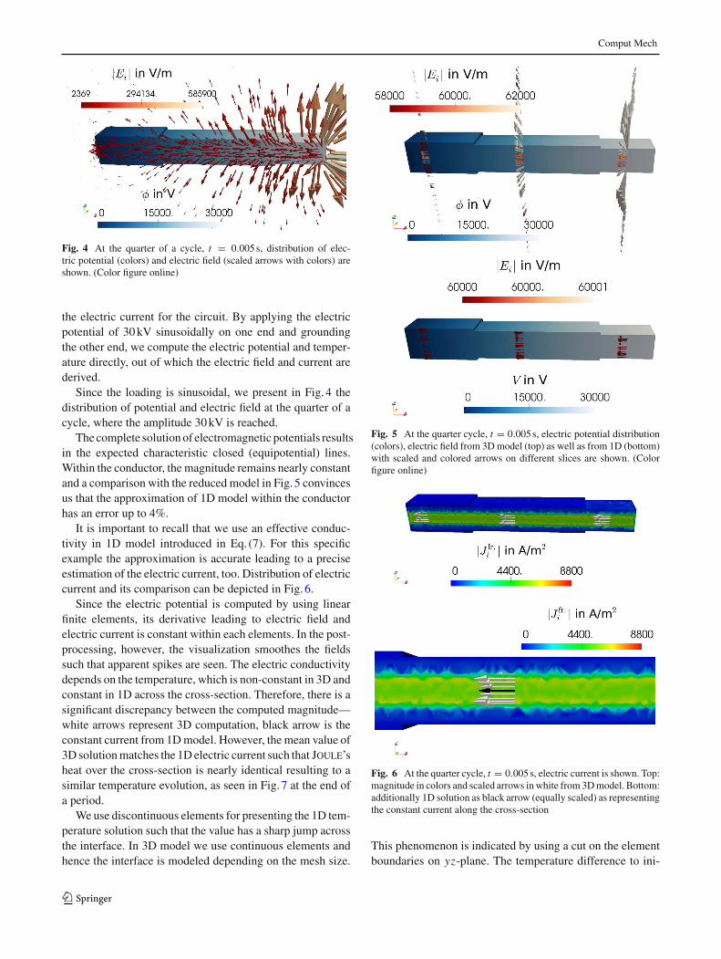
Fig. 4 At the quarter of a cycle, t = 0.005s, distribution of elec-tric potential (colors) and electric field (scaled arrows with colors) areshown. (Color figure online)

the electric current for the circuit. By applying the electricpotential of 30kV sinusoidally on one end and groundingthe other end, we compute the electric potential and temper-ature directly, out of which the electric field and current arederived.

Since the loading is sinusoidal, we present in Fig. 4 thedistribution of potential and electric field at the quarter of acycle, where the amplitude 30kV is reached.

The complete solutionof electromagnetic potentials resultsin the expected characteristic closed (equipotential) lines.Within the conductor, the magnitude remains nearly constantand a comparison with the reduced model in Fig. 5 convincesus that the approximation of 1D model within the conductorhas an error up to 4%.

It is important to recall that we use an effective conduc-tivity in 1D model introduced in Eq. (7). For this specificexample the approximation is accurate leading to a preciseestimation of the electric current, too. Distribution of electriccurrent and its comparison can be depicted in Fig. 6.

Since the electric potential is computed by using linearfinite elements, its derivative leading to electric field andelectric current is constant within each elements. In the post-processing, however, the visualization smoothes the fieldssuch that apparent spikes are seen. The electric conductivitydepends on the temperature, which is non-constant in 3D andconstant in 1D across the cross-section. Therefore, there is asignificant discrepancy between the computed magnitude—white arrows represent 3D computation, black arrow is theconstant current from 1Dmodel. However, the mean value of3D solutionmatches the 1D electric current such that Joule’sheat over the cross-section is nearly identical resulting to asimilar temperature evolution, as seen in Fig. 7 at the end ofa period.

We use discontinuous elements for presenting the 1D tem-perature solution such that the value has a sharp jump acrossthe interface. In 3D model we use continuous elements andhence the interface is modeled depending on the mesh size.

Fig. 5 At the quarter cycle, t = 0.005s, electric potential distribution(colors), electric field from 3Dmodel (top) as well as from 1D (bottom)with scaled and colored arrows on different slices are shown. (Colorfigure online)

Fig. 6 At the quarter cycle, t = 0.005s, electric current is shown. Top:magnitude in colors and scaled arrows inwhite from 3Dmodel. Bottom:additionally 1D solution as black arrow (equally scaled) as representingthe constant current along the cross-section

This phenomenon is indicated by using a cut on the elementboundaries on yz-plane. The temperature difference to ini-

123

Comput Mech

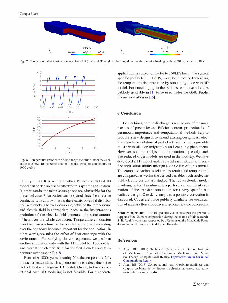
Fig. 7 Temperature distribution obtained from 1D (left) and 3D (right) solutions, shown at the end of a loading cycle at 50Hz, i.e., t = 0.02 s

−6

−4

−2

0

2

4

6×104

Ein

V/m

0.00 0.02 0.04 0.06 0.08 0.10 0.12t in s

300350400450500550600650700750

Tin

K

0 5 10 15 20t in s

Fig. 8 Temperature and electric field change over time under the exci-tation at 50Hz. Top: electric field in 5 cycles. Bottom: temperature in1000 cycles

tial Tref. = 300K is accurate within 1% error such that 1Dmodel can be declared as verified for this specific application.In other words, the taken assumptions are admissible for thepresented case. Polarization can be spared since the effectiveconductivity is approximating the electric potential distribu-tion accurately. The weak coupling between the temperatureand electric field is appropriate, because the instantaneousevolution of the electric field generates the same amountof heat over the whole conductor. Temperature conductionover the cross-section can be omitted as long as the coolingover the boundary becomes important for the application. Inother words, we miss the effect of heat exchange with theenvironment. For studying the consequences, we performanother simulation only with the 1D model for 1000 cyclesand present the electric field for the first 5 cycles and tem-perature over time in Fig. 8.

Even after 1000 cycles meaning 20s, the temperature failsto reach a steady state. This phenomenon is indeed due to thelack of heat exchange in 1D model. Owing to the compu-tational cost, 3D modeling is not feasible. For a concrete

application, a correction factor to Joule’s heat—the systemspecific parameter a in Eq. (9)—can be introduced amendingthe temperature rise over time by simulating once with 3Dmodel. For encouraging further studies, we make all codespublicly available in [1] to be used under the GNU Publiclicense as written in [15].

6 Conclusion

In HVmachines, corona discharge is seen as one of the mainreasons of power losses. Efficient corona protection is ofparamount importance and computational methods help topropose a new design or to amend existing designs. An elec-tromagnetic simulation of part of a transmission is possiblein 3D with all electrodynamics and coupling phenomena.However, such an analysis is computationally costly suchthat reduced-order models are used in the industry. We havedeveloped a 1D model under several assumptions and veri-fied their admissibility through a single run of a 3D model.The computed variables (electric potential and temperature)are compared, as well as the derived variables such as electricfield, electric current are studied. The reduced-order modelinvolving material nonlinearities performs an excellent esti-mation of the transient simulation for a very specific butrealistic design. One deficiency and a possible correction isdiscussed. Codes are made publicly available for continua-tion of similar efforts for concrete geometries and conditions.

Acknowledgements T. Zohdi gratefully acknowledges the generoussupport of the Siemens corporation during the course of this research.B. E. Abali’s work was supported by a Grant from the Max Kade Foun-dation to the University of California, Berkeley.

References

1. Abali BE (2016) Technical University of Berlin, Instituteof Mechanics, Chair of Continuum Mechanics and Mate-rial Theory, Computational Reality. http://www.lkm.tu-berlin.de/ComputationalReality

2. Abali BE (2017) Computational reality, solving nonlinear andcoupled problems in continuum mechanics. advanced structuredmaterials. Springer, Berlin

123

Comput Mech

3. Abali BE (2017) Computational study for reliability improvementof a circuit board. Mech Adv Mater Mod Processes 3(1):11

4. Abali BE, Reich FA (2017) Thermodynamically consistent deriva-tion and computation of electro-thermo-mechanical systems forsolid bodies. Comput Methods Appl Mech Eng 319:567–595

5. Arnold DN, Logg A (2014) Periodic table of the finite elements.SIAM News 47(9):212

6. Bossavit A (1988) Whitney forms: a class of finite elements forthree-dimensional computations in electromagnetism. In: IEEEProceedings a physical science, measurement and instrumentation,management and education, reviews, 135(8):493–500

7. BrockschmidtM,Gröppel P, Pohlmann F, RohrC,RödingR (2013)Material for insulation system, insulation system, external coronashield and an electric machine, February 20 2013. US Patent App.14/386,261

8. Chen G, Hao M, Xu Z, Vaughan A, Cao J, Wang H (2015) Reviewof high voltage direct current cables. CSEE J Power Energy Syst1(2):9–21

9. Ciarlet P Jr, Zou J (1999) Fully discrete finite element approachesfor time-dependent maxwell’s equations. Numerische Mathematik82(2):193–219

10. Demkowicz L (2006) Computing with hp-adaptive finite elements:volume 1 one and two dimensional elliptic andMaxwell problems.CRC Press, Boca Raton

11. Donzel L, Greuter F, Christen T (2011) Nonlinear resistive electricfield grading part 2: materials and applications. IEEE Electr InsulMag 27(2):18–29

12. Egiziano L, Tucci V, Petrarca C, Vitelli M (1999) A galerkin modelto study the field distribution in electrical components employingnonlinear stress gradingmaterials. IEEETransDielectr Electr Insul6(6):765–773

13. Gatzsche M, Lücke N, Großmann S, Kufner T, Freudiger G (2017)Evaluation of electric-thermal performance of high-power contactsystems with the voltage-temperature relation. IEEE Trans Com-pon Packag Manuf Technol 7(3):317–328

14. Gillette A, Rand A, Bajaj C (2016) Construction of scalar andvector finite element families on polygonal and polyhedral meshes.Comput Methods Appl Math 16(4):667–683

15. GNU Public. Gnu general public license. http://www.gnu.org/copyleft/gpl.html, June 2007

16. Hoffman J, Jansson J, Johnson C, Knepley M, Kirby RC, Logg A,Scott LR, Wells GN (2005) FEniCS. http://www.fenicsproject.org

17. Kelen A, Virsberg L-G (1962) Coating for equalizing the potentialgradient along the surface of an electric insulation, November 271962. US Patent 3,066,180

18. Klaussner B, Meyer C, Muhrer V, Maurer A, Russel C, SchaferK (2004) Corona shield, and method of making a corona shield,December 16 2004. US Patent App. 11/014,631

19. Li J (2009) Numerical convergence and physical fidelity analysisfor maxwell’s equations in metamaterials. Comput Methods ApplMech Eng 198(37):3161–3172

20. Logg A, Mardal KA, Wells GN (2011) Automated solution of dif-ferential equations by the finite element method, the FEniCS book,lecture notes in computational science and engineering, vol 84.Springer, Berlin

21. Meah K, Ula S (2007) Comparative evaluation of hvdc and hvactransmission systems. In: Power engineering society general meet-ing, 2007. IEEE, pp 1–5

22. Nédélec J-C (1980)Mixedfinite elements inR3.NumerischeMath-ematik 35(3):315–341

23. Planas E, Andreu J, Gárate JI, de Alegría IM, Ibarra E (2015) ACand DC technology in microgrids: a review. Renew Sustain EnergyRev 43:726–749

24. Raviart P-A, Thomas J-M (1977) A mixed finite element methodfor 2-nd order elliptic problems. In: Mathematical aspects of finiteelement methods. Springer, pp 292–315

25. Schmidt G, Litinsky A, Staubach A (2015) Enhanced calcula-tion and dimensioning of outer corona protection systems in largerotating machines. In: International symposium on high voltageengineering

26. Sharifi E, Jayaram S, Cherney EA (2010) A coupled electro-thermal study of the stress grading system of medium voltagemotor coils when energized by repetitive fast pulses. In: Confer-ence record of the 2010 IEEE international symposiumon electricalinsulation (ISEI)

27. Sima W, Espino-Cortes FP, Cherney EA, Jayaram SH (2004)Optimization of corona ring design for long-rod insulators usingfem based computational analysis. In: Conference record of the2004 IEEE international symposium on electrical insulation, 2004.IEEE, pp 480–483

28. Staubach C, Wulff J, Jenau F (2012) Particle swarm based simplexoptimization implemented in a nonlinear, multiple-coupled finite-element-model for stress grading in generator end windings. In:2012 13th international conference on optimization of electricaland electronic equipment (OPTIM). IEEE, pp 482–488

29. Stefanini D, Seifert JM, ClemensM,Weida D (2010) Three dimen-sional fem electrical field calculations for EHVcomposite insulatorstrings. In: 2010 IEEE international powermodulator and high volt-age conference (IPMHVC). IEEE, pp 238–242

30. WeidaD,Böhmelt S,ClemensM(2010)DesignofZnOmicrovaris-tor end corona protection for electrical machines. In: Conferencerecord of the 2010 IEEE international symposium on electricalinsulation (ISEI). IEEE, pp 1–4

31. Wheeler JCG, Gully AM, Baker AE, Perrot FA (2007) Thermalperformance of stress grading systems for converter-fed motors.IEEE Electr Insul Mag 23(2):5–11

32. Zohdi TI (2012) Electromagnetic properties of multiphasedielectrics: a primer on modeling, theory and computation, vol 64.Springer, Berlin

33. Zohdi TI, Wriggers P (2008) An introduction to computationalmicromechanics, 2nd edn. Springer, Berlin

34. Zohdi TI (2017) Modeling and rapid simulation of the propagationand multiple branching of electrical discharges in gaseous atmo-spheres. Comput Mech 60(3):433–443

35. Zohdi TI, Monteiro PJM, Lamour V (2002) Extraction of elasticmoduli from granular compacts. Int J Fract 115(3):49–54

123