modeling of reservoir temperature transients, and ... · pdf filemodeling of reservoir...

MODELING OF RESERVOIR TEMPERATURE

TRANSIENTS, AND PARAMETER ESTIMATION

CONSTRAINED TO

A RESERVOIR TEMPERATURE MODEL

A THESIS SUBMITTED TO THE DEPARTMENT OF

ENERGY RESOURCES ENGINEERING

OF STANFORD UNIVERSITY

IN PARTIAL FULFILMENT OF THE REQUIREMENTS FOR THE DEGREE OF

MASTER OF SCIENCE

By

Obinna Duru

JUNE 2008

I certify that I have read this thesis and that in my opinion it is fully adequate, in

scope and in quality, as partial fulfilment of the degree of Master of Science in Energy

Resources Engineering.

Dated: June 2008

Principal advisor:Prof. Roland Horne

ii

This work is dedicated to the little children

suffering in war-torn African nations

...... there is light at the end of the tunnel

iv

Table of Contents

Table of Contents v

List of Figures vii

Abstract x

Acknowledgements xii

1 Introduction 1

1.1 Background . . . . . . . . . . . . . . . . . . . . . . . . . . . . . . . . 1

1.2 Statement of the Problem . . . . . . . . . . . . . . . . . . . . . . . . 2

2 Literature Review 4

3 Theory and Methodology 7

3.1 Introduction . . . . . . . . . . . . . . . . . . . . . . . . . . . . . . . . 7

3.2 Alternating Conditional Expectations (ACE) . . . . . . . . . . . . . . 8

3.2.1 Optimal Transformations[3]: . . . . . . . . . . . . . . . . . . . 8

3.3 Mechanistic Modeling of Fluid Temperature Transients . . . . . . . . 9

3.3.1 Distributed Reservoir Temperature Model . . . . . . . . . . . 9

3.3.2 Operator Splitting and Adaptive Time Stepping (OSATS) . . 15

3.3.3 Solution of the Thermal Convection-Diffusion Model by OSATS 17

3.4 Numerical Solution . . . . . . . . . . . . . . . . . . . . . . . . . . . . 25

3.5 Wellbore Temperature Transient Model . . . . . . . . . . . . . . . . . 26

3.6 Coupling the Reservoir Model to the Wellbore Model . . . . . . . . . 28

4 Qualitative Evaluation and Sensitivity Analysis 29

4.1 Optimal Transformation for Estimation of Functional Relationship . . 29

4.2 Qualitative Evaluation of Model - Single-phase Case . . . . . . . . . . 31

v

4.3 Sensitivity Analysis . . . . . . . . . . . . . . . . . . . . . . . . . . . . 33

4.4 Sampling the Distribution of the Parameter Space . . . . . . . . . . . 42

5 Results and Discussion 44

5.1 Synthetic Data . . . . . . . . . . . . . . . . . . . . . . . . . . . . . . 44

5.2 Field Data . . . . . . . . . . . . . . . . . . . . . . . . . . . . . . . . . 49

5.2.1 Single-phase System . . . . . . . . . . . . . . . . . . . . . . . 49

5.3 Two-phase System . . . . . . . . . . . . . . . . . . . . . . . . . . . . 55

5.4 Potential Applications . . . . . . . . . . . . . . . . . . . . . . . . . . 57

6 Scope for Further Study 60

6.1 Updating the Boundary Conditions . . . . . . . . . . . . . . . . . . . 60

6.2 Updating the Model to Treat Three-phase Systems (Gas-Oil-Water) . 60

6.3 Reservoir Models with Fluid Injection or Phase Transition . . . . . . 61

6.4 Cointerpretation of Pressure, Rate and Temperature . . . . . . . . . . 61

6.5 Heterogenous Fields . . . . . . . . . . . . . . . . . . . . . . . . . . . . 62

Nomenclature 63

References 65

Appendix 68

vi

List of Figures

4.1 Flow rate data (left), pressure data (right) from DAT.1 data set. . . . 30

4.2 Temperature data (left) from DAT.1 data set, optimal regression (right). 30

4.3 Qualitative comparison using DAT.1 (first representative transient). . 32

4.4 Qualitative comparison using DAT.1 (second representative transient). 32

4.5 Qualitative comparison using DAT.2. . . . . . . . . . . . . . . . . . . 33

4.6 Sensitivity to porosity (top) and fluid Joule-Thomson coefficient (bot-

tom). . . . . . . . . . . . . . . . . . . . . . . . . . . . . . . . . . . . . 34

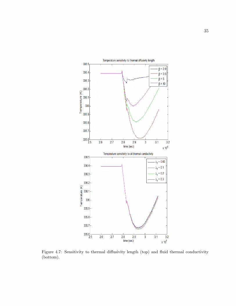
4.7 Sensitivity to thermal diffusivity length (top) and fluid thermal con-

ductivity (bottom). . . . . . . . . . . . . . . . . . . . . . . . . . . . . 35

4.8 Sensitivity to reservoir permeability (top) and fluid viscosity (bottom). 36

4.9 Sensitivity to gauge placement. . . . . . . . . . . . . . . . . . . . . . 37

4.10 Temperature estimation with b = 11m, over 0-350,000 data points

(left), actual data (right). . . . . . . . . . . . . . . . . . . . . . . . . 40

4.11 Temperature estimation with b = 8m, over 200,000-350,000 data points

(left), actual data (right). . . . . . . . . . . . . . . . . . . . . . . . . 40

4.12 Temperature estimation with b = 12m, over 300,000-400,000 data

points (left), actual data (right). . . . . . . . . . . . . . . . . . . . . . 41

4.13 Temperature estimation with b = 10m, over 100,000-200,000 data

points (left), actual data (right). . . . . . . . . . . . . . . . . . . . . . 41

vii

4.14 Two-dimensional marginal distribution of porosity and oil Joule-Thomson

coefficient from DAT.1. . . . . . . . . . . . . . . . . . . . . . . . . . . 43

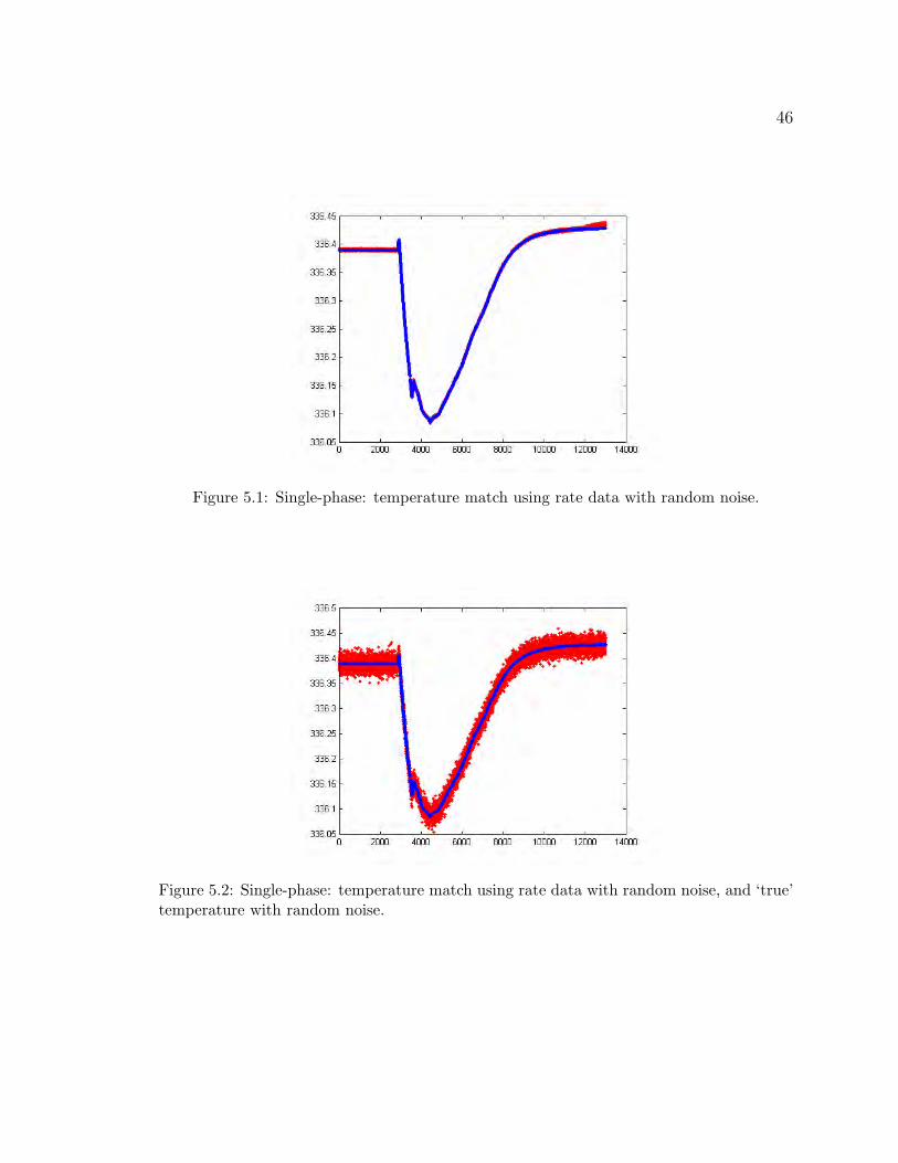
5.1 Single-phase: temperature match using rate data with random noise. 46

5.2 Single-phase: temperature match using rate data with random noise,

and ‘true’ temperature with random noise. . . . . . . . . . . . . . . . 46

5.3 Single-phase: temperature match with random noise added to the

‘true’ temperature. . . . . . . . . . . . . . . . . . . . . . . . . . . . . 47

5.4 Single-phase: temperature match using rate data with random noise,

with different transient region. . . . . . . . . . . . . . . . . . . . . . . 47

5.5 Two-phase: temperature match using rate data with random noise,

and ‘true’ temperature with random noise. . . . . . . . . . . . . . . . 48

5.6 Matching DAT.1 using OSATS (φ = 0.196, ε = −1.16 ∗ 10−7(K/Pa),

b = 9.2m). . . . . . . . . . . . . . . . . . . . . . . . . . . . . . . . . . 50


b = 6.12m). . . . . . . . . . . . . . . . . . . . . . . . . . . . . . . . . 50


b = 7.817m). . . . . . . . . . . . . . . . . . . . . . . . . . . . . . . . . 51


b = 5.2m). . . . . . . . . . . . . . . . . . . . . . . . . . . . . . . . . . 51


b = 3.0m). . . . . . . . . . . . . . . . . . . . . . . . . . . . . . . . . . 52


b = 5.16m). . . . . . . . . . . . . . . . . . . . . . . . . . . . . . . . . 52


b = 5.92m). . . . . . . . . . . . . . . . . . . . . . . . . . . . . . . . . 53

viii

5.13 Matching DAT.1 using fully numerical solution (φ = 0.286, ε = −1.53∗

10−8(K/Pa), b = 2.0m). . . . . . . . . . . . . . . . . . . . . . . . . . 54

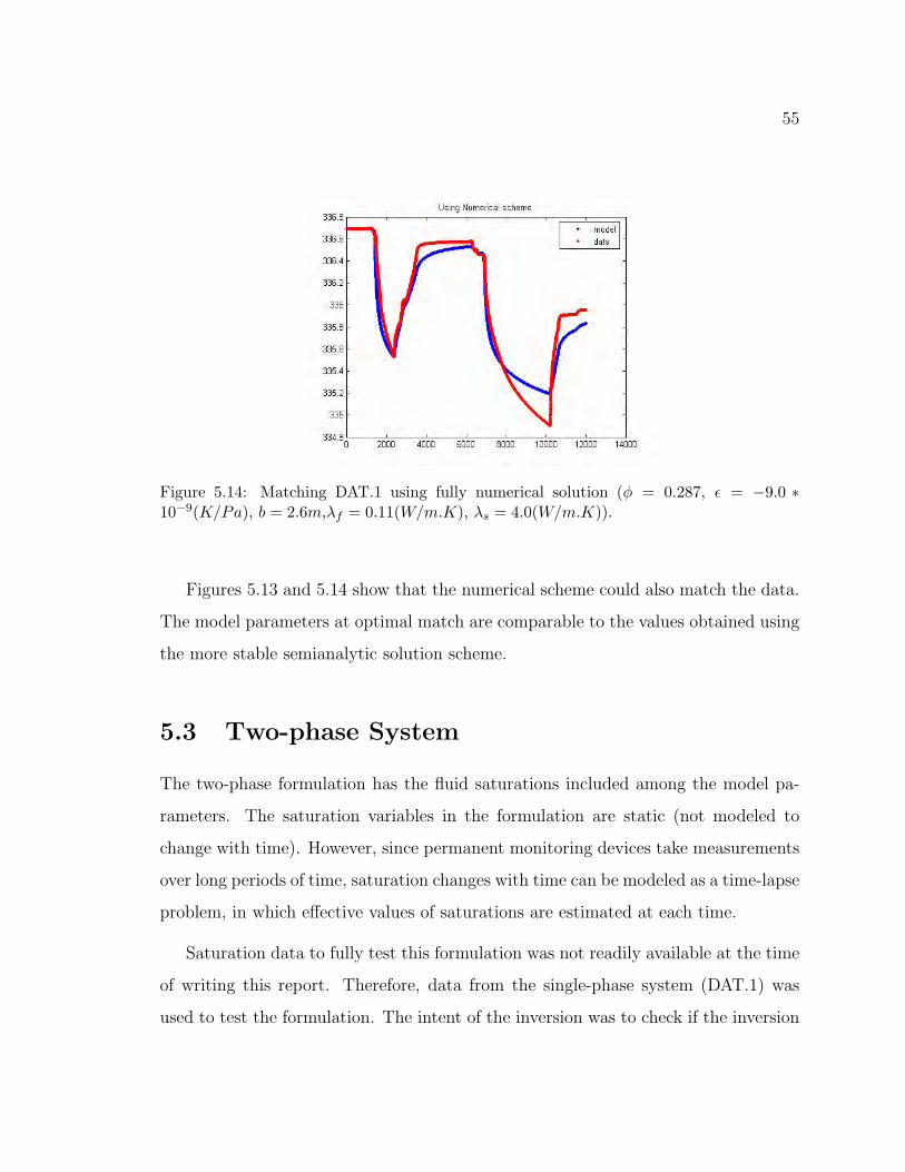
5.14 Matching DAT.1 using fully numerical solution (φ = 0.287, ε = −9.0 ∗

10−9(K/Pa), b = 2.6m,λf = 0.11(W/m.K), λs = 4.0(W/m.K)). . . . 55

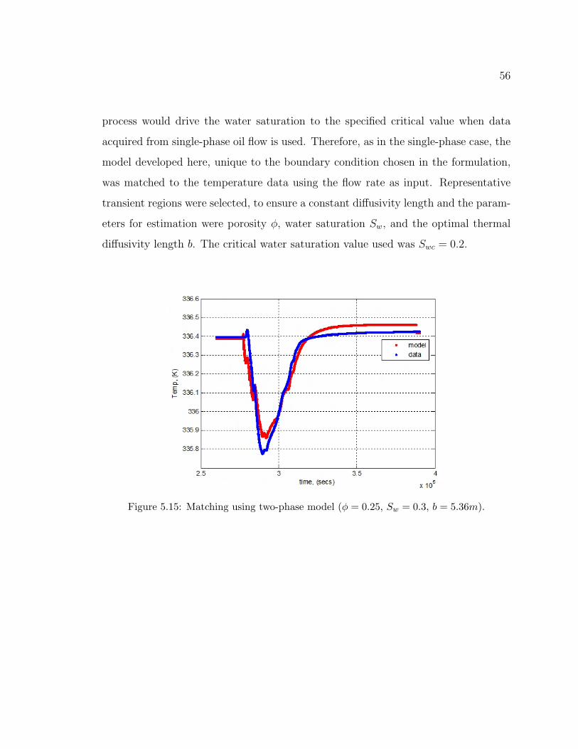
5.15 Matching using two-phase model (φ = 0.25, Sw = 0.3, b = 5.36m). . . 56

5.16 Three-dimensional spatial temperature distribution at a time instant

using DAT.1 data set. . . . . . . . . . . . . . . . . . . . . . . . . . . 58

5.17 Two-dimensional spatial temperature distribution at a time instant

using DAT.1 data set. . . . . . . . . . . . . . . . . . . . . . . . . . . 59

ix

Abstract

Permanent downhole gauges (PDGs) provide a continuous source of downhole pres-

sure, temperature and sometimes rate data. Until recently, the measured temperature

data have been largely ignored. However, a close observation of the temperature mea-

surements reveals that the temperature responds to changes in flow rate and pressure,

which implies that the temperature data may be a source of reservoir information.

In this work, the Alternating Conditional Expectations (ACE) technique was ap-

plied to temperature and flow rate signals from PDGs to establish the existence of

a functional relationship between them. Then, performing energy, mass and mo-

mentum balances, reservoir temperature transient models were developed for single-

and multiphase fluids, as functions of formation parameters, fluid properties, and

changes in rate and pressure. The pressure field in oil and gas bearing formations

are usually nonstationary. This gives rise to pressure-temperature effects appearing

as temperature changes in the porous medium when the pressure field is nonstation-

ary. The magnitudes of these effects depend on the properties of the formation, flow

geometry, time and other factors and result in a reservoir temperature distribution

that is changing in both space and time. Therefore, in this study, reservoir ther-

mometric effects were modeled as convective, conductive and transient phenomena

with consideration for time and space dependencies. This mechanistic model included

the Joule-Thomson effects due to fluid compressibility, and viscous dissipation in the

reservoir during fluid flow in accounting for the reservoir temperature dependence on

x

xi

changing pressure/flowrate fields.

Numerical solution schemes as well as the semianalytical scheme - Operator Split-

ting and Time Stepping (OSATS) were used to solve the models, and the solutions

closely reproduced the temperature profiles seen in real measured data. By matching

the models to different temperature transient histories obtained from PDGs, reservoir

parameters namely porosity and saturation and fluid Joule-Thomson coefficient could

be estimated. The significant contributions of this work include a method which:

• Utilizes temperature data measured by PDGs.

• Provides a way to estimate porosity and potentially saturation.

• May provide a less expensive substitute for downhole flow rate measurement.

Acknowledgements

I would like to thank my advisor Professor Roland Horne for his advice, guidance,

and encouragement through the course of this research.

Financial support from the Stanford Graduate Fellowship is greatly acknowledged.

The H.L. and Janet Bilhartz-ARCO Fellowship which was awarded to me was crucial

to the successful completion of this project.

Of course, I am grateful to my parents for their patience and love. My mother

- Lady Nelly Duru, whom I consider a lioness in character and in learning, and my

father - Sir Obinna Duru, a sheer genius. I would also like to thank my siblings for

their support.

I wish to thank the following: Uzoamaka (my best friend), my cousin Ijeoma

who refused to talk to me until I finished writing this report, Jerome (for being a

big brother), Antoine (for teaching me the French culture), Nilufer (for being a great

friend), Seun in UT Austin, and many others who in one way or the other have helped

shape my life.

Importantly, I can not thank ’Voke enough....although she was 7,814 miles away

from me, she offered to be my wake-up alarm every single morning and spurred me to

my responsibilities everyday. Her encouragements, support and concern were priceless

- she was there all the time, like my guardian angel.

xii

Chapter 1

Introduction

1.1 Background

Long term reservoir monitoring using permanent download monitoring devices has

been a continuous source of downhole data in the form of pressure, temperature and

sometimes flow rate. These tools provide access to data acquired continuously over

long periods of time which provide reservoir information at a much larger radius of

investigation than conventional wireline testing.

The behavior of pressure transients in reservoir and wellbore flow has been studied

extensively, and applied in conventional well test analysis for reservoir description,

parameter estimation for formation characterization and evaluation of well and field

performance. In recent times, with data convolution and deconvolution techniques as

well as data filtering and tuning, conventional pressure transient analytical methods

have also been applied to pressure data from permanent downhole gauges (PDGs),

increasing the usefulness of these data.

However, in conventional pressure transient analysis, the temperature distribu-

tions in the reservoir and wellbore have been assumed isothermal. The temperature

changes associated with fluid flow had been considered to be relatively small and

1

2

hence negligible for any consideration in the analysis of flow behavior of most flu-

ids. An analysis of temperature measurements, at a fine scale using continuous data

from PDGs, has shown that the temperature of the fluids responds to changes in flow

conditions in the reservoir. Generally, the flow is not isothermal when the scale of

observation and resolution of the temperature data is refined. This study attempts to

identify the underlying physical phenomena responsible for this temperature transient

behavior and its possible application to reservoir characterization and evaluation of

well performance.

1.2 Statement of the Problem

Many previous attempts at developing interpretation method for temperature profiles

in wellbore-reservoir systems have remained largely qualitative. Most of the analyses

have concentrated on wellbore thermal exchanges due to conduction and convection,

assuming that the produced fluid enters the wellbore at the geothermal temperature

Maubeuge et al. [12]. Others have attempted the study of thermometric fields in

reservoirs and porous systems, but have constrained the analyses to convective effects

only in steady-state formulations. A few have considered the effects of heating or

cooling of the produced fluid before it enters the wellbore due to factors like the

Joule-Thomson effect, adiabatic expansion and viscous dissipation.

The pressure field in oil and gas bearing formations are usually nonstationary [5].

This gives rise to pressure-temperature effects appearing as temperature changes in

the porous medium when the pressure field is nonstationary. The magnitudes of these

effects depend on the properties of the formation, flow geometry, time and other

factors, and result in a reservoir temperature distribution that is changing in both

space and time. Therefore, in this study, reservoir thermometric effects were modeled

as convective, conductive and transient phenomena with consideration for time and

3

space dependencies. This mechanistic model included the Joule-Thomson effects due

to fluid compressibility, and viscous dissipation in the reservoir during fluid flow in

accounting for the reservoir temperature dependence on changing pressure/flowrate

fields.

As a result of these investigations, it was found that in addition to establishing a

representative model for the temperature distribution in the reservoir, reservoir and

flow properties could be estimated in an inverse optimization problem.

Chapter 2

Literature Review

Several authors have studied the thermodynamics of flow through porous media and

wellbore systems, especially in the context of heat convection and conduction. One

of the earliest works in this regard was by Ramey [9] who developed a model for the

prediction of wellbore fluid temperature as a function of depth for injection wells.

Ramey expanded this model to give the rate of heat loss from the well to the for-

mation, assuming steady-state flow in the wellbore and unsteady radial conduction

in heat transfer to the earth. Horne and Shinohara [7] presented single-phase heat

transmission equations for both production and injection geothermal well systems by

modifying Ramey’s model as a way of calculating the heat losses between wellhead

and reservoir in order to evaluate reservoir temperature. Shiu and Beggs [20] pre-

sented another modification of Ramey’s model to predict the wellbore temperature

profile for a producing well, where the temperature of fluid entering the wellbore from

the reservoir is known. These wellbore models considered heat transfer as strictly con-

vection and conduction phenomena with fluid entering the formation at a constant

temperature from the reservoir.

Izgec et al.[8] presented a model that applied to coupled wellbore and reservoir sys-

tems and provided a transient wellbore temperature simulator coupled with a variable-

earth-temperature scheme for predicting wellbore temperature profiles in flowing and

4

5

shut-in wells. Again, their study looked at the mechanism of heat transfer in the

wellbore and the interaction with surrounding formation without consideration for

for possible changes in the reservoir fluid temperature before entry into the wellbore.

Sagar et al. [18], developed a steady-state two-phase model for the wellbore tem-

perature distribution accounting for Joule-Thomson effects due to heating/cooling

caused by pressure changes within the fluid during flow. They considered Joule-

Thomson effects as a possible heat source/sink during fluid flow and applied the

model to estimate heat losses in gas flow.

Valiullin et al. [22] presented a treatment of the temperature distribution in the

formation when the pressure field in the reservoir changes, and showed that indeed,

adiabatic and Joule-Thomson effects as well as effects due to heat of phase transition

(gas liberation from oil) may be present during fluid flow in a hydrocarbon satu-

rated porous medium. They designed experiments to estimate the thermodynamic

coefficients, namely the Joule-Thomson coefficient and adiabatic coefficients.

Ramazanov and Parshin [16] went on to develop an analytical model that described

the formation temperature distribution in a reservoir, while accounting for phase tran-

sitions. They solved a steady-state convective thermal flow model with constant flow

rate and extended it to cases with phase changes. In 2007, Ramazanov and Nagimov

[15] presented a simple analytical model to estimate the temperature distribution in

a saturated porous formation at variable bottomhole pressure. Their investigation

showed that for a single-phase fluid in a homogenous reservoir, temperature-pressure

effects such as Joule-Thomson can cause the temperature in the reservoir to very

significantly when reservoir pressure is changing in time. Ramazanov and Nagimov

solved the convective thermal transport model with variable pressure but constant

flow rate.

6

Attempts to solve the full energy balance equation for the temperature distribu-

tion in a reservoir was made by Dawkrajai [4] and Yoshioka [23]. Both presented

equations for reservoir and wellbore heat flow and developed prediction models for

the temperature and pressure. In an inversion step, they showed a means for the

identification of water and gas entry into a well. Both approaches made considera-

tions for Joule-Thomson and frictional heating effects but assumed a constant flow

rate, and steady-state conditions in arriving at the solution to their models.

Bear [1], Bejan [2] and Neild and Bejan [13] presented a comprehensive model

for heat transport in a porous media from mass, energy and momentum balance.

Thermal diffusion and convection and effects due to the fluid compressibility, vis-

cous dissipation (mechanical power required to extrude the fluid through the pore)

were incorporated into the model and the final form presented took the form of

a convection-diffusion model with source/sink terms. These studies discussed the

possibility of the optimization of the fluid space configuration for minimal thermal

resistance in a porous medium heat exchanger.

Chapter 3

Theory and Methodology

3.1 Introduction

In order to proceed with the study of the physics behind the observed temperature

response to changes in flow rate and pressure, as a reservoir temperature distribu-

tion problem, there is the need to establish the existence of a functional relationship

between the temperature, and pressure and flow rate. The technique chosen for this

investigation was the nonparametric regression tool, Alternating Conditional Expec-

tation (ACE) originally proposed by Breiman and Friedman [3]. ACE allows for the

estimation of optimal transformations that may lead to the maximal multiple corre-

lation between a response variable (temperature in this case) and a set of predictor

variables (pressure, rate and time). These transformations are useful in establish-

ing the existence of a functional relationship between the response variable and the

predictor variables.

7

8

3.2 Alternating Conditional Expectations (ACE)

ACE is a nonparametric iterative approach at estimating optimal transformations

of a data set to obtain maximal correlations between observed variables in the data

set. The power lies in its ability to perform this regression without making a priori

assumptions of functional forms of the relationships between the variables. The op-

timal transformations are based solely on the data set and unlike Neural Networks,

ACE can facilitate physically based function identification. ACE can also incorporate

multiple and mixed variables, both continuous (e.g. permeability, porosity, pressure)

and categorical (e.g. rock types).

3.2.1 Optimal Transformations[3]:

Given a real response (dependent) variable Y , and a p-dimensional vector X =

X1, ...Xp of predictor (independent) variables, define a set of arbitrary transforma-

tions θ(Y ), φ1(X1), ...φp(Xp). Suppose that a regression of the transformed response

variable on the sum of the transformed predictors result in the error:

e2(θ, φ1, ..., φp) = E

{[θ(Y )−

p∑i=1

θi(Xi)]2

}(3.2.1)

Then the transformations θ∗(Y ), φ∗1(X1), ..., φ∗p(Xp) are said to be optimal for the

regression if they satisfy that:

e∗2(θ∗, φ∗1, ..., φ∗p) = min

θ,φ1,...,φp

e2(θ, φ1, ..., φp) (3.2.2)

The correlation coefficient between the transformed response variable and sum of

the transformed predictor variables (under the constraints, E[θ2(Y )] = 1 and E[φ2s(X)])

is given by:

9

ρ(θ, φs) = E[θ(Y )φs(X)] (3.2.3)

where φs(X) =∑p

i=1 φi(Xi)

The optimal transformations θ∗(Y ), φ∗1(X1), ..., φ∗p(Xp) fulfill the maximal correla-

tion condition because, as shown in Breiman and Friedman [3], they satisfy that:

ρ∗(θ∗, φ∗s) = maxθ,φ1,...,φp

ρ(θ, φs) (3.2.4)

Breiman and Friedman [3] also showed that these optimal transformations for

correlation are also optimal for regression.

3.3 Mechanistic Modeling of Fluid Temperature

Transients

3.3.1 Distributed Reservoir Temperature Model

Theory of Thermometry in a Fluid-saturated Porous Media

The flow of energy-carrying fluids through a porous media has been studied for many

years. Bejan[2] and Bear[1] presented a comprehensive thermodynamic approach to

obtaining a representative model for temperature distribution in a porous media. The

model accounted for spatial distribution and well as transient effects in the formation.

Sharafutdinov[19], Filippov and Devyatkin[5] and Ramazanov and Nagimov[15] also

followed similar approaches in developing their models for temperature distribution

in a fluid saturated porous stratum.

In a flowing well, the pressure and flow rate measurements by permanent mon-

itoring gauges are not constant. For gauges placed close to the sandface flow area,

10

these changes reflect the dynamics of the flow in the reservoir. These flow dynamics

cause a temperature field to evolve in the reservoir, driven by thermodynamic effects

such as the Joule-Thomson heating (or cooling), adiabatic expansion, and heat of

phase transitions. Other effects namely the viscous dissipation, equal to the mechan-

ical power needed to extrude the viscous fluid through the pore, as well as frictional

heating between the fluid and rock matrix during the fluid flow are also factors that

contribute to the evolution of a nonuniform temperature field in the medium.

Joule-Thomson effect is the change in the temperature of a fluid due to expan-

sion or compression of the fluid in a flow process involving no heat transfer or work

(constant enthalpy). This change is due to a combination of the effects of fluid com-

pressibility and viscous dissipation. The Joule-Thomson effect due to the expansion

of oil in a reservoir or wellbore results in the heating of the fluid because of the value

of the Joule-Thomson coefficient of oil - it is negative for oil. The coefficient has a pos-

itive value for real gases and the consequent cooling effect is more prominent in gases.

Theoretically, the Joule-Thomson coefficient for ideal gases is zero implying that the

temperature of ideal gases would not change due to a pressure change if the system

is held at constant enthalpy. Combined with other factors, on expansion of the fluid

and subsequently flow of liquid oil and/or water out of the reservoir, the wellbore and

near wellbore areas in the reservoir become heated above the normal static reservoir

temperature. By convection, diffusion and further generation of heat enerygy due to

these effects, a nonuniform temperature is created, which spreads into the reservoir.

Conversely, during no-flow conditions (shut-ins), the regions already heated lose heat

to the surrounding formation through diffusion and result in a temperature decline

at a rate determined by the thermal diffusivity of the medium.

11

Reservoir Temperature Model in One-dimensional Cylindrical Coordinate

System

Single-phase Formulation

To derive the energy equation for a homogenous porous medium, the energy equations

for the solid and fluid parts are derived separately from the first law of thermody-

namics, and averaged over an elementary control volume to obtain the general form

of the model. The consideration is for a nonisothermal flow of a nonideal fluid in a

porous media. The change in kinetic and potential energies of the flow will be taken

as negligible.

For the solid part, assuming no internal heat generation per unit volume of the

solid material, the energy conservation equation associated with flow in an elastic

porous medium becomes:

ρscs∂T

∂t= ks

∂

∂rr∂T

∂r(3.3.1)

where (ρ, c, k)s are properties of the solid matrix.

The energy conservation equation at any point in space, occupied by the fluid is

given by:

ρfcpf

(∂T

∂t+ up

∂T

∂r

)= kf

∂

∂rr∂T

∂r+ βT

∂p

∂t+ βTv

∂p

∂r− v∂p

∂r+ vρg (3.3.2)

where (ρ, c, k)f are the fluid properties and T is the temperature for both the fluid

and solid. An assumption of local thermal equilibrium has been made between the

fluid and the porous matrix. Bejan[2] notes that this assumption is valid only for

small-pore media such as geothermal and oil reservoirs. Bejan[2] also showed that

Eqn. (3.3.1) and Eqn. (3.3.2) can be combined by volumetric averaging to give the

final form of the model as:

12

((1− φ)(ρscs) + φ(ρfcf ))∂T

∂t+ ρfcfv

∂T

∂r=

((1− φ)λs + φλf )

r

∂

∂rr∂T

∂r+ βTφ

∂p

∂t+ βTv

∂p

∂r− v∂p

∂r+ vρg (3.3.3)

On rearrangement and assuming negligible gravity effects, this becomes:

∂T

∂t+ u

∂T

∂r=α

r

∂

∂rr∂T

∂r+ ηφC

∂p

∂t+ εu

∂p

∂r(3.3.4)

The form of Eqn. (3.3.4) is the convection-diffusion type partial differential equa-

tion with source/sink terms. The second term on the right hand side of Eqn. (3.3.4)

is the compressibility term, while the last term is the viscous dissipation term.

The mass balance equation takes the form:

ρ∂ρf∂t

+1

r

∂(rvρf )

∂r= 0 (3.3.5)

The flow is assumed to obey Darcy’s law, and the equation for Darcy flow given

by

v =k

µ

∂p

∂r(3.3.6)

completes the formulation.

Where:

u = Cv

v = superficial velocity, ms

C = volumetric heat capacity ratio,cfcm

Cf = volumetric heat capacity of fluid, Jm3K

cm = (1− φ)(ρscs) + φ(ρfcf ) , volumetric heat capacity of fluid saturated rock, Jm3K

φ = porosity

ρ = density

13

η = βTCf

, adiabatic expansion coefficient, KPa

ε = βT−1Cf

, Joule-Thomson coefficient, KPa

β = 1ρ( ∂ρ∂T

)p , thermal expansion coefficient, 1K

α = λm

cm, thermal diffusivity, m2

s

λ = thermal conductivity, WmK

λm = φλf + (1− φ)λs, thermal conductivity of fluid saturated rock

Eqns (3.3.4), (3.3.5) and (3.3.6) form the governing equations for one-dimensional

thermal transport in a homogenous porous medium. The assumptions made in de-

riving the equations were:

• The medium is homogenous, such that the solid and fluid permeating the pores

are evenly distributed throughout the porous medium.

• The medium is isotropic such that permeability, k and thermal conductivity λ

do not depend on the direction of the experiment.

• At any point in the porous medium, the solid matrix is in thermal equilibrium

with the fluid in the pores.

• Darcy’s law applies.

Two-phase Formulation

The assumptions made for the two-phase formulation are similar to those made in the

single phase case, with the addition of negligible capillary effects. The thermal model

in a one-dimensional radial coordinate system for the two-phase system becomes:

14

((1− φ)(ρscs) + φ(ρwcfwsw + ρocfoso))∂T

∂t+ (ρwcfwswvw + ρocfosovo)

∂T

∂r=

((1− φ)λs + φ(λwsw + λoso))

r

∂

∂rr∂T

∂r+ (ρwcfwswηw + ρocfosoηo)φ

∂p

∂t

+ (ρwcfwswvwεw + ρocfosovoεo)∂p

∂r

(3.3.7)

On rearrangement and with negligible gravity and capillary effects, this becomes:

∂T

∂t+ u

∂T

∂r=α

r

∂

∂rr∂T

∂r+ η∗

∂p

∂t+ J∗

∂p

∂r(3.3.8)

The mass balance equation takes the form:

φ∂(ρwsw)

∂t+

1

r

∂(rvwρwsw)

∂r= 0 (3.3.9)

φ∂(ρoso)

∂t+

1

r

∂(rvoρoso)

∂r= 0 (3.3.10)

The Darcy flow equation becomes:

vw =kwµw.(∂pw∂r

) (3.3.11)

vo =koµo.(∂po∂r

) (3.3.12)

Where:

C = volumetric heat capacity ratio,(ρwcfwsw+ρocfoso)

cm


cm = (1− φ)(ρscs) + φ((ρwcfwsw) + (ρocfoso)) , volumetric heat capacity of fluid sat-

urated rock, Jm3K

η∗ =(ρwcfwswηw+ρocfosoηo

cm

)φ

15

J∗ =(ρwcfwswvwεw+ρocfosovoεo

cm

)η = βT

Cf, adiabatic expansion coefficient, K

Pa

ε = βT−1Cf


β = 1ρ( ∂ρ∂T


α = λm


s



subscripts:

w = water

o = oil

f = fluid

Eqns 3.3.8 through 3.3.12 are the equations defining the formulation for the tem-

perature distribution in a reservoir during two-phase flow. Eqn. 3.3.8 is a convection-

diffusion equation. Analytical solutions for convection-diffusion equations have been

the subject of research and numerical solutions have serious issues with stability due

in part to the nature of the model - a combination of a hyperbolic convective transport

and parabolic diffusion transport models. In this work, a semianalytical technique

used in ground water transport was used to solve this problem. The technique is

known as Operator Splitting and Time Stepping (OSATS), and was developed for the

solution of contaminant transport in ground water hydrology.[10][17]

3.3.2 Operator Splitting and Adaptive Time Stepping (OS-

ATS)

Kacur[10] and Remesikova[17] described methods for solving the convection-diffusion

type problem using the operator splitting approach. The operator splitting method

16

breaks the model into two different parts, the transport part and the diffusion part.

Then, at each time step, the nonlinear transport part and the nonlinear diffusion

part are solved separately. The semianalytical nature comes from the fact that the

solution is obtained in time sequences, with the solution at a time step depending on

the solution at all previous time steps. Holden et al.[6] showed the theoretical basis

for this technique.

Kacur[10] showed a precise way of solving the following type of problems:

∂F (u)

∂t+ v(x)

∂u

∂x− ∂

∂x(D(x, t))

∂u

∂x= f(x, u) (3.3.13)

with the boundary and initial conditions:

u(0, t) = co(t) (3.3.14)

u(L, t) = 0, for x ∈ (0, L), t > 0 (3.3.15)

u(x, 0) = uo(x) (3.3.16)

First, the transport part is solved, which presents a hyperbolic problem of the

form:

∂F (u)

∂t+ v(x)

∂u

∂x= 0, t ∈ (tj−1, tj) (3.3.17)

with boundary conditions of the form of Eqns. 3.3.14 and 3.3.15, and initial

condition of the form:

U(x, tj−1) = uj−1 (3.3.18)

17

The solution obtained is denoted as u1/2j := U(x, tj). Then the diffusion transport

part is solved, which has the form:

∂F (u)

∂t− ∂

∂x(D(x, t))

∂u

∂x= f(x, u), t ∈ (tj−1, tj) (3.3.19)

With the same boundary condition but with initial condition given by the solution

of the convective part -

U(x, tj−1) = u1/2j (3.3.20)

Finally, the solution at that time step is put as:

uj := U(x, tj) (3.3.21)

Which is the solution of Eqn. 3.3.19. This is continued until the solution at the

last time step is obtained, which becomes the final solution of the model.

3.3.3 Solution of the Thermal Convection-Diffusion Model

by OSATS

The OSATS approach was used to solve the thermal model Eqns. 3.3.4 and 3.3.8.

The methodology adopted was:

• Decouple the model into two parts: the convection transport part and the

diffusion part.

• At each time step, first solve the hyperbolic convection transport part, account-

ing for variable flow rate, as well as heat generation due to viscous dissipation,

frictional and Joule-Thomson effects.

• Then solve the diffusion part at the same time step, adaptively modifying the

time step to ensure stability if solution is numerical.

• Continue until the last time step.

18

Solution of the Single-phase Formulation by OSATS

The following assumptions were made in solving the single-phase reservoir thermal

model:

• Constant fluid Joule-Thomson, adiabatic expansion coefficient, and thermal

conductivity i.e. these parameters are assumed to be weak functions of temper-

ature

• Constant fluid viscosity and formation porosity

• Negligible gravity effects

A. Solution of the convective transport part:

The convection equation with its initial condition becomes:

∂T

∂t+ u

∂T

∂r= ηφC

∂p

∂t+ εu

∂p

∂r(3.3.22)

T (t = 0) = To(r) (3.3.23)

Using the method of characteristics, the solution yields:

dr

dt= u(r, t) = Cv(r, t) (3.3.24)

Such that for constant rate,

r2 = r21 +

qC

πh(t− t1) (3.3.25)

Another form of Eqn. 3.3.25 starts by solving for the pressure terms independently

from the material balance equation, and using the Darcy equation to replace velocity

in Eqn. 3.3.24. If the total compressibility of the porous medium is considered

negligible, then the pressure equation reduces to:

19

1

r

∂

∂rr∂p

∂r= 0 (3.3.26)

With boundary conditions:

p(r = re) = pe (3.3.27)

p(r = rw) = φ(t) (3.3.28)

where re = external radius and rw = wellbore radius.

This yields:

p(r, t) = pe +pe − φ(t)

ln(rerw

) . ln( r

re

)(3.3.29)

And:

∂p

∂r= [

pe − φ(t)

ln(rerw

) ].1

r(3.3.30)

Applying this to Eqn. 3.3.24 by replacing the velocity with the Darcy law equiv-

alent gives the form:

r2 = r21 − 2ψ(pet− s(t)) (3.3.31)

where:

ψ = kCµ lnR

,

R = ln rerw,

s(t) =t∫

0

Φ(τ)dτ

The parameter Φ(t) which is the sandface pressure (bottomhole pressure) in the well

bore is readily obtainable from solutions of classical pressure transient problems for

different reservoir models.

20

Alternatively, where the total compressibility of the system is not negligible, the

solution of the pressure equation comes in the form:

∆p =qµ

4πkhEi

(r2wπµct4kt

)(3.3.32)

Continuing the method of characteristics solution for the temperature yields,

dT

dt= ε

t∫0

dp

dtdt+ (η∗ − ε)

t∫0

∂p

∂τdτ (3.3.33)

with η∗ = ηφC.

This becomes:

T (r, t) = T0(r)− ε[p(r, 0)− p(r, t)]− η∗ − εlnR

t∫0

φ′(τ) ln

(r

re

)dτ (3.3.34)

Ramazanov and Nagimov [15] showed that by using the average time theorem,

the integral on the left hand side of Eqn. 3.3.35 can be closely approximated when

an optimal average time is used. Therefore, combining with Eqn. 3.3.31, and apply-

ing the average time theorem, the final approximate solution for wellbore sandface

temperature becomes:

T (rw, t) = T0(r1)− ε[p(r, 0)− φ(t)]− η∗ − εlnR

[φ(t)− φ(0)] ln

(√r21 − 2ψ(pez − s(z)

re

)(3.3.35)

where:

r1 =√r2w − 2ψ(pet− s(t) (3.3.36)

[0 ¡ z ¡ t]

z = average time.

21

An optimal choice for z must be used, and Ramazanov and Nagimov [15] suggested

t2< z < t.

B. Solution of the diffusion part:

The form of the diffusion problem is:

1

α

∂T

∂t=

1

r

∂T

∂r+∂2T

∂r2(3.3.37)

0 < r <∞

with initial and boundary conditions:

T (t = 0) = F (r) (3.3.38)

T (r = 0) = finite (3.3.39)

Ozisik [14] using the method of integral identity described by Masters [11], showed

that the solution to Eqn. 3.3.37 is of the form

T (r, t) =1

2αt

b∫r′

[r

′exp

(−r

2 + r′2

4αt

)F (r

′)Io

(rr

′

2αt

)]dr

′(3.3.40)

Where 0 < b < ∞ is equivalent to the thermal diffusivity length, and takes the

form b =√αt.

Therefore in operator splitting and time stepping approach, at each time step,

Eqn. 3.3.35 is evaluated for the solution of the convective part at that step. Then,

this solution forms the initial condition F (r) in the evaluation of the diffusion solution,

Eqn. 3.3.40. The final solution obtained from Eqn. 3.3.40 is taken as the temperature

of the system at that time step.

22

Solution of the Two-phase Formulation by OSATS

A. Solution of the convective transport part:

The convection equation with its initial condition is:

∂T

∂t+ C

∂T

∂r= η∗

∂p

∂t+ J∗

∂p

∂r(3.3.41)

T (t = 0) = To(r) (3.3.42)

The solution follows closely the approach used for single phase formulation.

By method of Characteristics,dr

dt= C (3.3.43)

For constant rate, let

qT = qo + qw (3.3.44)

qo =λoλTqT (3.3.45)

and

qw = qT − qo = qT

(1− λo

λT

)(3.3.46)

where:

λo = oil mobility(ko

µo

)λw = water mobility

(kw

µw

)λT = λo + λw

The solution to Eqn. 3.3.43 becomes

r2 = r21 +

qTπh

{ρwcfwsw(1− λo

λT) + ρocfoso

λoλT

}(t− t1) (3.3.47)

23

Again, we obtain another form of the solution Eqn. 3.3.47 by solving the pressure

equation, and using the Darcy equation to replace velocity in Eqn. 3.3.43. Assuming

total compressibility of the porous medium is negligible, then the pressure equation

reduces to:

1

r

∂

∂rr∂p

∂r= 0 (3.3.48)

with boundary conditions

p(r = re) = pe (3.3.49)

p(r = rw) = ϕ(t) (3.3.50)

where re = external radius and rw = wellbore radius.

Therefore,

p(r, t) = pe +pe − φ(t)

ln(rerw

) . ln( r

re

)(3.3.51)

and

∂p

∂r= [

pe − φ(t)

ln(rerw

) ].1

r(3.3.52)

Applying this to Eqn. 3.3.43 by replacing the velocity with the Darcy law equiv-

alent and solving gives

r2 = r21 − 2ψ(pet− s(t)) (3.3.53)

where

ψ ={ρwcfwswλw + ρocfosoλo}

cm lnR

R = lnrerw

24

s(t) =

t∫0

φ(τ)dτ

The parameter φ(t) which is the sandface pressure (bottomhole pressure) in the

well bore is readily obtainable from solutions of classical pressure transient problems

for multiphase flow, and for different reservoir models.

The temperature model therefore becomes,

dT

dt= ε∗

t∫0

dp

dtdt+ (η∗ − ε∗)

t∫0

∂p

∂τdτ (3.3.54)

where

ε∗ =ρwcfwswεwλw+ρocfosoεoλo

ρwcfwswλw+ρocfosoλo

This yields the solution

T (r, t) = T0(r)− ε∗[p(r, 0)− p(r, t)]− η∗ − ε∗

lnR

t∫0

ϕ′(τ) ln

(r

re

)dτ (3.3.55)

Using the average time theorem, the integral on the left hand side of Eqn. 3.3.55

can be closely approximated when an optimal average time is used. Therefore, the

final approximate solution for wellbore sand face temperature becomes:

T (rw, t) = T0(r1)−ε∗[p(r, 0)−φ(t)]− η∗ − ε∗

lnR[φ(t)− φ(0)] ln

(√r21 − 2ψ(pez − s(z)

re

)(3.3.56)

with

r1 =√r2w + 2ψ(pet− s(t))

0 < z < t, z = average time. An optimal choice for z must be used.

25

B. Solution of the diffusion part:

The form of the diffusion problem is

1

α

∂T

∂t=

1

r

∂T

∂r+∂2T

∂r2(3.3.57)

0 < r <∞

with initial and boundary conditions:

T (t = 0) = F (r) (3.3.58)

T (r = 0) = finite (3.3.59)

using the method of p− function and integral identity again, we get the solution

as

T (r, t) =1

2αt

b∫r′

[r

′exp

(−r

2 + r′2

4αt

)F (r

′)Io

(rr

′

2αt

)]dr

′(3.3.60)

Where 0 < b < is equivalent to the thermal diffusivity length, and takes the form

b =√αt.

The final form of the solution is obtained by following the operator splitting and time

stepping methodology used in the single-phase solution.

3.4 Numerical Solution

A fully numerical solution of the the model formulation would require a full dis-

cretization of the model. However, direct numerical solutions convection-diffusion

type PDEs with source/sink terms have been known to be very unstable. A way out

26

was to use Operator Splitting and Time Stepping (OSATS), in which case convec-

tive transport part was solved analytically (since it is easier to solve this way) and

numerical discretization methods were used the diffusion transport part.

The analytical solution of the convective transport problem has been shown in

preceding sections. In discretizing the diffusion part, the finite difference scheme was

adopted, and the coordinate system was taken to be cartesian. This gave:

1

α

∂T

∂t=

1

r

∂T

∂r+∂2T

∂r2(3.4.1)

Which became (in two-dimensional cartesian coordinate system) :

1

α

∂T

∂t=∂2T

∂x2+∂2T

∂y2(3.4.2)

1

αT n+1i,j − T n+1

i,j =1

∆x2Tni+1,j − T ni−1,j +

1

∆y2Tni,j+1 − T ni,j−1 (3.4.3)

subject to the same boundary and initial conditions.

Therefore, in the OSATS routine, at each time step, the convective problem was

solved analytically, while the diffusion problem was numerically approximated in the

central difference formulation shown in Eqn. 3.4.3 and solved in an explicit scheme.

3.5 Wellbore Temperature Transient Model

Permanent downhole monitoring tools are usually located some hundreds of feet (200

- 300 ft) above the perforation/production zone. The tool placement constraint is one

that is imposed by the design of the completions, and the optimal location for pressure

and temperature data management would be a position as close to the perforation as

possible, to give measurements that are comparable with their sandface values. This

calls for a coupling of the reservoir temperature model to a wellbore model to account

27

for heat loss that may occur between the fluid in the wellbore and the surrounding

formation when the fluid flows from the sandface to the gauge location.

The wellbore model used in this work was obtained from the work of Izgec et al.

[8]. The solution to the model is a modification of Ramey’s model [9] to account for

heat transfer at shut-in times when flow rate is zero and heat transfer in the wellbore

is only by conduction into the formation.

Izgec et al. [8] showed that the distribution of temperature in a wellbore can be

obtained, as a fucntion of depth, by

Tf (r, t) = Tei+1− eaLRt

LR

[1− e(z−L)LR

](gG sin θ + φ− (g sin θ)

cpJgc

)+e(z−L)LR (Tfbh − Tebh)

(3.5.1)

where

LR is called the relaxation parameter, defined by:

LR = 2πwcp

[rtoUtoke

ke+rtoUtoTD

]

with

TD = ln [e−0.2tD + (1.5− 0.3719e−tD)]√tD

tD = αtr2w

θ = wellbore inclination angel

φ = εdpdz

Tfbh = fluid temperature entering the sandface from formation (solution to the

reservoir temperature model)

Tei = geothermal temperature of formation at gauge location

28

Tebh = geothermal temperature of formation at bottomhole

3.6 Coupling the Reservoir Model to the Wellbore

Model

The issue of gauge placement, usually at some distance away from the perforation calls

for the coupling of the reservoir model to a wellbore model to account for heat loss

during flow between the perforation and the gauge location. In principle, the closer

the gauge to the perforation, the closer the overall model would be to the reservoir

model and the better the reservoir model can be used for further reservoir/formation

analysis.

The two models are coupled through the temperature of the fluid at the bottomhole.

The bottomhole temperature is estimated using the distributed reservoir model, and

used as an input into the wellbore model to estimate the fluid temperature at the

gauge location. The sensitivity of this overall model to the distance between the

gauge and the perforation will be revisited in a sensitivity analysis test to determine

the viability of using the model in reservoir studies, since the further away the gauge

is from the perforation, the less sensitive the solution will be to the reservoir model,

and more sensitive to the wellbore model.

Chapter 4

Qualitative Evaluation and

Sensitivity Analysis

4.1 Optimal Transformation for Estimation of Func-

tional Relationship

In order to show that a functional relationship may exist between temperature as a

response variable, and rate and pressure as the predictor variables, the nonparamet-

ric regression method known as Alternating Conditional Expectations (ACE) was

applied to a field data set. ACE yields optimal transformations of the variables,

and the correlations between these transformations have been shown to be optimal

for regression between the variables. These transformations are also useful in estab-

lishing the existence of a functional relationship between the response and predictor

variables. Using a field data set obtained from permanent downhole monitoring tool

in a well, the ACE method was applied to the pressure, rate and temperature data

to establish the existence or otherwise of a correlation and functional form for their

29

30

relationship. Figures 4.1 and 4.2 show the plots of rate, pressure and temperature

data, and the plot of the regression on the optimal transformations.

Figure 4.1: Flow rate data (left), pressure data (right) from DAT.1 data set.

Figure 4.2: Temperature data (left) from DAT.1 data set, optimal regression (right).

The optimal transformation functions showed a correlation coefficient of 0.99.

This means that temperature is well correlated with flow rate and pressure, that a

functional relationship may exist between temperature, and rate and pressure and

this functional form can be extracted from any representative data set.

31

4.2 Qualitative Evaluation of Model - Single-phase

Case

Having seen, from ACE analysis, that a functional form may exist between temper-

ature as a dependent variable, and rate and pressure as the independent predictor

variables, the mechanistic models developed for their relationship were tested quali-

tatively for a check of reproducibility of trends seen in the data used. Using arbitrary

but typical and physically meaningful values of the model parameters, the following

results were generated for qualitative evaluation of the model and the solution strat-

egy adopted here. The model were also checked for reproducibility of transient trends

seen in the measured data.

The input data sets used were flow rate information from two real fields, and here

called DAT.1 and DAT.2 data sets. These were obtained from permanent downhole

gauges (PDGs). The data sets consist of PDG measurements of flow rate, pressure and

temperature with time for different wells in different fields. Using the representative

flow rate data as input, and thermal model developed, the temperature profile was

simulated for each representative data input set.

Figures 4.3, 4.4, and 4.5 show that the model and the solution qualitatively cap-

tured the changes, effects and trends in the data, in acceptable details. The overall

shapes are reproduced by the formulation/solution using arbitrary model parameters.

This forms a motivation for performing sensitivity analysis on the model parameters,

for using the model in parameter estimation in an inverse problem and for subsequent

uncertainty analysis.

32

Figure 4.3: Qualitative comparison using DAT.1 (first representative transient).

Figure 4.4: Qualitative comparison using DAT.1 (second representative transient).

33

Figure 4.5: Qualitative comparison using DAT.2.

4.3 Sensitivity Analysis

Many variables/parameters are present in the model formulation and uncertainties

in their values present a challenge in further processing and utilization of the formu-

lation and solution methodology presented in this work, hence the need to test the

sensitivity of the formulation and solution to different values of these parameters.

The following parameters were tested for sensitivity of the solution to their values:

the porosity of the formation, Joule-Thomson coefficient of the fluids, reservoir thick-

ness, fluid viscosity, thermal conductivity of rock and fluid, permeability, thermal

diffusivity length, distance of permanent downhole gauge from the perforation and

the geothermal gradient.

34

Figure 4.6: Sensitivity to porosity (top) and fluid Joule-Thomson coefficient (bottom).

35

Figure 4.7: Sensitivity to thermal diffusivity length (top) and fluid thermal conductivity(bottom).

36

Figure 4.8: Sensitivity to reservoir permeability (top) and fluid viscosity (bottom).

37

Figure 4.9: Sensitivity to gauge placement.

It is clear from Figures 4.6 to 4.9 that the temperature formulation and solution is

sensitive to most of the model parameters. The parameters with the most prominent

sensitivity (> 50% in temperature estimation for <= 25% change in the value of the

parameters) were the fluid Joule-Thomson coefficient which smoothed the responses

to small intermittent rate changes, the porosity of the formation, the height of the

formation, the thermal diffusivity length, fluid viscosity and reservoir permeability.

However, since some of the parameters such as the formation thickness and geothermal

gradient can be estimated with acceptable certainty from other means such as well

logs, viscosity from laboratory measurements, as well as the gauge distance from

the perforation face, the parameter space for the inverse problem was reduced to

the space of formation porosity, fluid Joule-Thomson coefficient, thermal diffusivity

length and permeability. Porosity and permeability are highly correlated (as can be

seen also in the sensitivity plots). Therefore, in the inverse problem for parameter

38

estimation, permeability of the medium was specified, reducing the final parameter

space to formation porosity, formation thermal diffusivity length and fluid Joule-

Thomson coefficient. Sensitivity to the gauge distance presents a problem in using the

formulation presented in this work for possible reservoir parameter estimation. The

temperature of the fluid recorded at the gauge location is a combined effect of thermal

transient processes in the reservoir which delivers fluid of changing temperature (with

constant/changing rate) to the wellbore from the reservoir, and the heat loss to the

external formation during flow up the wellbore to the gauge location. This makes the

magnitude of heat loss in the wellbore very important, and calls for a careful use of

the formulation developed here if the gauge distance is very large. This is because,

at a very large distance away from the formation, the magnitude of the heat loss in

the wellbore will mask the effect of the reservoir thermal transients and hence lead to

poor reservoir parameter estimation. By repetitive trials, the optimal distance of the

gauge from the perforation to ensure obtaining representative reservoir parameters is

< 100m (300ft). This however is the average distance currently used in many field

applications.

Diffusivity length issues - single-phase

The challenge presented by the optimal selection of the diffusivity length parameter,

b, became apparent. Since this parameter depends on the thermal diffusivity and the

length of shut-in time (diffusion-dominated heat transfer period), different shut-in

regimes required different optimal diffusivity length because of differing shut-in time

durations.

As a test for this, the flow rate from DAT.1 data set (800 hrs, 466000 data points)

was used as input to the model to predict the temperature over the entire duration

of the measurement. Uniform thermal diffusivity length was assumed over several

39

transients and revealed a complete loss of the diffusion behavior later in time. Using

a uniform but different diffusivity length, b = 11m, over the data region 0 - 350,000

(data point counter on x-axis)(Figure 4.10), b = 8m over the data region 200,000 -

400,000,(Figure 4.11) and b = 12m over 300,000 - 400,000 (Figure 4.12). These plots

are shown only for qualitative reasons since model parameters were specified arbi-

trarily and were generated to see the behavior of the different shut-in regions with

different diffusivity length scale, as well as to reveal the effects later in time.

40

Figure 4.10: Temperature estimation with b = 11m, over 0-350,000 data points (left), actualdata (right).

Figure 4.11: Temperature estimation with b = 8m, over 200,000-350,000 data points (left),actual data (right).

41



The results show that while the model has the ability to predict the temperature

profile in the reservoir, the accuracy of that prediction depends on the diffusivity

42

length that characterizes the behavior of the profile at shut-in periods. No one dif-

fusivity length value will characterize the entire model over a long period of time

with recurring transients of different durations. Therefore, the optimal choice of this

length scale must be made and would not be one uniform value over several tran-

sient periods or over data taken for a relatively long time. Figure 4.13 shows that an

optimal selection should be found over each representative transient, separately and

independent of previous or subsequent shut-ins.

4.4 Sampling the Distribution of the Parameter

Space

The nature of the distribution of the parameter space is not known explicitly since the

model is nonlinear and the solution is semianalytic. Monte Carlo simulations was per-

formed to generate the one-dimensional and two-dimensional marginal distributions

of the parameter space. The distributions were then sampled for identification of the

optimal search space for parameter estimation, as well as to check for multimodalities

in the distribution of model parameters, using the method of volumetric probabilities

introduced by Tarantola [21]. The two-dimensional marginal distribution for the ra-

dial system, with porosity and oil Joule-Thomson coefficient as parameters is shown

in Figure 4.14.

43

Figure 4.14: Two-dimensional marginal distribution of porosity and oil Joule-Thomsoncoefficient from DAT.1.

Figure 4.14 shows that the distribution of the parameter space, in two-dimensional

marginal distribution sense is unimodal. The plots also show that the optimal pa-

rameter space for both porosity and oil Joule-Thomson coefficient as captured by the

model is within the feasible range and the values are physically realistic.

Chapter 5

Results and Discussion

The model solution, unique to the boundary condition chosen in the formulation, was

matched to the temperature data using the flow rate as input. In the case of field

data collected over long periods in time, because of thermal diffusivity length issues,

representative transient regions were selected, to ensure that a constant diffusivity

length could be used. In the optimization routine, the parameters that were perturbed

to establish the match were porosity φ, oil Joule-Thomson coefficient ε, fluid thermal

conductivity λf (in some instances as a check) and the optimal diffusivity length

b. The values of these parameters obtained at the optimal match were taken to be

estimates of the optimal values of the parameters.

5.1 Synthetic Data

As a check on the procedure, synthetic data were generated using the model devel-

oped in this work. The synthetic data were generated in three forms:

• normally distributed random noise (with mean 20% of the range of the flow

44

45

rate from DAT.1 data set) was added to the flow rate data, and this was used

as input to generate a temperature data set using the single-phase model

• again, normally distributed random noise was added to the temperature data

obtained above to create a second noisy temperature data set

• using a different transient region in DAT.1 data set, the step above was repeated

to generate a third temperature data set with appropriate noise added to it,

using the single-phase model

• the two-phase model was also used to generate a temperature data set

Each of the four temperature data sets above was used as ‘true’ measurement in

an inversion step to attempt to reestimate the model parameters used in generating

the data sets. This was done to test the robustness of the formulation and solution

strategy, and to examine the possibility of using them in an inverse model for param-

eter estimation.

46

Figure 5.1: Single-phase: temperature match using rate data with random noise.

Figure 5.2: Single-phase: temperature match using rate data with random noise, and ‘true’temperature with random noise.

47

Figure 5.3: Single-phase: temperature match with random noise added to the ‘true’ tem-perature.

Figure 5.4: Single-phase: temperature match using rate data with random noise, withdifferent transient region.

48

Figure 5.5: Two-phase: temperature match using rate data with random noise, and ‘true’temperature with random noise.

For Figure 5.1, the data were generated using φ = 0.3, ε = 4.5 ∗ 10−8(K/pa)

and b = 7.0m. The optimal parameter values after the match were φ = 0.227, ε =

3.5 ∗ 10−8(K/pa) and b = 7.3m.

In Figure 5.2, the data were generated using φ = 0.3, ε = 4.5 ∗ 10−8(K/pa) and

b = 7.0m and the match occurred at φ = 0.231, ε = 3.27 ∗ 10−8(K/pa) and b = 7.2m.

In Figure 5.4, the data were generated with φ = 0.3, ε = 4.5 ∗ 10−8(K/pa) and

b = 8.0m and the match occurred at φ = 0.259, ε = 1.51 ∗ 10−8(K/pa) and b = 8.32m

Finally, in the two-phase case shown in Figure 5.5, the data were generated with

φ = 0.3, Sw = 0.45 and b = 2.7m and the match occurred at φ = 0.145, Sw = 0.493

and b = 3.0m.

The plots show good matches between the ‘true’ data and simulated results for

the tests on both models (single- and two-phase models). Also, the values of the

49

model parameters obtained after the matching were close to the original values of

the parameters. This shows that the formulation with the solution method used was

able to closely reestimate the parameters used in generating a synthetic data set and

so lends support to the attempt to use the model formulation in an inverse step for

reservoir parameter estimation by matching the model to real field temperature data.

5.2 Field Data

5.2.1 Single-phase System

Two different sets of field data were used to test the model, as well as obtain model

parameters at optimal match of the model to the data. The data sets have been named

DAT.1 and DAT.2. DAT.1 set is an 800-hr long measurement, each measurement

taken every 6 secs. DAT.2 is 24-hr long with each measurement taken every second.

Again, representative transient regions were selected, to ensure a constant diffusivity

length and the parameters for used in the inverse problem were porosity φ , oil Joule-

Thomson coefficient ε, fluid thermal conductivity λf (in some instances as a check)

and the thermal diffusivity length b.

The following plots were obtained using the semianalytical solution technique (Op-

erator Splitting and Adaptive Time Stepping [OSATS]) discussed in Chapter 3.0, and

the values of the model parameters at optimal match are shown in the caption of each

figure.

50

Figure 5.6: Matching DAT.1 using OSATS (φ = 0.196, ε = −1.16∗10−7(K/Pa), b = 9.2m).

Figure 5.7: Matching DAT.1 using OSATS (φ = 0.21, ε = −9.0 ∗ 10−9(K/Pa), b = 6.12m).

51

Figure 5.8: Matching DAT.1 using OSATS (φ = 0.235, ε = −4.48 ∗ 10−8(K/Pa), b =7.817m).

Figure 5.9: Matching DAT.1 using OSATS (φ = 0.2, ε = −7.7 ∗ 10−8(K/Pa), b = 5.2m).

52



53

Figure 5.12: Matching DAT.2 using OSATS (φ = 0.182, ε = −5.95 ∗ 10−8(K/Pa), b =5.92m).

Figures 5.6 to 5.11 show good matches between the single-phase model and DAT.1

data set. Figure 5.12 also show the match using the single-phase model on DAT.2

data set. Both direct search (Genetic algorithms) and gradient based (Levenberg

Marquardt) optimization techniques were used in the inverse problem to run each

case, and the optimal parameters at the matches were always approximately equal

for each optimization algorithm used. These values of the model parameters (also

reservoir and fluid properties) obtained at optimal match are physically meaningful,

and the porosity values are well within the range of porosity values for carbonate

reservoirs (for DAT.1 data set), the Joule-Thomson coefficient values also satisfy the

range of values of the coefficient that have been obtained for different types of crude

oil. The thermal diffusivity length correlation to the duration of shut-in for each

transient is also very obvious. The longer the shut-in (when input flow rate is zero),

the longer the optimal thermal diffusivity length estimated from the inverse problem.

54

A fully numerical solution of the the model formulation was also attempted

for comparison with results from the semianalytical solution. It must be noted

that numerical solution to convection-diffusion problems, especially where there are

source/sink terms, are known to be very unstable. A way out was to use Opera-

tor Splitting and Time Stepping (OSATS), in which case numerical discretization

methods were used to solve each of the decoupled convection and diffusion transport

parts.

Figure 5.13: Matching DAT.1 using fully numerical solution (φ = 0.286, ε = −1.53 ∗10−8(K/Pa), b = 2.0m).

55

Figure 5.14: Matching DAT.1 using fully numerical solution (φ = 0.287, ε = −9.0 ∗10−9(K/Pa), b = 2.6m,λf = 0.11(W/m.K), λs = 4.0(W/m.K)).

Figures 5.13 and 5.14 show that the numerical scheme could also match the data.

The model parameters at optimal match are comparable to the values obtained using

the more stable semianalytic solution scheme.

5.3 Two-phase System

The two-phase formulation has the fluid saturations included among the model pa-

rameters. The saturation variables in the formulation are static (not modeled to

change with time). However, since permanent monitoring devices take measurements

over long periods of time, saturation changes with time can be modeled as a time-lapse

problem, in which effective values of saturations are estimated at each time.

Saturation data to fully test this formulation was not readily available at the time

of writing this report. Therefore, data from the single-phase system (DAT.1) was

used to test the formulation. The intent of the inversion was to check if the inversion

56

process would drive the water saturation to the specified critical value when data

acquired from single-phase oil flow is used. Therefore, as in the single-phase case, the

model developed here, unique to the boundary condition chosen in the formulation,

was matched to the temperature data using the flow rate as input. Representative

transient regions were selected, to ensure a constant diffusivity length and the param-

eters for estimation were porosity φ, water saturation Sw, and the optimal thermal

diffusivity length b. The critical water saturation value used was Swc = 0.2.

Figure 5.15: Matching using two-phase model (φ = 0.25, Sw = 0.3, b = 5.36m).

57

Figure 5.15 shows the plots of the match of the two-phase model to data single-

phase system. Since the data set used was that from a single-phase oil flow, the

inversion optimization step was expected to drive the water saturation to its critical

value at optimal match. The initial value of water saturation was set at 0.6. Then a

gradient-based search was used to obtain the match of the model to the data. The

estimated value of water saturation at optimal match (according to tolerance set on

the optimization routine) was Sw = 0.28. The algorithm drove the water saturation

towards the critical water saturation specified, at each iteration. Using direct search

(Genetic algorithm), similar results were also obtained.

5.4 Potential Applications

The models developed in this study have been shown to have the potential to help

characterize a reservoir using only rate and temperature data from any permanent

downhole monitoring source. Until recently, temperature data measured have been

largely ignored. Specifically, this study provides a method for the estimation of poros-

ity in homogenous fields, as well as potential for estimation of saturation distribution

in a reservoir using temperature data only. Being rate-dependent, the temperature

data could also offer a way to estimate sandface flowrate by inverting the temperature

model to estimate flowrate.

Spatial distribution of porosity and saturation fields

(heterogeneous field preliminary study)

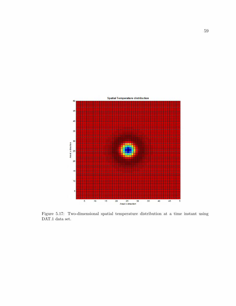
The formulations and their solutions allow for local point-to-point estimation of tem-

perature in a discretized spatial grid. Each local estimation is dependent on the local

values of the model parameters, hence allowing for the estimation of local (grid) val-

ues of model parameters, each depending on the value of the temperature at the grid.

58

This forms the basis for the estimation of heterogeneous parameter fields. Results

can serve as secondary conditioning data for porosity and saturation fields in reservoir

modeling. Examples of such estimations are shown in Figures 5.16 and 5.17.

Figure 5.16: Three-dimensional spatial temperature distribution at a time instant usingDAT.1 data set.

Data from interference well testing or horizontal wells could be used in check-

ing/validating these characterization of temperature fields in space.

59

Figure 5.17: Two-dimensional spatial temperature distribution at a time instant usingDAT.1 data set.

Chapter 6

Scope for Further Study

6.1 Updating the Boundary Conditions

Only one boundary condition has been specified in the solution obtained in this

problem (bounded for convective, infinite radial for diffusion). Different reservoir

configurations will require different boundary condition (e.g. where the reservoir is

bounded by an aquifer), and will require the specification of the appropriate boundary

conditions in the solution.

6.2 Updating the Model to Treat Three-phase Sys-

tems (Gas-Oil-Water)

The formulations presented in this study considered single-phase oil, and two-phase

oil-water systems. In a single-phase gas system, some conditions and assumptions

made must be relaxed to accommodate specific physical conditions that come with

gas systems. For example, gas densities are not constant and are specifically affected

60

61

by changes in temperature. Similarly, gas thermal conductivity is a strong function

of temperature as well as gas viscosities. Most of these conditions were relaxed in

building the single-phase oil model. Similar considerations must also be made in

developing the three-phase gas-oil-water model.

6.3 Reservoir Models with Fluid Injection or Phase

Transition

The formulation in this study assumed no fluid injection and considered temperature

changes due strictly to fluid expansion and viscous dissipation. However, the idea

behind the model can be extended to also account for cases where there is fluid

injection into the reservoir. Similarly, phase transitions (e.g. liberation of free gas in

the reservoir) can also be considered for a more complete picture of thermal effects

in the reservoir.

6.4 Cointerpretation of Pressure, Rate and Tem-

perature

This model presents an additional source of information in transient analysis - tem-

perature. Using ACE, it was shown that a functional relation exists between temper-

ature, rate and pressure. This presents the possibility of cointerpreting rate, pressure

and temperature.

62

6.5 Heterogenous Fields

As shown earlier, if the appropriate data is available (e.g. temperature distribution

in space from a horizontal well, or temperature measured at different wells producing

from the same reservoir - interference testing), the spatial distribution of the model

parameters could be estimated and used to characterize the heterogenous fields of

porosity and saturation.

Nomenclature

b = thermal diffusivity length, m C = volumetric heat capacity ratio,(ρwcfwsw+ρocfoso)

cm


cm = (1− φ)(ρscs) + φ((ρwcfwsw) + (ρocfoso)) , volumetric heat capacity of fluid sat-

urated rock, Jm3K

p = pressure, Pa q = flowrate m3

s

r = radius

T = temperature, K

Tfbh = fluid temperature entering the sandface from formation (solution to the reser-

voir temperature model)

Tei = geothermal temperature of formation at gauge location

Tebh = geothermal temperature of formation at bottomhole

tD = dimensionless time αtr2w

Uto = overall heat transfer coefficient, J(secKm2)

u = Cv

v = superficial velocity, ms

Greek

φ = porosity

ρ = density

η = βTCf

, adiabatic expansion coefficient, KPa

ε = βT−1Cf


β = 1ρ( ∂ρ∂T


α = λm


s



63

64

θ∗ = optimal transformation of the dependent variable

φ∗ = optimal transformation of the independent variables

θ = wellbore inclination angel

φ = εdpdz

subscripts:

w = water

o = oil

f = fluid

References

[1] J. Bear, The Dynamics of Fluids in Porous Media, Dover Publications, Inc, 1972.

[2] A. Bejan, Convective heat transfer, Wiley, 2004.

[3] L. Breiman and J.H. Friedman, Estimating optimal transformation for multiple

regression and correlation, Journal of American Statistical Association 80 (1985),

no. 391, 580–598.

[4] P. Dawkrajai, A.R. Analis, K. Yoshioka, D. Zhu, A.D Hill, and L.W Lake, A

comprehensive statistically-based method to interpret real-time flowing measure-

ments, DOE Report (2004).

[5] A.I. Filippov and E.M. Devyatkin, Barothermal effect in a gas-bearing stratum,

High Temperature 39 (2001), no. 2, 255–263.

[6] H. Holden, K.H. Larlsen, and K.A. Lie, Operator splitting methods for degen-

erate convection-diffusion equations, II: Numerical examples with emphasis on

reservoir simulation and sedimentation, Comput. Geosci. 4 (2000), 287–323.

[7] R.N. Horne and K. Shinohara, Wellbore heat loss in production and injection

wells, J. Pet. Tech (1979), 116–118.

[8] B. Izgec, C.S. Kabir, D. Zhu, and A.R. Hasan, Transient fluid and heat flow

modeling in coupled wellbore/reservoir systems, SPE 102070 presented at the

SPE Annual Technical conference, San Antonio, Texas (Sept. 2006).

65

66

[9] H.J Ramey Jr., Wellbore heat transmission, JPT 435 (1962).

[10] J. Kacur and P. Frolkovic, Semi-analytical solutions for contaminant transport

with nonlinear soption in one dimension, University of Heidelberg, SFB 359 24

(2002), 1–20.

[11] J.I. Masters, Some applications of the p-function, Journal of Chem. Physics 23

(1955), 1865–1874.

[12] F. Maubeuge, M. Didek, M.B. Beardsell, E. Arquis, O. Bertrand, and J.P. Cal-

tagirone, Mother:a model for interpreting thermometrics, SPE 28588 presented

at the SPE Annual Technical Conference and Exhibition (Sept. 1994).

[13] D.A. Neild and A. Bejan, Convection in porous media, Springer, 1999.

[14] M.N. Ozisik, Heat conduction, Wiley-Intersciences, 1993.

[15] A. Sh. Ramazanov and V.M. Nagimov, Analytical model for the calculation of

temperature distribution in the oil reservoir during unsteady fluid inflow, Oil and

Gas Business Journal (2007).

[16] A. Sh. Ramazanov and A.V. Parshin, Temperature distribution in oil and water

saturated reservoir with account of oil degassing, Oil and Gas Business Journal

(2006).

[17] M. Remesikova, Solution of convection-diffusion problems with nonequilibrium

adsorption, Journal of Comp. and Applied Maths 169 (2004), 101–116.

[18] R.K. Sagar, D.R. Dotty, and Z. Schmidt, Predicting temperature profiles in a

flowing well, SPE 19702 presented at SPE Annual Technical Conference and

Exhibition, San Antonio, TX (1989).

67

[19] R.F. Sharafutdinov, Multi-front phase transitions during nonisothermal filtration

of live paraffin-base crude, Journal of Applied Mechanics and Techincal Papers

42 (2001), no. 2, 284–289.

[20] K.C. Shiu and H.D. Beggs, Predicting temperatures in flowing oil wells, J. Energy

Resources Tech (1989), 1–11.

[21] A. Tarantola, The Inverse Problem Theory and Model Parameter Estimation,

SIAM, 2005.

[22] R.A. Valiullin, R.F. Sharafutdinov, and A.Sh. Ramazanov, A research into ther-

mal fields in fluid-saturated porous media, Elsevier 148 (2004), 72–77.

[23] K. Yoshioka, Detection of water or gas entry into horizontal wells by using per-

manent downhole monitoring systems, Ph.D. thesis, Texas A and M University,

Department of Petroleum Engineering, 2007.

Appendix

Matlab program files

Main calling file

%%%%%%%%%%%%%%%%%%%%%%%%%%%%%%%%%%%%%%%%%%%%%%%%%%%%%%%%%%%%%

%%% Main Calling file. Main file for the optimization routine%%

%%%%%%%%%%%%%%%%%%%%%%%%%%%%%%%%%%%%%%%%%%%%%%%%%%%%%%%%%%%%%%%

clear all

clc

% x is the vector of parameters to be estinated. It comes as the vector

% [phi e bb lambdaf lambdas] where phi = porosity, e = JT coeff, lambda = thermal

% conductivity, bb = thermal diffusivity length. The vector x can be any

% length depending on number of parameters specified for estimation

display ’ Using Tsimulator......’

%%%Initial Guess

phid0 = log(0.300/0.2); ed0 = log((9.0*10^-8)/(8.0*10^-8)); bd0 = log(150/100);

lamdf0 = log(0.15/0.12); lamds0 = log(3/2); %re = log(100/100); h = log(30/30); nn = log(90/90);

x0 = [phid0 ed0 bd0 lamdf0 lamds0];% re h nn];

lb = [-1.08 -5.0 -2.350 -2.49 -1.386];% -3.3 -1.79 -1.5];

ub = [.9163 4.22 1.9163 1.200 0.9100 ];%3.30 1.500 2.05];

TypX = [phid0 ed0 bd0 lamdf0 lamds0];% re h nn];

%%%Optimization routine

nvars = 6;

[x, fval] = ga(@ParEstm,nvars,[],[],[],[],lb,ub); % Using Genetic algorithm, a direct search method

%%%Other algorithms to use

68

69

% options = saoptimset(’TolFun’,1.00e-6);

% [x, fval] = simulannealbnd(@ParEstm,x0,lb,ub,options); % Using simulated

% annealing

% options = optimset(’LevenbergMarquardt’,’on’,’LargeScale’, ’off’,’MaxFunEvals’,2000,’TypicalX’,TypX,’Jacobian’,’off’,’TolFun’,1e-15,’TolX’,1e-15,’TolCon’,1e-15);

% [x,fval,exitflag,output,lambda,grad,hessian] = fmincon(@ParEstm,x0,[],[],[],[],lb,ub,[],options); % Using LevenbergMarquardt

% options = optimset(’LevenbergMarquardt’,’off’,’LargeScale’, ’on’,’MaxFunEvals’,2000,’Jacobian’,’off’,’TypicalX’,TypX,’TolFun’,1e-10,’TolX’,1e-10);

% %

% [x,resnorm,residual,exitflag,output,lambda,jacobian] = lsqnonlin(@ParEstm,x0,lb,ub,options);

% % %%%%%%%%%%%%%%%%%%%%%%%%%%%%%%%%%%%%%%%%%%%%%%%%%%%%%%%%%

%%%%%%%%%%%%%%%%%%%%%%%%%%%%%%%%%%%%%%%%%%%%%%%%%%%%%%%%%%%%%%%%%%

%%ParEstimation program

function [F] = ParEstm(x)

x = real(x);

% load data

load B5.dat

time = B5(1:length(B5),1)*3600; %Time count (s),

press = B5(1:length(B5),2)*6894; %Pressure data, pa

temp = B5(1:length(B5),3) + 273.15; %Temperature data, K

rate = B5(1:length(B5),4)*0.00000184; %rate (m^3/sec)

P=press;

q=rate;

t=time;

Te=345.1; % Initial reservoir temperature, K

[ObjFunc] = ObjFun(P,q,t,temp,x,Te);

F = sqrt(sum(ObjFunc.^2));

[fid] = fopen(’ResidualTrack.txt’,’at+’);

fprintf(fid, ’%10.6f\n’,ObjFunc);

fclose(fid);

[fid] = fopen(’ParTrack.txt’,’at+’);

70

phi = 0.2*exp( x(1)); %porosity

e = (8.0*10^-8)* exp(x(2)); % % Joule thomson coefficient, K/Pa

bb = 100. * exp(x(4));

lamdf = 0.12*exp(x(5));

lamds = 2.0*exp(x(6));

% re = 100.*exp(x(7));

% h = 30.*exp(x(8));

% nn = 90.*exp(x(9));

fprintf(fid, ’%10.6f %10.12f %10.7f %10.6f %10.7f\n’,phi, e, bb, lamdf, lamds);% re, h, nn);

fclose(fid);

Resnorm = sqrt(sum(ObjFunc.^2));

[fid] = fopen(’ResNormTrack.txt’,’at+’);

fprintf(fid, ’%10.6f\n’,Resnorm);

fclose(fid);

%%%%%%%%%%%%%%%%%%%%%%%%%%%%%%%%%%%%%%%%%%%%%%%%%%%%%%%%%%%%%%%%%%%%%%%%%%%%%%%%%%

function [ObjFunc] = ObjFun(P,q,t,temp,x,Te)

%cfct= 2.*exp(x(3));

[Tmodel, init, fnl] = Tsim(P,q,t,x);

Tdata = temp(init:fnl);

Tcalc = (Te + Tmodel’);

ObjFunc = Tdata - Tcalc;

% fopen(figure(1));

% plot((Te+Tmodel*x(3)),’*r’);

% hold on;

%%%%%%%%%%%%%%%%%%%%%%%%%%%%%%%%%%%%%%%%%%%%%%%%%%%%%%%%%%%%%%%%%%%%%%%%%%%%%%%%%%%%%

function [Tmodel, init, fnl] = Tsim(P,q,t,x)

%% Parameters for Estimation

% phi = x(1); %porosity

% e = x(2); % % Joule thomson coefficient, K/Pa

71

% %lambdaf = x(3);

% cfct= x(3); % correction for wellbore heat loss

% bb = x(4);

phi = 0.2*exp( x(1)); %porosity

e = (8.0*10^-8)* exp(x(2)); % % Joule thomson coefficient, K/Pa

cfct= 2.0 * exp(x(3)); % correction for wellbore heat loss

bb = 100. * exp(x(4)); % Thermal diffusivity length, m

lambdaf = 0.12*exp(x(5)); %oil thermal conductivity, W/m.K

lambdas = 2.0*exp(x(6)); %formation rock thermal conductivity, W/m.K

%% fluid property

cf=1880; %oil spec heat, J/Kg.K

n=1.*10^-9; %adiabatic expansion coeff, K/Pa

beta= 0.001206; %thermal expansion coeff, 1/K

mu= 0.005; %current is from STARS at 157 F, 0.005; %viscosity, Pa.s

rhof=800; %oil density, Kg/m^3

%% Reservoir skeleton property/geometry

k = .7*10^-12; %permeability (2D), m^2

cs = 1000; %specific heat of solid, J/Kg.K

rhos=2300; %rock density, Kg/m^3

re=1000; % reservoir external radius, m

h=40; % reservoir height, m

D=3500; % well depth, m

zz=3400; % position of PDG above production zone, m

gG=0.0364; % geothermal gradient, K/m

g=9.81; % acceleration due to gravity, m/sec^2

cT=3.0; %

alphas=1.03*10^-6; % earth thermal diffusivity, m^2/sec

%% Wellbore property

rti=0.03; % tube inner radius, m

rto=0.04445; % tube outer radius, m

rci=0.08433; % casing inner radius, m

rco=0.0889; %casing outer radius, m

rwb=0.1; % wellbore radius, m

72

%% combined property

ct= 1.16*10^-8; % formally *10^-8 % total compressibility, 1/Pa

cres=((1-phi)*(rhos*cs))+(phi*rhof*cf); % saturated reservoir volumetric heat capacity, J/K.m^3

%lambdar=((1-phi)*(lambdas*cs))+(phi*lambdaf*cf); %

lambdar=((1-phi)*(lambdas))+(phi*lambdaf);% saturated reservoir thermal conductivity, W/m.K

c=(rhof*cf)/cres;% vol heat capacity fraction, dim’less

Ti=335.377; % Initial reservoir temperature, K

Pe = 3.2*10^7; % Initial reservoir pressure, pa

alpham=lambdar/cres; % thermal diffusivity of fluid saturated rock, m^2/sec

%%

R=re/rwb;

nu_x=n*phi*c;

big_phi = k*c/(mu*log(R));

T1 = 0.0;

q = q(7750:9000);

t = t(7750:9000);

init = 7750;

fnl = 9000;

diff = (fnl - init)+1;

% z = zeros(1,diff);

% phi_t = zeros(1,diff);

% M = zeros(1,diff);

% TT = zeros(1,diff);

% Ttt2 = zeros(1,diff);

% Ttt12 = zeros(1,diff);

% TT1 = zeros(1,diff);

% T = zeros(1,diff);

z(1) = (4/5)*t(1);

for i=2:diff

M(i) = (((q(i)-q(i-1))*mu/(4*pi*k*h))*(expint(rwb^2*phi*mu*ct/(4*k*(t(i)-t(i-1))))));

phi_t(i)=Pe + M(i);

tD(i) = k*t(i)/(phi*mu*ct*rwb^2);

tD = tD(i);

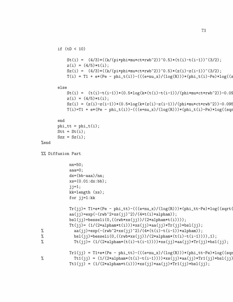
73

if (tD < 10)

St(i) = (4/3)*((k/(pi*phi*mu*ct*rwb^2))^0.5)*(t(i)-t(i-1))^(3/2);

z(i) = (4/5)*t(i);

Sz(i) = (4/3)*((k/(pi*phi*mu*ct*rwb^2))^0.5)*(z(i)-z(i-1))^(3/2);

T(i) = T1 + e*(Pe - phi_t(i))-(((e+nu_x)/(log(R)))*(phi_t(i)-Pe)*log((sqrt(rwb^2 + 2*big_phi*St(i) - 2*big_phi*Sz(i)))/re));

else

St(i) = (t(i)-t(i-1))*(0.5*log(k*(t(i)-t(i-1))/(phi*mu*ct*rwb^2))-0.095465);

z(i) = (4/5)*t(i);

Sz(i) = (z(i)-z(i-1))*(0.5*log(k*(z(i)-z(i-1))/(phi*mu*ct*rwb^2))-0.095465);

T(i)=T1 + e*(Pe - phi_t(i))-(((e+nu_x)/(log(R)))*(phi_t(i)-Pe)*log((sqrt(rwb^2 + 2*big_phi*St(i) - 2*big_phi*Sz(i)))/re));

end

phi_tt = phi_t(i);

Stt = St(i);

Szz = Sz(i);

%end

%% Diffusion Part

nn=50;

aaa=0;

dx=(bb-aaa)/nn;

xs=(0.01:dx:bb);

jj=1;

kk=length (xs);

for jj=1:kk

Tr(jj)= T1+e*(Pe - phi_tt)-(((e+nu_x)/(log(R)))*(phi_tt-Pe)*log((sqrt(xs(jj)^2 + 2*big_phi*Stt - 2*big_phi*Szz))/re));

aa(jj)=exp(-(rwb^2+xs(jj)^2)/(4*t(i)*alpham));

bsl(jj)=besseli(0,((rwb*xs(jj))/(2*alpham*t(i))));

Tt(jj)= (1/(2*alpham*t(i)))*xs(jj)*aa(jj)*Tr(jj)*bsl(jj);

% aa(jj)=exp(-(rwb^2+xs(jj)^2)/(4*(t(i)-t(i-1))*alpham));

% bsl(jj)=besseli(0,((rwb*xs(jj))/(2*alpham*(t(i)-t(i-1)))),1);

% Tt(jj)= (1/(2*alpham*(t(i)-t(i-1))))*xs(jj)*aa(jj)*Tr(jj)*bsl(jj);

Tr1(jj) = T1+e*(Pe - phi_tt)-(((e+nu_x)/(log(R)))*(phi_tt-Pe)*log((sqrt(rwb^2 + 2*big_phi*Stt)/re)));

% Tt1(jj) = (1/(2*alpham*(t(i)-t(i-1))))*xs(jj)*aa(jj)*Tr1(jj)*bsl(jj);

Tt1(jj) = (1/(2*alpham*t(i)))*xs(jj)*aa(jj)*Tr1(jj)*bsl(jj);

74

end

Ttt(i)=(0.5)*(Tt(1)+2*sum(Tt(2:kk-1))+Tt(kk))*dx;

Ttt1(i) = (0.5)*(Tt1(1)+2*sum(Tt1(2:kk-1))+Tt1(kk))*dx;

T1 = Ttt(i);

TT(i) = Ttt(i-1) + Ttt(i);

end

Tres = TT + Te;

wellbore();

%%%%%%%%%%%%%%%%%%%%%%%%%%%%%%%%%%%%%%%%%%%%%%%%%%%%%%%%%%%%%%%%%%%

function [] = wellbore()

%% Wellbore model

% sundry parameters

e = -e;

J = 1;

ke=2.423; % thermal conductivity of earth, watt/meter-K

kan=0.6629; % thermal conductivity of anulus material, watt/meter-K

kcem=6.96; % cement thermal conductivity, watt/meter-K

qc(1) = q(1);

tc(1) = t(1);

w(1) = qc(1)*rhof;

m=pi*zz*(rti^2)*rhof; % mass of fluid in bore volume between prod zone and PDG, kg

a(1) = w(1)*cf/(m*cf*(1+cT));

U=(rci*(log(rwb/rco)/kcem))^-1; % J/(sec-K-m^2)

TD(1) = -log(rco/(2*sqrt(alphas*tc(1))))-0.290;

Lr(1) = (2*pi/w(1)*cf)*(rto*U*lambdas/(lambdas+rto*U*TD(1)));

Tei = 294.26 + gG*3450;

Tein = 294.26 + gG*3500;

Fc(1) = -e*(rhof*g + qc(1)*mu/(k*pi*rci^2));

Zhi(1) = gG + Fc(1) - g/(J*cf);

Tf(1) = Tei + ((1-exp(-a(1)*tc(1)))/Lr(1))*(1-exp((zz-L)*Lr(1)))*Zhi(1) + exp((zz-L)*Lr(1))*(Lr(1)*(Tein - Tres(1)));

for jj = 2:diff

qc(jj) = q(jj);

75

tc(jj) = t(jj);

w(jj) = qc(jj)*rhof;

m=pi*zz*(rti^2)*rhof; % mass of fluid in bore volume between prod zone and PDG, kg

a(jj) = w(jj)*cf/(m*cf*(1+cT));

U=(rci*(log(rwb/rco)/kcem))^-1; % J/(sec-K-m^2)

TD(jj) = -log(rco/(2*sqrt(alphas*tc(jj))))-0.290;

www = w(jj);

Lr(jj) = (2*pi/w(jj)*cf)*(rto*U*lambdas/(lambdas+rto*U*TD(jj)));

Tei = 294.26 + gG*3450;

Tein = 294.26 + gG*3500;

Fc(jj) = -e*(rhof*g + qc(jj)*mu/(k*pi*rci^2));

Zhi(jj) = gG + Fc(jj) - g/(J*cf);

Tf(jj) = Tei + ((1-exp(-a(jj)*Lr(jj)*tc(jj)))/Lr(jj))*(1-exp((zz-L)*Lr(jj)))*Zhi(jj) + exp((zz-L)*Lr(jj))*((Tein - Tres(jj)));

end

Tmodel = Tf;

%plot(Tf,’r’)

%%%%%%%%%%%%%%%%%%%%%%%%%%%%%%%%%%%%%%%%%%%%%%%%%%%%%%%%%%%%%%%%%%%

modeling of reservoir temperature transients, and ... · pdf filemodeling of reservoir...

Documents