modeling of road vehicle lateral dynamics
TRANSCRIPT
Rochester Institute of Technology Rochester Institute of Technology
RIT Scholar Works RIT Scholar Works
Theses
8-1-1996
Modeling of road vehicle lateral dynamics Modeling of road vehicle lateral dynamics
Joseph Kiefer
Follow this and additional works at: https://scholarworks.rit.edu/theses
Recommended Citation Recommended Citation Kiefer, Joseph, "Modeling of road vehicle lateral dynamics" (1996). Thesis. Rochester Institute of Technology. Accessed from
This Thesis is brought to you for free and open access by RIT Scholar Works. It has been accepted for inclusion in Theses by an authorized administrator of RIT Scholar Works. For more information, please contact [email protected].

MODELING OF ROAD VEHICLELATERAL DYNAMICS
by
Joseph R. Kiefer
A Thesis Submittedin
Partial Fulfillmentof the
Requirements for the
MASTER OF SCIENCEm
Mechanical Engineering
Approved by:Professor---------
Dr. Kevin KochersbergerThesis Advisor
Professor---------Dr. Alan Nye
Professor _Dr. Michael Hennessey
Professor _Dr. Charles Haines
Thesis Advisor
DEPARTMENT OF MECHANICAL ENGINEERINGCOLLEGE OF ENGINEERING
ROCHESTER INSTITUTE OF TECHNOLOGY
AUGUST 1996

Disclosure Statement
Pennission Granted
I, Joseph R. Kiefer, hereby grant pennission to the Wallace Memorial Library of the
Rochester Institute of Technology to reproduce my thesis entitled Modeling of Road
Vehicle Lateral Dynamics in whole or in part. Any reproduction will not be for commercial
use or profit.
August 16, 1996
Joseph R. Kiefer
ii

Abstract
The lateral dynamics of a road vehicle is studied through the development of a
mathematical model. The vehicle is represented with two degrees of freedom, lateral and
yaw. Equations ofmotion are derived for this vehicle model from basic principles of
Newtonianmechanics. Both linear and non-linearmodels are developed.
In the linearmodel tire lateral forces are represented by an approximate linear
relationship. Transfer functions are written for the vehicle system for various control and
disturbance inputs. Steady-state and transient response characteristics and frequency
response are studied, and numerical simulation of the model is performed.
In the non-linear model a detailed representation of tire lateral forces known as tire
data nondimensionalization is utilized. Simulation is performed and compared with the
linearmodel simulation to determine the range of applicability of the linear modeling
assumptions.
m

Table ofContents
Disclosure Statement ii
Abstract iii
Table ofContents iv
List ofTables vi
List of Figures vii
List of Symbols x
Chapter 1 Introduction 1
Chapter 2 Literature Review 5
Chapter 3 Tire Behavior 10
3.1 Introduction 10
3.2 Lateral Force Mechanics 11
3.3 Linear Tire Model 14
3.4 Non-Linear TireModel 14
Chapter 4 Two Degree-of-Freedom Vehicle Model 24
4. 1 Introduction 24
4.2 Description ofModel 25
4.2. 1 Assumptions 26
4.2.2 Vehicle Parameters 27
4.2.3 Free-Body Diagram 28
4.3 Derivation ofEquations ofMotion 29
4.4 Derivation of Tire Slip Angles 31
4.5 LinearModel 33
4.5. 1 Additional Assumptions 34
4.5.2 Vehicle Sideslip Angle 35
4.5.3 Tire Slip Angles 35
4.5.4 External Forces andMoments 36
4.5.5 Equations ofMotion 37
4.5.6 Transfer Functions 39
4.5.7 Vehicle Sideslip Angle Gain 41
4.5.8 Yaw Velocity Gain 42
4.5.9 Front Tire Slip Angle Gain 42
4.5.10 Rear Tire Slip Angle Gain 43
4.5.11 Path Curvature Gain 43
iv

Table ofContents
4.5. 12 Lateral Acceleration Steady-State Step Response Gain 44
4.5.13 Steady-State Steer Angle 45
4.5.14 Understeer Gradient 46
4.5.15 Stability Factor 48
4.5. 16 Neutral Steer Point 48
4.5.17 StaticMargin 49
4.5.18 Tangent Speed 50
4.5.19 Critical Speed 51
4.5.20 Characteristic Speed 51
4.5.21 Characteristic Equation 52
4.5.22 Undamped Natural Frequency 53
4.5.23 Damping Ratio 53
4.5.24 System Poles 55
4.5.25 System Zeros 55
4.5.26 Frequency Response 58
4.5.27 Simulation 65
4.6 Non-LinearModel 89
4.6. 1 Model Equations 89
4.6.2 Simulation 90
Chapter 5 Conclusion 100
References 102
Appendix A TireModelMATLAB Programs 105
A. 1 MagicFit.m 105
A.2 MagicError.m 106
A.3 NLTire.m 107
Appendix B Two DOFModel Mathematica Session 108
Appendix C Two DOFModelMATLAB Programs 123
C.l DOF2Control.m 123
C.2 DOF2Param.m 124
C.3 DOF2DependParam.m 126
C.4 SteerAngle.m 127
C5 DOF2LFreq.m 129
C.6 DOF2LSim.m 130
C7DOF2LDE.m 132
C.8 DOF2NLSim.m 133
C.9 DOF2NLDE.m 135
Appendix D Relevant Literature 136

List ofTables
Table 3.1: Non-Linear TireModel Parameters 17
Table 3.2: Experimental Tire Data 21
Table 4.1: Vehicle Parameters 28
Table 4.2: Linear TireModelParameters 36
Table 4.3: Steady-State Response Gains 45
Table 4.4: System Zeros 56
vi

List ofFigures
Figure 3.1 : Tire SlipAngle 11
Figure 3.2: Tire Lateral Force Versus SlipAngle 12
Figure 3.3: Experimental Tire Data 21
Figure 3.4: Tire Cornering Coefficient 22
Figure 3.5: Tire Lateral Friction Coefficient 22
Figure 3.6: TireNormalizedLateral Force 23
Figure 3.7: Reconstructed Tire LateralForce 23
Figure 4.1: Vehicle Model 26
Figure 4.2: Free-BodyDiagram 29
Figure 4.3: Kinematic Diagram 32
Figure 4.4: Gravitational Side Force 37
Figure 4.5: Natural Frequency vs. Vehicle Velocity 54
Figure 4.6: Poles andZeros 57
Figure 4. 7: SideslipAngle /SteerAngle FrequencyResponse, V = 100 km/hr 61
Figure 4.8: SideslipAngle /Aero Side Force Frequency Response, V = 100 km/hr 61
Figure 4.9: SideslipAngle /Road Side Slope FrequencyResponse, V = 100 km/hr 62
Figure 4.10: Yaw Velocity /SteerAngle Frequency Response, V'= lOOkm/hr 62
Figure 4.11: Yaw Velocity /Aero Side Force Frequency Response, V=100 km/hr 63
Figure 4.12: Yaw Velocity /Road Side Slope Frequency Response, V = 100 km/hr 63
Figure 4.13: SideslipAngle /SteerAngle Frequency Response, V = 30 km/hr 64
Figure 4.14: SideslipAngle /SteerAngle Frequency Response, V = 49.84 km/hr 64
Figure 4.15: Simulation SteerAngle Inputs 67
Figure 4.16: Linear Step Steer Lateral Velocity Response 71
vn

List ofFigures
Figure 4.17: Linear Step Steer Yaw Velocity Response 71
Figure 4.18: Linear Step Steer SideslipAngle Response 72
Figure 4.19: Linear Step Steer Front Tire SlipAngle Response 72
Figure 4.20: Linear Step SteerRear Tire SlipAngle Response 73
Figure 4.21 : Linear Step SteerLateralAcceleration Response 73
Figure 4.22: LinearRamp Step Steer Lateral VelocityResponse 74
Figure 4.23: LinearRamp Step Steer Yaw Velocity Response 74
Figure 4.24: LinearRamp Step Steer SideslipAngle Response 75
Figure 4.25: LinearRamp Step Steer Front Tire SlipAngle Response 75
Figure 4.26: LinearRamp Step SteerRear Tire SlipAngle Response 76
Figure 4.27: LinearRamp Step SteerLateralAcceleration Response 76
Figure 4.28: LinearRamp Square Steer Lateral VelocityResponse 77
Figure 4.29: LinearRamp Square Steer Yaw Velocity Response 77
Figure 4.30: LinearRamp Square Steer SideslipAngle Response 78
Figure 4.31: LinearRamp Square Steer Front Tire SlipAngle Response 78
Figure 4.32: LinearRamp Square Steer Rear Tire SlipAngle Response 79
Figure 4.33: LinearRamp Square SteerLateralAcceleration Response 79
Figure 4.34: Linear I Hz Sine Steer Lateral Velocity Response 80
Figure 4.35: Linear 1 Hz Sine Steer Yaw Velocity Response 80
Figure 4.36: Linear I Hz Sine Steer SideslipAngle Response 81
Figure 4.37: Linear I Hz Sine Steer Front Tire SlipAngle Response 81
Figure 4.38: Linear I Hz Sine SteerRear Tire SlipAngle Response 82
Figure 4.39: Linear 1 Hz Sine SteerLateralAcceleration Response 82
Figure 4.40: Linear StepAero Side Force Lateral Velocity Response 83
Figure 4.41: Linear StepAero Side Force Yaw Velocity Response 83
vui

List ofFigures
Figure 4.42: Linear StepAero Side Force SideslipAngle Response 84
Figure 4.43: Linear StepAero Side Force Front Tire SlipAngle Response 84
Figure 4.44: Linear StepAero Side Force Rear Tire SlipAngle Response 85
Figure 4.45: Linear StepAero Side Force LateralAcceleration Response 85
Figure 4.46: Linear Step Road Side Slope Lateral Velocity Response 86
Figure 4.47: Linear Step Road Side Slope Yaw Velocity Response 86
Figure 4.48: Linear Step Road Side Slope SideslipAngle Response 87
Figure 4.49: Linear Step Road Side Slope Front Tire SlipAngle Response 87
Figure 4.50: Linear Step Road Side Slope Rear Tire SlipAngle Response 88
Figure 4.51: Linear Step Road Side Slope LateralAcceleration Response 88
Figure 4.52: Non-Linear Step Steer Lateral Velocity Response 94
Figure 4.53: Non-Linear Step Steer Yaw Velocity Response 94
Figure 4.54: Non-Linear Step Steer SideslipAngle Response 95
Figure 4.55: Non-Linear Step Steer Front Tire SlipAngle Response 95
Figure 4.56: Non-Linear Step SteerRear Tire SlipAngle Response 96
Figure 4.57: Non-Linear Step Steer LateralAcceleration Response 96
Figure 4.58: Non-LinearRamp Square Steer Lateral Velocity Response 97
Figure 4.59: Non-LinearRamp Square Steer Yaw Velocity Response 97
Figure 4.60: Non-LinearRamp Square Steer SideslipAngle Response 98
Figure 4.61: Non-LinearRamp Square Steer Front Tire SlipAngle Response 98
Figure 4.62: Non-LinearRamp Square SteerRear Tire SlipAngle Response 99
Figure 4.63: Non-LinearRamp Square Steer LateralAcceleration Response 99
IX

List ofSymbolst
l/R Path curvature (1/m)
a Distance frommass center to front axle (m)
a0 Acceleration of the origin of the vehicle-fixed coordinate system (m/s2)
ay Acceleration of vehiclemass center in y-direction (m/s )
Ay Acceleration of vehicle mass center in y-direction in units of"g"
(g)
b Distance frommass center to rear axle (m)
Bj Magic Formula curve fit parameter
B3 Tire cornering coefficient intercept (N/deg/N)
B5 Tire lateral friction coefficient intercept
c Distance from front axle to aerodynamic side force (m)
C} Magic Formula curve fit parameter
C3 Tire cornering coefficient slope (N/deg/N2)
C5 Tire lateral friction coefficient slope
Ca Tire cornering stiffness (N/rad)
Cf Front tire cornering stiffness- two tires (N/rad)
Cr Rear tire cornering stiffness- two tires (N/rad)
Cc Tire cornering coefficient (N/deg)
d Distance from front axle to neutral steer point (m)
D} Magic Formula curve fit parameter
Ej Magic Formula curve fit parameter
/ Front axle weight fraction
F External force (N)
fBy convention, scalar variables are italicized and vectors are boldfaced.

List of Symbols
F^ Fictitious lateral force for finding neutral steer point (N)
Fy Tire lateral force (N)
Fy Normalized tire lateral force
Fya Aerodynamic side force disturbance (N)
F^ Front tire lateral force - two tires (N)
Fyg Gravitational side force disturbance (N)
F Rear tire lateral force - two tires (N)
Fz Tire vertical load (N)
g Acceleration due to gravity (m/s2)
G Linearmomentum (kg-m/s)
H Angularmomentum (aboutmass center) (kg-m2/s)
i Unit vector in x-direction of vehicle-fixed coordinate system
Izz Total vehicle yaw mass moment of inertia (kg-m2)
j Unit vector in y-direction of vehicle-fixed coordinate system
k Unit vector in z-direction of vehicle-fixed coordinate system
K Stability factor (s2/m2)
Kus Understeer gradient (rad)
L Wheelbase (m)
m Total vehicle mass (kg)
M External moment (aboutmass center) (N-m)
Nr Yaw damping derivative (N-m-s/rad)
/Vp Directional stability derivative (N-m/rad)
Ns Control moment derivative (N-m/rad)
r Yaw velocity (rad/s)
R Path radius (m)
XI

List of Symbols
Rf Position vector from vehiclemass center to front tire (m)
Rr Position vector from vehicle mass center to rear tire (m)
s Laplace-domain variable
SM Static margin
u Forward velocity (m/s)
v Lateral velocity (m/s)
V Magnitude ofvehicle velocity (m/s)
Vchar Characteristic speed (m/s)
VcHt Critical speed (m/s)
Vf Velocity of front tire (m/s)
V0 Velocity of vehicle-fixed coordinate system (m/s)
Vr Velocity of rear tire (m/s)
V[an Tangent speed (m/s)
Vx Component of velocity in x-direction (m/s)
Vy Component of velocity in y-direction (m/s)
Yr Lateral force/yaw coupling derivative (N-s/rad)
Tp Damping-in-sideslip derivative (N/rad)
Y6 Control force derivative (N/rad)
a Tire slip angle (rad)
a Tire normalized slip angle
af Front tire slip angle (rad)
ar Rear tire slip angle (rad)
(3 Vehicle sideslip angle (rad)
5 Front steer angle input (rad)
AckerAckerman steer angle (rad)
xn

List of Symbols
8/ Front steer angle (rad)
8r Rear steer angle (rad)
8M Steady-state steer angle for given path radius (rad)
yr Magic Formula intermediate variable
0 Road side slope (rad)
9 Magic Formula intermediate variable
Damping ratio
liy Tire lateral friction coefficient
oo Undamped natural frequency (rad/s)
Q. Angular velocity of vehicle-fixed coordinate system (rad/s)
Qz Angular velocity of vehicle-fixed coordinate system about z-axis (rad/s)
xin

1 Introduction
The first practical automobiles were built in 1886 by Karl Benz and Gottlieb
Daimler.1
The top speeds of these vehicles were only about fifteen miles per hour. With
much of the automotive industry's early engineering effort devoted to developing faster
vehicles, production car top speeds reached forty-five miles per hour by 1900 and eighty
miles per hour by 1915. This year, Craig Breedlove will attempt to be the first man to travel
faster than the speed of sound in a ground vehicle.
Since the top speeds of the first automobiles were relatively low, there was initially
little concern with the dynamic behavior of the vehicles. However, as cars quickly became
capable of achieving higher speeds, vehicle dynamics became an important concern for
automotive engineers. Of primary importance from a safety standpoint was the behavior of
vehicles in maneuvers such as turning and braking as top speeds increased. Also, since
early roads were of very poor quality by today's standards, isolation of the driver and
passengers from road disturbances became increasingly important.
The field of vehicle dynamics encompasses three basic modes of vehicle
performance. Vertical dynamics, or ride dynamics, basically refers to the vertical response
of the vehicle to road disturbances. Longitudinal dynamics involves the straight-line
acceleration and braking of the vehicle. Lateral dynamics is concerned with the vehicle's
turning behavior. Achieving acceptable performance in each of these modes is necessary in
order for a vehicle to meet the requirements of the consumer, and the government, with
regards to comfort, controllability, and safety. Vehicle dynamics needs to be considered
throughout the entire design and development process from initial conceptualization
through production ifperformance goals are to be met. Mathematical modeling is an
excellent tool for engineers to use to design and develop vehicles that meet performance
goals.

Chapter 1 Introduction
Traditionally there has been a relatively long cycle in the design and development
process from the initial concept for a vehicle to its production.With such a long time from
initial concept to production, vehicle designs can be out of style and obsolete by the time
they reach production. Increasing competition from a globally expanding industry has
driven automobile manufacturers to reduce the length of the design cycle. This allows
manufacturers to respond more quickly to changes in market demand. In addition, reducing
the length of the design cycle reduces the cost of developing a new vehicle.
One way thatmanufacturers can reduce design cycle length is by achieving the best
possible design before any prototypes are built. The development of the digital computer
and the techniques of computer-aided engineering such as solids modeling, finite element
analysis, computational fluid dynamics, andmultibody dynamics simulation have greatly
facilitated this effort. As computer speeds continually increase and engineering software
becomes more powerful, better vehicle designs can be obtained before prototypes are built,
resulting in fewer prototypes and reduced development time and cost.
Mathematical modeling ofvehicle dynamics helps engineers reduce the time it takes
to achieve a design which will meet performance requirements for the consumer and for
government regulations. A proposed design can be studied to determine if it can meet goals
before any prototypes are built. The effects of design changes can be evaluated without
building costly prototypes. Development engineers can use mathematical models to assist
with the tuning of prototypes by identifying the changes which should be made to produce
desired ride and handling characteristics.
Computer simulation offers a controlled, repeatable environment where the effects
of individual parameters can be isolated without the influence of the variations in the
environment. Simulation can remove the performance of the test driver from the picture to
isolate the performance of the vehicle. In addition, simulation can be used to study
maneuvers that could result in costly damage to the vehicle or danger to the test driver. An
Chapter 1 Introduction
examplewould be a maneuver resulting in roll over. Real time driving simulators can be
used to train drivers and to evaluate driver performance in crash avoidance maneuvers or
when drowsy or under the influence of alcohol. Many of the new safety and comfort
related technologies such anti-lock brakes, traction control, stability control, and variable
damping would be very difficult, if not impossible, to develop without the use of
simulation. Computer simulation has many useful applications in the field of vehicle
dynamics.
Vehicle dynamics models can have a wide range of complexity. Models can
consider just a single mode of performance (vertical, longitudinal, lateral) or a combination
of modes. Depending upon its purpose, a model must include representations of
appropriate systems of the vehicle. Effects of the suspension system, steering system,
powertrain system, braking system, or tires may need to be modeled. Representations of
these systems can be linear or non-linear, quasi-static or dynamic depending upon the
accuracy required. Control of the vehicle can be open-loop or it can be closed-loop if an
appropriate representation of the driver is available. The vehicle model used must be
suitable for the maneuvers it will simulate.
The subject of this thesis is the modeling of road vehicle lateral dynamics. As such,
it is concerned with the turning behavior of the vehicle in response to control and
disturbance inputs. A simple two degree-of-freedom vehicle model popularly known in the
literature as the bicycle model is used in this study. Despite its simplicity, the two degree-
of-freedom model can be very useful in demonstrating the interaction ofmajor parameters
such as tire properties, inertia properties, mass center location, wheelbase, and forward
speed.
Chapter 2 is a review of vehicle dynamics literature relating to lateral dynamics.
Since the majority of the forces acting on a vehicle are developed by the tires, an overview
of tire lateral force mechanics is provided in Chapter 3 along with a description of the two

Chapter 1 Introduction
tire models used in this thesis. Both a linear tire model and a non-linear tire model are used
in this study. The non-linearmodel is based on amethod called tire data
nondimensionalization.
Chapter 4 presents themain focus of this research, the development and application
of the two degree-of-freedom vehicle model. Equations ofmotion are derived from basic
principles ofNewtonian mechanics. The model is then developed in two forms, linear and
non-linear. In the linear model transfer functions are written and used to derive various
measures of steady-state and transient response and to examine the frequency response of
the vehicle to control and disturbance inputs. In addition, the response of the linearmodel
to various inputs is simulated by integrating the differential equations ofmotion. Also,
simulation of the non-linearmodel is performed and the results are compared with those of
the linearmodel. Conclusions are drawn regarding the range of applicability of the linear
model.

2 Literature Review
As mentioned in Chapter 1 as the top speeds of automobiles increased rapidly in the
early part of this century vehicle dynamics became an importantconsideration to engineers.
A large body ofvehicle dynamics literature cunently exists covering all aspects of vertical,
longitudinal, and lateral performance. Fundamental to understanding lateral vehicle
dynamics is knowledge of the mechanism of tire lateral force generation, andmuch has
been written on this topic.
One of first papers concerning road vehicle lateral dynamics was written in 1908 by
WilliamLanchester.2
In this work Lanchester discussed the steering behavior of
automobiles. However, complete understanding of turning behavior was hampered in the
early years by a lack of understanding of tire mechanics. In 1925 George Broulhiet
published a paper titled "The Suspension and the Automobile SteeringMechanism"
which
described tire lateral force generation in terms of the slip angle concept which is still used
today and forms the basis for nearly all lateral vehicle dynamics models. Following this
development tire dynamometers were built which couldmeasure the forces generated by a
tire under various conditions. These advancements paved the way for others to develop
detailed explanations and models of turning behavior.
One of the early pioneers in vehicle dynamics research wasMaurice Olley. He was
responsible for the introduction of the independent front suspension in the United States for
Cadillac and described the operation of the system in the 1934 SAE paper "Independent
Wheel Suspension: Its Whys andWhererfores."
A report written in 1937 titled
"Suspension andHandling"
reviewed the research in lateral dynamics during the preceding
years and covered much ofwhat is understoodtoday.3
Olley was active in vehicle
dynamics from the early 1930's through his retirement in 1955. During the period of the

Chapter 2 Literature Review
early 1960's he published a series of documents know today as"Olley'
sNotes"4'5
which
summarized his extensive knowledge of suspension systems and handling.
One of the most significant works concerning lateral vehicle dynamics was written
in 1956 by LeonardSegal.6
Segal, who worked at Cornell Aeronautical Laboratory,
applied to the road vehicle many of the analytical techniques which hadbeen developed for
aircraft dynamics. In this work, entitled 'Theoretical Prediction and Experimental
Substantiation of the Response of the Automobile to SteeringControl,"
Segal developed
equations ofmotion for a linear three degree-of-freedom (yaw, lateral, and roll) model of
vehicle turning behavior. Since digital computers were not available for his research, it was
necessary to have a linearmodel for which transfer functions could be written andclosed-
form solutions found. Segal used the stability derivative technique in the derivation of the
equations ofmotion and described the concepts of stability factor, neutral steer point, and
static margin. Segal backed his modeling efforts with experimental testing of a vehicle and
concluded that a linearmodel was sufficiently accurate for lateralmotions of a reasonable
magnitude.
A second paper "Design Implications of aGeneral Theory ofAutomobile Stability
andControl"
written by DavidWhitcomb andWilliamMilliken, also ofCornell
Aeronautical Laboratory, was presented at the same time as Segal's paper as part of a five
paper series "Research in Automobile Stability and Control and in TyrePerformance."7
This paper studied the vehicle as a linear two degree-of-freedom system. This enabled the
authors to utilize a large body of established techniques for the analysis of second order
dynamic systems.
These papers preceded a great deal of research in lateral vehicle dynamics which has
provided engineers today with a comprehensive understanding of the subject. Several
textbooks have been written covering the subject of vehicle dynamics. Among these are Car
Suspension andHandling (Bastow and Howard,1993),8
Elementary VehicleDynamics

Chapter 2 Literature Review
(Cole,1972),9
Tyres, Suspension andHandling (Dixon, 1991),10
Vehicle Dynamics (Ellis,
1969),11
Road Vehicle Dynamics (Ellis,1989),12
Fundamentals ofVehicle Dynamics
(Gillespie,1992),1
Race Car Vehicle Dynamics (Milliken andMilliken,1995),13
Fundamentals ofVehicle Dynamics (Mola,1969),14
TheAutomotive Chassis: Engineering
Principles (Reimpell and Stall,1996),15
Mechanics ofVehicles (Taborek,1957),16
and
Theory ofGround Vehicles (Wong, 1993).nMost of these books utilize a two degree-of-
freedom vehicle model when explaining turning behavior.
Another significant contribution to the literature was made in 1976 by Bundorf and
Leffert.18
In this work the cornering compliance concept is described. With this technique
the contributions of various vehicle systems and characteristics to understeer are determined
and added to estimate the total understeer of the vehicle. This allows engineers to see the
effects of steering and suspension compliances, roll steer, tire cornering stiffnesses, tire
camber stiffnesses, tire aligning torque, and lateral load transfer on understeer without
developing the detailed vehiclemodels that would be necessary to simulate these effects
directly. Since the computing hardware and software needed to analyze sufficiently detailed
models was not readily available at the time, this concept was a significant advancement.
Since the work of Segal in 1956 many vehiclemodels have been developed which
expand on his model. The dynamics of other systems such as the steering system have
been integrated into the vehicle models. Lateral dynamics models have been expanded to
include longitudinal and vertical degrees of freedom. Non-linearities, particularly in tire
force generation, have been included in the models. Some examples in the literature can be
found in works byAllen,19 Heydinger,20
andXunmao.21
With the 1970's came the development ofmultibody dynamics codes. These
software programs allow the parts ofmechanisms, or in this case vehicles, to be modeled
individually and connected using joints. By modeling each suspension component
individually a very accurate kinematic representation of a complete vehicle can be obtained.

Chapter 2 Literature Review
Examples of the application ofmultibody codes to vehicle dynamics can be found in the
literature.22'23
As computer processing speeds increase, the use ofmultibody codes for
vehicle dynamics simulations becomes more practical. The biggest disadvantage with the
use of these codes is the large amount of information that is required to construct the
models. The dimensions, mass properties, and in some cases stiffnesses of each relevant
componentmust be known to build an accurate model. Commercial multibody codes used
for vehicle dynamics simulation include ADAMS, DADS, andMechanicaMotion.
Paramount to the development of successful vehicle dynamics models has been the
development of accurate representations of tire behavior. Much effort has been devoted to
this task and the results can be found in the literature. One the first attempts at a theoretical
model of tire behavior was done by von Schlippe and Dietrich in 1941. They represented
the tire by a massless taut string on an elastic foundation and predicted forces based on the
geometry andmaterial properties of the tire. Most of the major advancements in tiremodels
have occurred within the last fifteen years as digital computers have become readily
available. A comprehensive analysis of tire mechanics was performed under a government
contract by Clarke in1981.24
In 1990 a detailed theoretical tire model was developed by
Gim andNikravesh.25
However, most of the popular tire models in existence today are
based primarily upon empirical data. Thesemodels involve curve fitting of experimentally
measured tire data. One of the most popular empirical tire models known as the "Magic
Formula"
was published by Bakker, Nyborg, and Pacejka in1987.26
Other useful tire
models include those byRadt27
andAllen.28
The development of accurate tire models has
been critical to the success of vehicle dynamics modeling.
There exists a large body a literature regarding vehicle dynamics. The last forty
years in particular have seen many significant developments on the topic.Models of
vehicles and tires have been developed to the point where very accurate simulations of
lateral dynamic response can be performed. The advent of the digital computer has greatly

Chapter 2 Literature Review
enhanced the ability of engineers to develop and utilize these models for practical gains. A
list of relevant sources from the vehicle dynamics literature reviewed during this research is
provided in Appendix D.

3 Tire Behavior
3.1 Introduction
With the exception of gravitational and aerodynamic forces, all of the forces acting
on a road vehicle are applied to the vehicle through its tires. In supporting the vehicle the
ground applies vertical forces to the tires.When the vehicle changes speed or direction as a
result of control inputs, the forces and moments which produce these accelerations are, in
general, applied to the vehicle by the ground through the tires. Thus, to model the
dynamics of road vehicles it is necessary to have a suitable representation of tire behavior.
Two tire models are used in this thesis: a simple linearmodel and a more accurate, more
widely applicable non-linearmodel.
The requirements of a tire model vary depending upon the aspects of vehicle
performance which are being modeled and the accuracy required. In general, there are three
force components and three moment components acting on a tire due to its interaction with
the ground. In a complete model of vehicle dynamics where the longitudinal, lateral, and
vertical motions of the vehicle are being studied, all six of these components must be
included to accuratelymodel the effect of the tires on the dynamics of the vehicle.
However, this thesis is concerned only with the lateral dynamics of the vehicle. The simple
vehicle model which is studied has only lateral and rotational degrees of freedom in the
horizontal plane. Thus only forces in the lateral direction and moments about the vertical
axis of the vehicle need to be considered. The moment acting on the tire itself about its
vertical axis is called the tire aligning moment. The effect of the aligning moments of the
tires on the overall dynamics of the vehicle is generally small compared to the effect of the
lateral forces of the tires. In the vehicle model which is presented here the aligning
moments of the tires are neglected. Thus the only aspect of tire behaviorwhich is modeled
is lateral force generation.
10

Chapter 3 Tire Behavior
3.2 Lateral Force Mechanics
The mechanics of the lateral force generation of a tire is a complex process. A
complete discussion of this process is beyond the scope of this thesis. Many thorough
discussions of the mechanics of force generation exist in theliterature.1'1317
The lateral
force Fy generated by a pneumatic tire depends upon many variables including road surface
conditions, tire carcass construction, tread design, rubber compound, size, pressure,
temperature, speed, vertical load, longitudinal slip, inclination angle, and slip angle. For a
given tire on unchanging, dry road surface conditions, vertical load and slip angle are the
variables having the largest effect and are the variables considered for the tire models used
in this thesis.
The tire slip angle is represented by the symbol a and is defined by SAE as "the
angle between theX'
axis and the direction of travel of the center of tirecontact."29
This
X'
Figure 3. 1: Tire SlipAngle
11

Chapter 3 Tire Behavior
definition references the SAE tire axissystem.29
The origin of this system is at the center of
the tire contact patch. TheX'
axis is the intersection of the plane of the wheel and the plane
of the ground and is positive in the forward direction. TheZ'
axis is perpendicular to the
plane of the road and is positive in the downward direction. TheY'
axis is in the plane of
the road and oriented to form a right-hand Cartesian coordinate system. The tire slip angle,
lateral force, and tire axis system are shown in Figure 3.1. A positive slip angle and lateral
force are shown. Simply stated, the slip angle is the angle between the direction the wheel
is pointing and the direction it is traveling at a given instant in time.
The lateral force produced by a tire is a non-linear function of, among other
variables, vertical load and slip angle. A typical lateral force versus slip angle curve for a
single vertical load is shown in Figure 3.2. At low slip angles the curve is approximately
linear. Here the lateral force generated depends primarily on the tire construction, tread
design, and tire pressure. There is little sliding occurring between the tire and ground
within the contact patch. Lateral force is developed as a result of deformation of the tire.
<Do
20)
CO
\.<h.j...\....^r.
v>r
/ i i
4 6 8 10 12
Slip Anlge (deg)
Figure 3.2: Tire Lateral Force Versus SlipAngle
14 16
12

Chapter 3 Tire Behavior
The initial slope of lateral force versus slip angle curve is the cornering stiffness Ca of the
tire. The cornering stiffness is often used as a linear approximation to the relationship
between lateral force and slip angle (see Section 3.3). The cornering stiffness can be
normalized by dividing by the vertical load. This quantity is the cornering coefficient Cc of
the tire. The cornering stiffness and the cornering coefficient both vary with the vertical
load on the tire. In general, the cornering stiffness increases with vertical load, while the
cornering coefficient decreases. Both of these quantities are used in the tire models used in
this thesis.
As the slip angle increases the slope of the lateral force curve decreases until the
lateral force reaches amaximum. At this maximum the lateral force divided by the vertical
force is the tire lateral friction coefficient \iy. The lateral friction coefficient usually decreases
as the vertical load on the tire increases. Beyond the slip angle at which the peak lateral
force occurs, the lateral force begins to decrease. At high slip angles a larger portion of the
contact patch is sliding than at low slip angles. Here the lateral force produced depends
largely upon the tire rubber compound, the road surface, and the interface between them.
The curve shown in Figure 3.2 represents steady-state tire lateral force
characteristics. Because of the elasticity and damping inherent in a pneumatic tire it is
actually a dynamic system within itself.When a change in slip angle occurs, the change in
lateral force lags behind. Although the effects of tire dynamics can be modeled by including
an additional differential equation in the vehicle model for each tire, the effects are generally
small below input frequencies of 3Hz.6
Tire dynamics are typicallymodeled when
simulating emergency crash avoidance maneuvers such as a sudden lane change. Tire
dynamics are neglected in the models of this thesis.
13

Chapter 3 Tire Behavior
3.3 Linear Tire Model
As mentioned above the initial slope of the lateral force versus slip angle curve for a
single vertical load is the cornering stiffness Ca of the tire at that load. Under certain
conditions this characteristic can be used as a reasonable representation of tire behavior.
Inspection ofFigure 3.2 reveals that at small slip angles, the lateral force curve is nearly
linear. Thus at sufficiently small slip angles, the lateral force produced by a tire can be
approximated by the expression
Fy= Caa (3.1)
where
c.-Z (3.1)a=0
a
da
When combined with other assumptions regarding the vehicle, linearization of the
lateral force versus slip angle relationship permits modeling of the vehicle as a linear
system. Since there is a wide variety of powerful, well-developed analysis techniques for
linear systems, much can be learned about vehicle lateral dynamics from the study of a
linearmodel. The range of applicability of the linear tire model is examined by comparison
of simulations of linear and non-linear models in Section 4.6.2.
3.4 Non-Linear Tire Model
When tire slip angles become high the linear tire model does not accurately predict
tire lateral force. At a high slip angle the linearmodel predicts a force which is higher than
the actual tire force. A non-linear tire model is necessary to accurately determine tire lateral
force at high slip angles.
As discussed in Chapter 2, several approaches to modeling tire behavior can be
found in the literature. Some models are purely empirical, based upon curve fitting of
experimentally measured tire data. Othermodels are primarily theoretical, with some
14

Chapter 3 Tire Behavior
parameters determined experimentally, such as the stiffness of the tire. Each type ofmodel
has advantages and disadvantages. The type of tire model used in this thesis is the former,
based entirely on empirical data. This type of tire model is used becauseof its limited
complexity and its suitability to the tire datawhich is available tothe researcher.
The tire model chosen for this study is called tire datanondimensionalization and
was originated by HugoRadt.13,27,30
While this technique is able to predict tire aligning
moment, longitudinal force, and lateral force for combined lateral slip, camber, and
longitudinal slip, only the lateral force due to lateral slip is of interest in this thesis. The
effects of camber on lateral force are being ignored, and the vehicle model assumes a
constant forward velocity, so it is not necessary to consider longitudinal tire force. In this
study tire aligning moments are considered to have a negligible effect on the overall
dynamics of the vehicle.
There are two main steps in using the tire data nondimensionalization technique.
The first step is preprocessing experimental tire data to determine the parameters for the tire
model. The second step is using the model to calculate the tire lateral force for a given
vertical load and slip angle. In a vehicle dynamics simulation, the first step would typically
be done before ranning the simulation. The second step would be done at each time step
during the simulation based on instantaneous values of tire vertical load and slip angle.
The tire data used for this study is based on experimental data provided by the
manufacturer for a production passenger vehicle tire. The tire data is shown in tabular form
at the end of this section in Table 3.2 and is plotted in Figure 3.3. Lateral force versus slip
angle curves are available for vertical loads of 2793 N, 4190 N, 5587 N, 6984 N, and
8380 N. The slip angle varies from0
to 15. At each of the vertical loads the lateral force
at0
slip angle is not zero as might be expected. This is due to conicity and/or ply steer in
the tire. Conicity arises from asymmetries in tire construction, while ply steer results from
errors in the angles of the belt cords in the tire. Both conicity and ply steer depend upon
15

Chapter 3 Tire Behavior
quality control in the manufacturing process and can be random in nature, varying from tire
to tire. Since these effects are not important for the vehicle models under consideration
here, these effects have been eliminated from the experimental data by shifting each of the
lateral force curves to the left until they intersect the origin of the plot. This zeroed data is
used in all subsequent analysis.
Preprocessing the experimental data is done by normalizing the data and then curve
fitting the normalized data. The first step in normalizing the data is to determine the tire
cornering coefficient Cc at each load. Since the cornering stiffness is the initial slope of the
lateral force versus slip angle curve, and since the cornering coefficient is the cornering
stiffness divided by the vertical load, the cornering coefficient can be approximated at each
load by dividing the lateral force at1
slip angle by the vertical load. Thus, from the
experimental data the cornering coefficient at a single load is
Cc=^==%1(3-2)
The cornering coefficients at each load are plotted in Figure 3.4. As can be seen
from the figure, the relationship between cornering coefficient and vertical load is
approximately linear. For this tire the cornering coefficient as a function ofvertical load can
be represented as
CC=B, + C3FZ (3.3)
Values of the constants B3 and C3 are listed below in Table 3.1. This expression can be
used to predict the cornering coefficient for an arbitrary load during a simulation.
Next the lateral friction coefficient \yy at each loadmust be found. This is done by
dividing the maximum lateral force for a given vertical load by the vertical load itself. Thus
for a single vertical load, the lateral friction coefficient is
16

Chapter 3 Tire Behavior
Table 3.1: Non-Linear TireModel Parameters
Parameter Symbol Value
Tire cornering coefficient intercept
Tire cornering coefficient slope
Tire lateral friction coefficient intercept
Tire lateral friction coefficient slope
Magic Formula curve fit parameter
Magic Formula curve fit parameter
Magic Formula curve fit parameter
Magic Formula curve fit parameter
B3 0.333
C3
B5 1.173
c5
B, 0.5835
c, 1.7166
D, 1.0005
E, 0.2517
..' imax
Py-
f(3.4)
The lateral friction coefficients at each load are plotted in Figure 3.5. As with the
cornering coefficients, the relationship between lateral friction coefficient and vertical load
is approximately linear for this tire. The lateral friction coefficient can be expressed as
fly=B5 + C5Fz (3.5)
Values of the constants B5 and C5 are provided in Table 3.1. This expression is used
during simulation to predict the lateral friction coefficient for an arbitrary vertical load.
With the cornering coefficient and lateral friction coefficient known at each load for
the experimental data, the normalized slip angle a can be calculated at each data point from
the expression
_=Cctan(q)
Similarly, the normalized lateral force F at each data point is
(3.6)
F.=-F'
HyZ(3.7)
17

Chapter 3 Tire Behavior
When the normalized lateral force is plotted against the normalized slip angle at each
data point, the results lie on a single curve as shown in Figure 3.6. The normalized data are
then curve fit.While various functions could be used to fit this data, a popular function for
fitting tire data known as the "magicformula"
is usedhere.26
The magic formula is a
combination of trigonometric functions and has the ability to accurately fit tire data curves
of various shapes such as lateral force, longitudinal force, and aligning moment. The
normalized lateral force is fit to the function
Fy= Dx sin(0) (3.8)
where
6 = Cx atan(fl^) (3.9)
and
_.
,_ E, atan(B,a)y/ = (l-El)a+
' v ' ;(3.10)
The parameters B}, C,, Dn and Ej must be determined to provide the best fit to the
normalized experimental data. The curve fitting is implemented in theMATLAB script
MagicFit.m. This script reads the normalized lateral force versus slip angle data from a file
and uses theMATLAB Optimization Toolbox function leastsq to do a non-linear least
squares fit. The leastsq function calls the functionMagicError.m which computes the enors
between each data point and the curve fit function. The parameters Bp C7, D,, and Et are
found to minimize the sum of the squares of these enors.MagicFit.m andMagicError.m
are listed in Appendix A. 1 and Appendix A.2 respectively. Values for the curve fit
parameters are given in Table 3. 1, and the function is plotted in Figure 3.6 along with the
normalized data. It can be seen from the plot that a good fit to the data has been obtained.
With a function for the normalized lateral force in terms of normalized slip angle
now available, the tire lateral force can be calculated for any combination of vertical load
18

Chapter 3 Tire Behavior
and slip angle. First, the cornering coefficient and lateral friction coefficient are calculated
from the vertical load using Eq. (3.3) and Eq. (3.5). Second, the normalized slip angle is
calculated from the slip angle, the cornering coefficient, and the lateral friction coefficient
using Eq. (3.6). Next, the normalized lateral force is calculated from the normalized slip
angle using Eq. (3.10), Eq. (3.9), and Eq. (3.8). The tire lateral force can then be found
from the normalized lateral force, the lateral friction coefficient, and the vertical load as
Fy=FyHyFz (3.11)
This procedure is implemented in theMATLAB functionNLTire.m which is listed
in Appendix A.3. The function takes the tire vertical load and slip angle as inputs and
outputs the lateral force. Plots of lateral force versus slip angle from this function for
vertical loads of 2793 N, 4190 N, 5587 N, 6984 N, and 8380 N are shown in Figure 3.7
as solid lines along with the experimental data points.
The non-linear tire model implemented in this section accurately reproduces the
experimentally determined lateral force versus slip angle relationship of the tire used in this
study. This model is capable of predicting the lateral force produced by the tire at high slip
angles. Thus the tire model is suitable for inclusion in amodel of vehicle lateral dynamics
where high tire slip angles are obtained.While this tire model only determines lateral force
due to slip angle, it can be extended to predict aligningmoment due to slip angle, lateral
force and aligning moment due to camber, and longitudinal force due to longitudinal slip.
It should be noted that due to sign conventions in the SAE tire axis system and in
the SAE vehicle coordinate system, a positive tire lateral force is produced by a negative
slip angle. The description of the models in this chapter assumed that a positive slip angle
produced a positive lateral force for convenience. However, when the tire models are
integrated into the vehicle model appropriate care must be taken to ensure compatibility with
19

Chapter 3 Tire Behavior
the sign convention required by the vehicle model. In the linear tiremodel the cornering
stiffness must be negative to meet sign convention requirements.
20

Chapter 3 Tire Behavior
Table 3.2: Experimental Tire Data
SUp Angle Lateral Force @ Vertical Load (N)
(deg) 2793 4190 5587 6984 8380
0 -89 -156 -245 -334 -378
1 737 1001 1223 1357 1458
2 1388 2024 2558 2869 3025
3 1935 2847 3603 4115 4404
4 2358 3403 4359 5026 5449
5 2647 3803 4849 5649 6183
6 2802 4026 5182 6005 6672
7 2910 4175 5350 6230 6950
8 2965 4241 5470 6330 7110
9 2969 4258 5490 6370 7166
10 2950 4246 5450 6352 7180
11 2930 4222 5400 6322 7153
12 2890 4168 5350 6291 7111
13 2840 4099 5282 6235 7050
14 2780 4037 5200 6160 6978
15 2750 3977 5121 6090 6900
6 8 10
Slip Angle (deg)
Figure 3.3: Experimental Tire Data
21

Chapter 3 Tire Behavior
0.35
0.30
TO
0) 0.25TJ
zs^-
c 0.20
o
*=
CDo
O0.15
O)
c
k-
0)0.10
^
o
O
0.05
1.2
1.0
c 0.8g>
'oit=a)
o
O 0.6c
o
o
it 0.4a
a>
to
0.2
0.0
2000 4000 6000
Vertical Load (N)8000 10000
Figure 3.4: Tire Cornering Coefficient
2000 4000 6000Vertical Load (N)
8000 10000
Figure 3.5: Tire Lateral Friction Coefficient
22

Chapter 3 Tire Behavior
1.2
1.0
CD
| 0-8
CD
5 0.6
CDN
15
0.4o
0.2
0.0
? 2793 N
4190N
A 5587 N
6984 N
X 8380 N
i II
ill II ....
0.0 0.5 1.0 1.5 2.0 2.5 3.0 3.5 4.0 4.5
Normalized Slip Angle
Figure 3.6: Tire NormalizedLateral Force
2 4 6 8 10 12
Slip Angle (N)
Figure 3. 7: Reconstructed TireLateralForce
14 16
23

4 Two Degree-of-FreedomVehicleModel
4.1 Introduction
Under normal driving conditions the driver and vehicle form a closed-loop system.
The driver observes the motion of the vehicle and provides control inputs to produce the
desired motion. However, this work is concerned primarily with predicting the open-loop
lateral response of a road vehicle to control and disturbance inputs.
The simplest model which can realistically be used to examine the lateral response
of a road vehicle is the two degree-of-freedom (DOF)"bicycle"
model. As noted in
Chapter 2, this model has been used extensively in the literature to study road vehicle lateral
response. Although this model greatly simplifies the vehicle system, much can be learned
about vehicle lateral response through its use. Themodel demonstrates the effects ofmajor
design and operational parameters such as tire properties, inertia properties, mass center
location, wheelbase, and forward speed. Conclusions of practical significance regarding
road vehicle lateral directional control and stability can be drawn using this simplemodel.17
In this chapter the two degree-of-freedom vehiclemodel is described in detail. The
equations ofmotion are derived from basic principles of dynamics. Next, relationships for
the tire slip angles are derived from the vehicle kinematics. From here the model is
developed in two forms, linear and non-linear.
In the linear form of the model, additional assumptions are made which simplify the
kinematic relationships and tire mechanics. This simplification allows powerful linear
systems analysis techniques to be used to gain significant insight into the lateral dynamics
of road vehicles. Transfer functions for the response of the vehicle to steering control,
aerodynamic side force, and road side slope are developed. Several measures of steady-
state and transient response are derived. Next, the frequency response of the vehicle is
examined using bode plots. Finally, vehicle response is simulated for a variety of steering
24

Chapter 4 Two Degree-of-FreedomVehicleModel
inputs and for the disturbance inputs by integrating the differential equations ofmotion with
respect to time.
In the non-linear form of themodel, full non-linear kinematics and a non-linear tire
model are used. The tire model, as described in Section 3.4, accounts for the non-linear,
vertical load-dependent lateral force versus slip angle relationship. Simulation of the model
response to steering inputs is performed and the results are compared to the linearmodel
simulation.
4.2 Description of Model
The two degree-of-freedommodel used in this chapter is shown in Figure 4.1. The
vehicle is modeled as a single lumped mass rigid body and has lateral velocity v and yaw
velocity r degrees of freedom. The forward velocity u is assumed to be constant. The pair
of tires at each end of the vehicle is represented by a single tire at the centerline of the car.
The vehicle has a wheel base L, a mass m, and a yaw mass moment of inertia Ia, with its
mass center located a distance a front the front axle and a distance b from the rear axle.
Rotation of the front tire about the vertical axis relative to the body is permitted and
is measured by the front steer angle 8, with clockwise rotation considered positive. The
front steer angle is the only control input considered. In this work position control is
assumed. Position control is defined by SAE as "thatmode of vehicle control wherein
inputs or restraints are placed upon the steering system in the form of displacements at
some control point in the steering system (front wheels, Pitman arm, steering wheel),
independent of the forcerequired."29
This is in contrast to force control where inputs are in
the form of forces ormoments and are independent of displacement.
The standard SAE vehicle-fixed coordinate system x-y-z is used to describe the
motion of the vehicle. The x-axis is positive in the forward direction, the y-axis is positive
to the right, and the z-axis is positive down. The origin for the coordinate system is at the
25

Chapter 4 Two Degree-of-FreedomVehicle Model
Figure 4.1 : VehicleModel
vehicle mass center, and the coordinate system translates and rotates with the vehicle.
Motion is only permitted in the x-y plane.
4.2. 1 Assumptions
Several simplifying assumptions are made to facilitate the development of the
model:
Constant vehicle parameters
Constant vehicle forward velocity
Motion in x-y plane only (ignore vertical, rolling, and pitching motions of sprungmass)
Vehicle is rigid
26

Chapter 4 Two Degree-of-FreedomVehicleModel
Vehicle is symmetrical about z-x plane
Road surface is smooth
Ignore effects of drive line
Ignore longitudinal gravity effects (ignore road slope in longitudinal direction)
Ignore all longitudinal forces (tire driving/braking forces, tire roiling resistance,aerodynamic drag)
Ignore suspension system kinematics and dynamics
Ignore steering system kinematics and dynamics
Position control for steering input
Ignore tire steer due to roll of sprung mass
Ignore tire steer due to chassis compliance
Ignore tire slip angles resulting from lateral tire scrub
Ignore lateral and longitudinal load transfer (vertical tire forces remain constant)
Tire properties are independent of time and forward velocity
Ignore tire lateral forces due to camber, conicity, and ply steer.
Ignore tire aligning moments
Ignore effect of longitudinal tire slip on tire lateral force
Ignore tire dynamics (no delay in lateral force generation)
Ignore tire deflections
4.2.2 Vehicle Parameters
The nominal values of the vehicle parameters used for the two degree-of-freedom
model in this study are given in Table 4.1. The International System ofmetric units (SI) is
27

Chapter 4 Two Degree-of-FreedomVehicle Model
used for all calculations. The base units are meter (m), kilogram (kg), and second (s).
Force is measured in the derived unit newton (N). For convenience, the fraction ofweight
on the front axle/is used to define the position of the mass center along the wheelbase.
The mass center location parameters a and b are then calculated from/and L. These
parameters are representative of a production automobile.
Table 4.1: Vehicle Parameters
Parameter Symbol Value
Vehiclemass
Yaw moment of inertia
Front axle weight fraction
Wheelbase
Distance frommass center to front axle
Distance frommass center to rear axle
Distance from front axle to aerodynamic side force
4.2.3 Free-Body Diagram
There are three types of external forces acting on a vehicle which are considered in
this model: tire lateral forces, aerodynamic side force, and gravitational side force. The tire
lateral forces i^and Fyr occur due to tire slip angles. The aerodynamic side forceF ais a
disturbance input acting at a distance c behind the front axle. This type of force acts on a
vehicle when it encounters a crosswind. The gravitational side force F is a disturbance
input acting at the vehicle mass center and resulting from a side slope in the road. All forces
are considered to be positive when acting in the positive y-direction. These forces are
shown acting on the vehicle in Figure 4.2.
m 1775 kg
' 1960 kg-m2
f 0.52
L 2.372 m
a 1.139 m
b 1.233 m
c 1.25 m
28

Chapter 4 Two Degree-of-Freedom Vehicle Model
Figure 4.2: Free-BodyDiagram
4.3 Derivation of Equations of Motion
The equations of motion for the two degree-of-freedom vehicle are derived using
basic principles ofNewtonianmechanics for rigid body motion relative to translating and
rotating coordinatesystems.31
The basic equations relating the forces andmoments acting
on a rigid body to the acceleration of the body are
If =g
Xmg=hg
where F andMg are external forces andmoments about the mass center (in vector form)
acting on the body, and G and HG are the linear and angular momenta of the body (also in
vector form) measured relative to an inertia! reference frame. Since in this model only
(4.1)
29

Chapter 4 Two Degree-of-FreedomVehicleModel
ma
(4.2)
motion in the x-y plane is considered and all longitudinal (x-direction) forces are being
ignored, Eq. (4.1) become
Since the x-y-z coordinate system is fixed to the vehicle with its origin at the vehicle
mass center, the translational velocity of the vehicle mass center and rotational velocity of
the vehicle are identical to those of the x-y-z system. From Figure 4. 1, the velocity V0 of
the origin of the x-y-z system is
V0=wi + vj (4.3)
and the angular velocity Q. is
Q = rk (4.4)
Since the x-y-z system is rotating, the unit vectors are changing with time. Thus the
acceleration a0 of the origin expressed in an inertial reference frame coincident with the
x-y-z system is
dV.a = + ilxV
(4.5)dt
= (u- vr)i+ (v +ur)j
Similarly, the angular acceleration of the x-y-z system relative to the inertial frame is
+Q.XQ.
(4.6)dt
= rk
Thus the acceleration values of interest are
a =v + ur
(4.7)Qz=r
These values apply both to the vehicle-fixed x-y-z coordinate system and to the vehicle
mass center.
30

Chapter 4 Two Degree-of-FreedomVehicle Model
The external forces acting on the vehicle are shown in their positive sensein
Figure 4.2. A positive steer angle results in positive tire lateral forces. From the free-body
diagram, it is seen that
Fv =Fyfcost+ Fyr + Fya+Fy
XMz = aF^ cos 8-
bFyr- (c -
a)Fy
Substitution of Eq. (4.7) and Eq. (4.8) in Eq. (4.2) yields the equations ofmotion
for the two degree-of-freedom vehicle:
F^ cos8+ Fyr + Fya +Fyg=m(v+ ur)
yg
(4.8)
ya
(4.9)
aF^ cos8-
bFyr- (c -
a)Fya= Iar
Here u is the vehicle forward velocity and is a constant. The state variables are the
lateral velocity v and the yaw velocity r. F^ and Fyr are the front and rear tire lateral forces.
Fya and F are the aerodynamic side force and gravitational side force disturbance inputs,
while the control input is the front steer angle 8.
4.4 Derivation of Tire Slip Angles
As discussed in Chapter 3, the lateral force produced by a tire depends upon,
among other things, the vertical load on the tire and the slip angle of the tire. In this model
the vertical load remains constant, but the front and rear tire slip angles vary as functions of
the lateral velocity v and the yaw velocity r, which are the system state variables. Thus it is
necessary to develop expressions for the front and rear tire slip angles, af and ar, in terms
of v and r.
Figure 4.3 is a kinematic diagram of the vehicle showing the tire velocity vectors
and tire slip angles. Each slip angle is shown in its positive sense as the angle between the
tire and the tire velocity vector. A positive slip angle implies a clockwise rotation from the
tire to its velocity vector. However, for a positive steer input as shown in the figure, the tire
31

Chapter 4 Two Degree-of-Freedom Vehicle Model
Figure 4.3: Kinematic Diagram
velocity vector is actually a counter-clockwise rotation from the tire, so slip angles are
negative. In summary, a positive steer input results in negative tire slip angles.
The first step in determining the tire slip angles is finding the tire velocities. Since
the translational and rotational velocities of the vehicle-fixed x-y-z coordinate system are
already known from Eq. (4.3) and Eq. (4.4), it is convenient to use the principle of relative
motion to derive the tirevelocities.31
The velocities Vf and Vr of the front and rear tires
respectively are
Vf=V0+QxRf
V=V+fixR(4.10)
where R, and Rr are position vectors from the vehicle mass center to the front and rear tires:
32

Chapter 4 Two Degree-of-FreedomVehicle Model
Thus the tire velocities are
Rf =a\(4.11)
R, =-b\
V. = u\ + (v + ar)\f V '
(4.12)Vr = u\ + (v -
br)j
In general, if the velocity and steer angle of the ith tire are known, the slip angle is
fvAa, = atan
\Y*j
-8,. (4.13)
where Vx and Vy are thex- and y-components of the velocity of the tire. Since steer of the
rear tire is not permitted in this model, the tire slip angles are, in their general non-linear
form,
^(v+ar\
a/=atan(j-S
fv-bA(4'14)
ar- atan
V u J
4.5 Linear Model
Thus far the general non-linear equations ofmotion and tire slip angle relationships
have been derived for the two degree-of-freedom vehicle. If additional assumptions are
made to linearize the model, analysis techniques for linear systems may be used to gain
more insight into road vehicle lateral dynamics. In this section, tire slip angles and lateral
forces are assumed to be linear functions. Other research has shown that these assumptions
are valid for vehicle lateral accelerations up to about 0.35 g, which corresponds to the linear
range of the tire lateral force versus slip anglerelationship.13
Most automobile driving is
done within this range, so results from the linearmodel are applicable over a wide range of
driving situations.
33

Chapter 4 Two Degree-of-Freedom VehicleModel
It is common inmodeling ofvehicle lateral dynamics, particularly with linear
models, to use the vehicle sideslip angle p instead of the lateral velocity v to describe the
lateral motion of the vehicle. The vehicle sideslip angle is the angle between thevehicle-
fixed x-axis and the vehicle velocity vector Vn as shown in Figure 4.3. Similar to
Eq. (4.14) for tire slip angles, the vehicle sideslip angle is
(;)p =atari- (4.15)
A positive vehicle sideslip angle implies clockwise rotation from the x-axis to the velocity
vector. For a given steer angle, the sideslip angle may be positive or negative, depending
upon the forward speed.+ In this thesis the vehicle sideslip angle is used in place of lateral
velocity when finding transfer functions, steady-state response measures, transient
response measures, and frequency response. However, since simulation of the non-linear
model is more straightforward with lateral velocity as a state variable, simulation of the
linearmodel is also performed with lateral velocity as a state variable to facilitate parallel
development of the two simulation models.
Once the linearized equations ofmotion are written, transfer functions for the state
variables in terms of the control and disturbance inputs are developed. From these transfer
functions, measures of steady-state and transient response are derived and the frequency
response is examined. Simulation of the model is performed for various steering and
disturbance inputs.
4.5.1 Additional Assumptions
The following assumptions are made for the linear two degree-of-freedommodel in
addition to those listed in Section 4.2.1:
See Section 4.5.18 for more information.
34

Chapter 4 Two Degree-of-Freedom Vehicle Model
Linear tire lateral force versus slip angle relationship
Small steer angle, tire slip angles, vehicle sideslip angle, and road side slope angle.
4.5.2 Vehicle Sideslip Angle
With the small angle assumption, Eq. (4.15) for the vehicle sideslip angle becomes
P- (4.16)u
However, if the vehicle sideslip angle is small then
cos(P)= i^l
or (4.17)
u~V
where Vis the magnitude of the vehicle velocity V0. Now Eq. (4.16) becomes
P~" (4-18)
4.5.3 Tire Slip Angles
With the small angle assumption, the tire slip angles become
v+ ar
af=
u
-8
v bra =
(4.19)
u
Furthermore, if vehicle sideslip angle is used in place of lateral velocity, then the tire slip
angles can be expressed as
af =P+r-8
f K
V
b(4.20)
r=P--r
35

Chapter 4 Two Degree-of-FreedomVehicleModel
4.5.4 External Forces and Moments
From the free-body diagram of the two degree-of-freedommodel in Figure 4.2 it is
seen that the four external forces acting on the vehicle are the front tire lateral force F^ the
rear tire lateral force Fyr, the aerodynamic side force Fya, and the gravitational side force Fyg.
With the assumption that tire lateral forces are linear functions of tire slip angle, the
linear tire model of Section 3.3 can be employed. From Eq. (3.1) the tire lateral forces are
Fyf=
Cfaf*
_
' '
(4.21)Fyr
~
^rr
where C/and Crare the front and rear tire cornering stiffnesses and are the effective
cornering stiffnesses ofboth tires on an axle. Thus, for example, Cfis twice the cornering
stiffness of a single front tire. As a result, F^ and Fyr are the sums of the tire lateral forces
of both tires on an axle. Since the tire slip angles are negative for a positive steer angle, the
cornering stiffnesses must also be negative in order to produce the positive lateral forces
required by the sign convention. For further explanation of this tire model see Section 3.3.
Values for tire cornering stiffnesses for the vehicle studied are obtained though the
application ofEq. (3.3) and are given in Table 4.2.
Table 4.2: Linear TireModelParameters
Parameter Symbol Value
Front tire cornering stiffness (two tires) C~f -2461 N/deg
Rear tire cornering stiffness (two tires) Cr -23 1 1 N/deg
The aerodynamic side force Fya is in general a function of the relative air speed
squared, the side force coefficient, and a referencearea.32
However, for simplicity the side
force itself is used as the disturbance input to the system. The aerodynamic side force is
positive when acting on the vehicle in the positive y-direction.
36

Chapter 4 Two Degree-of-Freedom Vehicle Model
Figure 4.4: Gravitational Side Force
The gravitational side force Fyg is a function of the side slope in the road and is
shown in Figure 4.4. The gravitational side force is positive when acting on the vehicle in
the positive y-direction. Thus the gravitational side force can be expressed as
Fyg =mg sinQ (4.22)
where g is the acceleration due to gravity and 9 is the road side slope, which is positive for
a road which is sloping down on the right side of the vehicle as shown in the figure. If the
assumption of a small road side slope angle is used, then Eq. (4.22) simplifies to
F= mgQ (4.23)
With the gravitational side force expressed in terms of the road side slope, the side slope 8
can now be considered to be the disturbance input instead of the force itself.
4.5.5 Equations ofMotion
With substitution of the tire slip angles from Eq. (4.20), the tire lateral forces from
Eq. (4.21), and the gravitational side force from Eq. (4.23) into Eq. (4.9), the linearized
equations ofmotion become
37

Chapter 4 Two Degree-of-FreedomVehicle Model
(Cr+Cr)p+^ r-r-Cf5 + Fya+mgQ =mV$ +mVr
rtC*
-U hi
(aCf - bCr )p + f- r- aCf8
- (c - a)Fya =1J
The assumption that the steer angle is small has also been applied to reduce the
equations to the above form. This assumption is generally valid formaneuvers atmoderate
to high speeds. For very low speed maneuvers, such as parking, large steer angles are
often required.
To simplify manipulation of the equations ofmotion, the external force and moment
terms of the left sides ofEq. (4.24) can be rewritten in terms of stability derivatives. This
technique has been used extensively by early researchers in automobile lateral dynamics
such as Leonard Segal, DavidWhitcomb, andWilliamMilliken.6,7,13
In addition to
simplifying the equations ofmotion, the derivatives themselves have physical meaning
which can give further insight into road vehicle lateral dynamics.
The stability derivatives are the rates of change of the external forces or external
moments acting on the vehicle with respect to p, r, or 8. There are three stability derivatives
associated with lateral force and three associated with yaw moment. The equations of
motion in stability derivative form are
Fpp + Yrr + Ys8 + Fya +mgQ =
mV$+mVr
Nfi +Nrr+N6S-(c-a)Fja=I,tr(4'25)
where the stability derivatives are defined as follows:
38

Chapter 4 Two Degree-of-FreedomVehicleModel
V= cf+cr Damping
- in -
Sideslip
YraCf
-
bCrLateral Force/Yaw Coupling
V
Y5 = ~Cf Control Force
NP=
aCf-bCr Directional Stability
Nr-a2Cf+b2Cr
Yaw DampingV
Ns-=-aCf
Control Moment
(4.26)
In the two degree-of-freedommodel under consideration the stability derivatives are
all constants. As such, the equations ofmotion can be manipulated in stability derivative
fromwithout loss of generality.
By noting that the tire cornering stiffnesses Cf and Cr are always negative by
definition, the signs of the stability derivatives can be obtained. The damping-in-sideslip
derivative Yj, and yaw damping derivative Nr are always negative. The control force
derivative Ys and control moment derivative Ns are always positive. The lateral force/yaw
coupling derivative Yr and directional stability derivative A/j, are both either positive or
negative depending on the relative magnitudes of aCf and bCr. If aCf is greater than the bCr,
then the derivatives are positive and the vehicle understeers. IfaCf is less than bCr, then the
derivatives are negative and the vehicle is oversteer. If the terms are equal, the derivatives
are zero and the vehicle is neutral steer. Understeer, oversteer, and neutral steer are
discussed in more detail in Section 4.5.14.
4.5.6 Transfer Functions
Now that the equations ofmotion are available in a simple, compact form, transfer
functions can easily be found relating the outputs p and r to the inputs 5, 6, andF . From
these inputs and outputs six transfer functions can be formed. The transfer functions can be
used to examine many aspects of system response such as steady-state response, frequency
39

Chapter 4 Two Degree-of-Freedom Vehicle Model
response, and poles and zeros. The derivation of the transfer functions and all analytical
expressions formeasures of system response is done using Mathematica. The Mathematica
session for the two degree-of-freedom vehicle is included in Appendix B.
To find the transfer functions the equations ofmotion are first written in the Laplace
domain assuming that the initial conditions are zero:
s--
mV
Na
1
s--
mV
N. As);
( Y \
mV
i
m+
1 >
mV
a c Fjs)+
(g\
yOj
W (4.27)
From these Laplace-domain equations ofmotion, the transfer functions for vehicle
sideslip angle are found to be
!-
75j
NrYs+N8(mV-Yr)mV i*v
N~ Y\+ !W+N9(mV-Yr)
\^+'mVj LmV
(4.28)
P
1 (c-a)(mV-Y)-Nrs+ - ^ T-i- -
(') =mV I^mV
yas2- I
Y\{N^+N*(mV-Yr)mV I,mV
(4.29)
8S 8Nr
s2-
Ya \^NrY^N^mV-Yr)
mV ) IzjnV
(4.30)
Similarly, the transfer functions for yaw velocity are
s-
N
I8j| Va-^P
I,mV
s2-
N.
v'
i + -
mV
N^ +N^mV-Y,)"i
IumV
(4.31)
40

Chapter 4 Two Degree-of-FreedomVehicle Model
a-c yp(c-fl)+ iVps+ -
p-
J-(S) = I*^mV
, r (4.32)
K ntV\*zz
ImVzz
gNr IVL(s) = is-l (4 33)BK)
2 (Nr Y,] NrY,+N,{mV-Yr)S
-
-H 5-1
U mVj IjnV
The above transfer functions for the lateral dynamics of the two degree-of-freedom
vehicle can be used to examine steady-state behavior. For each of the three types of inputs,
the steady-state step input response gains in vehicle sideslip angle, yaw velocity, tire slip
angles, path curvature, and lateral acceleration are found. The steer angle required to
produce a given turn radius is calculated. In addition, measures of steady-state vehicle
behavior such as understeer gradient, stability factor, neutral steer point, static margin,
tangent speed, critical speed, and characteristic speed are defined and expressed in terms of
the stability derivatives.
The steady-state step response of vehicle sideslip angle and yaw velocity can be
found for each of the three inputs by applying the Final Value Theorem to the transfer
functions.33
Before the Final Value Theorem can be applied, however, the stability of the
system must be verified. The system is stable if none of the poles have positive real parts.
Expressions for the system poles are derived in Section 4.5.24.
4.5.7 Vehicle Sideslip Angle Gain
Application of the Final Value Theorem to the vehicle sideslip angle transfer
functions for steer angle, aerodynamic side force, and road side slope (Eq. (4.28),
Eq. (4.29), and Eq. (4.30) respectively) gives the following steady-state response gains:
41

Chapter 4 Two Degree-of-FreedomVehicle Model
P
8
P
ya
NrY&+N&(mV-Yr)
NrYA+N9(mV-Yr)
(c-a)(mV-Yr)-Nr
NrY+NJmV-Yr)
mgNr
(4.34)
(4.35)
(4.36)
NrYf +N9{mV-Yr)
Results for the sideslip angle response gains and for the response gains that follow
are given in Table 4.3. The vehicle and tire parameters used for the calculations are given in
Table 4. 1 and Table 4.2, and the vehicle forward speed is 100 km/hr.
4.5.8 Yaw Velocity Gain
Similarly, the yaw velocity steady-state response gains are
"&-*&
ya
r
e
NrY9+N,(mV-Yr)
rp(c-a)+ JVp
NrYf+N,{mV-Yr)
mgN?
NrYf+N9{mV-Yr)
(4.37)
(4.38)
(4.39)
4.5.9 Front Tire Slip Angle Gain
Once steady-state values of vehicle sideslip angle and yaw velocity are known the
steady-state tire slip angles can be found using Eq. (4.20). The front tire slip angle gains
are
oc<=
a(N9Ys-NJA)-V(mV-Yrpt+Nh)-VNr(YR + Yh)
v(ivryp+ivp(mv-yr))(4.40)
42

Chapter 4 Two Degree-of-FreedomVehicle Model
a,
ya
V(c - a)(mV-Yr)
+ a(c- a)7p+aiVp
-
VNr
v{NrY^N^mV-Yr))
mg{aN[,-VNr)a,
ev(NrY^N9{mV-Yr))
4.5.10 Rear Tire Slip Angle Gain
Similarly, the steady-state rear tire slip angle gains are
8
Fya
v(ivryp+ivp(mv-yr))
_
V(c - a)(mV -Yr)-b(c-a)Y&
-
WVp-
VNr~
v(ivrrp+;vp(mv-yr))
O^ -mg^+VN^
e~v(NrYB
+NB{mv-Yr))
(4.41)
(4.42)
(4.43)
(4.44)
(4-45)
4.5.11 Path Curvature Gain
Another response measure of interest is the curvature of the path that the vehicle
follows when subject to one of the inputs. The path curvature 1/R is the reciprocal of the
path radius and can be found by dividing the yaw velocity by the vehicle velocity.
r
1/R =
V
The path curvature gains for each of the inputs are
1/R
8
1/R
N Y -N Y
ya
v(ivryp+;vp(mv-yr))
yp(c-a)+ iVp
v(NrY{i+N{i(mV-Yr))
(4.46)
(4.47)
(4.48)
43

Chapter 4 Two Degree-of-Freedom VehicleModel
1/R
6
mgN,
v(Arryp+ivp(mV-yr))
(4.49)
4.5.12 Lateral Acceleration Steady-State Step Response Gain
Lateral acceleration is an importantmeasure of vehicle cornering performance.
Lateral acceleration is typically expressed in units of "g". The linear vehiclemodel being
considered here is valid for lateral accelerations up to approximately 0.35 g. Beyond that
level, non-linearities, particularly in tire lateral force mechanics, become significant. Most
passenger car driving is done below this limit, although a typical passenger carmay be able
to attain maximum lateral accelerations of approximately 0.7-0.8 g with standard street
tires. Race cars without the aid of aerodynamic downforce reach over 1.2 g with special
tires designed specifically for racing, while race cars with aerodynamic downforce have
been known to exceed 4 g lateral acceleration. The steady-state lateral accelerationAy
expressed in units of"g"
is
rV
Ay=
8
The lateral acceleration gains for each of the inputs are
8
A,
ya
V(^YS-N&YP)
g(ivryp+ivp(mv-yr))
v(Y[i(c-a) +Nfi)
g(ivryp+ivp(mv-yr))
mVJVp=
NY+NJmV-Yr)
(4.50)
(4.51)
(4.52)
(4.53)
44

Chapter 4 Two Degree-of-Freedom VehicleModel
Table 4.3: Steady-State Response Gains
V= 100 km/hr
Response Steer Angle Aerodynamic Road Side
(6) Side Force (FJ Slope (9)Vehicle sideslip angle (P) -1.52
/
2.82xlO"4o/N0.0615/
Yaw velocity (r) 0.197 rad/s1
rad/s /N2.15xl0'4rad/s/
Front tire slip angle (af) -2.051
2.66xlO"4/N 0.0620 1
Rear tire slip angle (ar) -2.021
3.00xl0'4o/N 0.06091
Path curvature (1/R) 7.10xl0-3l/m/-2.54xlO-7l/m/N
7.76xl0-6l/m/
Lateral acceleration (Ay) 0.559 g/-2.00xl05g/N
6.11xl0-4g/
4.5.13 Steady-State SteerAngle
The steady-state steer angle required for the vehicle to turn at a constant path radius
R can be found by solving the yaw velocity gain for steer angle input expression of
Eq. (4.37) for the steer angle 8. After some manipulation, the steer angle is
mV2Na=- +
R/?(/vpy5-/v8yp)
Substitution of the stability derivative definitions into this expression yields
(4.54)
"
R
f ,
a b
C C
nYLL R
(4.55)
Examination of the kinematics of a turning vehicle indicates that the steer angle can also be
expressed in terms of the tire slip anglesas17
8 =
ar +ar (4.56)
From Eq. (4.55) it can be seen that as the vehicle velocity approaches zero the steer
angle becomes
L
Ac ker
R(4.57)
45

Chapter 4 Two Degree-of-Freedom Vehicle Model
This steer angle is known as the Ackerman steer angle and is the steer angle required to
negotiate a turn of path radius R at low vehicle velocity. At low speeds the lateral
acceleration, tire slip angles, and tire lateral forces are negligible and turningbehavior is
governed solely by geometry considerations.
For the vehicle used in this study the Ackerman steer angle for a 50m radius turn is
2.72 . The steer angle required to negotiate the turn at 100 km/hr is 2.82 .
4.5.14 Understeer Gradient
A common measure of vehicle turning behavior is the understeer gradient, or
understeer coefficient, K^. The understeer gradient, assuming a constant radius turn, is
basically the rate of change of steer angle with lateralacceleration.1
The definition of the
understeer gradient can be seen in the steady-state steer angle expression for a constant
radius turn from Eq. (4.54):
LV2
Sss=-+Kus (4.58)R gR
Thus the understeer gradient, expressed in units of radians, is
mgNaK = ^-
(4.59)"*
N Y - N Yivp-i5 JV6-p
or substituting the stability derivative definitions
K =
a b
C C
mg
L(4.60)
The understeer gradient is ameasure of the amount of understeer or oversteer a
vehicle has. If to maintain a constant path radius the steer angle must increase as vehicle
forward velocity, and hence lateral acceleration, increases, the understeer gradient is
positive and the vehicle is said to be understeer. If the steer angle must decrease, the
understeer gradient is negative and the vehicle is oversteer. If the steer angle does not
46

Chapter 4 Two Degree-of-FreedomVehicle Model
change the understeer gradient is zero and the vehicle is neutral steer. The understeer of a
vehicle can also be obtained from relationship between the front and rear tire slipangles. If
the magnitude of the front tire slip angle is greater than the rear,the vehicle is understeer. If
the rear tire slip angle is greater, the vehicle is oversteer. If the slip angles are equal,the
vehicle is neutral steer.
For this simple model the understeer gradient is a function of tire cornering
stiffnesses and the weight distribution. Other vehicle characteristics which influence the
understeer gradient include lateral load transfer distribution, roll camber, roll steer, lateral
force compliance steer, tire aligning moments, tire longitudinal forces, steering system
compliance, and differential type.
The understeer gradient of a vehicle can be measured experimentally. The two most
common methods of testing are the constant radius test and the constant speedtest.17
In the
constant radius test the forward velocity of the vehicle is varied as the car is driven on a
constant path radius. The steer angle is varied to maintain the constant radius. The
understeer gradient is then calculated as the rate of change of steer angle with lateral
acceleration:
d8K.=
(4.61)y
In the constant speed test the vehicle forward velocity is held constant while the
path radius is varied and the steer angle required to attain the radius is measured. The
understeer gradient from the constant speed test is
d8 gL
K~ =M,-^
(462)
Most passenger cars have understeer gradients between 1 and 10 deg. Understeer is
designed into passenger cars to assure directional stability over awide range of operating
conditions. The vehicle used for this example has an understeer gradient of 0.0626 deg,
47

Chapter 4 Two Degree-of-FreedomVehicleModel
indicating that the vehicle has a very small amount of understeer in the linear response
range.
4.5.15 Stability Factor
A second measure of vehicle cornering behavior is the stabilityfactor.6
The
definition of the stability factor comes from the yaw velocity gain for steer angle input
expression ofEq. (4.37). This expression can be rewritten as
VIL
l +KV2
(4.63)
where the K is the stability factor. Solving Eq. (4.63) for K and substituting Eq. (4.37),
mN
K =.5 (4.64)
l(n,y5-nsy?)
or substituting the stability derivative definitions,
(4.65)L2
C C
IfK is positive the vehicle is understeer, while ifK is negative it is oversteer. The
sample vehicle has a stability factor of4.69xl0"5
s2/m2. Since the stability factor is positive,
the vehicle is understeer.
4.5.16 Neutral Steer Point
The neutral steer point is "the point along the chassis at which an external lateral
force can be applied which produces no steady-state yawvelocity."13
On a real vehicle there
is actually a neutral steer line, but for this simple model which does not account for body
roll and roll steer effects there is only a neutral steer point. To find the neutral steer point a
transfer function can be written relating the yaw velocity to a fictitious lateral force Fm
applied to the vehicle at a distance d behind the front axle. As in Section 4.5.8 the Final
48

Chapter 4 Two Degree-of-Freedom Vehicle Model
Value Theorem can be used to find the steady-state yaw velocity gain for the fictitious
lateral force.
Y^d-a) +N^r
(4.66)
NrY^N,{mV-Yr)
Setting this yaw velocity gain equal to zero and solvingfor d,
d =a-^ (4.67)
Yt
Substituting the stability derivative definitions, the neutral steer point is located at a distance
behind the front axle of
d =-^- (4.68)
Cf + Cr
If the neutral steer point is behind the mass center, the vehicle is understeer, while if
it is in front of the mass center the vehicle is oversteer. The sample vehicle has a neutral
steer point located at a distance of 1.149 m behind the front axle. Since the mass center is
located 1.139 m behind the front axle, the neutral steer point is behind the mass center and
the vehicle is understeer.
4.5.17 Static Margin
Another way of describing understeer is with the static margin. The static margin
SM is the distance between the mass center and the neutral steer point, normalized by the
wheelbase.13
^pSM =--
(4.69)Lip
or, substituting the stability derivative definitions,
aCf- bCr
SM = 7-i r-r (4.70)L(Cf+Cr)
49

Chapter 4 Two Degree-of-Freedom Vehicle Model
If the static margin is positive, the vehicle is understeer. If it is negative the vehicle
is oversteer. The sample vehicle has a static margin of 0.00428, indicating that the vehicle
is understeer.
4.5.18 Tangent Speed
At low speed in a steady-state turn the rear axle travels on a smaller circle than the
front axle. As speed is increased the radius of travel of the rear axle increases and surpasses
that of the front. Thus at high speed the rear axle travels on a larger circle than the front in a
steady-state turn. The speed at which the front and rear axles travel on circles of the same
radius is called the tangent speed Vmn. At the tangent speed the vehicle sideslip angle is
zero. For a right turn, below the tangent speed the vehicle sideslip angle is positive, while
above the tangent speed it is negative. The tangent speed can be found by multiplying the
steady-state sideslip angle gain for steer angle ofEq. (4.34) by the steady-state steer angle
for a constant radius rum ofEq. (4.54), setting that product equal to zero, and solving for
the vehicle velocity V.
Vtan=&r
M
rS
(4.71)mNs
However, since the yaw velocity stability derivatives Yr andNr are both functions
of velocity, it is necessary to substitute the stability derivative definitions and solve for V.
When this is done the tangent speed is
v bLCrvm=4 (4-72)
V am
The sample vehicle used in this study has a tangent speed of 49.8 km/hr. Below
this speed the vehicle sideslip angle is positive for a right turn. Above this speed it is
negative.
50

Chapter 4 Two Degree-of-FreedomVehicleModel
4.5.19 Critical Speed
Consideration ofEq. (4.37) for steady-state yaw velocity gain for steer angle input
reveals that the yaw velocity gain could become infinite if the denominator were zero. The
speed at which this happens is called the critical speed. The critical speed can be found by
setting the denominator of Eq. (4.37) equal to zero and solving for V. In terms of the
stability derivatives, the critical speed is
NaYr-NY
Vcril =" "
(4-73)
mNp
However, the stability derivatives Yr and Nr are functions of velocity. Therefore, it is
necessary to substitute the stability derivative definitions and solve for V. The critical speed
is then
,
CfCL2
v'-=-l^K^)(4'74)
At this speed the vehicle is unstable. A small steering input produces a theoretically
infinite yaw velocity response. Given that the tire cornering stiffnesses are negative by
definition, it can be seen from Eq. (4.74) that a critical speed only exists if bCr is greater
than aCf In Section 4.5.5 it is noted that when this condition exists the vehicle is oversteer.
Thus a vehicle has a critical speed only if it is oversteer.When an oversteer vehicle reaches
its critical speed it becomes directionally unstable. The more oversteer a vehicle has, the
lower its critical speed. The critical speed for a neutral speed vehicle is infinite, and the
critical speed does not exist for an understeer vehicle.
Since the sample vehicle is understeer, it does not have a critical speed.
4.5.20 Characteristic Speed
While an understeer vehicle has no critical speed, the characteristic speed is defined
in a similarmanner to indicate the level ofundersteer present in the vehicle. The
51

Chapter 4 Two Degree-of-FreedomVehicle Model
characteristic speed is the speed atwhich the steer angle required to produce anysteady-
state rum radius is twice the Ackerman steer angle. The characteristic speed can be found
by setting the steady-state steer angle ofEq. (4.54) equal to twice the Ackerman steer angle
ofEq. (4.57) and solving for the velocity V. Since the solution to this equation is a
function of stability derivatives which depend on velocity, the stability derivative
definitions must be substituted and the resulting equation solved for V. The characteristic
speed is then
2CfC L
ychar= \f r
, (4.75)'vmiaCf-bCA
The characteristic speed is seen to have the same form as the critical speed, but with
the sign of the denominator reversed. A characteristic speed only exists if aC/is greater than
bCr. Since, from Section 4.5.5, this is the condition for an understeer vehicle, only
understeer vehicles have a characteristic speed. Neutral steer vehicles have an infinite
characteristic speed and oversteer vehicles have no characteristic speed. The more
understeer a vehicle has, the lower its characteristic speed.
The sample vehicle has a characteristic speed of 525 km/hr. Since the characteristic
speed is very high, the vehicle has a small amount of understeer.
4.5.21 Characteristic Equation
The measures of system response derived in Section 4.5.7 through Section 4.5.20
are all measures of steady-state system response. The lateral transient response of the two
degree-of-freedom road vehicle is now examined.
From the Laplace-domain equations ofmotion ofEq. (4.27), the characteristic
equation for the system is
s1-
(N Y) NrYf+Nf(mV-Yr)-*-+ - s+
H
/\7- = 0 (4.76)
L,rnVV7* mVJ
52

Chapter 4 Two Degree-of-FreedomVehicle Model
From this characteristic equation, the undamped natural frequency, damping ratio,
and poles of the system can be found.
4.5.22 Undamped Natural Frequency
From the characteristic equation ofEq. (4.76) the natural frequency of the system is
NY+NJmV-Y)*
=
A r v
" (4-77)V ImV
Substituting the stability derivative definitions yields
\L2CfCr aCf-bC
ImV2
+
I>,.=,I^f +
'.""'
(4-78)zz
With the expression in this form the effects ofvarious parameters on undamped
natural frequency, and consequently, system response time can be seen. From the first term
the natural frequency decreases with the yaw moment of inertia, the mass, and the square
of the forward velocity of the vehicle. In addition, it increases with the product of tire
cornering stiffnesses and with the square of the wheelbase. The numerator of the second
term is the directional stability iVp. This term is positive if the vehicle is understeer, negative
if it is oversteer, and zero if it is neutral steer. Thus from this model, all else being equal,
an understeer vehicle has a higher natural frequency and lower response time than an
oversteer vehicle.
The sample vehicle has an undamped natural frequency of 1.01 Hz at a forward
speed of 100 km/hr. The natural frequency decreases as vehicle velocity increases as
shown in Figure 4.5.
4.5.23 Damping Ratio
The damping ratio of the system can also be obtained from the characteristic
equation. In terms of the stability derivatives the damping ratio is
53

Chapter 4 Two Degree-of-FreedomVehicle Model
N
1
50 100
V (km/hr)
150 200
Figure 4.5: Natural Frequency vs. Vehicle Velocity
IJi+mVNr
2^mV(iVryp+/Vp(mV-yr))
If the stability derivatives are substituted the damping ratio becomes
Izz(Cf+Cr)+m(a2Cf+b2Cr)
(4.79)
2^Iam{l}CfCr +mV2
(aCf -
bCr ))(4.80)
Depending on the values of the parameters, the vehiclemay be underdamped,
critically damped, or overdamped. Neutral steer vehicles tend to be close to critically
damped, with understeer vehicles tending toward underdamped and oversteer vehicles
tending towardoverdamped.13
As with other dynamic systems, the damping ratio affects
the response time and overshoot of the road vehicle to lateral control and disturbance
inputs.
At a forward speed of 100 km/hr the sample vehicle has a damping ratio of 0.990,
indicating that the vehicle is very slightly underdamped. Damping ratio decreases as vehicle
velocity increases. This vehicle is overdamped below a speed of approximately 63.7 km/hr.
54

Chapter 4 Two Degree-of-FreedomVehicle Model
4.5.24 System Poles
The poles of the system can be found by solving the characteristic equation of
Eq. (4.76) for s. Doing this yields the poles
mVNr +/ay J(mVNr + Ijrf -Alumv\NTY^+N?{mV-
Yr))Pi2= (4.81)
H^mV
The location of the poles in the s-plane provides an indication of system response.
During the design stage the vehicle parameters may be manipulated to place the poles such
that the desired system response is obtained. The pole locations also provide an indication
of system stability. If there are any poles in the right half of the 5-plane (i.e., they have
positive real components), the system is unstable.
At a forward speed of 100 km/hr the sample vehicle has poles of -6.301 0.918/.
Since the poles are complex conjugates, the vehicle is underdamped. Furthermore, since
the real part of the poles is negative, the system is stable. As speed decreases the poles
move together until they meet on the real axis at -9.897 at a vehicle speed of 63.7 km/hr. At
this speed the vehicle is critically damped. As speed increases from 100 km/hr the poles
move farther apart and approach the imaginary axis. However, even at a forward speed of
300 km/hr the poles remain in the left half of the 5-plane, indicating that the vehicle remains
stable for reasonable speeds.
4.5.25 System Zeros
Further insight into the nature of system response can be obtained by examining the
system zeros. The system zeros can be found for each input and state variable combination
by setting the numerator of the corresponding transfer function equal to zero and solving
for s. The transfer functions are given in Eq. (4.28) through Eq. (4.33).
The zero for sideslip angle response to steer angle input is
55

Chapter 4 Two Degree-of-Freedom VehicleModel
zp/s-
NrY&+N&{mV-Yr)(4.82)
The zero for sideslip angle response to aerodynamic side force input is
Nr-(c-a)(mV-Yr)hipya
-' (4.83)
The zero for sideslip angle response to road side slope angle input is
Nrp/e
j(4.84)
The zero for yaw velocity response to steer angle input is
Zr/6=
mVNx
(4.85)
The zero for yaw velocity response to aerodynamic side force is
_;vp
+ yp(c-a)zrIF
mV(c-
a)
There is no zero for yaw velocity response to road side slope since s does not
appear in numerator of this transfer function. This is due to the fact that the gravitational
side force acts at the mass center and therefore results in no external yaw moment on the
vehicle.
The system zeros for the sample vehicle with a forward speed of 100 km/hr are
given in Table 4.4.
Table 4.4: System Zeros
V=100km/hr
(4.86)
Response Steer Angle Aerodynamic
Side Force
Road
Side Slope
Vehicle sideslip angle
Yaw velocity
21.53
-5.59
-9.86
-5.04
-7.06
56

Chapter 4 Two Degree-of-FreedomVehicle Model
The effect that zeros have on response depends upon their location relative to the
poles.33
The closer a zero is to a pole, the larger the effect. A zero that is in the right half of
the 5-plane (i.e., is positive in sign) is called a nonminimum-phase zero. Thenonminimum-
phase zero can cause the response to initially start in the opposite direction. This response
can be seen in the lateral velocity and sideslip angle response to steer angle input which is
simulated in Section 4.5.27. Plots of the poles and zeros for each input and output
combination are provided in Figure 4.6 for the sample vehicle with a forward speed of 100
km/hr.
The values of all of the zeros increase with vehicle speed. The sideslip angle / steer
angle zero is negative at low speeds and positive at high speed. This zero changes sign
when the vehicle speed reaches its tangent speed. All other zeros remain negative for
reasonable values of vehicle speed.
0.5
CO
E
-0.5
?
m /\ a*
?
-10 5 10
Re(s)
15 20 25
?Pole Sideslip Angle / SteerAngle Zero
ASideslip Angle /Aero Side Force Zero xSideslip Angle / Road Side Slope Zero
XYaw Velocity /Steer Angle Zero Yaw Velocity /Aero Side Force Zero
Figure 4.6: Poles andZeros
57

Chapter 4 Two Degree-of-Freedom Vehicle Model
4.5.26 Frequency Response
It is also interesting to examine the frequency response of the vehicle. A driving
event where frequency response may be of particular interest is a slalom test where the
vehicle is driven through regularly spaced cones by means of a sinusoidal steering input.
The frequency of the input required to negotiate the slalom depends upon the vehicle speed
and the cone spacing. The performance of the vehicle in the slalommay be influenced by
the magnitude of the input frequency relative to the natural frequency of the vehicle.
Sinusoidal steering inputs may also be used in emergency maneuvers such as a double lane
change. Examining the frequency response of the vehicle may provide an indication of its
performance in such amaneuver. Since it is generally desirable to minimize the response of
a vehicle to disturbances such as side winds and road side slope, frequency response
techniques can be used to examine the response of the vehicle to periodic disturbance
inputs.
Phase lags in response to steering input require the driver to adjust his input to
obtain the desired response, making the vehicle more difficult to drive. Smaller phase lags
tend to improve vehiclecontrollability.21
The frequency response of the sample vehicle with
a forward velocity of 100 km/hr is examined using the bode plotting capability of the
MATLAB Controls Toolbox. The gain and phase responses of vehicle sideslip angle and
yaw velocity to steer angle, aerodynamic side force, and road side slope are plotted in
Figure 4.7 through Figure 4. 12. TheMATLAB script DOF2LFreq.m, which is listed in
Appendix C.5, is used to facilitate plotting of the frequency response. The script generates
gain and phase versus input frequency for the two degree-of-freedom model.
DOF2LFreq.m calls the scripts DOF2Control.m, which sets program execution parameters;
DOF2Param.m, which sets vehicle and inputmagnitude parameters; and
58

Chapter 4 Two Degree-of-Freedom VehicleModel
DOF2DependParam.m, which calculates vehicle parameters which depend on other
parameters. These scripts are listed in Appendix C.l through Appendix C.3.
The frequency response of a road vehicle changes as forward velocity changes. For
most of the responses the magnitude of the gain changes while the general shape of the
curves remain approximately constant. There is little change in the phase plot formost of
the responses. The sideslip angle / steer angle response is the only response which
experiences significant change in the shape of the gain and phase plots as forward velocity
changes. The sideslip angle / steer angle frequency response is influenced strongly by the
magnitude of the forward speed relative to the tangent speed of the vehicle. This is a result
of the sideslip angle / steer angle zero changing sign at the tangent speed. The sideslip angle
/ steer angle frequency response is plotted in Figure 4. 13 and Figure 4. 14 for forward
speeds of 30 km/hr and 49.84 km/hr respectively.
At 30 km/hr the gain is flat up to approximately 1 Hz at 0.33 deg/deg and the phase
goes from0
at 0. 1 Hz to at 100 Hz. The phase response is typical of a second order
system with a negative zero. At 49.84 km/hr, the tangent speed, the gain approaches zero
as the frequency approaches zero as expected from the definition of tangent speed.
However, there is a significant peak in the gain at approximately 2 Hz, which is the
undamped natural frequency at 49.84 km/hr. The phase goes from90
at 0. 1 Hz to at
100 Hz, crossing zero at the undamped natural frequency. The frequency response at 100
km/hr is shown in Figure 4.7. The phase goes from180
at 0.1 Hz to at 100 Hz.
There is a180
phase lead at low frequency because above the tangent speed a positive
steady-state steer angle produces a negative sideslip angle as shown in Section 4.5.18.
Also of interest is the yaw velocity / road side slope phase response. The phase
goes from0
at 0.1 Hz to at 100 Hz. The phase response of this transfer function
differs from the others due to the lack of a zero.
59
Chapter 4 Two Degree-of-FreedomVehicleModel
At low frequencies the gains for each input and output combination approach the
values of the steady-state step input response gains shown in Table 4.3 for a forward
velocity V = 100 km/hr.
60

Chapter 4 Two Degree-of-Freedom Vehicle Model
O)
o>
CD
CO
O
D)
CD
2.
CDCO
co
1.6
1.2
0.8
0.4
0.0
v i
T , -i^^^t 1 i t
- - _ _ _
r- -
n- -i--i-T-i-i-i-r-- _ _ ~
t- - ~i~ "
r- \-
i ~i- i~ i-
0.1
180
90
-90
0.1
1 10
Frequency (Hz)
1 10
100
------!--- + _
_i_-|_|-
+^^J-- i * i t i t l l + l t i -- I l l
: ! :'
i' ' '
i : : : j
'
IT
Frequency (Hz)
Figure 4.7: SideslipAngle /SteerAngle FrequencyResponse, V= 100 km/hr
100
3.0E-04
"& 2.0E-04CD
"I 1.0E-04CD
0.0E+00
0.1
Frequency (Hz)10 100
CD
2_
CDCO
CO
-45
-90
0.1 10
Frequency (Hz)
Figure 4.8: SideslipAngle /Aero Side Force Frequency Response, V = 100 km/hr
100
61

Chapter 4 Two Degree-of-FreedomVehicle Model
CD
CD
2.
C
co
O
0.1 1 10
Frequency (Hz)
100
CD
CDCO
CO
-45-
-90
0.1 1 10 100
Frequency (Hz)
Figure 4.9: SideslipAngle /Road Side Slope Frequency Response, V = 100 km/hr
CD
-52
co
CO
0.20
0.15
0.10
0.05
0.00
0.1
Frequency (Hz)10 100
CD
2,
CDCO
CO
-45
-90
__ _ _ _ _,_ _ _
T--,-
-, -r -i -i "I -i -^c- - -
r-
p r i -i i i-i-|------|---|---i-T-i-r-TT
0.1 1 10
Frequency (Hz)
Figure 4.10: Yaw Velocity /SteerAngle Frequency Response, V = 100 km/hr
100
62

Chapter 4 Two Degree-of-FreedomVehicle Model
8.0E-06
| 6.0E-06
2. 4.0E-06
O 2.0E-06
0.0E+00
- - ---,----,- -
j-
i t irT^~
----n---i~~T-T-i-rTTr~___in i i t
0.1
Frequency (Hz)10 100
O)
CD
2.
CDCO
CO
180
135
90
45 \-
0
0.1 1 10
Frequency (Hz)
Figure 4.11: Yaw Velocity /Aero Side Force FrequencyResponse, V-100 km/hr
100
2.5E-04
.g2.0E-04
^ 1.5E-04
CO
1.0E-04 r
O 5.0E-05
0.0E+00
0.1
Frequency (Hz)10 100
CDTO
CDCO
CO
0
-45
-90
-135
-180
0.1
Frequency (Hz)10 100
Figure 4.12: Yaw Velocity /Road Side Slope Frequency Response, V = 100 km/hr
63

Chapter 4 Two Degree-of-FreedomVehicle Model
0.4^m^
O)
CDT3 0.3
O)
CD
2, 0.2C
co
O 0.1
0.0
- - - - -
1- - -
r-
-\-
-\- \~
r t tt- - _ _ -i_
~^^t~
~i-n-i-rTTr- - - - -
1- - -
r-
-i-
-i- i~
r t t
._____,__
_r __! i | -r ~r i -----|---r-
-|-
i- i^W"
ttt~ ~ ~ - -,-- -
r-
-i-
-j- |-
r t t
0.1
Frequency (Hz)10 100
CDTO
CDCO
CO
-45
-90
0.1
i t--i--|-|-t-]-it-----|----|--i ^ci-
r n -i -i -}
10
Frequency (Hz)
Figure 4.13: SideslipAngle /SteerAngle Frequency Response, V = 30 km/hr
100
0.3,, .
O)
CD
0.2
CDD-H^
c
"co 0.1
CD
2,
CDCO
CO
0.0
-- ----I--- + __l__l_l_ + _l_l + _ _ _ ,_ _ _ -f^l^-I- - 1 - + -I -I -I -I _ - _
--t----f__l__l_H
0.1
90
45
0
-45
-90
0.1
1 10
Frequency (Hz)
10
100
Frequency (Hz)
Figure 4.14: SideslipAngle /SteerAngle Frequency Response, V = 49.84 km/hr
100
64

Chapter 4 Two Degree-of-FreedomVehicleModel
4.5.27 Simulation
Another tool that is very useful in analyzing vehicle lateraldynamics is numerical
simulation. Simulation is done by integrating the differential equations ofmotion with
respect to time and can be used to predict the response of the vehicle to arbitrary control and
disturbance inputs. Non-linearities are generally much easier to handle with numerical
simulation than with the analytical techniques used up to this point in this chapter.
To maintain consistency with the non-linear model simulation which follows in
Section 4.6, the lateral velocity v is used as a state variable for the linearmodel simulation
instead of the sideslip angle (3. Since the equations ofmotion were originally derived in
terms of yaw velocity and lateral velocity and then simplified to be in terms of yaw velocity
and sideslip angle, the model has been returned to its original, more general, form.
The equations ofmotion in their general, non-linear form are given by Eq. (4.9).
With the small steer angle assumption used for the linearmodel the equations become
Fyf+Fyr+Fya+Fyg=m(v+ ur)
aFyf~
bFyr~ (c ~ a^Fya
= IJ
Expressions for the tire slip angles, tire lateral forces, and gravitational side force
are derived in Section 4.5.3 and Section 4.5.4 using the small angle assumption and are
repeated here for convenience.
v+ ar
af= 8
u
, (4.19)v-br
ar=
u
Fyf=Cfaf
Fy=mgQ (4.23)
65

Chapter 4 Two Degree-of-FreedomVehicle Model
Outputs from the simulation are time histories of lateral velocity, yaw velocity,
vehicle sideslip angle, tire slip angles, and lateral acceleration. Inputs can be a step steer,
ramp step steer, ramp square steer, sine steer, step aerodynamic side force, or step road
side slope.
The simulation is implemented in theMATLAB scriptDOF2LSim.m, which is
listed in Appendix C.6. Integration of the differential equations ofmotion is done using the
built-inMATLAB function ode23, which uses second and third orderRunge-Kutta
formulas.34
The function ode23 returns the state variables v and r over the time interval
specified for the simulation.
At each time step the ode23 function calls the function DOF2LDE.m which
calculates the state derivatives v and r based upon the instantaneous values of the state
variables v and r. First, the instantaneous steer angle is calculated by the function
SteerAngle.m, which is listed in Appendix C.4, based upon the current time, the type of
input selected, the magnitude of the input, and the values of the input duration parameters.
Any arbitrary steer input, including steer inputs measured experimentally during vehicle
testing, could easily be implemented in this function. Use of measured steer input data
facilitates experimental validation of themodel.
After the steer angle is calculated, the tire slip angles are calculated from the current
values of the state variables v and rwhich are passed as parameters into DOF2LDE.m. The
tire lateral forces are then calculated from the slip angles using Eq. (4.21). Finally, the state
derivatives are calculated as
Fyf+Fyr+Fya+Fygv =
-
ur
m
. aFyf-bFyr-(c-a)Fya(4-88>
r =
L
66

Chapter 4 Two Degree-of-Freedom Vehicle Model
Eq. (4.88) are obtained by solving Eq. (4.87) for v and r. A listing ofDOF2LDE.m is
provided in Appendix C.7.
To illustrate the effect of forward velocity on response, simulations are performed
at low speed (30 km/hr), at the tangent speed (49.84 km/hr), at normal highway speed (100
km/hr), and at high speed (150 km/hr). The simulations are run until steady-state is
reached. Initial conditions for the simulations are zero. Lateral velocity, yaw velocity,
sideslip angle, front tire slip angle, rear tire slip angle, and lateral acceleration are plotted
for each input studied.
The inputs used for the simulation are a1
step steer, a1
ramp step steer with a
ramp time of 0.2 sec, a1
ramp square steer with a ramp time of 0.2 sec and a dwell time
of 1.0 sec, a1sine steer with a period of 1 sec, a 10000 N step aerodynamic side force,
and a1
step road side slope. The ramp step steer, ramp square steer, and sine steer inputs
are shown in Figure 4.15. The steer input is a positive steer angle, indicating a right rum.
Ramp Step Steer Input Ramp Square Steer Input
CD;o
<
CD
CDI
CO
1.0
0.5
0.0
1Time (s)
Sine Steer Input
O)
CD
2,
<D
D)
c
<
CDCD
1.0
0.0
OT -1-0
0
CD
S 1.0
< 0.5
CDCD
55 0.0El
1 2
Time (s)
1 2 3
Time (s)
Figure 4.15: Simulation SteerAngle Inputs
67
Chapter 4 Two Degree-of-Freedom Vehicle Model
The aerodynamic side force input is applied in the positive y-direction, and the road side
slope is positive, which means that the road slopes down to the right.
Simulation results for the step steer input are plotted in Figure 4. 16 through
Figure 4.21. The response times increase with forward speed. The steady-state lateral
velocity and sideslip angle are positive below the tangent speed, zero at the tangent speed,
and negative above the tangent speed. This agrees with the definition of the tangent speed
presented in Section 4.5.18. Above the tangent speed the lateral velocity and sideslip angle
also initially begin to increase from zero becoming positive and then decrease to negative
values. This is a result of the system zero being positive when the forward speed is greater
than the tangent speed. As explained in Section 4.5.25 a system with a positive zero is a
nonminimum-phase system and typically exhibits the type of step response shown here,
initially in the opposite direction to the steady-state value. The front tire slip angles show
response similar to the sideslip angle, but with initial values of due to the1
step steer.
The lateral acceleration has a non-zero initial value due to the rate of change of lateral
velocity when the step steer occurs. The steady-state values of yaw velocity, sideslip angle,
front tire slip angle, rear tire slip angle, and lateral acceleration agree with the steady-state
response gains presented in Table 4.3. In addition, the steady-state sideslip angles and yaw
velocities agree with the values approached at low frequency in the frequency response
plots of Figure 4.7, Figure 4.10, Figure 4.13, and Figure 4.14.
Ramp step steer simulation results are plotted in Figure 4.22 through Figure 4.27.
The ramp step steer response is similar to the step steer response and lags it slightly as
expected. The steady-state values are identical to those of the step response. The lateral
velocity and sideslip angle still exhibit the non-minimum phase system response above the
tangent speed, but the magnitude of the initial response is less than it is for the step steer.
Unlike with the step input, the front tire slip angle and lateral acceleration are initially zero
68

Chapter 4 Two Degree-of-Freedom VehicleModel
for the ramp step input. At 30 km/hr and 49.84 km/hr there are peaks in the front tire slip
angle response at 0.2 sec which is when the ramping of the steer input is completed.
The responses to the ramp square steer input are plotted in Figure 4.28 through
Figure 4.33. The ramp square steer response is identical to the ramp step response up until
the time that the steer input is ramped back down to zero. At the lower speeds the responses
reach steady-state before the ramp down. However, at 150 km/hr the ramp down occurs
before steady-state has been reached. As with the ramp step response the front tire slip
angles experience overshoot at 30 km/hr and 49.84 km/hr as the ramp up is completed.
The sine steer results are shown in Figure 4.34 through Figure 4.39. The sine steer
input had a frequency of 1 Hz. From visual inspection of the plots it is seen that the steady-
state yaw velocity and sideslip angle gains and phases agree with those obtained for 1 Hz
from the frequency response in Figure 4.7, Figure 4.10, Figure 4.13, and Figure 4.14.
The response amplitude increases with forward velocity in all cases except the lateral
velocity and sideslip angle. As expected from the definition of tangent speed, at 49.84
km/hr the lateral velocity and sideslip angle amplitudes are less than those at 30 km/hr.
Results from the aerodynamic side force step input simulation are provided in
Figure 4.40 through Figure 4.45. The magnitude of the responses increases with forward
velocity. Since the center of aerodynamic pressure is located behind the neutral steer point,
a positive aerodynamic side force produces a negative yaw velocity. The steady-state yaw
velocity, sideslip angle, front tire slip angle, rear tire slip angle, and lateral acceleration
responses at 100 km/hr agree with the steady-state gains in Table 4.3. In addition, the
steady-state yaw velocity and sideslip angle at 100 km/hr agree with the frequency response
gains ofFigure 4.8 and Figure 4. 1 1 as the input frequency approaches zero. The sideslip
angles, front tire slip angles, rear tire slip angles, and lateral acceleration curves have higher
slopes at lower speeds indicating that the response is faster at lower speeds.
69

Chapter 4 Two Degree-of-Freedom VehicleModel
Road side slope step input results are plotted in Figure 4.46 throughFigure 4.51.
The lateral velocity, yaw velocity, and lateral acceleration responses increase with forward
velocity, while the sideslip angle, front tire slip angle, and rear tire slipangle decrease.
Again, the steady-state yaw velocity, sideslip angle, front tire slip angle, rear tire slip angle,
and lateral acceleration at 100 km/hr obtained with the simulation agree with the steady-state
gains of Table 4.3, and the steady-state yaw velocity and sideslip angle agree with
frequency response gains ofFigure 4.9 and Figure 4.12 as the input frequency approaches
zero.
The linear two degree-of-freedommodel is useful for characterizing and predicting
the response of the automobile to control and disturbance inputs. Although this model
greatly simplifies the vehicle system, much can be learned about road vehicle lateral
dynamics through its study. The effects of changing vehicle and tire parameters on system
response can quickly be studied. Powerful linear analysis techniques based on system
transfer functions can be readily applied to the vehicle model to gain significant insight into
system behavior. The results from the linearmodel are generally valid for lateral
accelerations up to 0.35 g, which constitutes most of normal passenger car driving.
Beyond this level a non-linear tire model is required to accurately simulate tire behavior at
high slip angles.
70

Chapter 4 Two Degree-of-FreedomVehicle Model
0.5
0.0
_
-0.5
I-1.0
o
o
CD
co
CD
COJ
-2.0
-2.5
-3.0
V = 30 km/hr
V = 49.84 km/hr
V= 100 km/hr
V= 150 km/hr
0.5 1 1.5
Time (s)
Figure 4.16: Linear Step Steer Lateral VelocityResponse
0.30
0.25
0.20
f0
8 -15
CD
>
o.io
0.05
0.00
'
> V = 150 km/hr
/i/^ V = 100 km/hr
'//^ V = 49.84 km/hr
ifs^~
V = 30 km/hr
J0.5 1 1.5
Time (s)
Figure 4.17: Linear Step Steer Yaw Velocity Response
71

Chapter 4 Two Degree-of-Freedom Vehicle Model
0.5
0.0
-0.5
C7> -1.0
CDT7
CD-1.5
TO
C
<
Q. -2.0
CO
CDTl
CO -2.5
-3.0-
-3.5
-4.0
, ,
V = 30 km/hr
V = 49.84 km/hr
V = 100 km/hr
1
V = 150 km/hr
0.5 1.5
Time (s)
Figure 4.18: Linear Step Steer SideslipAngle Response
0.0
-0.5
-1.0
^-s.
O)
CD
2. -1.S
CD
TO
<-2.0
Q.
CO-?.5
a)
HH-*
r -3.0
o
LL
-3.5
-4.0-
-4.5
V = 30 km/hr
V = 49.84 km/hr
V= 100 km/hr
V= 150 km/hr
0.5 1.5Time (s)
Figure 4.19: Linear Step Steer Front Tire SlipAngle Response
72

Chapter 4 Two Degree-of-FreedomVehicle Model
0.0
-0.5
-1.0
^^
TO0)
2, -l.b
CD
TOC
<-2.0
Q.
CO-?.S
CD
1-
m-3.0
CD
DC
-3.5
-4.0
-4.5
V = 30 km/hr
V = 49.84 km/hr
V = 100 km/hr
V = 150 km/hr
0.5 1.5
Time (s)
Figure 4.20: Linear Step Steer Rear Tire SlipAngle Response
1.4
1.2
1.0
c
o
ffl 0.OJ
CDOO
< 0.
sCD
CO-i 0.4 -
0.2
0.0
V = 150 km/hr
V= 100 km/hr
V = 49.84km/hr" "
V = 30 km/hr
1
0.5 1 1.5Time (s)
Figure 4.21: Linear Step SteerLateralAcceleration Response
73

Chapter 4 Two Degree-of-FreedomVehicle Model
0.5
0.0
_
"-5
E,
& -1.0
oo
CD
i "1-5
CDI
coJ
-2.0
-2.5
-3.0
V = 30 km/hr
\ ""V
V = 49.84 km/hr
V= 100 km/hr
..
V = 150 km/hr
0.5 1.5
Time (s)
Figure 4.22: LinearRamp Step SteerLateral Velocity Response
0.30
0.25
0.20
T3
8 0.15
CD
>
0.10
0.05
0.00
,
s^
V= 150 km/hr
/fl/^
V= 100 km/hr
Ifr
V = 49.84 km/hr
/ !
V = 30 km/hr
0.5 1.5Time (s)
Figure 4.23: LinearRamp Step Steer Yaw Velocity Response
74

Chapter 4 Two Degree-of-FreedomVehicle Model
TOCD
TO
<
Q.
W
CD
gCO
-3.0-
0.5 1.5
Time (s)
Figure 4.24: LinearRamp Step Steer SideslipAngle Response
0.0
-0.5
-1.0
^-H^
TO
CD
2, -1.S
CD
TOC
<-2.0
a.
CO-?.S
CDi
1-
C -3.0
O
-3.5
-4.0-
-4.5
V = 30 km/hr
V = 49.84 km/hr
X ^^^^^
V= 100 km/hr
1 1
V = 150 km/hr'
0.5 1.5Time (s)
Figure 4.25: LinearRamp Step Steer Front Tire SlipAngle Response
75

Chapter 4 Two Degree-of-FreedomVehicle Model
0.0
-0.5
-1.0
^-^
TO
a)
2, -l.b
CD
TO
<-2.0
a.
CO-2.5
a>
H
-3.0
CD
oc
-3.5
-4.0
-4.5
V = 30 km/hr
V = 49.84 km/hr
V = 100 km/hr
.;>s
V= 150 km/hr
0.5 1.5
Time (s)
Figure 4.26: LinearRamp Step SteerRear Tire SlipAngle Response
c
o
]3 0.
CDOU
< 0.
B"5
1.4
1.2 -
1.0
8 -
0.4
0.2
0.0
V= 150 km/hr
V= 100 km/hr
V = 49.84 km/hr"
V = 30 km/hr^^^
1 1 1
0.5 1 1.5Time (s)
Figure 4.27: LinearRamp Step Steer LateralAcceleration Response
76

Chapter 4 Two Degree-of-FreedomVehicle Model
0.5
0.0
i-1.0
u
o
CD
I"'-5CD
CO
J
-2.0
-2.5-
-3.0
> V = 30 km/hr
"^V V = 49.84 km/hr
\ ^Ss*^^ ]/
\ V= 100 km/hr
\
: \V = 150 km/hr
0.5 1.5
Time (s)2.5
Figure 4.28: LinearRamp Square Steer Lateral VelocityResponse
0.30
0.25
0.20
~ 0.15
oo
2 0.10
co>-
0.05
0.00
-0.05
.
>^V = 150 km/hr \
7 \ \l/? V = 100 km/hrA \
1 V\/ V = 49.84 km/hr \ \
Wf
^*
"^Nk \ \/]:*"'
.1>^ .>
0.5 1.5
Time (s)2.5
Figure 4.29: LinearRamp Square Steer Yaw Velocity Response
77

Chapter 4 Two Degree-of-FreedomVehicle Model
0.5
0.0
-0.5
TOCD
-1.0
CD
TOc
<
-1.5
Q. -2.0
CO
rn -2.5
-3.0
-3.5-
-4.0
^Z-~~^__'
V = 30 km/hr N^'
"^l ' V = 49.84 km/hr
W. !
\ ^v^V = 100 km/hr J
V
' \
\
\. V = 150 km/hry
10 0.5 1 1.5 2 2.5
Time (s)
Figure 4.30: LinearRamp Square Steer SideslipAngle Response
0.5
0.0
-0.5
-1.0
"to -1-5
<
-2.0
TO
TO
<
9.
CO
S-2.5
P -3.0
-3.5
-4.0
-4.5
c v oU Km/nrs
x^~~r*"~
'
^'
\^ /V ; V = 49.84 km/hr
\\.
\ ^SV = 100 km/hr /
V
\
; \ V = 150 km/hr /
: \, I
0 0.5 1 1.5 2 2.5Time (s)
Figure 4.31: LinearRamp Square Steer Front Tire SlipAngle Response
78

Chapter 4 Two Degree-of-FreedomVehicleModel
0.5
0.0
-0.5
TO
-1.0
T3
TO -1.5
C
<
a. -2.0
CO
2-2.5
Hi
CO
-3.0
rr
-3.5
-4.0
-4.5
Ys^: ^S
'/^
V V = 49.84 km/hr j /
\ :^vV= 100 km/hr / \ /
\ v- ibUKm/nr~/~
l.... i i
0 0.5 1 1.5 2 2.5
Time (s)
Figure 4.32: LinearRamp Square SteerRear Tire SlipAngle Response
1.2
1.0
~ 0.8
C
o
j 0.6
oo
< 0.4
2
co
0.2
0.0
-0.2
js^~\.
/V = 150 km/hr V
/ \ \
Sv = 100 km/hr\ i \
J/ V = 49.84 km/nr ; x
\^; X^
i i 1
0.5 1.5
Time (s)2.5
Figure 4.33: LinearRamp Square SteerLateralAcceleration Response
79

Chapter 4 Two Degree-of-FreedomVehicle Model
1.0
0.5
~
0.0
o
>
2 -0.5
CO
-1.0
-1.5
y\
V = 30 km/hnr~\ \
>^-
-jf-<5
\\ ) V = 49.84 km/hr V
\ ;V= 100 km/hr \
>^V = 150 km/hr
0 0.5 1 1.5 2 2.5
Time (s)
Figure 4.34: Linear 1 Hz Sine Steer Lateral VelocityResponse
0.25
0.20
0.15
W 0.10
0.05
o
o
0.00
-0.05
-0.10-
-0.15
-0.20
v^\
- 1/^sN
'
//SV =
/ = 150 km/hr \I"
\
= 100 km/hr: /nA fss\
\ n n= 49.84 km/hr Is-^ \\ T T^x \\w r\\\ r\\\- 30 km/hr -
^dr^^sAWu
i^r\\\\
i i 1 i i
0.5 1.5
Time (s)2.5
Figure 4.35: Linear 1 Hz Sine Steer Yaw Velocity Response
80

Chapter 4 Two Degree-of-FreedomVehicle Model
1.5
1.0
0.5
TO
0.0TO
C
<
a--0.5
CO
gCO
-1.0
-1.5
-2.0
i f\. y \
1 \ ' 1
V = 30 km/hr fl VV /
\\ : V = 49.84 km/hr \ |
W/ : W\ V= 100 km/hr \ /
V= 150 km/hri i i i
0 0.5 1 1.5 2 2.5
Time (s)
Figure 4.36: Linear I Hz Sine Steer SideslipAngle Response
1.0
0.5
0.0
TO
TO
C
<
-0.5
CO
p
< -1.0-
LL
-1.5
-2.0
V = 49.84 km/hr^y/ \ V !sT*l
v = 30 km/h|>7/v\ \ \ yy/h\
-Vs
'/ /"
~^\\"
'/ /
Yv = 100 km/hr :
V = 150 km/hr
j 1 1 i
0 0.5 1 1.5 2 2.5Time (s)
Figure 4.37: Linear 1 Hz Sine Steer Front Tire SlipAngle Response
81

Chapter 4 Two Degree-of-FreedomVehicleModel
1.5
1.0
0.5 -
TO
0.0TOC
<
-0.5
CO
2F -1.0
CO
DC-1.5
-2.0
-2.5
1__
V = 30 km/hr^^-f \ \ \
\ V == 49.84 km/nr \\
// ! \\ V = 100 km/hr \
\ M
V= 150 km/hr
0.5 1.5
Time (s)2.5
Figure 4.38: Linear 1 Hz Sine Steer Rear Tire SlipAngle Response
0.5
0.4
0.3
3 0.2Z
o
1 o.i
o
3 o.o
I "0.1 hco
-0.2
-0.3
-0.4
f\
J \v = 150 km/hr
\-\
// \V= 100 km/hr L'
f ^ A"^^\v = 49,84 km/hr" '/its.' ~/Tr<~
V = 30 km/hr^^VVy; / /N\l^-
\ 1 / /
VI y
.1 1 1
0.5 1.5
Time (s)2.5
Figure 4.39: Linear 1 Hz Sine Steer LateralAcceleration Response
82

Chapter 4 Two Degree-of-FreedomVehicle Model
3.0
2.5
-52 2.0
E
o
-2 1 5CD
" J
>
2
* 1.0
0.5
0.0
V = 150 km/hr
,
',
V = 100 km/hr"
i
i
i
V = 49.84 km/hr
:
*1 1 1
V = 30 km/hr
0 0.2 0.4 0.6 0.8 1 1.2 1.4 1.6
Time (s)
Figure 4.40: Linear StepAero Side Force Lateral Velocity Response
0.00
-0.02
JO
T3
co
-0.04
'oo
-0.06
>
> -0.08
-0.10
-0.12
0 0.2 0.4 0.6_
0.8 1 1.2 1.4 1.6
Figure 4.41: Linear StepAero Side Force Yaw Velocity Response
83

Chapter 4 Two Degree-of-FreedomVehicleModel
TO
TOC
<
Jo
CO
4.0
3.5
3.0
2.5
2.0
1.5 -
1.0
0.5
0.0
V = 150 km/hr
r
i
V = 100 km/hr
V = 49.84, km/hrJr
V = 30 km/hr
i
i
i
t i 1 i
i
i
0 0.2 0.4 0.6 0.8 1 1.2 1.4
Time (s)
Figure 4.42: Linear StepAero Side Force SideslipAngle Response
3.5
3.0
CD<-D
1? 2.0<
f 1.5
p 1.0 -
0.5
0.0
1.6
V= 150 km/hr
V = 100 km/hr
V = 49.84 km/hr|
V = 30 km/hr
V i i 1 1 J I i
0 0.2 0.4 0.6 0.8 1 1.2 1.4 1.6Time (s)
Figure 4.43: Linear StepAero Side Force Front Tire SlipAngle Response
84

Chapter 4 Two Degree-of-Freedom Vehicle Model
4.0
3.5
^ 3.0TO
2.5TO
C
<
J2- 2.0
co
2F 1.5
CO
DC1.0 -
0.5
0.0
i
,V= 150 km/hr
i i
!V = 100 km/hr
! V = 49.84 km/hr
-- - -/-/-
i V = 30 km/hr
i i i \ 1
0 0.2 0.4 0.6 0.8 1 1.2 1.4 1.6
Time (s)
Figure 4.44: Linear StepAero Side Force Rear Tire SlipAngle Response
0.6
0.4
0.2
0.0
o
\
oo
<
2
3 -o-2
CO
-0.4
-0.6
V = 30 krrl/hr
V = 49.84 km/hr
V= 100 km/hr
1 1 1 1
V= 150 km/hr
0 0.2 0.4 0.6 0.8 1 1.2 1.4 1.6Time (s)
Figure 4.45: Linear StepAero Side Force LateralAcceleration Response
85

Chapter 4 Two Degree-of-FreedomVehicleModel
0.05
0.04 -
jo
~
0.03+-*
'ao
>
2 0.02
0.01
0.00
;
V = 150 km/hr
i
./j
V= 100 km/hr
i
V = 49.84 km/hr
l~r
i i i 1
V = 30 km/hr
0 0.2 0.4 0.6 0.8 1 1.2 1.4
Time (s)
Figure 4.46: Linear Step Road Side Slope Lateral Velocity Response
1.6
3.5E-04
3.0E-04
2.5E-04 -
T3
2~
2.0E-04+-*
"oo
S 1.5E-04 -
co>-
1 .0E-04
5.0E-05
0.0E+00
1
V= 150 km/hr
V= 100 km/hr
V = 49.84\ km/hr
V = 30 km/hr1
i i_. i i
0 0.2 0.4 0.6 0.8 1 1.2 1.4
Time (s)
Figure 4.47: Linear Step Road Side Slope Yaw Velocity Response
1.6
86

Chapter 4 Two Degree-of-Freedom VehicleModel
0.07
0.06
0.05 -
TO
0.04 -
TOc
<
0.03CO
T3
CO
0.02
0.01
0.00
V = 30 km/hr ; ; ;
j/0^ t. ii . i I
/ Ai = 49.84 knrvhr^-'V = 100
km/hr-
V = 150 km/hr
L i i i i
0 0.2 0.4 0.6 0.8 1 1.2 1.4
Time (s)
Figure 4.48: Linear Step Road Side Slope SideslipAngle Response
0.07
0.00
V= 150 km/hr
1.6
0 0.2 0.4 0.6 0.8 1 1.2 1.4 1.6Time (s)
Figure 4.49: Linear Step Road Side Slope Front Tire SlipAngle Response
87

Chapter 4 Two Degree-of-FreedomVehicleModel
0.07
0.06 -
V = 100 km/hr
TO 0.05
TOC 0.04<
Q.
(f)
(1> 0.03
H\
CC
CD 0.02
0.01
0.00
V = 150 km/hr
0 0.2 0.4 0.6 0.8 1 1.2 1.4 1.6
Time (s)
Figure 4.50: Linear Step Road Side SlopeRear Tire SlipAngle Response
0.018
0.016
0.014
S 0.012c
o
2 0.010
| 0.008
2
% 0.006CO
0.004
0.002 h
0.000
-" W = 30
\\v =
km/hr" ~ "
\ v := 49.84 km/hr
vVcV = 100lcm/hr !V = 150 km/hr~V ^W '"^*H^^
V^ ' ^^^. -i
'
0 0.2 0.4 0.6 0.8 1 1.2 1.4 1.6Time (s)
Figure 4.51: Linear StepRoad Side Slope LateralAcceleration Response
88

Chapter 4 Two Degree-of-Freedom Vehicle Model
4.6 Non-Linear Model
As previously noted the linear vehiclemodel is valid for lateral accelerations up to
approximately 0.35 g. This is primarily a result of tire lateral force being linear with respect
to slip angle at small slip angles, and hence small lateral accelerations. Beyond 0.35 g when
higher slip angles are being attained a non-linear tire model is usually necessary to
accurately predict tire lateral forces.
As discussed in Chapter 3 manymodels of tire behavior exist. The tiremodel
chosen for this work is called tire data nondimensionalization and was originated by Hugo
Radt. This tire model is discussed in detail in Section 3.4.
In this section the equations describing the non-linear two degree-of-freedom
vehicle model are presented. Simulation of the model is performed for selected steering
inputs and the results are compared with the simulation of the linearmodel.
4.6.1 Model Equations
The equations ofmotion for the non-linear two degree-of-freedom vehicle are
derived in Section 4.3 and are repeated here.
F^ cos8+ F + F +F = m(v + ur)
(4.9)aF^ cos 5
-
bFyr- (c - a)Fya
= I^r
Expressions for the tire slip angles are derived in Section 4.4.
tf=^f)-ia ,- atan | - 8
,v-M
(4'14>
a, =atan
u j
The tire lateral force is given by the following expressions as described in
Section 3.4 and repeated here for convenience. From these equations the tire lateral force F
can be calculated based upon the tire vertical load Fz and the tire slip angle a.
89

Chapter 4 Two Degree-of-Freedom VehicleModel
CC=B3 + C3FZ (3.3)
Hy=B5 + C5Fz (3.5)
_=Qtan(a)(3 6)
_ / x_ FatanfB.a) , ^x
y/ = (l-E1)a+- ^-^- (3.10)i
0 = C, atan(fl^) (3.9)
Fy=DlSin(tJ) (3.8)
Fy=FuFz (3.11)
4.6.2 Simulation
Simulation of the non-linear two degree-of-freedom vehicle model is implemented
in theMATLAB scriptDOF2NLSim.m. This script is listed in Appendix C.8 and is very
similar to DOF2LSim.m which performs simulation of the linearmodel. As with the linear
simulation, the scriptsDOF2Control.m,DOF2Param.m, andDOF2DependParam.m are
called at the beginning ofDOF2NLSim.m to set simulation, vehicle, and tire parameters.
The built-in MATLAB function ode23 is used again to integrate the differential equations of
motion which are contained in the function DOF2NLDE.m. This function calculates the
state derivatives v and r based upon the instantaneous values of the state variables v and r
and the current steer angle. DOFTNLDE.m is listed in Appendix C.9. The state derivatives
are calculated as
m
laF^ cos(5)-
2bFyr- (c - a)Fya
(4'89)
r ==
90
Chapter 4 Two Degree-of-Freedom VehicleModel
These expressions are obtained by solving Eq. (4.9) for v and r .
Themost significant difference between the non-linear and linearmodel simulations
is in the calculation of tire lateral forces. The tire lateral forces are calculated by the
MATLAB functionNLTire.m which is listed in Appendix A.3. This script takes the tire
vertical load and slip angle as arguments and returns the tire lateral force. Note that with the
non-linear tire model the lateral forces F^ and F,r are for only one tire, while for
simplification in the linearmodel they are for two tires. Thus here they are multiplied by the
factor of two in Eq. (4.89) to get the lateral forces for two tires. NLTire.m is called at each
time step by DOF2NLDE.m, which also calls the function SteerAngle.m to calculate the
instantaneous steer angle.
For comparison with the linearmodel, simulation of the non-linearmodel is
performed for the step steer input and the ramp square steer input. As with the linear
model, simulations are performed for forward velocities of 30 km/hr, 48.94 km/hr, 100
km/hr, and 150 km/hr. The step steer and ramp square steer inputs are identical to those
used for the linearmodel, having a magnitude of 1. Tire parameters for the non-linear tire
model are given in Table 3.1. These parameters are a result of the curve fitting of empirical
tire data done in Section 3.4. The values of the linear tire cornering stiffnesses used in
throughout Section 4.5 are derived from these parameters, so the linear tire model and non
linear tire model agree at small slip angles. Vehicle parameters are identical to those used in
the linear simulation. Results from the simulations are provided in Figure 4.52 through
Figure 4.63. Included on these plots as dashed lines are the linear simulation results for
comparison.
Lateral velocity, yaw velocity, sideslip angle, front tire slip angle, rear tire slip
angle, and lateral acceleration results for both the non-linear and linear simulations are
presented in Figure 4.52 through Figure 4.57 for the step steer input. The linear and non-
91
Chapter 4 Two Degree-of-Freedom VehicleModel
linear lateral acceleration results agree within 1% over the complete duration of the
simulation for forward velocities of 30 km/hr and 49.84 km/hr. These speeds correspond
to steady-state lateral accelerations of 0.05 g and 0.14 g respectively. At 100 km/hr, which
produces a 0.55 g steady-state lateral acceleration, the linearmodel lateral acceleration
results exceed those of the non-linear by 4.3% during the transient and 1.0% oncesteady-
state is reached. At this speed the tire slip angles reach slightly more than 2. At these slip
angles the tire lateral force versus slip angle curve is still very nearly a straight line. Thus
for this tire and vehicle the linear tiremodel is reasonably accurate and useful for lateral
accelerations in excess of 0.5 g. However, at 150 km/hr the linearmodel lateral
accelerations exceed those of the non-linear model by over 27%. At this speed the non
linearmodel predicts a steady-state lateral acceleration of 0.95 g while the linearmodel
predicts 1.20 g. The tire slip angles have exceeded6where the lateral force versus slip
angle curve is approaching its peak. The linear tire approximation is not sufficiently
accurate at slip angles of this magnitude.
At high speeds the linearmodel predicts that the magnitudes of lateral velocities,
sideslip angles, and tire slip angles are below those that the non-linear model predicts and
that the yaw velocities and lateral accelerations are above those of the non-linearmodel. The
linear model also predicts faster response than the non-linearmodel. At 150 km/hr the non
linearmodel predicts overshoot in all of the quantities examined, while the linearmodel
predicts no overshoot.
Non-linear and linear simulation results for the ramp square steer input are plotted
in Figure 4.58 through Figure 4.63. The differences between the non-linear and linear
models for this input are similar to those of the step steer input. The two models agree very
well for forward velocities of 30 km/hr and 49.84 km/hr. As with the step steer input, at
the higher speeds the linear model predicts peak lateral velocity, sideslip angle, and tire slip
angle magnitudes below those of the non-linear model and predicts peak yaw velocities and
92

Chapter 4 Two Degree-of-FreedomVehicle Model
lateral accelerations above those of the non-linearmodel. Differences in peak lateral
acceleration reach 25%. Again, the linearmodel predicts faster response than the non-linear
model. In particular, at 150 km/hr the response of the non-linearmodel lags the linear
model by approximately 0.5 seconds after the steer input is ramped back down to zero.
Here differences between the linear and non-linear lateral accelerations reach nearly 100%.
Comparison of the linear and non-linearmodel simulations shows that at low slip
angles and lateral accelerations the linear vehicle and tire models can produce results
comparable to the non-linearmodel. Even for the 100 km/hr case where slip angles exceed
2and the lateral acceleration reaches 0.55 g the linearmodel produces results that are
acceptable formost engineering purposes.When tire slip angles and lateral accelerations
become high it is necessary to have a non-linear tire model to obtain accurate results.
However, since most driving is done at low slip angles and lateral accelerations, the linear
model and the linear analysis techniques presented in Section 4.5.6 through Section 4.5.26
can be used both to study vehicle behavior and to design vehicles to have desirable
performance characteristics over a wide variety of operating conditions.
93

Chapter 4 Two Degree-of-FreedomVehicleModel
CO
E
oo
>
2
To
0.5
0.0
-0.5
-1.0
-1.5
-2.0
-2.5
-3.0
-3.5
-4.0
-4.5
V = 30 km/hr
V = 49.84 km/hr
= 100 km/hr'
[ V
Linear
Norl-Linear
\s\ *s
Linear
V= 150 km/hr
.
Non-Linear
>
12 3 4
Time (s)
Figure 4.52: Non-Linear Step Steer Lateral Velocity Response
0.30
0.25
;
0.20
co
o 0.15o
>
> -10 h
0.05
0.00
/.
\ Linear
\/ 1 <^n km/hr
If
ij ^^^ ! Non-Linear
;V= 100 km/hr
V = 49.84 km/hr
i i i
Time (s)
Figure 4.53: Non-Linear Step Steer Yaw VelocityResponse
94

Chapter 4 Two Degree-of-FreedomVehicle Model
1.0
0.0
-1.0-
-2.0-
TO
TOC
<
-3.0
CO
CO
-4.0
-5.0
-6.0
V = 30 km/hr
1 *
V = 49.84 km/hr
\ ^^^^ _
' V = 100 km/hr
, ,
V.j
'
;
i Linear
V= 150 km/hrt i
^-''
; Non-Linear
0 12 3 4
Time (s)
Figure 4.54: Non-Linear Step Steer SideslipAngle Response
1.0
0.0 -
-1.0
TO
o
-2.0
TO
C
<
Q. -3.0
CO
r- -4.0
4_d
c
o
u--5.0
-6.0
-7.0
V = 30 km/hr1 '
, p
V = 49.84 km/hr
1 '
V = 100 km/hr
\ *"**-
_
Linear
-,- -
V = 150 km/hr---
^ , Non-Linear
1 1 1
0 12 3 4
Time (s)
Figure 4.55: Non-Linear Step Steer Front Tire SlipAngle Response
95

Chapter 4 Two Degree-of-Freedom VehicleModel
1.0
0.0
-.-1-0
TO
CD -2.0
TO
C
<
j?- -3.0
co
2p -4.0
CO
c-5.0
-6.0
-7.0
V = 30 km/hri
v"^! 1
'. V = 49.84 km/hri i
\ '
\**"' "~" " ~~ r
V = 100 km/hr
V^*-^ . Linear
x.
1 v. , -v = i50km/nr-
,i
_^
-
"~
Non-Linear
0 12 3 4
Time (s)
Figure 4.56: Non-Linear Step SteerRear Tire SlipAngle Response
1.4
1.2
1.0 -
C
o
nS 0.8
o
< 0.6
2
3 0.4
0.2
0.0
/
/ ,
Linear
V= 150 km/hr
/ ^
'
. . . J-j/- L
; Non-Linear
//
-If.
'__,
--i-
'
SV= 100 km/hr
i^
V = 49.84 km/hr" '
V = 30 km/hr
i
12 3 4
Time (s)
Figure 4.57: Non-Linear Step SteerLateralAcceleration Response
96

Chapter 4 Two Degree-of-FreedomVehicle Model
0.5
0.0
-0.5
"co"
-1.0
b'*~^r
-1.5
oo
>-2.0
m
co -2.5
-3.0-
-3.5
-4.0
;V = 30 km/hr
"^vV = 49.84 km/hr
y.
^^ . 4
V = 100 km/hr
/ /
f : / :
/ /
--
\n ; Linear ,
\_V,H /
7 / ;
; \^ /V = 150 km/hr
Non-Lineari i i. 1
0 0.5 1 1.5 2 2.5 3 3.5
Time (s)
Figure 4.58: Non-LinearRamp Square SteerLateral Velocity Response
co
o
o
0.30
0.25
0.20
0.15
g 0.10
co
0.05
0.00
-0.05
0 0.5 1 1.5 2 2.5 3 3.5
Time (s)
Figure 4.59: Non-LinearRamp Square Steer Yaw Velocity Response
97

Chapter 4 Two Degree-of-Freedom Vehicle Model
1.0
0.0
-1.0
-2.0
TO
TO
<
-3.0
CO
gCO
-4.0
-5.0
-6.0
V = 30 km/hr
<S ^
^VvV = 49.84 km/hr'
^'"*^ '-"""
r^
L -
'
- -
'
/
V /
\\ Linear / /
Nv /v= 150 km/hr
^__^j
'1
1 Non-Linear
0 0.5 1 1.5 2 2.5 3 3.5
Time (s)
Figure 4.60: Non-LinearRamp Square Steer SideslipAngle Response
1.0
0.0
to -i.o
c -2.0
<
Q.
CO-3.0
2 -4.0
-5.0
-6.0
\/ = 3Djh<V-. :_^_
y '/ ^r^~\ ^V V = 49.84 km/hr
.^
>"
X
\Xv = 100 km/hr /^ / /
:\ j / / :
: \ / /Y_ Linear 1
; / ;
V / /.
\ s^/ : / : ;
Nw r^\j= 150 km/hr
Non-Linear
i i i i i 1l
0 0.5 1 1.5 2 2.5 3 3.5 4
Time (s)
Figure 4.61: Non-LinearRamp Square Steer Front Tire SlipAngle Response
98

Chapter 4 Two Degree-of-FreedomVehicle Model
1.0
0.0
1.0 -
TO -
? -2.0
<
Q.
CO-3.0
CO
-4-0
-5.0
-6.0
^-_-- V = 30 km/hr -
; ;
^^sj_'"^y
ffr /--/ /
\ V = 49.84 km/hr
\\v = 100 km/hr /
\^<^\ */
X ^ : / : 7\ / :/
., \_,
/ ,/
\\ Linear /\N'
/
1 f
/V = 150 km/hr
; Non-Linear1 1
3c
o
S 0.6
oo
<
2
15
0 0.5 1 1.5 2 2.5 3 3.5 4
Time (s)
Figure 4.62: Non-LinearRamp Square SteerRear Tire SlipAngle Response
1.2
1.0 h
0.8
0.4 -
0.2
0.0
-0.2
0 0.5 1 1.5 2 2.5 3 3.5 4
Time (s)
Figure 4.63: Non-LinearRamp Square SteerLateralAcceleration Response
99

5 Conclusion
In the early part of this century as the top speeds of automobiles increased vehicle
dynamics became an important consideration for engineers. Manufacturers had to meet
higher and higher standards of performance, particularly in the areas of safety and comfort.
Mathematical modeling of vehicle dynamics has become an excellent way for engineers to
study vehicle behavior and to reduce the time and cost to develop vehicles whichmeet
performance goals. There is a great deal of literature on the topic of vehicle dynamics.
Lateral vehicle dynamics in particular has been a topic of great interest due to its
relationship with safety. Two areas of focus in the literature concerning the modeling of
lateral dynamics have been the two degree-of-freedom vehicle model and models of tire
behavior. Since tires play an extremely important role in the lateral dynamics of road
vehicles, sufficiently accurate representation of tire mechanics is essential for vehicle
models.
In Chapter 3 an overview of tire lateral force mechanics was given. Two
representations of tire lateral forces were used. In the linear tire model the lateral force was
considered to be a linear function of the tire slip angle. The non-linear tire model utilized a
method called tire data nondimensionalization to predict lateral force. In this method
experimentallymeasured tire lateral force versus slip angle curves for several vertical loads
are normalized and curve fit. Tire lateral force can then be predicted as a non-linear function
of both vertical load and slip angle.
In Chapter 4 the equations ofmotion for a two degree-of-freedom vehicle model
were derived from basic principles ofNewtonian mechanics. The model was then
developed in two forms, linear and non-linear. The linear vehicle model utilized the linear
tire model. Transfer functions were written relating both yaw velocity and sideslip angle to
the inputs of steering, aerodynamic side force, and road side slope angle. Expressions for
100
Chapter 5 Conclusion
steady-state step input response gains were derived from the transfer functions. Several
other measures of steady-state stability were derived including the understeer gradient and
tangent speed. Expressions for transient response characteristics such as natural frequency,
damping ratio, and poles and zeros were developed. Numerical simulation of the response
of the model to step steer, ramp-step steer, ramp-square steer, sine steer, step aerodynamic
side force, and step road side slope inputs was performed. It was seen that the steady-state
and transient response characteristics of the vehicle were very dependent upon its forward
speed. In particular, when the forward speed was above the tangent speed of the vehicle,
the zero associated with sideslip angle response to steer input became positive. The effect
of this on the vehicle was seen clearly in the frequency response and in the simulation. For
some combinations of speed and inputmagnitude the linearmodel predicted lateral
accelerations higher than were actually possible due to the assumption of linear tire
behavior. In all cases tested the steady-state response gains, frequency response, and
simulation results were in agreement.
The non-linear vehicle model used a the non-linear tire model for predicting tire
lateral forces during simulation. This model was seen to predict reasonable responses at
high slip angles and lateral accelerations. Comparisonwith the linearmodel showed that for
the vehicle studied the linearmodel was reasonably accurate formost engineering purposes
up to slip angles of2
and lateral accelerations of0.5g. It was seen that for accurate
modeling of vehicle response at high slip angles and lateral accelerations a non-linear
representation of the tires was necessary.
101

References
1 . Gillespie, Thomas D. Fundamentals ofVehicle Dynamics. Warrendale, PA: SAE,1992.
2 . Lanchester, F.William. "Some Reflections Peculiar to the Design of anAutomobile."
Proceedings of the Institution ofMechanical Engineers, Vol. 2, 1908, p. 187-257.
3 . Olley,Maurice. "Suspension andHandling."
Detroit, MI: Chevrolet EngineeringCenter, 1937.
4. Olley,Maurice. "Notes onSuspensions."
Detroit, MI: Chevrolet Engineering Center,1961.
5 . Olley, Maurice. "Suspensions Notesn."
Detroit,MI: Chevrolet Engineering Center,1966.
6 . Segal, Leonard. "Theoretical Prediction and Experimental Substantiation of the
Response of the Automobile to SteeringControl."
Proceedings of theAutomobile
Division of the Institution ofMechanical Engineers, 1956-1957.
7 . Whitcomb, David W. andWilliam F. Milliken. "Design Implications of a General
Theory ofAutomobile Stability andControl."
Proceedings of theAutomobileDivision
of the Institution ofMechanical Engineers, 1956-1957.
8 . Bastow, D. andG Howard. Car Suspension andHandling. Warrendale, PA: SAE,1993.
9. Cole, D.E. Elementary Vehicle Dynamics. Ann Arbor, MI: University ofMichigan,1972.
10. Dixon, John C. Tyres, Suspension andHandling, Cambridge, England: Cambridge
University Press, 1991.
11. Ellis, John R. Vehicle Dynamics. London: Business Books, 1969.
12. Ellis, John R. Road Vehicle Dynamics, Akron, OH: J.R. Ellis, 1989.
13. Milliken,William F. and Doug L. Milliken. Race Car Vehicle Dynamics. Warrendale,PA: SAE, 1995.
14. Mola, Simone. Fundamentals ofVehicle Dynamics, Detroit, MI: General Motors
Institute, 1969.
15. Reimpell, Jornsen and Helmut Stall. TheAutomotive Chassis: Engineering Principles.
Warrendale, PA: SAE, 1996.
16. Taborek, Jaroslav J.Mechanics ofVehicles. Cleveland, OH: Penton, 1957.
102

References
17. Wong, Jo Yung. Theory ofGround Vehicles . New York: JohnWiley & Sons, Inc.,
1993.
18. Bundorf, R.T. and R.L. Leffert. 'The Cornering Compliance Concept for DescriptionofVehicle Directional Control
Properties."
SAE Paper No. 760713, Oct. 1976.
19. Allen, R. Wade, Theodore J. Rosenthal, and Henry T. Szostak. "Steady State andTransient Analysis ofGround Vehicle
Handling."
SAE Paper No. 870495, 1987.
20. Heydinger, Gary J. "Improved Simulation and Validation ofRoad Vehicle HandlingDynamics."
Ph.D. Dissertation, Ohio State University, Columbus, Ohio, 1990.
2 1 . Xia, Xunmao. "A Nonlinear Analysis ofClosed Loop Driver/Vehicle Performancewith FourWheel Steering
Control."
Ph.D. Dissertation, Department ofMechanical
Engineering, Clemson University, Clemson, SC, Dec. 1990.
22. Trom, J.D., J.L. Lopex, andM.J. Vanderploeg. "Modeling of aMid-Size Passenger
Car Using aMultibody DynamicsProgram."
Transactions of theASME, Journal ofMechanisms, Transmissions, andAutomation in Design, Vol. 109, Dec. 1987.
23. Kortum,W. andW. Schiehlen. "General Purpose Vehicle System Dynamics Software
Based on MultibodyFormalisms."
Vehicle System Dynamics, No. 14, 1985, p. 229-
263.
24. Clarke, S.K. (Ed.). Mechanics ofPneumatic Tires, DOT HS-805952, US
Government Printing Office,Washington, DC, 1981.
25. Gim, Gwanghun and Parviz E. Nikravesh. "An Analytical Model of Pneumatic Tyres
for Vehicle Dynamic Simulations. Part 1: PureSlips."
International Journal ofVehicle
Design, Vol. 11, No. 6, 1990.
26. Bakker, Egbert, Lars Nyborg, and Hans B. Pacejka. "TyreModelling for Use inVehicle Dynamics
Studies."
SAE Paper No. 870421, 1987.
27. Radt, Hugo S. and D.A. Glemming. "Normalization ofTire Force andMomentData."
Tire Science and Technology, Vol. 21, No. 2, Apr.-June 1993.
28. Allen, R. Wade, Raymond E. Magdaleno, Theodore J. Rosenthal, David H. Klyde,and Jeffrey R. Hogue. 'TireModeling Requirements for Vehicle DynamicsSimulation."
SAE Paper No. 950312, Feb. 1995.
29. Society ofAutomotive Engineers. "Vehicle DynamicsTerminology."
SAE J670e,1976.
30. Radt, Hugo S. "An EfficientMethod for Treating Race Tire Force-MomentData."
SAE Paper No. 942536, Dec. 1994.
3 1 . Meriam, James L. and L. Glenn Kraige. EngineeringMechanics: Dynamics. New
York: JohnWiley & Sons, 1992.
103

References
32. Katz, Joseph. Race CarAerodynamics: Designingfor Speed. Cambridge,Massachusetts: Robert Bentley, Inc., 1995.
33. Franklin, Gene F., J. David Powell, and Abbas Emami-Naeini. Feedback Control ofDynamic Systems. New York: Addison-Wesley Publishing Company, Inc., 1994.
34. MATLAB Reference Guide. The MathWorks, Inc., 1994.
104

AppendixA TireModelMATLAB Programs
A.l MagicFit.m
%MagicFit Curve Fitting of Tire Data to Magic Formula
%
% Finds parameters for Magic Formula curve fit of tire lateral force or
% aligning moment vs. slip angle data read from file TireSlip.dat
%
% Created 4/21/96
% J. Kiefer
% Initialization
clear all
ele;
% Load Data from File
load TireSlip.dat
t = TireSlip(:,l) ;
y= TireSlip(:,2) ;
% Find Curve Fit Parameters
xO = [.7407 1.35 1.00 -0.5];
x = leastsq ('MagicError'
, xO, [] , [], t, y)
% Construct Fit Function
tl = linspace(0/max(t) ,10) ;
psi = (l-x(4))*tl + x(4)/x(l)*atan(x(l)*tl);
theta = x(2)*atan(x(l)*psi);
F = x(3)*sin(theta) ;
% Plot Data and Fit Function
plot(tl, F, t, y, 'o')
title(['Tire Data Magic Formula Fit
(B='
num2str(x(l) ) ',C='
num2str(x(2) ) . .
',D=-
num2str(x(3)) ',E='
num2str (x(4) ) ')'])
xlabel ('
t'
)
ylabeK'y')
grid
105

AppendixATireModel MATLAB Programs
A.2 MagicError.m
function e = MagicError(x, t, y)
%MagicError Error in Magic Formula Curve Fit
%
%e = MagicError(x, t, y)
%
%
Calculates vector of errors of Magic Formula curve fit given parametersx and data (t, y)
Inputs:
% x(l) B
% x(2) c
% x(3) D
% x(4) E
% t
% y
% Outputs:
% e
%
% Created 4/21/96
% J. Kiefer
Vector of curve fit parameters
Vector of independent data
Vector of dependent data
Vector of errors between data and fit function
psi = (l-x(4))*t + x(4)/x(l)*atan(x(l)*t);
theta =x(2)*atan(x(l)*psi);
F =x(3)*sin(theta);
e =y
-
F;
106

AppendixATire ModelMATLAB Programs
A.3 NLTire.m
function Fy = NLTire(Fz, alpha)
%NLTire Nbn Linear Tire Model Lateral Force
%
%Fy = NLTire(Fz, alpha)
%
% Calculates tire lateral force from inputs of tire vertical load and slip
% angle. Based on Radt's tire data nondimensionalization model and the
% Magic Formula model. Force is for one tire. Called by the function
% D0F2NLDE.m.
%
% Inputs:
% alpha Tire slip angle (rad)
% Fz Tire vertical load (N)
% Outputs:
% Fy Tire lateral force (N)
%
% Created 2/18/96
% J. Kiefer
global Bl CI Dl El B3 C3 B5 C5;
% Normalization Parameters
Cc = B3 + C3*Fz; % N/deg/N Cornering coefficient
mu = B5 + C5*Fz; % N/N Friction coefficient
% Normalized Slip Angle
alphaN = Cc.*tan (alpha) ./mu*180/pi;
% Normalized Lateral Force
psiFN = (l-El)*alphaN + El/Bl*atan(Bl*alphaN) ;
thetaFN = Cl*atan(Bl*psiFN) ;
FyN = Dl*sin( thetaFN) ;
% Lateral Force
Fy =-FyN.*mu.*Fz;
107
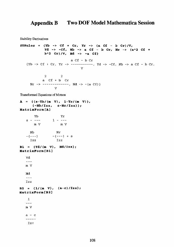
Appendix B Two DOFModelMathematica Session
Stability Derivatives
SDRules = {Yb -> Cf + Cr, Yr -> (a Cf - b Cr)/V#
Yd -> -Cf, Nb -> a Cf - b Cr, Nr -> (aA2 Cf +
bA2 Cr)/V, Nd -> -a Cf}
a Cf - b Cr
{Yb -> Cf + Cr, Yr ->, Yd -> -Cf, Nb -> a Cf - b Cr,
V
2 2
a Cf + b Cr
Nr ->, Nd -> -(a Cf)}
V
Transformed Equations ofMotion
A = {{s-Yb/(m V), l-Yr/(m V)},
{-Nb/Izz, s-Nr/Izz}};
MatrixForm [A]
Yb Yr
s- 1
m V m V
Nb Nr
-(- ) -( ) + s
Izz Izz
Bl = {Yd/(m V), Nd/Izz};
MatrixForm [Bl]
Yd
m V
Nd
Izz
B2 = {l/(m V), (a-c)/Izz};
MatrixForm [B2]
1
m V
a- c
Izz
108

Appendix B TwoDOFModel Mathematica Session
B3 = {g/V, 0};
MatrixForm[B3]
g
v
B4 = {l/(m V), (a-d)/Izz>;
MatrixForm [B4]
m V
a - d
Izz
Transfer Function Denominator
Ds = Collect [Det [A] ,s]
Nb 2 Nr Yb Nr Yb Nb Yr
+ s + + s (-( ) )
Izz Izz m V Izz m V Izz m V
Transfer FunctionNumerators
Nbd =
Collect [Det [Transpose [Rep lacePart [Transpose [A],Bl,l]]],s]
Nd Nr Yd s Yd Nd Yr
Izz Izz m V m V Izz m V
Nba = Collect [Det [Transpose [ReplacePart [
Transpose [A],B2,l]]],s]
a c Nr s a Yr c Yr
Izz Izz Izz m V m V Izz m V Izz m V
Nbt = Collect [Det [Transpose [ReplacePart [
Transpose [A],B3,l]]],s]
g Nr g s
-( ) +
Izz V V
109

Appendix B Two DOFModelMathematica Session
Nrd = Collect [Det [Transpose [ReplacePart [
Transpose [A] , Bl, 2 ] ] ] , s]
Nd s Nd Yb Nb Yd
+
Izz Izz m V Izz m V
Nra = Collect [Det [Transpose [ReplacePart [
Transpose [A],B2,2]]],s]
a c Nb a Yb c Yb
Izz Izz Izz m V Izz m V Izz m V
Nrt = Collect [Det [Transpose [ReplacePart [
Transpose [A] , B3 , 2] ] ] , s]
g Nb
Izz V
Nrn = Collect [Det [Transpose [ReplacePart [
Transpose [A] ,B4,2] ] ] , s]
ad Nb a Yb d Yb
Izz Izz Izz m V Izz m V Izz m V
Transfer Functions
Sideslip Angle
Gbd = Nbd/Ds
Nd Nr Yd s Yd Nd Yr
Izz Izz m V m V Izz m V
Nb 2 Nr Yb Nr Yb Nb Yr
+ s + + s (-( ) )
Izz Izz m V Izz m V Izz m V
Gba = Nba/Ds
a c Nr s a Yr c Yr
Izz Izz Izz m V m V Izz m V Izz m V
Nb 2 Nr Yb Nr Yb Nb Yr
+ s + + s (-( ) )
Izz Izz m V Izz m V Izz m V
110
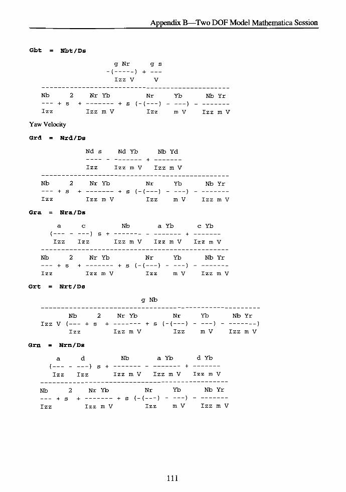
Appendix B Two DOFModelMathematica Session
Gbt = Nbt/Ds
g Nr g s
( ) +
Izz V V
Nb 2 Nr Yb Nr Yb Nb Yr
+ s + + s (-( ) )
Izz Izz m V Izz m V Izz m V
Yaw Velocity
Grd = Nrd/Ds
Nd s Nd Yb Nb Yd
+
Izz Izz m V Izz m V
Nb 2 Nr Yb Nr Yb Nb Yr
+ s + + s (-( ) )
Izz Izz m V Izz m V Izz m V
Gra = Nra/Ds
a c Nb a Yb c Yb
Izz Izz Izz m V Izz m V Izz m V
Nb 2 Nr Yb Nr Yb Nb Yr
+ s + + s (-( ) )
Izz Izz m V Izz m V Izz m V
Grt = Nrt/Ds
g Nb
Nb 2 Nr Yb Nr Yb Nb Yr
Izz V ( + s + + s (-( ) ) )
Izz Izz m V Izz m V Izz m V
Grn = Nrn/Ds
ad Nb a Yb d Yb
Izz Izz Izz m V Izz m V Izz m V
Nb 2 Nr Yb Nr Yb Nb Yr
+ s + + s (-( ) )
Izz Izz m V Izz m V Izz m V
111

Appendix B Two DOFModelMathematica Session
Steady State Step-Input Response Gains
SideslipAngle
Sbd = Simplify [Limit [Gbd, s->0] ]
-(m Nd V)- Nr Yd + Nd Yr
m Nb V + Nr Yb - Nb Yr
Sba = Simplify [Limit [Gba, s->0] ]
-Nr -amV+cmV+aYr-cYr
m Nb V + Nr Yb - Nb Yr
Sbt = Simplify [Limit [Gbt, s->0]]
g m Nr
_( )
m Nb V + Nr Yb - Nb Yr
Yaw Velocity
Srd = Simplify [Limit [Grd, s->0]]
-(Nd Yb) + Nb Yd
m Nb V + Nr Yb - Nb Yr
Sra = Simplify [Limit [Gra, s->0] ]
Nb -
a Yb + c Yb
m Nb V + Nr Yb - Nb Yr
Srt = Simplify [Limit [Grt, s->0] ]
g m Nb
m Nb V + Nr Yb - Nb Yr
Srn = Simplify [Limit [Grn, s->0] ]
Nb - a Yb + d Yb
m Nb V + Nr Yb - Nb Yr
Front Tire Slip Angle
Safd = Simplify [Sbd + a/V Srd - 1]
2 2
(m Nb V + m Nd V + a Nd Yb + Nr V Yb - a Nb Yd + Nr V Yd
Nb V Yr - Nd V Yr) / (V (-(m Nb V)- Nr Yb + Nb Yr) )
112

Appendix B Two DOFModelMathematica Session
Safa = Simplify [Sba + a/V Sra]
2 2 2
(- (a Nb) +NrV+amV -cmV +a Yb-acYb-aVYr+
c V Yr) / (V (-(m Nb V)- Nr Yb + Nb Yr) )
Saft = Simplify [Sbt + a/V Srt]
g m (a Nb - Nr V)
V (m Nb V + Nr Yb - Nb Yr)
Rear Tire Slip Angle
Sard = Simplify [Sbd - b/V Srd]
2
m Nd V - b Nd Yb + b Nb Yd + Nr V Yd - Nd V Yr
V (-(m Nb V)- Nr Yb + Nb Yr)
Sara = Simplify [Sba- b/V Sra]
2 2
(bNb + NrV + amV -cmV -abYb + bcYb-aVYr +
c V Yr) / (V (-(m Nb V)- Nr Yb + Nb Yr) )
Sart = Simplify [Sbt- b/V Srt]
g m (b Nb + Nr V)
V (-(m Nb V)- Nr Yb + Nb Yr)
Path Curvature
Scd = Simplify[l/V Srd]
- (Nd Yb) + Nb Yd
V (m Nb V + Nr Yb - Nb Yr)
Sea = Simplify [1/V Sra]
Nb -
a Yb + c Yb
V (m Nb V + Nr Yb - Nb Yr)
Set = Simplify[l/V Srt]
g m Nb
V (m Nb V + Nr Yb - Nb Yr)
113

AppendixBTwo DOFModelMathematica Session
Lateral Acceleration
SAd = Simplify [V/g Srd]
V (-(Nd Yb) + Nb Yd)
g (m Nb V + Nr Yb - Nb Yr)
SAa = Simplify [V/g Sra]
V (Nb -
a Yb + c Yb)
g (m Nb V + Nr Yb - Nb Yr)
SAt = Simplify [V/g Srt]
m Nb V
m Nb V + Nr Yb - Nb Yr
Steer Angle Response to Path Radius
deltaR = delta /. Solve[Scd == 1/R / delta, delta] [ [1, 1] ]
2
- (m Nb V ) - Nr V Yb + Nb V Yr
_( )
-(Nd R Yb) + Nb R Yd
Terml = Coefficient [Expand [deltaR] ,V, 2] VA2
2
m Nb V
-(Nd R Yb) + Nb R Yd
TermlS = Simplify [Terml /. SDRules]
2
(a Cf - b Cr) m V
a Cf Cr R + b Cf Cr R
TermlSa = Numerator [TermlS] / Simplify [Denominator [
TermlS] /. a->L-b]
2
(a Cf - b Cr) m V
Cf Cr L R
114

Appendix B TwoDOFModelMathematica Session
Terms 2 3 = ExpandNumerator [Simplify [Coefficient [Expand [
deltaR], V] V]]
-(Nr V Yb) + Nb V Yr
Nd R Yb - Nb R Yd
Terms23S = Simplify [Terms23 /. SDRules /. a->L-b]
L
R
deltaRl = Terml + Terms23S
2
L m Nb V
- +
R - (Nd R Yb) + Nb R Yd
deltaR2 = TermlSa + Terms23S
2
L (a Cf - b Cr) m V
- +
R Cf Cr L R
UndersteerGradient
Kus = Coefficient [Simplify [deltaRl R g] ,VA2]
g m Nb
-(Nd Yb) + Nb Yd
Kusl = Simplify [Kus /. SDRules]
(a Cf - b Cr) g m
(a + b) Cf Cr
Stability Factor
Kl = Simplify [K /. Solve [Srd == V/(L (1+K VA2)), K][[l]]]
2
m Nb V + L Nd Yb + Nr V Yb - L Nb Yd - Nb V Yr
2
L V (-(Nd Yb) + Nb Yd)
115

Appendix B Two DOFModelMathematica Session
K2 = Simplify [Numerator [Kl]- Coefficient [Numerator [Kl] ,
VA2] VA2 /. SDRules /. a->L-b] + Coefficient [
Numerator [Kl] , VA2] VA2 / Denominator [Kl]
m Nb
L (-(Nd Yb) + Nb Yd)
K3 = Simplify [K2 /. SDRules]
(a Cf - b Cr) m
a Cf Cr L + b Cf Cr L
K4 = Numerator [K3] /Simplify[ (Denominator [K3] /,
a -> L - b)]
(a Cf - b Cr) m
2
Cf Cr L
Neutral Steer Point
dl = Simplify [d /.
Nb
a - --
Yb
d2 = Simplify [dl /,
(a + b) Cr
Solve [Numerator [Srn] == 0, d] [ [1] ] ]
SDRules]
Cf + Cr
d3 = Simplify [d2 /. a
Cr L
> L b]
a)/L
Cf + Cr
Static Margin
SM = (dl
Nb
-( )
L Yb
SMI = Simplify [SM /.
-(a Cf) + b Cr
Cf L + Cr L
SDRules]
116

Appendix B Two DOFModelMathematica Session
Tangent Speed
Vtan = v /. Solve[Sbd deltaR == 0,V][[2,1]]
Nr Yd - Nd Yr
-( )
m Nd
Vtanl = Sqrt [Simplify [Expand[ (V /. Solve [V == Simplify [
Vtan /. SDRules] ,V] [ [2,1] ]) A2] ] ]
b (a + b) Cr
Sqrt[-( )]
a m
Vtan2 = Sqrt [Simplify [Numerator [VtanlA2] /. a -> L-b] /
Denominator [Vtanl A 2 ] ]
b Cr L
Sqrt[-( )]
a m
Critical Speed
Vcrit = v /. Solve [Denominator [Srd] == 0,V][[1]]
Nr Yb - Nb Yr
-( )
m Nb
Vcritl = Sqrt [Simplify [ (V /. Solve [V == Vcrit /
SDRules,V] [[2,1]])A2]]
2
(a + b) Cf Cr
Sqrt [ ]- (a Cf m) + b Cr m
Vcrit2 = Sqrt [Simplify [Numerator [VcritlA2] /. a -> L-b]/
Denominator [Vcritl A2] ]
2
Cf Cr L
Sqrt [ ]
- (a Cf m) + b Cr m
Characteristic Speed
Vchar = v /. Solve[deltaR == 2 L/R, V] [ [2, 1] ]
(-(Nr Yb) + Nb Yr + Sqrt [-4 LmNb (2 Nd Yb - 2 Nb Yd) +
2
(Nr Yb - Nb Yr) ]) / (2 m Nb)
117

Appendix B Two DOFModelMathematica Session
Vcharl = Sqrt [Simplify [ (V /. Solve [V == Vchar /-
SDRules, V] [[2,1]])A2]]
(a + b) Cf Cr (a + b - 2 L)
Sqrt[ ]
-(a Cf m) + b Cr m
Vchar2 = Sqrt [Simplify [Numerator [VcharlA2] /. a -> L-b]/
Denominator [Vcharl A2] ]
2
Cf Cr L
Sqrt[-( )]
-(a Cf m) + b Cr m
Yaw Radius ofGyration
kz = Sqrt[Izz/m]
Izz
Sqrt[ ]
m
Geometry to Inertia Ratio
GIR = LA2/kzA2
2
L m
Izz
Total Cornering Factor
TCF = Cf Cr/mA2
Cf Cr
2
m
Characteristic Equation
Ds == 0
Nb 2 Nr Yb Nr Yb Nb Yr
+ s + + s (-( ) ) == 0
Izz Izz m V Izz m V Izz m V
a2 = Coefficient [Ds, sA2]
1
118

AppendixB Two DOFModel Mathematica Session
al = Coef ficient [Ds, s]
Nr Yb
-( )
Izz m V
aO = Ds - a2 sA2 - al s
Nb Nr Yb Nb Yr
+ _
Izz Izz m V Izz m V
UndampedNatural Frequency
wn = Simplify [Sqrt [aO ] ]
in Nb V + Nr Yb - Nb Yr
Sqrt[ ]
Izz m V
wnl = Simplify [wn /. SDRules]
2 2 2 2
a Cf Cr + 2 a b Cf Cr + b Cf Cr + a Cf m V - b Cr m V
Sqrt[ ]
2
Izz m V
Damping Ratio
zeta = Simplify [al Izz m V/(2 Sqrt[wnA2 (Izz m V)A2])]
- (m Nr V + Izz Yb)
2 Sqrt [Izz mV (hi Nb V + Nr Yb - Nb Yr) ]
zetal = Simplify [zeta /. SDRules]
2 2
-(Cf Izz + Cr Izz + a Cf m + b Cr m) /
2 2 2
(2 Sqrt [Izz m (a Cf Cr + 2 a b Cf Cr + b Cf Cr + a Cf m V -
2
b Cr m V ) ] )
119

Appendix B Two DOFModel Mathematica Session
Poles
poles = Solve [Ds==0, s] ;
si = s /- poles [[1,1]]
2
(m Nr V + Izz Yb - Sqrt[(-(m Nr V) - Izz Yb) -
4 Izz m V (m Nb V + Nr Yb - Nb Yr) ] ) / (2 Izz m V)
sla = Simplify [si /. SDRules]
2 2
( (Cf + Cr) Izz + (a Cf + b Cr) m-
2 2 2
Sqrt[(-(Cf Izz) - Cr Izz -
a Cf m - b Cr m)-
2 2 2
4 Izz m (a Cf Cr + 2 a b Cf Cr + b Cf Cr + a Cf m V -
2
b Cr m V ) ] ) / (2 Izz m V)
s2 = s /. poles [[2,1]]
2
(m Nr V + Izz Yb + Sqrt[(-(m Nr V) - Izz Yb)
4 Izz m V (m Nb V + Nr Yb - Nb Yr) ] ) / (2 Izz m V)
s2a = Simplify [s2 /. SDRules]
2 2
( (Cf + Cr) Izz + (a Cf + b Cr) m +
2 2 2
Sqrt[(-(Cf Izz) - Cr Izz -
a Cf m- b Cr m)
2 2 2
4 Izz m (a Cf Cr + 2 a b Cf Cr + b Cf Cr + a Cf m V -
2
b Cr m V ) ] ) / (2 Izz m V)
Zeros
Zbd = s /. Solve [Nbd == 0, s][[l,l]]
- (m Nd V) - Nr Yd + Nd Yr
_( }
Izz Yd
120

Appendix B Two DOFModelMathematica Session
Zbdl = Simplify [Zbd /. SDRules]
2 2
abCr+b Cr+amV
Izz V
Zba = s /. Solve [Nba == 0, s][[l,l]]
-Nr -amV+cmV+aYr-cYr
_( )
Izz
Zbal = Simplify [Zba /. SDRules]
2 2 2
acCf+abCr+b Cr-bcCr+amV -cmV
Izz V
Zbt = s /. Solve [Nbt == 0, s][[l,l]]
Nr
Izz
Zbtl = Simplify [Zbt /. SDRules]
2 2
a Cf + b Cr
Izz V
Zrd = s /. Solve [Nrd == 0, s][[l,l]]
- (Nd Yb) + Nb Yd
_( )
m Nd V
Zrdl = Simplify [Zrd /- SDRules]
(a + b) Cr
a m V
Zra = s /. Solve [Nra == 0, s][[l,l]]
Nb -
a Yb + c Yb
-( )
(a -
c) m V
Zral = Simplify [Zra /. SDRules]
-(c Cf) + a Cr + b Cr -
c Cr
a m V -
c m V
121

Appendix B TwoDOFModelMathematica Session
Zrt = Solve [Nrt == 0, s]
{{}}
122

Appendix C Two DOF ModelMATLAB Programs
C.l DOF2Control.m
%DOF2Control 2 DOF Model Execution Control
%
Controls execution of 2 DOF model. Sets control input type (step, step
ramp, ramp step / ramp down, or sine steer) . Sets simulation parameters.
% Created 1/11/96
% J. Kiefer
% Control Input Type
step= 1;
ramp = 2;
rampsquare = 3;
sine = 4;
% Step steer
% Ramp step steer
% Ramp square steer
% Sine steer
input = 1; % Select which control input to use
% Simulation Parameters
tO = 0.0; % s
tr = 0.2; % s
td = 1.0; % s
ts = 1.0; % s
tf = 4.0; % s
tol = le-5; %
Initial time for steer input
Ramp time
EWell time
Period for sine steer
Final time for simulation
Simulation accuracy (default = le-3)
123

AppendixCTwoDOFModel MATLAB Programs
C.2 DOF2Param.m
%DOF2Param 2 DOF Model Independent Parameters and Simulation Control
%
Sets independendent vehicle, tire, control, and disturbance parameters
for 2 DOF model.
% Created 1/7/96
% J. Kiefer
% Initialization
clear all;
clc;
global m Izz L a b c u Cf Cr dO Fzf Fzr Fyg Fya tO tr td ts tf input;
global Bl CI Dl El B3 C3 B5 C5;
% Constants
g = 9.81; % m/s~2
% Vehicle Independent Parameters
m = 1775; % kg
Izz = 1960; % kg-m^2
f = 0.52; %
L = 2.372; % m
u = 100; % km/hr
% Control and Disturbance Inputs
dO == 1; % deg
theta = 0; % deg
Fya = 0; % N
c = 1.25; % m
%
% Linear Tire Model Parameters
Cf ==-1230.5; % N/deg
Cr ==-1155.5; % N/deg
Acceleration due to gravity
Gross vehicle mass
Yaw inertia
Fraction of weight on front axle
Wheelbase
Vehicle forward speed
Steer input magnitude
Side slope
Aerodynamic side force
Distance from front axle to
aerodynamic side force
Front cornering stiffness (one tire)
Rear cornering stiffness (one tire)
% Non Linear Tire Model Parameters
% Normalized Lateral Force Magic Formula Parameters
Bl = 0.5835;
CI = 1.7166
Dl = 1.0005
El = 0.2517
% Cornering Coefficient Parameters
B3 = 0.333;
C3 =-1.352e-5;
% Friction Coefficient Parameters
B5 = 1.173;
C5 = -3.696e-5;
% Unit Conversions
u = u*1000/3600; % m/s Vehicle forward speed
124

AppendixCTwo DOFModelMATLAB Programs
dO = d0*pi/180; % rad Step steer input
Cf = Cf*180/pi*2; % N/rad Front tire cornering stiffness (two tires)
Cr = Cr*180/pi*2; % N/rad Rear tire cornering stiffness (two tires)
125

AppendixCTwo DOFModel MATLAB Programs
C.3 DOF2DependParam.m
%DOF2DependParam 2 DOF Model Dependent Parameter Calculation
%
% Calculates values of dependent parameters for 2 DOF model.
%
% Created 1/7/96
% J. Kiefer
% Dependent Parameters
a = (l-f)*L;
b = f*L;
V = u;
Fyg = m*g*sin(theta*pi/180) ;
Fzf = m*g*f/2*cos(theta*pi/180);
Fzr = m*g*(l-f)/2*cos(theta*pi/180);
% Stability Derivatives
Yb = Cf + Cr;
Yr = (a*Cf-b*Cr) /V;
Yd = -Cf ;
Nb = a*Cf-b*Cr;
Nr = (a~2*Cf+b~2*Cr) /V;
Nd = -a*Cf ;
% m Distance from front tire to C.G.
% m Distance from rear tire to C.G.
% m/s Vehicle speed
% N Side slope lateral force
% N Front tire normal load (one tire)
% N Rear tire normal load (one tire)
% N/rad Damping-in-sideslip
% N-s/rad Lateral force / yaw coupling
% N/rad Control force
% N-m/rad Directional stability
% N-m-s/rad Yaw damping
% N-m/rad Control moment
126

AppendixCTwo DOFModel MATLAB Programs
C.4 SteerAngle.m
function delta = SteerAngle (t, input, t0,tr,td,ts,tf ,d0)
%SteerAngle Calculate Steer Angle Based on Time and Control Input Selection
%
%delta = SteerAngle (t, input, tO, tr,td,ts,tf,dO)
%
% Determines steer angle based on current time, input selection, and
% simulation parameters. Input selection may be step, ramp, ramp square, or
% sine. Called by functions D0F2LDE.m, D0F2NLDE.m, D0F3LDE.m, D0F3NLDE.m.
%
% Inputs:
% t Time (s)
% input Flag for input selection
% 1 =step
% 2 =ramp
% 3 = rampsquare
% 4 = sine
% to Initial time for simulation (s)
% tr Ramp time (s)
% td EWell time (s)
% ts Period for sine steer (s)
% tf Final time for simulation (s)
%
%
%
dO Steer input magnitude (rad)
Outputs:
%
%
%
delta Steer angle (rad)
Created 1/7/96
% J. Kiefer
% Crash Through Result
delta = 0;
% Step Steer
if input == 1
delta = dO;
if t < tO
delta
end
end
0;
% Ramp Step Steer
if input == 2
delta = dO;
if t < tO + tr
delta = d0*(t-t0)/tr;
end
if t < tO
delta = 0;
end
end
% Ramp Square Steer
if input == 3
127

AppendixCTwo DOFModelMATLAB Programs
delta = 0;
if t < tO + 2*tr + td
delta = d0*(t0+td+2*tr-t)/tr;
end
if t < tO + tr + td
delta = dO;
end
if t < tO + tr
delta = d0*(t-t0)/tr;
end
if t < tO
delta = 0;
end
end
% Sine Steer
if input == 4
delta = d0*sin(2*pi*(t-t0)/ts) ;
if t < tO
delta = 0;
end
end
128

AppendixCTwo DOFModelMATLAB Programs
C.5 DOF2LFreq.m
%DOF2LFreq Frequency Response of Linear 2 DOF Model
% For a Single Set of Parameters
%
% Generates bode plot data for linear 2 DOF model for outputs of
% sideslip angle and yaw speed, and for inputs of steer angle control,
% aerodynamic side force disturbance, and road side slope disturbance.
%
% Created 2/4/96
% J. Kiefer
D0F2Param; % Set independent parameters
D0F2Control ; % Set execution control parameters
D0F2DependParam; % Calculate dependent parameters
% Transfer Function Denominator
D = [1 -Nr/Izz-Yb/ (m*V) Nb/Izz+(Nr*Yb-Nb*Yr) / (Izz*m*V) ] ;
% Transfer Function Numerators
Nbd = [Yd/(m*V) (Nd*Yr-Nr*Yd-Nd*m*V) / (Izz*m*V) ] ;
Nba = [1/ (m*V) (c-a) /Izz+ ( (a-c) *Yr-Nr) / (Izz*m*V) ] ;
Nbt = [g/V -g*Nr/(Izz*V)] ;
Nrd = [Nd/Izz (Nb*Yd-Nd*Yb) / (Izz*m*V) ] ;
Nra = [(a-c) /Izz ( (c-a)*Yb+Nb) / (Izz*m*V) ] ;
Nrt = [g*Nb/ (Izz*V) ] ;
% Bode Plot Data
w = lcgspace(-l,2) *2*pi;
[Mbd,Pbd,w] = bode (Nbd,D,w) ;
[Mba,Pba,w] = bode (Nba,D,w) ;
[Mbt,Pbt,w] = bode (Nbt,D,w) ;
[Mrd,Prd,w] = bode (Nrd,D,w) ;
[Mra,Pra,w] = bode (Nra,D,w) ;
[Mrt,Prt,w] = bode (Nrt,D,w);
129
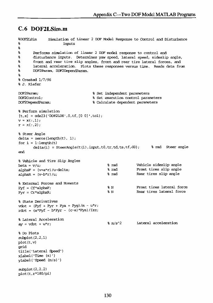
AppendixCTwo DOFModel MATLAB Programs
C.6 DOF2LSim.m
%D0F2LSim Simulation of Linear 2 DOF Model Response to Control and Disturbance
% Inputs
%
% Performs simulation of linear 2 DOF model response to control and
% disturbance inputs. Determines yaw speed, lateral speed, sideslip angle,
% front and rear tire slip angles, front and rear tire lateral forces, and
% lateral acceleration. Plots these responses versus time. Reads data from
% D0F2Param, D0F2DependParam.
%
% Created 1/7/96
% J. Kiefer
D0F2Param;
D0F2Control;
D0F2DependParam;
% Set independent parameters
% Set execution control parameters
% Calculate dependent parameters
% Perform simulation
[t,x] = ode23(,DOF2LDE',0,tf, [0 0]',tol);
v = x(:,l) ;
r = x(:,2);
% Steer Angle
delta = zeros ( length (t) , 1) ;
for i = l:length(t)
delta(i) = SteerAngle (t (i) , input, t0,tr,td,ts,tf, dO) ;
end
% rad Steer angle
% Vehicle and Tire Slip Angles
beta = v/u;
alphaF = (v+a*r) /u-delta;
alphaR = (v-b*r)/u;
% rad
% rad
% rad
Vehicle sideslip angle
Front tires slip angle
Rear tires slip angle
% External Forces and Moments
Fyf = Cf*alphaF;
Fyr = Cr*alphaR;
% N
% N
Front tires lateral force
Rear tires lateral force
% State Derivatives
vdot = (Fyf + Fyr + Fya + Fyg) /m-
u*r;
rdot = (a*Fyf - b*Fyr - (c-a) *Fya) /Izz;
% Lateral Acceleration
ay= vdot + u*r;
% m/s^ Lateral acceleration
% Do Plots
subplot (2, 2,1)
plot(t,v)
grid
title ('Lateral Speed
'
)
xlabeK'Time (s) ')
ylabel('Speed (m/s) ')
subplot (2, 2, 2)
plot(t,r*180/pi)
130

AppendixCTwo DOFModel MATLAB Programs
grid
title ('Yaw Speed')
xlabelCTime (s) ')
ylabel( 'Speed (deg/s)'
)
subplot (2, 2, 3)
plot(t,beta*180/pi,t,alphaF*180/pi, ,t,alphaR*180/pi,'-.
'
,t,delta*180/pi,
'
:'
)
grid
title ( 'Vehicle Sideslip Angle, Tire Slip Angles, Steer Angle')
xlabeK 'Time (s)'
)
ylabel ('
Slip Angle (deg)'
)
subplot (2, 2, 4)
plot(t,ay/g)
grid
title ('
Lateral Acceleration'
)
xlabel( 'Time (s) ')
ylabel ( 'Acceleration (g)'
)
131

AppendixCTwo DOFModel MATLAB Programs
C.7 DOF2LDE.m
function xdot = DOF2NLDE(t,x)
%DOF2NLDE Non Linear Differential Equations for 2 DOF Model
%
%xdot = D0F2NLDE(t,x)
%
% Determines derivatives of lateral speed and yaw speed given time and
% state vector. Non linear tire and non linear slip angles. Used with ode23
% for simulation.
% Inputs:
% t
% x(l)
% x(2)
% Outputs:
% xdot(l)
% xdot (2)
%
% Created 2/18/96
% J. Kiefer
Time (s)
Lateral speed (m/s)
Yaw speed (rad/s)
Derivative of lateral speed (m/s^2)
Derivative of yaw speed (rad/s''2)
global m Izz L a b c u dO Fzf Fzr Fyg Fya tO tr td ts tf input;
delta = SteerAngle(t, input, tO, tr,td,ts,tf,dO);
alphaF = atan( (x(l)+a*x(2) ) /u) -delta;
alphaR = atan( (x(l)-b*x(2) )/u) ;
[Fyf, Mzf] = NLTire(Fzf, alphaF);
[Fyr, Mzr] = NLTire(Fzr, alphaR);
xdot = [-u*x(2) + (2*Fyf*cos (delta) +2*Fyr+Fya+Fyg)/m
(2*a*Fyf*cos (delta) -2*b*Fyr+ (a-c) *Fya) /Izz] ;
132

Appendix C Two DOFModelMATLAB Programs
C.8 DOF2NLSim.m
%DOF2NLSim Simulation of Non-Linear 2 DOF Model Response to Control and Disturbance
% Inputs
%
% Performs simulation of non linear 2 DOF model response to control and
% disturbance inputs. Determines yaw speed, lateral speed, sideslip angle,
% front and rear tire slip angles, front and rear tire lateral forces, and
% lateral acceleration. Plots these responses versus time. Reads data from
% D0F2Param, D0F2DependParam.
%
% Created 2/18/96
% J. Kiefer
D0F2Param; % Set independent parameters
D0F2Control; % Set execution control parameters
D0F2DependParam; % Calculate dependent parameters
% Perform simulation
[t,x] = ode23(,DOF2NLDE',0,tf, [0 0]',tol);
v = x(:,l) ;
r = x(:,2) ;
% Steer Angle
delta = zeros (length(t) , 1) ;
for i = l:length(t)
delta(i) = SteerAngle (t(i) , input, tO,tr,td,ts,tf ,d0) ; % rad Steer angle
end
% Vehicle and Tire Slip Angles
beta = atan(v/u) ; % rad Vehicle sideslip angle
alphaF = atan( (v+a*r) /u) -delta; % rad Front tires slip angle
alphaR = atan( (v-b*r) /u) ; % rad Rear tires slip angle
% External Forces and Moments
Fyf = NLTire(Fzf, alphaF); % N Front tire lateral force (one tire)
Fyr = NLTire(Fzr, alphaR) ; % N Rear tire lateral force (one tire)
% State Derivatives
vdot = (2*Fyf.*cos (delta) + 2*Fyr + Fya + Fyg) /m-
u*r;
rdot = (2*a*Fyf.*cos (delta)- 2*b*Fyr - (c-a)*Fya)/Izz;
% Lateral Acceleration
ay= vdot + u*r;
% m/s^2 Lateral acceleration
% Do Plots
subplot(2,2,l)
plot(t,v)
grid
title('Lateral Speed')
xlabeK'Time (s) ')
ylabel ('Speed (m/s) ')
subplot (2, 2, 2)
plot(t,r*180/pi)
133

AppendixCTwo DOFModel MATLAB Programs
grid
title ('Yaw Speed')
xlabelCTime (s) ')
ylabel ('
Speed (deg/s)'
)
subplot (2, 2, 3)
plot(t,beta*180/pi,t,alphaF*180/pi,' '
,t,alphaR*180/pi, '-.'
,t,delta*180/pi,
'
: ')
grid
title ( 'Vehicle Sideslip Angle, Tire Slip Angles, Steer Angle')
xlabel( 'Time (s) ')
ylabel ('
Slip Angle (deg)'
)
subplot (2, 2, 4)
plot (t,ay/g)
grid
title ('
Lateral Acceleration'
)
xlabel( 'Time (s)'
)
ylabel ( 'Acceleration (g)'
)
134

AppendixCTwo DOFModel MATLAB Programs
C.9 DOF2NLDE.m
function xdot = D0F2NLDE(t,x)
%D0F2NLDE Non Linear Differential Equations for 2 DOF Model
%
%xdot = D0F2NLDE(t,x)
%
% Determines derivatives of lateral speed and yaw speed given time and
% state vector. Non linear tire and non linear slip angles. Used with ode23
% for simulation.
%
% Inputs:
% t Time (s)
% x(l) Lateral speed (m/s)% x(2) Yaw speed (rad/s)% Outputs:
% xdot(l) Derivative of lateral speed (m/s^2)% xdot (2) Derivative of yaw speed (rad/sA2)%
% Created 2/18/96
% J. Kiefer
global m Izz L a b c u dO Fzf Fzr Fyg Fya tO tr td ts tf input;
delta = SteerAngle(t, input, tO, tr,td,ts,tf,dO);alphaF =
atan((x(l)+a*x(2))/u)-delta;
alphaR = atan( (x(l)-b*x(2) )/u) ;
Fyf = NLTire(Fzf, alphaF);
Fyr = NLTire(Fzr, alphaR);
xdot = [-u*x(2) + (2*Fyf*cos (delta) +2*Fyr+Fya+Fyg)/m
(2*a*Fyf*cos (delta) -2*b*Fyr+ (a-c) *Fya) /Izz] ;
135

Appendix D RelevantLiterature
"Control ofVehicleDynamics."
Automotive Engineering,May 1995, p. 87-93.
"Road Vehicles - Lateral Transient Response TestMethods."
ISO 7401,May 1988.
"Road Vehicles - Steady State Circular TestProcedure."
ISO 4138, Aug. 1982.
"Road Vehicles - Vehicle Dynamics and Road-Holding Ability -
Vocabulary."
ISO 8855,Dec. 1991.
"Vehicle DynamicsTerminology."
SAE J670e,Warrendale, PA: SAE, 1976.
1994Motor Sports Engineering Conference Proceedings: Volume 1: Vehicle Design
Issues. SAE Publication No. P-287, Dec. 1994.
Allen, R. Wade and Theodore J. Rosenthal. "A Computer Simulation Analysis of SafetyCritical Maneuvers for Assessing Ground Vehicle Dynamic
Stability."
SAE Paper
No. 930760, Mar. 1993.
Allen, R. Wade and Theodore J. Rosenthal. "Requirements for Vehicle Dynamics
SimulationModels."
SAE Paper No. 940175, Feb. 1994.
Allen, R. Wade, Raymond E. Magdaleno, Theodore J. Rosenthal, David H. Klyde, and
Jeffrey R. Hogue. 'TireModeling Requirements for Vehicle DynamicsSimulation."
SAE Paper No. 950312, Feb. 1995.
Allen, R.Wade, Thomas T. Myers, and Theodore J. Rosenthal. "Vehicle StabilityConsiderations with Automatic and FourWheel Steering
Systems."
SAE Paper No.
931979, Nov. 1993.
Allen, R. Wade, Theodore J. Rosenthal, and Jeffrey R. Hogue. "Modeling and Simulation
ofDriverA^ehicleInteraction."
SAE PaperNo. 960177, Feb. 1996.
Allen, R. Wade, Theodore J. Rosenthal, and Henry T. Szostak. "Steady State and
Transient Analysis ofGround VehicleHandling."
SAE Paper No. 870495, 1987.
Allen, R. Wade, Theodore J. Rosenthal, David H. Klyde, Keith J. Owens, and Henry T.
Szostak. "Validation ofGround Vehicle Computer Simulations Developed for
Dynamics StabilityAnalysis."
SAE Paper No. 920054, Feb. 1992.
Allen, R.Wade, Henry T. Szostak, Theodore J. Rosenthal, David H. Klyde, and Keith J.
Owens. "Characteristics Influencing Ground Vehicle Lateral/DirectionalDynamicStability."
SAE Paper No. 910234, Feb. 1991.
Antoun, R.J, P.B. Hackert, M.C. O'Leary, and A. Sitchin. "Vehicle Dynamic HandlingComputer Simulation -- Model Development, Correlation, and Application UsingADAMS."
SAE Paper No. 860574, 1986.
Araki, Kazuo and Hideo Sakai. "Study ofTireModel Consisting ofTheoretical and
Experimental Equations for Vehicle Dynamics Analysis- Part 2: Under the
Condition ofVarious Velocity on the Asphaltic RoadSurface."
SAE PaperNo.
960996, Feb. 1996.
Ashley, Steven. "Spin Control forCars."
Mechanical Engineering, Vol. 117, No. 6, June
1995, p. 66-68.
136

Appendix D Relevant Literature
Bakker, Egbert, Lars Nyborg, and Hans B. Pacejka. 'TyreModelling for Use in Vehicle
DynamicsStudies."
SAE Paper No. 870421, 1987.
Bakker, Egbert, Hans B. Pacejka, and Lars Lidner. "A New Tire Model with an
Application in Vehicle DynamicsStudies."
SAE Paper No. 890087, 1989.
Barak, Pinhas. "Magic Numbers in Design of Suspensions for PassengerCars."
SAE
Paper No. 911921, 1991.
Barbieri, Nilson. "SuspensionsOptimization."
SAE Paper No. 921491, 1992.
Bastow, D. and G. Howard. Car Suspension andHandling. Warrendale, PA: SAE, 1993.
Bernard, James E. and C.L. Clover. 'TireModeling for Low-Speed and High-SpeedCalculations."
SAE Paper No. 950311, Feb. 1995.
Bernard, James E. and C.L. Clover. "Validation ofComputer Simulations ofVehicleDynamics."
SAE Paper No. 940231, Feb. 1994.
Bixel, Ronald A., Gary J. Heydinger, N.J. Durisek, and Dennis A. Guenther. "New
Developments in Vehicle Center ofGravity and Inertial Parameter Estimation andMeasurement."
SAE Paper No. 950356, Feb. 1995.
Blank,Matthew and Donald Margolis. "The Effect ofNormal Force Variation on the
Lateral Dynamics ofAutomobiles."
SAE Paper No. 960484, Feb. 1996.
Bowman, J. Eric and E.H. Law. "A Feasibility Study of an Automotive Slip Control
BrakingSystem."
SAE Paper No. 930762, Mar. 1993.
Breuer, Bert, Thomas Bachmann, Stefan Ernesti, and Jorg Stocker. "Methods and
Instruments for On-BoardMeasurement ofTyre/RoadFriction."
SAE Paper No.
942470, Dec. 1994.
Bundorf, R.T. and R.L. Leffert. 'The Cornering Compliance Concept for Description of
Vehicle Directional ControlProperties."
SAE Paper No. 760713, Oct. 1976.
Cambiaghi, Danilo andMarco Gadola. "Computer-Aided Racing CarDesign and
Development at the University ofBrescia,Italy."
SAE Paper No. 942507, Dec.
1994.
Captain, K.M., A.B. Boghani, and D.N. Wormley. "Analytical TireModels for Dynamic
VehicleSimulation."
Vehicle System Dynamics, Vol. 8, 1979, p. 1-32.
Car Suspension Systems and Vehicle Dynamics. SAE Publication No. SP-878, Sept.
1991.
Chen H Fred and Dennis A. Guenther. "The Effects of Suspension Stiffness on HandlingResponses."
SAE Paper No. 911928, 1991.
Chocholek, S.E. "The Development of a Differential for theImprovement ofTraction
Control."
IMechE Paper No. C368/88, 1988.
Chrstos, Jeffrey P. "A Simplified Method for theMeasurement ofComposite Suspension
Parameters."
SAE Paper No. 910232, 1991.
Clover, Chris L. and James E. Bernard. "The Influence ofLateral Load Transfer
Distribution on DirectionalResponse."
SAE PaperNo. 930763, Mar. 1993.
Cole, D.E. Elementary Vehicle Dynamics. Ann Arbor, MI: University ofMichigan, 1972.
137

AppendixD RelevantLiterature
Crahan, Thomas C. "Modeling Steady-State Suspension Kinematics and Vehicle Dynamics
ofRoad Racing Cars- Part I: Theory and
Methodology."
SAE PaperNo. 942505,Dec. 1994.
Crahan, Thomas C. "Modeling Steady-State Suspension Kinematics andVehicle DynamicsofRoad Racing Cars
- Part II:Examples."
SAE Paper No. 942506, Dec. 1994.
Crolla, D.A. andM.B.A. Abdel-Hady. "Semi-Active Suspension Control for a Full
VehicleModel."
SAE Paper No. 91 1904, Sept. 1991.
Day, Terry D. "An Overview of the HVE VehicleModel."
SAE PaperNo. 950308, Feb.1995.
Dickison, J.G. and A.J. Yardley. "Development and Application of a Functional Model to
VehicleDevelopment."
SAE Paper No. 930835, Mar. 1993.
Dixon, John C. Tyres, Suspension andHandling, Cambridge, England: Cambridge
University Press, 1991.
Dreyer, Andreas and Heinz-DieterHeitzer. "Control Strategies for Active Chassis Systems
with Respect to RoadFriction."
SAE Paper No. 910660, Feb. 1991.
Egnaczak, Bernard C. "Supplement to: 'The Development of aDifferential for the
Improvement ofTractionControl."
Auto Tech 89, Session 5 Traction Control,Nov. 14, 1989.
ElBeheiry, ElSayed M. andDean C. Karnopp. "Optimization ofActive and Passive
Suspensions Based on a Full CarModel."
SAE Paper No. 951063, Feb. 1995.
Ellis, John R. Road Vehicle Dynamics, Akron, OH: J.R. Ellis, 1989.
Ellis, John R. Vehicle Dynamics. London: Business Books, 1969.
Floyd, R. Scott and E. Harry Law. "Simulation and Analysis of Suspension and
Aerodynamic Interactions ofRaceCars."
SAE Paper No. 942537, Dec. 1994.
Franklin, Gene F., J. David Powell, and Abbas Emami-Naeini. Feedback Control ofDynamic Systems. New York: Addison-Wesley Publishing Company, Inc., 1994.
Garrot,W. Riley, Douglas L. Wilson, and Richard A. Scott. "Digital Simulation for
AutomobileManeuvers."
Simulation, Sept. 1981, p. 83-91.
Gillespie, T.D. Fundamentals ofVehicle Dynamics. Warrendale, PA: SAE, 1992.
Gim, Gwanghun and Namcheol Kang. "Requirements of a Tire Model for Practical
Cornering Simulations ofVehicles."
SAE Paper No. 960179, Feb. 1996.
Gim, Gwanghun and Parviz E. Nikravesh. "A Three-Dimensional Tire Model for Steady-
State Simulations ofVehicles."
SAE Paper No. 931913, Nov. 1993.
Gim, Gwanghun and Parviz E. Nikravesh. "An AnalyticalModel ofPneumatic Tyres for
Vehicle Dynamic Simulations. Part 1: PureSlips."
International Journal ofVehicle
Design, Vol. 11, No. 6, 1990.
Gim, Gwanghun and Parviz E. Nikravesh. "An AnalyticalModel ofPneumatic Tyres for
VehicleDynamic Simulations. Part 2: ComprehensiveSlips."
International Journal
ofVehicle Design, Vol. 12, No. 1, 1991.
Gruening, James and James E. Bernard. "Verification ofVehicle Parameters for Use in
ComputerSimulation."
SAE Paper No. 960176, Feb. 1996.
138

Appendix D Relevant Literature
Gruening, James, Keith A. Williams, Kurt Hoffmeister, and James E. Bernard. 'TireForce andMoment
Processor."
SAE Paper No. 960182, Feb. 1996.
Guntur, R. and S. Sankar. "A Friction Circle Concept for Dugoff s Tyre FrictionModel."
International Journal ofVehicle Design, Vol. 1, No. 4, 1980.
Haney, Paul and JeffBraun. Inside Racing Technology. Redwood City, CA: TVMotorsports, 1995.
Heydinger, Gary J. "Improved Simulation and Validation ofRoad VehicleHandlingDynamics."
Ph.D. Dissertation, Ohio State University, Columbus, Ohio, 1990.
Heydinger, Gary J., W. Riley Garrot, and Jeffrey P. Chrstos. "The Importance ofTireLag on Simulated Transient Vehicle
Response."
SAE Paper No. 910235, 1991.
Heydinger, Gary J., Paul A. Grygier, and Seewoo Lee. "Pulse Testing TechniquesApplied to Vehicle Handling
Dynamics."
SAE PaperNo. 930828, Mar. 1993.
Holmes, H. and D. Alexander. Formula Car Technology. Santa Ana, CA: Steve Smith
Autosports, 1980.
Hopkins, Patrick and L. DanielMetz. "Oversteer/Understeer Characteristics of a LockedDifferential."
SAE Paper No. 942485, Dec. 1994.
Howard, Geoffrey. Chassis & Suspension Engineering, London, England: OspreyPublishing Limited, 1987.
Huang, Feng, J. Roger Chen, and Lung-Wen Tsai. "The Use ofRandom Steer Test Data
for Vehicle ParameterEstimation."
SAE Paper No. 930830,Mar. 1993.
Huchtkoetter, Heinrich and Heinz Klein. "The Effect ofVarious Limited-Slip Differentialsin Front-Wheel Drive Vehicles on Handling and
Traction."
SAE Paper No.
960717, Feb. 1996.
Ikushima, Y. and K Sawase. "A Study on the Effects of the Active YawMomentControl."
SAE Paper No. 950303, Feb. 1995.
Jung, Shinsub and Dennis A. Guenther. "An Examination of theManeuverability of an AllWheel Steer Vehicle at Low
Speed."
SAE Paper No. 910241, Feb. 1991.
Kaminaga, M., M. Murata, and Y. Tateishi. "FactoringNonlinear Kinematics into NewSuspension Design: A CAE Approach to Vehicle Roll
Dynamics."
SAE Paper No.
940871, Feb. 1994.
Karnopp, Dean. "Active Damping in Road Vehicle SuspensionSystems."
Vehicle System
Dynamics, Vol. 12, 1983, p. 291-316.
Kasprzak, James L. and R. Scott Floyd. "Use of Simulation to Tune Race CarDampers."
SAE Paper No. 942504, Dec. 1994.
Katz, Joseph. Race CarAerodynamics. Cambridge,MA: Robert Bentley, Inc., 1995.
Klein, Richard H., Gary L. Teper, and James D. Fait. "Lateral/Directional Stability ofTow
Dolly Type CombinationVehicles."
SAE Paper No. 960184, Feb. 1996.
Ko, Y. and T. Oh. "Motion Control of the Vehicle with an Active SuspensionSystem."
SAE Paper No. 940865, Feb. 1994.
Koibuchi, Ken, Masaki Yamamoto, Yoshiki Fukada, and Shoji Inagaki. "Vehicle StabilityControl in Limit Cornering by Active
Brake."
SAE Paper No. 960487, Feb. 1996.
139

AppendixD Relevant Literature
Korturn,W. andW. Schiehlen. "General Purpose Vehicle SystemDynamics Software
Based onMultibodyFormalisms."
Vehicle System Dynamics, No. 14, 1985, p.
229-263.
Kramer, Kenneth D. andDale E. Calkins. "Lateral Response ofFormula SAE RaceCar."
SAE Paper No. 942523, Dec. 1994.
La Joie, Joseph C. "Race Car PerformanceOptimization."
SAE PaperNo. 942492, Dec.
1994.
Langer,William. "Vehicle Testing with Flat Surface RoadwayTechnology."
SAE Paper
No. 960731, Feb. 1996.
Lee, Allan Y. "Emulating the Lateral Dynamics of a Range ofVehicles Using a Four-
Wheel-SteeringVehicle."
SAE Paper No. 950304, Feb. 1995.
Lee, Allan Y. "Performance ofFour-Wheel-Steering Vehicles in Lane ChangeManeuvers."
SAE Paper No. 950316, Feb. 1995.
Lee, Seewoo, Jeffrey P. Chrstos, and Dennis A. Guenther. "Modeling ofDynamicCharacteristics ofTire Lateral and Longitudinal Force Responses to DynamicInputs."
SAE Paper No. 950314, Feb. 1995.
Lee, Seewoo, Gary J. Heydinger, and Dennis A. Guenther. "The Application ofPulseInput Techniques to the Study ofTire Lateral Force and
Self-AligningMoment
Dynamics in the FrequencyDomain."
SAE Paper No. 950317, Feb. 1995.
Lund, Yvonne I. and James E. Bernard. "The Relationship Between the Complexity of
LinearModels and the Utility of the ComputerResults."
SAE Paper No. 920052,
Feb. 1992.
Maalej, Aref Y. "Application of Suspension Derivative Formulation to Ground Vehicle
Modeling andSimulation."
Ph.D. Dissertation, The Ohio State University,
Columbus, OH, 1988.
Mabrouka, Hani, H. Fred Chen, Aref Y. Maalej, and Dennis A. Guenther. "Effect of
Lateral Tire Flexibility on the Steering DynamicBehavior."
SAE Paper No.
910239, Feb. 1991.
Mashadi, Behrooz andDavid A. Crolla. "VehicleHandling Analysis Using Linearization
AroundNon-Linear OperatingConditions."
SAE PaperNo. 960482, Feb. 1996.
McConville, James B. and John C. Angell. 'The Dynamic Simulation of aMoving Vehicle
Subject to Transient Steering Inputs Using the ADAMS ComputerProgram."
ASME Paper No. 84-DET-2, 1984.
Metz, L. Daniel and D.M. Alter. 'Transient and Steady State Performance Characteristics
of a Two-Wheel-Steer and Four-Wheel-Steer VehicleModel."
SAE PaperNo.
911926, 1991.
Metz, L. Daniel, Michael Dover, John Fisher, VictoriaMcCleary, and Errol Shavers.
"Comparison ofLinear Roll Dynamics Properties for Various VehicleConfigurations."
SAE Paper No. 920053, 1992.
Metz, L. Daniel, Troy S. Torbeck, Kevin H. Forbes, and L. GregoryMetz. "Evasive
Maneuver CapabilityWithout and In the Presence of a FlatTire."
SAE PaperNo.
942469, Dec. 1994.
140
Appendix D Relevant Literature
Metz, L. Daniel. "Dynamics ofFour-Wheel Steer Off-HighwayVehicles."
SAE Paper No.
930765, Mar. 1993.
Milliken,William F. andDoug L. Milliken. Race Car Vehicle Dynamics. Warrendale, PA:
SAE, 1995.
Milliken,William F. and R.S. Rice. "MomentMethod."
IMechE Paper No. CI 13/83,1983, p. 31-60.
Milliken,William F., Peter G.Wright, and Douglas L. Milliken. "MomentMethod - A
Comprehensive Tool for Race CarDevelopment."
SAE Paper No. 942538, Dec.1994.
Mimuro, Tetsushi, Masayoshi Ohsaki, Hiromichi Yasunaga, and Kohji Satoh. "FourParameter EvaluationMethod ofLateral Transient
Response."
SAE Paper No.
901734, 1990.
Mola, Simone. Fundamentals ofVehicle Dynamics, Detroit, MI: General Motors Institute,1969.
Moline, D., S. Floyd, S. Vaduri, and E.H. Law. "Simulation and Evaluation of Semi-
ActiveSuspensions."
SAE Paper No. 940864, Feb. 1994.
Mori, Yoshinori, HironobuMatsushita, Takashi Yonekawa, YoshihisaNagahara, and
Hiroshi Shimomura. "A Simulation System for Vehicle DynamicsControl."
SAE
Paper No. 910240, Feb. 1991.
Nalecz, Andrzej G. "Analysis of the Dynamic Response of a FourWheel Steering VehiclesatHigh
Speed."
International Journal ofVehicle Design, Vol. 9, No. 2, 1988.
Nalecz, Andrzej G. "Development andValidation ofLight Vehicle Dynamics Simulation(LVDS)."
SAE Paper No. 920056, Feb. 1992.
Nalecz, Andrzej G. and Alan C. Bindemann. "Investigation into the Stability ofFour
Wheel SteeringVehicles."
International Journal ofVehicle Design, Vol. 9, No. 2,
1988, p. 159-178.
Naude, Alwyn F. and Jasper L. Steyn. "Objective Evaluation of the Simulated HandlingCharacteristics of aVehicle in aDouble Lane Change
Manoeuvre."
SAE Paper No.
930826, Mar. 1993.
Negrut, D. and J.S. Freeman. "Dynamic TireModelling for Application with Vehicle
Simulations IncorporatingTerrain."
SAE Paper No. 940223, Feb. 1994.
Neto,Mauro Speranza, Fernando Riberio da Silva, and Jose FranciscoMartinex. "Design
Methodology in Vehicle Dynamics, Using the Procedures ofModeling, Simulation,
and Analysis of SystemDynamics."
SAE Paper No. 921480, 1992.
New Developments in Vehicle Dynamics, Simulation, and Suspension Systems. SAE
Publication No. SP-1074, Feb. 1995.
Nikravesh, Parviz E. and Jong-Nyun Lee. "Optimal Four-Wheel Steering Strategy UsingNonlinear Analytical Vehicle
Models."
SAE Paper No. 931915, Nov. 1993.
Olley, Maurice. "Suspension andHandling."
Detroit, MI: Chevrolet Engineering Center,1937.
Olley, Maurice. "Notes onSuspensions."
Detroit, MI: Chevrolet Engineering Center,1961.
141

Appendix D RelevantLiterature
Olley,Maurice. "Suspensions Notesn."
Detroit, MI: Chevrolet Engineering Center, 1966.
Palmeri, Paolo S., AlbertoMoschetti, and Luigi Gortan. "H-Infmity Control for LanciaThema Full Active Suspension
System."
SAE Paper No. 950583, Feb. 1995.
Petersen,Michael R. and John M. Starkey. "Nonlinear Vehicle Performance Simulationwith Test Correlation and Sensitivity
Analysis."
SAE Paper No. 960521 Feb1996.
Post, J.W. and E.H. Law. "Modeling, Characterization and Simulation ofAutomobilePower Steering Systems for the Prediction ofOn-Center
Handling."
SAE PaperNo. 960178, Feb. 1996.
Radt, Hugo S. "An Efficient Method for Treating Race Tire Force-MomentData."
SAEPaper No. 942536, Dec. 1994.
Radt, Hugo S. and D.A. Gleniming. "Normalization ofTire Force andMomentData."
TireScience and Technology, Vol. 21, No. 2, Apr.-June 1993, p. 91-119.
Radt, Hugo S. and Donald J. Van Dis. "Vehicle Handling Responses Using StabilityDerivatives."
SAE Paper No. 960483, Feb. 1996.
Reichelt,Werner. "Correlation Analysis ofOpen/Closed LoopData for ObjectiveAssessment ofHandling Characteristics of
Cars."
SAE PaperNo. 910238, Feb.1991.
Reimpell, Jornsen andHelmut Stoll. The Automotive Chassis: Engineering Principles.Warrendale, PA: SAE, 1996.
Rice, R.S. andWilliam F. Milliken. "Static Stability and Control of the Automobile
Utilizing theMomentMethod."
SAE Paper No. 800847, June 1980.
Sayers,MichealW. and C. Mink. "A Simulation Graphical User Interface for Vehicle
DynamicsModels."
SAE Paper No. 950169, Feb. 1995.
Sayers,MichaelW. and Stephen M. Riley. "Modeling Assumptions for Realistic
Multibody Simulations of the Yaw and Roll Behavior ofHeavyTrucks."
SAE
Paper No. 960173, Feb. 1996.
Schuring, Dieterich J.,Wolfgang Pelz, andMarion G. Pottinger. "AModel for Combined
Tire Cornering and BrakingForces."
SAE Paper No. 960180, Feb. 1996.
Schuring, Dieterich J.,Wolfgang Pelz, andMarion G. Pottinger. "An Automated
Implementation of the 'MagicFormula' Concept."
SAE Paper No. 931909, Nov.
1993.
Segal, Leonard. "Theoretical Prediction and Experimental Substantiation of the Response
of the Automobile to SteeringControl."
Proceedings of theAutomobile Division ofthe Institution ofMechanicalEngineers, No. 7, 1956-1957, p. 310-330.
Sharp, R.S. and D.A. Crolla. "Road Vehicle Suspension SystemDesign AReview."
Vehicle System Dynamics, Vol. 16, 1987, p. 167-192.
Shimada, K. and Y. Shibahata. "Comparison ofThree Active Chassis Control Methods for
Stabilizing YawMoments."
SAE Paper No. 940870, Feb. 1994.
Smith, C. Engineer to Win. Osceola,WI: Motorbooks International, 1984.
Smith, C. Prepare to Win. Fallbrook, CA: Aero Publishers, Inc., 1975.
142

AppendixD Relevant Literature
Smith, C. Tune to Win. Fallbrook, CA: Aero Publishers, Inc., 1978.
Smith, Norman. 'Transient Control Response ofAutomobiles."
Vehicle System
Dynamics, Vol. 6, No. 2-3, Sept. 1977, p. 63-67.
Sohn, H.S., S.C. Lee, M.W. Suh, and Y.M. Song. "The Influences of Chassis Geometric
Characteristics on Vehicle DynamicPerformances."
SAE Paper No. 940872, Feb.1994.
Song, Jun-gyu and Yong-San Yoon. "Design ofTwo-Wheel Steer Vehicle Using OptimalControl Algorithm ofFour-Wheel
Steer."
SAE Paper No. 931914, 1993.
Staniforth, A. Competition Car Suspension. Newbury Park, CA: Haynes PublicationsInc., 1991.
Sultan, Mohammad O., Gary J. Heydinger, Nicholas J. Durisek, and Dennis A. Guenther."A Study ofVehicle Class Segregation Using LinearHandling
Models."
SAE
Paper No. 950307, Feb. 1995.
Taborek, Jaroslav J.Mechanics ofVehicles. Cleveland, OH: Penton, 1957.
Thomas, D.W. "VehicleModeling and Service LoadsAnalysis."
SAE Paper No. 871940,Oct. 1987.
Trom, J.D., J.L. Lopex, andM.J. Vanderploeg. "Modeling of aMid-Size Passenger Car
Using aMultibody DynamicsProgram."
Transactions of theASME, Journal ofMechanisms, Transmissions, andAutomation in Design, Vol. 109, Dec. 1987.
Trom, J.D.,M.J. Vanderploeg, and James E. Bernard. "Application of Inverse Models to
Vehicle OptimizationProblems."
Vehicle System Dynamics, Vol. 19, 1990, p. 97-
110.
Turpin, D.R. and D.F. Evans. "High-Fidelity Road/Tire InteractionModels for Real TimeSimulation."
SAE Paper No. 950170, Feb. 1995.
Van Valkenburgh, P. Race CarEngineering andMechanics. Seal Beach, CA: Paul Van
Valkenburgh, 1986.
van Zanten, Anton Th., Rainer Erhardt, Albert Lutz,WilfriedNeuwald, and Harmut
Bartels. "Simulation for the Development of the Bosch-VDC."
SAE Paper No.
960486, Feb. 1996.
Vanderlploeg, M.J., J.D. Trom, and James E. Bernard. "Evaluation of Four-Wheel Steer
Path Follow Performance Using a Linear Inverse VehicleModel."
SAE Paper No.
880644, 1988.
Vedamuthu, S. and E.H. Law. "An Investigation of the Pulse Steer Method for
Determining Automobile HandlingQualities."
SAE Paper No. 930829, Mar. 1993.
Vehicle Dynamics andElectronic Controlled Suspensions. SAE Publication No. SP-861,
Feb. 1991.
Vehicle Dynamics andRollover Propensity Research. SAE Publication No. SP-909, Feb.
1992.
VehicleDynamics and Simulation. SAE Publication No. SP-950, Mar. 1993.
Vehicle Suspension System Advancements. SAE Publication No. SP-1031, Feb. 1994.
143

Appendix D Relevant Literature
Whatmough, K.J. "Real-TimeWheel Brake and Tire Lateral Force Models Refined for
LowSpeeds."
SAE Paper No. 940178, Feb. 1994.
Whitcomb, DavidW. andWilliam F. Milliken. "Design Implications of aGeneral TheoryofAutomobile Stability and
Control."
Proceedings oftheAutomobileDivision ofthe Institution ofMechanical Engineers , Aug. 1956, p. 83-107.
Wilson, D.A., R.S. Sharp, and S.A. Hassan. "Application ofLinear Optimal Control
Theory to the Design ofAutomobileSuspension."
Vehicle SystemDynamics, Vol.
15, 1986, p. 105-118.
Wong, Jo Yung. Theory ofGround Vehicles. New York: JohnWiley & Sons, Inc., 1993.
Wright, Peter. "Out at theEdge!"
Racecar, Vol. 5, No. 3, 1995, p. 15-18.
Xia, Xunmao. "ANonlinear Analysis ofClosed Loop Driver/Vehicle Performance withFourWheel Steering
Control."
Ph.D. Dissertation, Department ofMechanical
Engineering, Clemson University, Clemson, SC, Dec. 1990.
Xia, Xunmao and E.H. Law. "Nonlinear Analysis ofClosed Loop Driver/AutomobilePerformance with FourWheel Steering
Control."
SAE Paper No. 920055, 1992.
Xia, Xunmao and J.N. Willis. 'The Effects ofTire Cornering Stiffness on Vehicle Linear
HandlingPerformance."
SAE Paper No. 950313, Feb. 1995.
Yamamoto,Masaki. "Active Control Strategy for Improved Handling andStability."
SAE
Paper No. 911902, Sept. 1991.
Yasui, Yoshiyuki, Kenji Tozu, Noriaki Hattori, andMasakazu Sugisawa. "Improvement
ofVehicle Directional Stability for Transient SteeringManeuvers Using Active
BrakeControl."
SAE Paper No. 960485, Feb. 1996.
144