Sensors 2007, 7, 2273-2296

sensors ISSN 1424-8220 © 2007 by MDPI

www.mdpi.org/sensors

Full Research Paper

Modeling Potential Distribution and Carbon Dynamics of Natural Terrestrial Ecosystems: A Case Study of Turkey

Fatih Evrendilek 1,*, Suha Berberoglu 2, Onder Gulbeyaz 1 and Can Ertekin 3 1 Department of Environmental Engineering, Abant Izzet Baysal University, Golkoy Campus, 14280 Bolu, Turkey; Tel: +90 374 253 4640, Fax: +90 374 253 4506 E-mail: fevrendilek@yahoo.com; fevrendilek@ibu.edu.tr 2 Department of Landscape Architecture, Faculty of Agriculture, Cukurova University, 01330 Adana, Turkey. E-mail: suha@cu.edu.tr 3 Department of Agricultural Machinery, Faculty of Agriculture, Akdeniz University, Antalya, Turkey. E-mail: ertekin@akdeniz.edu.tr * Author to whom correspondence should be addressed.

Received: 4 October 2008 / Accepted: 11 October 2007 / Published: 11 October 2007

Abstract: We derived a simple model that relates the classification of biogeoclimate zones, (co)existence and fractional coverage of plant functional types (PFTs), and patterns of ecosystem carbon (C) stocks to long-term average values of biogeoclimatic indices in a time- and space-varying fashion from climate–vegetation equilibrium models. Proposed Dynamic Ecosystem Classification and Productivity (DECP) model is based on the spatial interpolation of annual biogeoclimatic variables through multiple linear regression (MLR) models and inverse distance weighting (IDW) and was applied to the entire Turkey of 780,595 km2 on a 500 m x 500 m grid resolution. Estimated total net primary production (TNPP) values of mutually exclusive PFTs ranged from 108 + 26 to 891 + 207 Tg C yr-1 under the optimal conditions and from 16 + 7 to 58 + 23 Tg C yr-1 under the growth-limiting conditions for all the natural ecosystems in Turkey. Total NPP values of coexisting PFTs ranged from 178 + 36 to 1231 + 253 Tg C yr-1 under the optimal conditions and from 23 + 8 to 92 + 31 Tg C yr-1 under the growth-limiting conditions. The national steady state soil organic carbon (SOC) storage in the surface one meter of soil was estimated to range from 7.5 + 1.8 to 36.7 + 7.8 Pg C yr-1 under the optimal conditions and from 1.3 + 0.7 to 5.8 + 2.6 Pg C yr-1 under the limiting conditions, with the national range

Sensors 2007, 7

2274

of 1.3 to 36.7 Pg C elucidating 0.1% and 2.8% of the global SOC value (1272.4 Pg C), respectively. Our comparisons with literature compilations indicate that estimated patterns of biogeoclimate zones, PFTs, TNPP and SOC storage by the DECP model agree reasonably well with measurements from field and remotely sensed data.

Keywords: Biogeoclimate zones; Land cover; Spatio-temporal modeling; Net primary productivity; Soil organic carbon; Turkey.

1. Introduction

Understanding biogeoclimatic controls and its spatio-temporal variability is essential to the quantification of the dynamics of biological productivity under a changing environment at the local, regional and global scales [1-5]. Our current understanding of the seasonal and geographical distribution of the global terrestrial net primary productivity (NPP) estimated at 56.4 Pg carbon (C) yr-

1 (on average, 426 g C m-2 yr-1) [6] and 59 Pg C yr-1 is based on the extrapolation of local and regional studies to the global scale (1 Pg = 1015 g) [7,8]. Dynamic classification of regional plant functional types (PFTs) in response to changes in forcing biogeoclimate variables such as elevation, geographical position, moisture index, biotemperature, and growing season precipitation is needed for a better estimation of the global NPP, sustainable management of natural resources, and modelling of biogeochemical cycles [9-11,55]. Changes in the predominant PFTs are primarily determined using the analysis of time series datasets derived from one or the combination of the following sources: (1) atlases [12], (2) remote sensing [13], and (3) biogeoclimate relationships [14-16]. The use of atlases and satellite images serves to describe the actual distribution of natural and cultivated vegetation patterns, while (geo)statistical and process-based models based on biogeoclimatic controls serve not only to describe but also to predict the potential distribution of natural PFTs and changes in patterns of plant and soil C storage in a changing global climate.

Flux rates, storage sizes, and residence times of C cycle are intimately coupled with the distribution patterns of biogeoclimate zones. A various number of spatial interpolation techniques, multiple regression models, biogeoclimate indices, and land-cover classification systems have been implemented to quantify dynamics of terrestrial biogeochemical metabolism including NPP and net ecosystem productivity (NEP) [14,15,17-19]. Due to the impracticality of continuous field NPP measurements of all ecosystem types at the regional and global scales by harvest or 14C-based methods, various algorithms have been devised to spatially interpolate biogeoclimatic datasets for each pixel of a gridded digital elevation model (DEM) [20] and to use them as inputs into processed-based ecosystem models [21-27].

In this study, we present a simple algorithm of Dynamic Ecosystem Classification and Productivity (called DECP hereafter) to quantify the dynamics of potential natural PFTs, NPP, and soil organic carbon (SOC) as a function of biogeoclimatic determinants that reflect the geo-referenced long-term mean bioclimate and apply it to the entire Turkey of 780,595 km2.

Sensors 2007, 7

2275

2. Materials and Methods

2.1. Description of Study Region

Turkey (36–42°N and 26–45°E) is located where Asia, Europe, and the Middle East meet, with an average altitude of 1250 m. The temperature reaches 45 °C in July in the southeastern region, and falls to -30 °C in February in the eastern regions, with a mean annual temperature of around 13 °C. Annual precipitation ranges from 258 mm in the central and southeastern regions to 2220 mm in the northeastern Black Sea coasts, with a mean annual precipitation of around 634 mm. Annual evapotranspiration varies from 624 mm in the eastern region to 2400 mm in the southeastern region, with a mean annual evapotranspiration of 1280 mm according to the long-term mean climate data between 1968 and 2004 [32].

Parent materials range from sedimentary rocks of highly calcareous clays, limestone, and dolomites; igneous rocks of basalt; and granite to metamorphic rocks of schists, serpentine, and marble [28]. The geological structure consists mostly of unconsolidated deposits (23% of the total area of Turkey) igneous rocks (18%), metamorphic and igneous rocks (13%), sedimentary rocks (12%), metamorphic rocks (8%), and consolidated-clastic-sedimentary rocks (5%) [29]. The prevalence of steep slopes with rapid erosion results in mostly shallow, weathering limited soils (Inceptisols and Entisols) except on footslopes and lowlands. Inceptisol-alfisol regions comprise about 26% of the total area of Turkey, inceptisols 22%, alfisol-vertisol regions 14%, inceptisol-salic great group-vertisol regions 8.4%, entisol-inceptisol-salic great group-alfisol regions 6%, and inceptisol-vertisol-alfisol regions 4%, and inceptisol-spodosols 0.3% [29-31]. The alluvial soils (8%) occupy the deltas, coastal strips, stream valleys, and flood plains. Mollisols occur mainly over calcareous parent materials in the central Anatolia region, over basalt parent materials in the southeastern Anatolia region, and in valleys and on footslopes in the Aegean region [30].

2.2. Derivation of Bioclimatic Indices

Monthly climate data in Turkey were obtained from 269 meteorological stations for the period of 1968 to 2004 and included solar radiation (SR, MJ m-2), mean, minimum and maximum air temperature (Tmean, Tmin and Tmax, oC), cloudiness (CLD, %), potential evapotranspiration (PET, mm), precipitation (PPT, mm), and soil temperature (0 to 10 cm in depth) (ST10, oC) [32]. The three Holdridge life zone (HLZ) classification indices of biotemperature (BT), potential evapotranspiration ratio (PER), and potential evapotranspiration (PETHLZ) [15], and the following three bioclimatic indices used by Box [18] were derived from the climate data for each data point as follows:

PER = HLZPET 58.93BT=PPT PPT

(1)

where mean annual biotemperature (BT, oC) was calculated by substituting monthly mean temperatures (MMTi) both above 30 °C and below 0 °C with 0 °C [15].

Sensors 2007, 7

2276

MMTcoldest = 3

min1

1 MMT3 i

i=∑ (2)

where MMTcoldest is mean monthly temperature of the three coldest months (MMTmin, oC).

GSP = 3

warmest1

1 MMP3 i

i=∑ (3)

where GSP is growing season precipitation calculated as the mean monthly precipitation (mm) of the three warmest months (MMPwarmesti).

MI = HLZ

PPTPET

(4)

where annual moisture index (MI) refers to the ratio of the mean annual precipitation (PPT, mm yr-1) to mean annual potential evapotranspiration (PETHLZ, mm yr-1).

2.3. Mapping Biogeoclimate Zones and Potential Natural Plant Functional Types

A national map of potential natural vegetation was derived from (biogeo)climatic variables and indices, assuming a natural vegetation distribution is in equilibrium with the mean long-term climate, without human interference and cultivated vegetation types. Natural vegetation is thus separated into three broad PFTs: trees, shrubs, and grass. Three life-forms (evergreen needleleaf, EN; deciduous broadleaf, DB; and evergreen broadleaf, EB) were distinguished for tree and shrub covers in terms of leaf phenology (evergreen vs. deciduous) and leaf shape (needleleaf vs. broadleaf), and one grass life-form (C3) in terms of photosynthetic pathway since the life-forms of deciduous needleleaf, and C4 grass species are not found in the prevailing natural vegetation of Turkey.

The fractional cover of trees (fT) was estimated from the annual MI and assumed to linearly decrease from 100% at MI = 1.0 to 0% at MI = 0.6 as follows [18]:

fT =

0 for MI < 0.6 (MI-0.6)/0.4 for 0.6 MI 1.01 for MI > 1.0

⎧⎪ ≤ ≤⎨⎪⎩

(5)

Treeline at altitudes beyond which tree cover fraction becomes zero was assumed to occur at a

growing degree-day sum (GDD5) ≤ 350 according to Woodward [33]. GDD5 was calculated thus:

GDD5 = 12

max minb

1

m2

i ii

i

MMT MMT T=

⎛ + ⎞⎛ ⎞ −⎜ ⎟⎜ ⎟⎝ ⎠⎝ ⎠∑ (6)

Sensors 2007, 7

2277

where GDD5 refers to the annual sum of monthly mean temperatures above the base temperature (Tb = 5 oC) multiplied by the number of days in the monthi (mi).

According to the 17-class land cover classification system of the International Geosphere-Biosphere Programme (IGBP) and the IGBP DISCover definition of forest (greater than 60% canopy cover), four tree cover classes of <l0%, 10-30%, 30-60% and 60-100% were assumed to translate to barren or sparsely vegetated, grassland (steppe), woodland/shrubland (W/S) and forest cover types, respectively [34]. Unlike the mutually exclusive four cover categories derived from the IGBP system, fractional shrub and grass covers compatible with the fractional forest cover were also mapped directly based on the assumption that the 500 m x 500 m pixels do not all consist of a single PFT. The cover fractions of shrubs and C3 grass were estimated based on MLR models developed by Paruelo and Lauenroth [35] as follows:

fS = 1.7105 + 1.5451PPTDJF – 0.2918 ln PPT (n = 70; R2

adj. = 0.62; P < 0.001) (7) fC3 = 1.1905 – 0.02909MAT + 0.1781 ln PPTDJF – 0.2383BIOME (n = 69; R2

adj. = 0.37; P < 0.001) (8)

where fS and fC3 refer to the cover fractions of shrubs and C3 grass, respectively, and were linearly normalized based on 1-fT. PPTDJF is the ratio of PPT during the three winter months (December to February) to annual PPT. The value of BIOME is an indicator (dummy) variable representing grassland (1) vs. shrubland (2) and 1 at fS ≤ 0.2 and 2 at fS > 0.2.

Assignment of fT to one of PFTs (evergreen needleleaf, EN; deciduous broadleaf, DB; evergreen broadleaf, EB) was based on MMTcoldest and GSP according to Box [18]. The mixture (100 to 0%) of the PFTs (fPFTs) was linearly interpolated according to Box [18] as follows:

coldest

coldest

coldest

100(0)%EN to 0(100)%DB if -15 MMT 1.5 at GSP 30mmPTFs 100(0)%DB to 0(100)%EB if 1.5 MMT 18 at GSP 30mm

100(0)%EN to 0(100)%EB if -15 MMT 18 at GSP 30mmf

≤ ≤ >⎧⎪= ≤ ≤ >⎨⎪ ≤ ≤ ≤⎩

(9)

The (bio)climatic variables of BT, MMTcoldest, and GSP for the classification of biogeoclimate

zones; MAT, PPT, PETHLZ, PPTDJF, GDD5, and soil temperature at the depth of 0 to 10 cm during the three warmest months (June to August) of growing season (STJJA10) for the cover fraction of PFTs; and MMTcoldest for the relative dominance of the life-form composition were mapped using geostatistical interpolation based on inverse distance weighted (IDW) method and multiple linear regression (MLR) models in ArcGIS 9.1 [36]. The spatial interpolation of the long-term mean annual bioclimatic variables was carried out for each (about 500 m x 500 m) of 3,182,206 grid cells (ca. 780,595 km2). IDW was used to create accurate surface maps of PPT and GSP, while the remaining bioclimatic variables were mapped based on their best MLR models using digital layers for each explanatory variable of DEM (m), latitude (LAT, m), longitude (LON, m), distance to sea (DtS, m), and aspect (Asp, compass degree) (Figure 1). Best MLR models were selected based on lowest Cp and highest R2

adj., and significant P values (<0.05) for all the explanatory variables. Digital elevation model was constructed from a 1:250,000 scale topographic map of Turkey generated by the Turkish General Command of Mapping, projected to the Universal Transverse Mercator (UTM) coordinates of the

Sensors 2007, 7

2278

World Geographic System (WGS 1984) and re-sampled to a grid size of 500 m. Digital maps of distance to sea (m) and aspect (o) were derived from DEM using ArcGIS 9.1. The classification and distribution patterns of major biogeoclimate zones and PFTs were revealed overlaying the maps of the biogeoclimate variables, and detailed classification algorithm is presented in Figure 1.

Figure 1. Biogeoclimatic classification algorithm of potential natural land cover and plant functional types (PFTs) in Turkey.

Sensors 2007, 7

2279

2.4. Quantifying Total Net Primary Productivity and Soil Organic Carbon Density

The annual quantification of TNPP was based on the approach of light use efficiency (LUE) by Monteith [37,38], and Kumar and Monteith [39] as follows:

TNPP = 0.45 x LUET x PAR x fPFTs x GSL x LCF (10)

where TNPP is total net primary productivity (g C m-2 yr-1). LUET (g DM MJ-1) is light use efficiency of intercepted photosynthetically active radiation (PAR) into total dry matter (DM) of aboveground and belowground biomass. The value of 0.45 is a conversion coefficient for C content per unit DM biomass [40]. Biome-specific minimum, mean and maximum LUET values were obtained from Ruimy et al. [40] (Table 1). The fraction of incident PAR in incoming solar radiation was assumed to be 0.48 according to McCree [41]. The amount of intercepted PAR (IPAR) was assumed to be a function of fractional canopy covers of PFTs (fPFTs). The length of growing season period (GSL) (in days) was estimated as the number of days between the first and last months when the monthly minimum temperature (Tmin) < 0 oC. LCF refers to growth-limiting climate factors and is a reduction factor consisting of cloudiness (CLD) and humidity (MI) indices combined and normalized to a scale of 0 to 1 (LCF is 0 for completely growth-limiting conditions and 1 for optimal conditions). Aboveground NPP (NPPA) and belowground NPP (NPPB) values were estimated based on the ratios of NPPB to NPPA compiled by the literature review of Ruimy et al. [40] (Table 1).

Table 1. Ranges of light use efficiency and ratios of belowground to aboveground net primary productivity (NPP) used for different plant functional types (PFTs)

and biogeoclimate zones in the DECP model as modified from [40].

PFT NPPB:NPPA ratio

LUET

(g DM MJ-1) min mean max B ENF 0.29-0.44 0.73 1.57 1.69 CT ENF 0.29-0.44 0.73 1.57 1.69 WT DBF 0.29-0.37 0.31 1.01 2.72 M ENF 0.17-0.25 0.24 0.37 1.71 CT ENW/S 0.29-0.44 0.73 1.57 1.69 WT DBW/S 0.29-0.37 0.31 1.01 2.72 M ENW/S 0.17-0.25 0.24 0.37 1.71 CT steppe 0.24-0.50 0.6 1.26 2.71 WT steppe 0.24-0.50 0.6 1.26 2.71 M steppe 0.24-0.50 0.6 1.26 2.71

LUET: light use efficiency of intercepted photosynthetically active radiation (IPAR) into total dry matter (DM), NPPB: belowground net primary productivity, NPPA: aboveground net primary productivity, B: Boreal, CT: Cool Temperate, WT: Warm Temperate, M: Mediterranean, ENF: evergreen needleleaf forest, DBF: deciduous broadleaf forest, ENW/S: evergreen needleleaf woodland/shrubland, DBW/S: deciduous broadleaf woodland/shrubland.

Sensors 2007, 7

2280

Net ecosystem productivity (NEP) can be quantified as follows:

NEP = TNPP - Rh (11)

where NEP represents the net ecosystem exchange of CO2 between the atmosphere and an ecosystem after accounting for the rate of C release from the soil to the atmosphere by respiration of microorganisms and roots (Rh). NEP reveals whether a terrestrial ecosystem is acting as a sink (net ecosystem sequestration) or a source (net ecosystem emission) for atmospheric CO2.

Based on the empirical Miami model modified by Friedlingstein et al. [42], originally developed by Lieth [43], TNPP values were also estimated as a function of PPT as follows:

TNPP(PPT) = (-0.000664PPT)1.35(1 e )− in nontropical regions (12)

where TNPP(PPT) represents dependence of annual net primary production (kg C m-2 yr-1) on precipitation (PPT) (mm yr-1). Dai and Fung [44] reported that the modified Miami model estimated TNPP ranges of major terrestrial ecosystems closer to observations than the original Miami model.

The dynamics of SOC pools can be expressed in a single compartment by the following simple form of the first-order ordinary differential equation [45]:

d SOC

dSOC A k

t= − × (13)

where SOC is the quantity of soil organic carbon aggregated as one compartment, A the total mean annual litter (organic carbon) input to the soil, and k the annual decomposition rate of SOC. At steady state, annual NPP should equal annual Rh which can be expressed as follows:

Rh = k x SOC = TNPP (14)

Based on natural vegetation and undisturbed sites of the global observed SOC density dataset (100 cm in depth) [46], Yang et al. [47] reported a simple model for steady state k values as follows:

kw = 0.061PER0.7521 , if PER < 1.0 (R2 = 0.153; n = 683; P <0.001) (15) kd = 0.0476PER−0.3305 , if PER > 1.0 (R2 = 0.038; n = 292; P <0.05) (16)

where MAT is mean annual temperature, kw and kd decomposition rates for wet and dry soil conditions, respectively. PER provides an aridity index that represents the interactive impact of BT and PPT on decomposition rates [15,48,54]. Soil organic carbon density (kg C m-3) at steady state was directly derived from Eqn (14), based on the DECP model, the modified Miami model, and steady state k values. As with the classification of biogeoclimate zones and PFTs, all the variables and parameters were mapped to a regular 500 m x 500 m pixel for the quantification of TNPP and SOC, based on their best MLRs and IDW interpolations, using ArcGIS 9.1.

Sensors 2007, 7

2281

3. Results

3.1. Biogeoclimate Zones

Classification of biogeoclimate zones was based on the overlay of annual surface maps created by geographical position (latitude, longitude, elevation, and distance to sea)-sensitive MLR models of MMTcoldest and BT, and by the IDW interpolation of GSP. Best MLR models elucidated 89.8% of variation in BT as a function of LAT, LON, and DEM (R2

adj. = 89.8%; P < 0.001; n = 265) and 91.2% of variation in MMTcoldest as a function of LON, DEM, and DtS (R2

adj. = 91.2%; P < 0.001; n = 265) (Figure 1). The power that determines how influential neighboring points are to the point whose value is being interpolated (the higher the power, the lesser the influence from distant points) was used as the default optimized power value of 1.6274 in the IDW interpolation of GSP (n = 269). Cross-validation between predicted and observed values of GSP as a consequence of the IDW interpolation resulted in R2 of 78.9%, mean prediction error of -0.0721 mm, and root mean square prediction error of 9.58 mm. The classification algorithm resulted in a total of 14 biogeoclimate zones (P < 0.001) (Figure 2). The resulting biogeoclimate zones were distinguished due to what appeared to be completely distinct or disjunct bioclimatic and geographical ranges. About 82% and 18% of Turkey appeared to comprise dry and moist ecosystems, respectively. (Sub)nival, alpine, boreal, cool temperate, warm temperate and Mediterranean ecosystems covered 0.19%, 0.64%, 5.54%, 51.72%, 33.89, and 8.03% of Turkey, respectively (Table 2).

Table 2. Properties (mean + SD) and spatial extent of biogeoclimate zones

along aridity and biotemperature gradients across Turkey.

Biogeoclimate zone

Mean elevation

(m)

Total area

(km2)

GSP (mm month-1)

BT (oC)

PER Dryness / coldness

Area (km2)

(Sub)nival 3104 + 258 1447 60 + 31 0.6 + 0.9 0.27 + 0.14 Dry cold 664 Moist cold 783

Alpine 2831 + 220 4997 42 + 28 2.3 + 0.4 0.33 + 0.10 Dry cold 2073 Moist cold 2924

Boreal 2391 + 264 43246 32 + 20 4.8 + 0.8 0.52 + 0.14 Dry cold 24658 Moist cold 18588

Cool Temperate 1423 + 413 403664 22 + 14 9.6 + 1.5 1.11 + 0.35 Dry cold 328840 Moist warm 10662 Moist cold 64162

Warm Temperate 663 + 371 264563 19 + 17 13.5 + 1.1 1.40 + 0.41 Dry warm 222015 Moist warm 42239 Moist cold 309

Mediterranean 303 + 211 62679 10 + 7 17.3 + 1.0 1.59 + 0.45 Dry warm 61625 Moist warm 1054

Total 1141 + 655 780595 21 + 16 11.3 + 3.3 1.21 + 0.44 100 GSP: growing season precipitation, BT: biotemperature, PER: ratio of potential evapotranspiration to precipitation, SD: standard deviation

Sensors 2007, 7

2282

Figure 2. Spatial distribution and extent (% of total area) of major biogeoclimatic zones in Turkey.

3.2. Potential Natural Land Cover and Plant Functional Types

The existence and fraction of tree cover drive potential distribution of natural land cover types and were derived from the MLR-based surface maps of GDD5, and MI (the ratio of PPT to PETHLZ) (Figure 3). Best MLR models accounted for 93.4% of variation in GDD5 as a function of LAT, LON, DEM, DtS, and STJJA10 (R2

adj. = 93.4%; P < 0.001; n = 265). The area above the treeline where GDD5 ≤ 350 occupied 8096 km2 (1%) of Turkey, with the lowest treeline elevation occurring at 2275 m in the northwestern Turkey. The treeline elevation rose to 2900 m in the eastern Mediterranean region and declined to 2500 m in the eastern Turkey. The IDW interpolation of PPT, and MLR coefficients of PETHLZ with digital layers of explanatory variables of LAT, LON, and DEM were used to create the final surface map of MI. Best MLR model explained 89.8% of variation in PETHLZ (R2

adj. = 89.8%; P < 0.001; n = 265). An accurate surface map was generated from data points of long-term mean annual PPT based on the IDW interpolation with the optimized power value of 1.3272, mean prediction error of 5.157 mm yr-1, and root mean square prediction error of 170.9 mm yr-1 (R2

adj. = 60.4%; P < 0.001; n = 269). The resulting MI map revealed a land area of 111,972 km2 (about 14% of Turkey) mostly concentrated in the Central and Southeastern Anatolia regions where moisture-related climatic conditions are not favorable for the growth of trees.

Sensors 2007, 7

2283

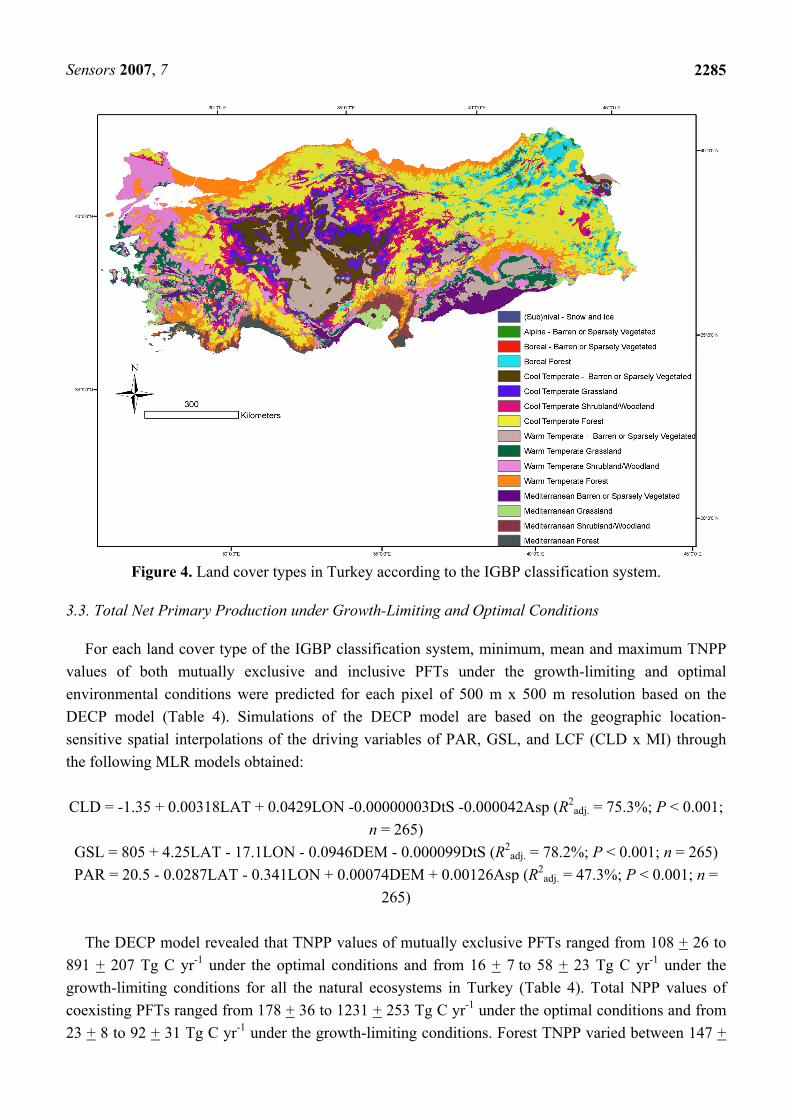
Figure 3. Spatial distribution of fractional tree cover according to the IGBP classification system. According to the IGBP land-cover classification system, the rule-based generation of potential

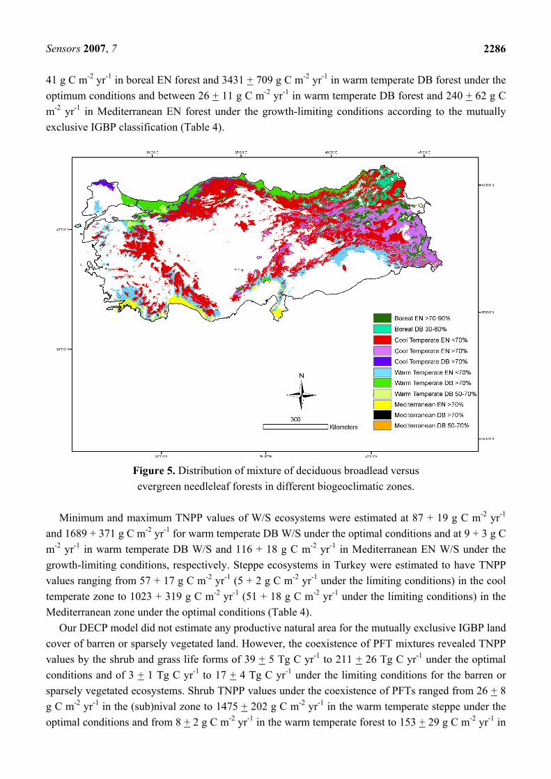
natural land cover map showed that forest (fT ≥ 60%), W/S (30% ≤ fT < 60%), grassland (steppe) (10% ≤ fT < 30%) and barren or sparsely vegetated (fT < 10%) ecosystems covered 371,097 km2 (47.5%), 150,608 km2 (19.3%), 96,533 km2 (12.4%), and 162,357 km2 (20.8%) of Turkey, respectively (Table 3). Once the digital map layers of the biogeoclimate zones and the IGBP land-cover classification were overlaid, biome-specific land cover types were determined (Figure 4). Existence, fractional cover, and spatial extent of PFT mixtures (EN versus DB forests and W/S) were determined using the gradient maps of MMTcoldest and GSP (Figure 5) (Table 3). According to the relative dominance of EN versus DB trees, 63%, 26%, and 11% of the forests appeared to be mixed (EN or DB < 70%), EN and DB forests, respectively. Pure EN forests (EN or DB ≥ 70%) range from boreal EN forests (e.g., Abies nordmanniana, and Picea orientalis) to Mediterranean EN forests (e.g., Pinus brutia, and Pinus pinea) along the MMTcoldest and GSP gradients across Turkey.

The MLR models by Paruelo and Lauenroth [35] of fS and fC3 as a function of PPT and MAT that were normalized to fT were used to estimate the coexistence and fractional cover of trees, shrubs, and C3 grass in a single pixel based on the IGBP land-cover classification (Figure 1). MLR-based spatial interpolations of PPTDJF and MAT had R2

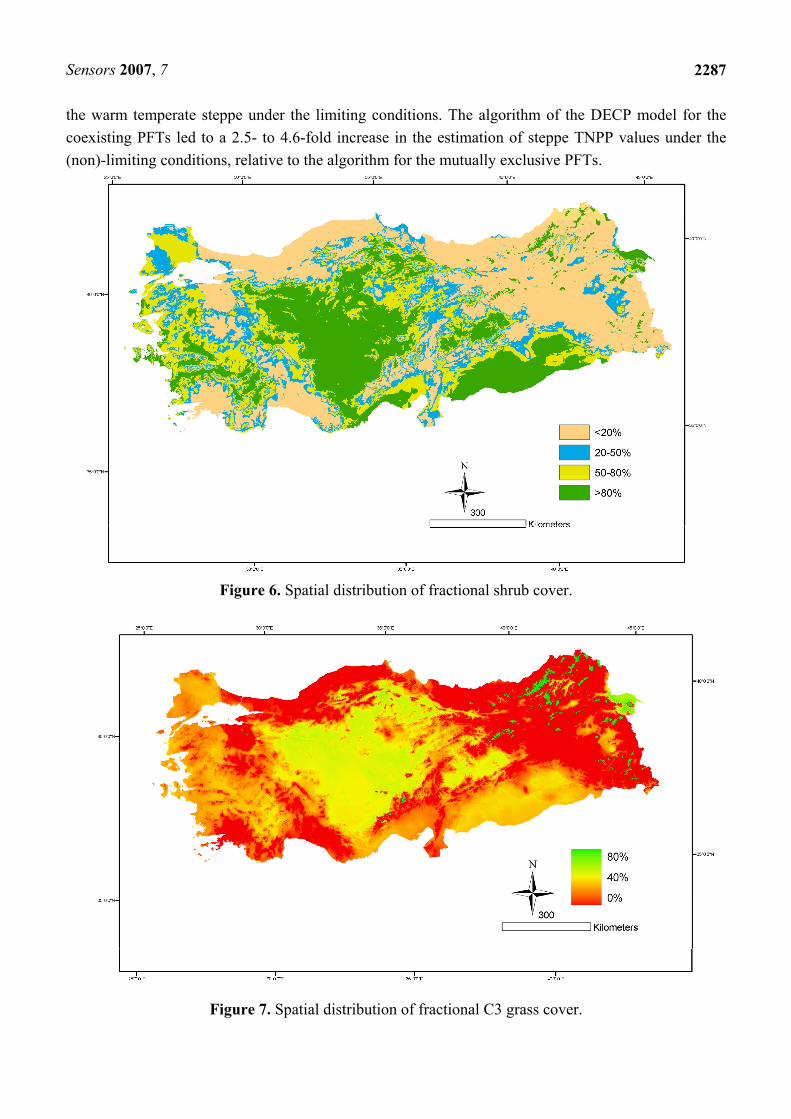
adj. values of 73.1% as a function of LAT, LON, DEM, and DtS and 90.1% as a function of LAT, LON, DEM, DtS, and aspect, respectively (P < 0.001; n = 265). Areas with fS of <20%, 20% to 50%, 50% to 80%, and >80% comprise 302,331 km2 (39%) of the eastern and northern Anatolia and southwestern Mediterranean regions; 120,030 km2 (15%) of the northwestern and central Anatolia regions; and 154,259 km2 (20%) and 203,975 km2 (26%) of the central, southeastern and western Anatolia and southeastern Mediterranean regions, respectively (Figure 6). The distribution map of C3 grass in Turkey revealed that lowland steppes are concentrated

Sensors 2007, 7

2284

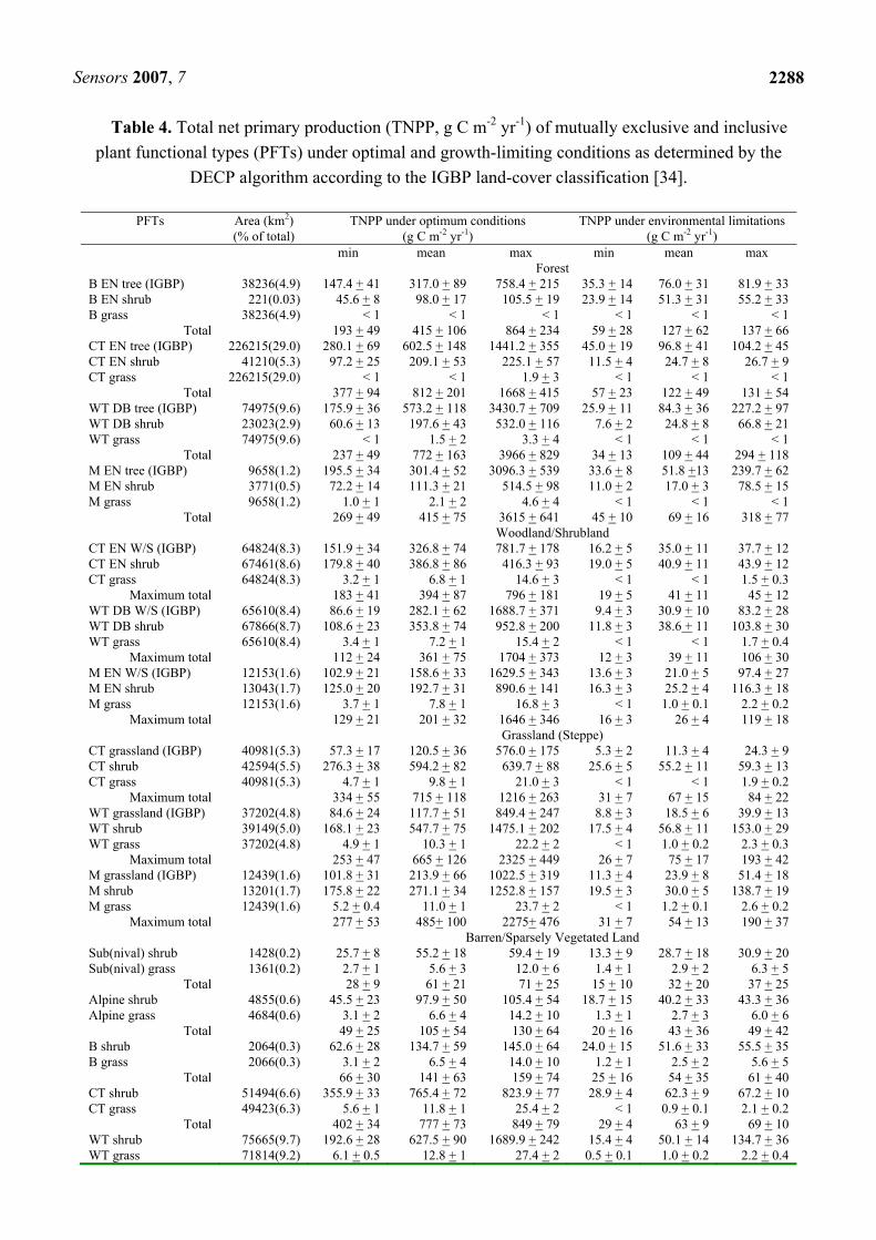
in the central and southeastern Anatolia regions, and the Iğdır plain in the eastern border of Turkey, while highland steppes mostly take place in the northeastern and eastern Anatolia regions (Figure 7).

Table 3. Biogeoclimatic distribution of plant functional type (PFT)

mixtures according to the IGBP land-cover classification.

Biogeoclimate zone

PFT EN (%)

DB (%)

Area (km2)

Percent of total land

(%) Forest (fT ≥ 60%)

Boreal EN 70-90 10-30 27900 3.6 DB, EN-DB mix 20-70 30-80 13127 1.7

Cool temperate EN-DB mix <70 >30 172184 22.1 EN ≥70 ≤30 59690 7.6 DB ≤30 ≥70 8459 1.1

Warm temperate

DB, EN-DB mix <70 >30 45591 5.8 DB ≤30 ≥70 30451 3.9

EN-DB mix 30-50 50-70 3034 0.4 Mediterranean EN ≥70 ≤30 10441 1.3

DB ≤30 ≥70 101 0.01 EN-DB mix 30-50 50-70 119 0.02

Total 371097 47.5 Shrubland/Woodland (30% ≤ fT < 60%)

Cool temperate DB ≤30 ≥70 6078 0.7 EN-DB mix 30-40 60-70 530 0.1

EN 70-80 20-30 1205 0.2 DB, EN-DB mix 20-70 30-80 60404 7.7

Warm temperate

DB ≤30 ≥70 6738 0.9 EN, EN-DB mix 30-80 20-70 62260 8.0

Mediterranean EN, EN-DB mix 30-80 20-70 13392 1.7 Total 150608 19.3

Grassland (Steppe) (10% ≤ fT < 30%) Cool temperate C3 43068 5.5 Warm temperate

C3 39837 5.1

Mediterranean C3 13629 1.7 Total 96533 12.4

Barren/Sparsely Vegetated (fT < 10%) Alpine 4997 0.6 Boreal 2218 0.3 Cool temperate 52045 6.7 Warm temperate

76653 9.8

Mediterranean 24997 3.2 Total 160910 20.6

Snow/Ice (Sub)nival 1447 0.2

Grand total 780595 100 EN: evergreen needleleaf, DB: deciduous broadleaf, fT: fractional tree cover.

Sensors 2007, 7

2285

Figure 4. Land cover types in Turkey according to the IGBP classification system.

3.3. Total Net Primary Production under Growth-Limiting and Optimal Conditions

For each land cover type of the IGBP classification system, minimum, mean and maximum TNPP values of both mutually exclusive and inclusive PFTs under the growth-limiting and optimal environmental conditions were predicted for each pixel of 500 m x 500 m resolution based on the DECP model (Table 4). Simulations of the DECP model are based on the geographic location-sensitive spatial interpolations of the driving variables of PAR, GSL, and LCF (CLD x MI) through the following MLR models obtained:

CLD = -1.35 + 0.00318LAT + 0.0429LON -0.00000003DtS -0.000042Asp (R2

adj. = 75.3%; P < 0.001; n = 265)

GSL = 805 + 4.25LAT - 17.1LON - 0.0946DEM - 0.000099DtS (R2adj. = 78.2%; P < 0.001; n = 265)

PAR = 20.5 - 0.0287LAT - 0.341LON + 0.00074DEM + 0.00126Asp (R2adj. = 47.3%; P < 0.001; n =

265)

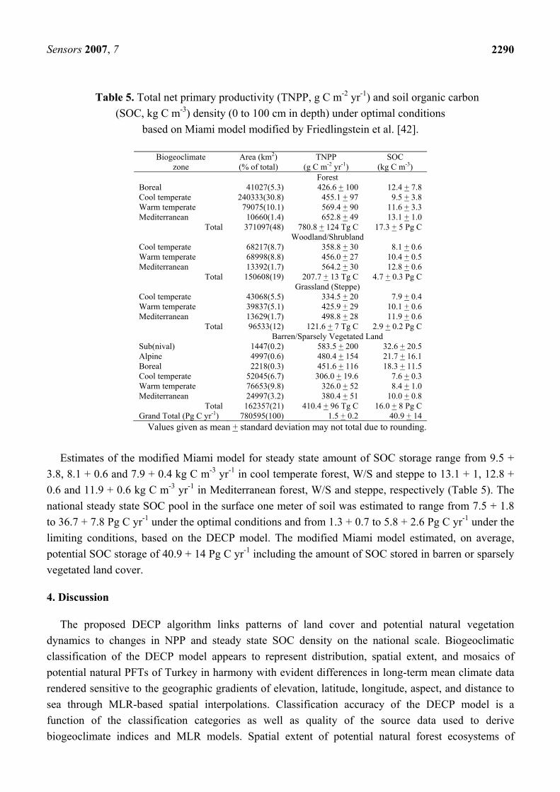
The DECP model revealed that TNPP values of mutually exclusive PFTs ranged from 108 + 26 to 891 + 207 Tg C yr-1 under the optimal conditions and from 16 + 7 to 58 + 23 Tg C yr-1 under the growth-limiting conditions for all the natural ecosystems in Turkey (Table 4). Total NPP values of coexisting PFTs ranged from 178 + 36 to 1231 + 253 Tg C yr-1 under the optimal conditions and from 23 + 8 to 92 + 31 Tg C yr-1 under the growth-limiting conditions. Forest TNPP varied between 147 +

Sensors 2007, 7

2286

41 g C m-2 yr-1 in boreal EN forest and 3431 + 709 g C m-2 yr-1 in warm temperate DB forest under the optimum conditions and between 26 + 11 g C m-2 yr-1 in warm temperate DB forest and 240 + 62 g C m-2 yr-1 in Mediterranean EN forest under the growth-limiting conditions according to the mutually exclusive IGBP classification (Table 4).

Figure 5. Distribution of mixture of deciduous broadlead versus evergreen needleleaf forests in different biogeoclimatic zones.

Minimum and maximum TNPP values of W/S ecosystems were estimated at 87 + 19 g C m-2 yr-1

and 1689 + 371 g C m-2 yr-1 for warm temperate DB W/S under the optimal conditions and at 9 + 3 g C m-2 yr-1 in warm temperate DB W/S and 116 + 18 g C m-2 yr-1 in Mediterranean EN W/S under the growth-limiting conditions, respectively. Steppe ecosystems in Turkey were estimated to have TNPP values ranging from 57 + 17 g C m-2 yr-1 (5 + 2 g C m-2 yr-1 under the limiting conditions) in the cool temperate zone to 1023 + 319 g C m-2 yr-1 (51 + 18 g C m-2 yr-1 under the limiting conditions) in the Mediterranean zone under the optimal conditions (Table 4).

Our DECP model did not estimate any productive natural area for the mutually exclusive IGBP land cover of barren or sparsely vegetated land. However, the coexistence of PFT mixtures revealed TNPP values by the shrub and grass life forms of 39 + 5 Tg C yr-1 to 211 + 26 Tg C yr-1 under the optimal conditions and of 3 + 1 Tg C yr-1 to 17 + 4 Tg C yr-1 under the limiting conditions for the barren or sparsely vegetated ecosystems. Shrub TNPP values under the coexistence of PFTs ranged from 26 + 8 g C m-2 yr-1 in the (sub)nival zone to 1475 + 202 g C m-2 yr-1 in the warm temperate steppe under the optimal conditions and from 8 + 2 g C m-2 yr-1 in the warm temperate forest to 153 + 29 g C m-2 yr-1 in

Sensors 2007, 7

2287

the warm temperate steppe under the limiting conditions. The algorithm of the DECP model for the coexisting PFTs led to a 2.5- to 4.6-fold increase in the estimation of steppe TNPP values under the (non)-limiting conditions, relative to the algorithm for the mutually exclusive PFTs.

Figure 6. Spatial distribution of fractional shrub cover.

Figure 7. Spatial distribution of fractional C3 grass cover.

Sensors 2007, 7

2288

Table 4. Total net primary production (TNPP, g C m-2 yr-1) of mutually exclusive and inclusive plant functional types (PFTs) under optimal and growth-limiting conditions as determined by the

DECP algorithm according to the IGBP land-cover classification [34].

PFTs Area (km2) (% of total)

TNPP under optimum conditions (g C m-2 yr-1)

TNPP under environmental limitations (g C m-2 yr-1)

min mean max min mean max Forest

B EN tree (IGBP) 38236(4.9) 147.4 + 41 317.0 + 89 758.4 + 215 35.3 + 14 76.0 + 31 81.9 + 33 B EN shrub 221(0.03) 45.6 + 8 98.0 + 17 105.5 + 19 23.9 + 14 51.3 + 31 55.2 + 33 B grass 38236(4.9) < 1 < 1 < 1 < 1 < 1 < 1

Total 193 + 49 415 + 106 864 + 234 59 + 28 127 + 62 137 + 66 CT EN tree (IGBP) 226215(29.0) 280.1 + 69 602.5 + 148 1441.2 + 355 45.0 + 19 96.8 + 41 104.2 + 45 CT EN shrub 41210(5.3) 97.2 + 25 209.1 + 53 225.1 + 57 11.5 + 4 24.7 + 8 26.7 + 9 CT grass 226215(29.0) < 1 < 1 1.9 + 3 < 1 < 1 < 1

Total 377 + 94 812 + 201 1668 + 415 57 + 23 122 + 49 131 + 54 WT DB tree (IGBP) 74975(9.6) 175.9 + 36 573.2 + 118 3430.7 + 709 25.9 + 11 84.3 + 36 227.2 + 97 WT DB shrub 23023(2.9) 60.6 + 13 197.6 + 43 532.0 + 116 7.6 + 2 24.8 + 8 66.8 + 21 WT grass 74975(9.6) < 1 1.5 + 2 3.3 + 4 < 1 < 1 < 1

Total 237 + 49 772 + 163 3966 + 829 34 + 13 109 + 44 294 + 118 M EN tree (IGBP) 9658(1.2) 195.5 + 34 301.4 + 52 3096.3 + 539 33.6 + 8 51.8 +13 239.7 + 62 M EN shrub 3771(0.5) 72.2 + 14 111.3 + 21 514.5 + 98 11.0 + 2 17.0 + 3 78.5 + 15 M grass 9658(1.2) 1.0 + 1 2.1 + 2 4.6 + 4 < 1 < 1 < 1

Total 269 + 49 415 + 75 3615 + 641 45 + 10 69 + 16 318 + 77 Woodland/Shrubland

CT EN W/S (IGBP) 64824(8.3) 151.9 + 34 326.8 + 74 781.7 + 178 16.2 + 5 35.0 + 11 37.7 + 12 CT EN shrub 67461(8.6) 179.8 + 40 386.8 + 86 416.3 + 93 19.0 + 5 40.9 + 11 43.9 + 12 CT grass 64824(8.3) 3.2 + 1 6.8 + 1 14.6 + 3 < 1 < 1 1.5 + 0.3

Maximum total 183 + 41 394 + 87 796 + 181 19 + 5 41 + 11 45 + 12 WT DB W/S (IGBP) 65610(8.4) 86.6 + 19 282.1 + 62 1688.7 + 371 9.4 + 3 30.9 + 10 83.2 + 28 WT DB shrub 67866(8.7) 108.6 + 23 353.8 + 74 952.8 + 200 11.8 + 3 38.6 + 11 103.8 + 30 WT grass 65610(8.4) 3.4 + 1 7.2 + 1 15.4 + 2 < 1 < 1 1.7 + 0.4

Maximum total 112 + 24 361 + 75 1704 + 373 12 + 3 39 + 11 106 + 30 M EN W/S (IGBP) 12153(1.6) 102.9 + 21 158.6 + 33 1629.5 + 343 13.6 + 3 21.0 + 5 97.4 + 27 M EN shrub 13043(1.7) 125.0 + 20 192.7 + 31 890.6 + 141 16.3 + 3 25.2 + 4 116.3 + 18 M grass 12153(1.6) 3.7 + 1 7.8 + 1 16.8 + 3 < 1 1.0 + 0.1 2.2 + 0.2

Maximum total 129 + 21 201 + 32 1646 + 346 16 + 3 26 + 4 119 + 18 Grassland (Steppe)

CT grassland (IGBP) 40981(5.3) 57.3 + 17 120.5 + 36 576.0 + 175 5.3 + 2 11.3 + 4 24.3 + 9 CT shrub 42594(5.5) 276.3 + 38 594.2 + 82 639.7 + 88 25.6 + 5 55.2 + 11 59.3 + 13 CT grass 40981(5.3) 4.7 + 1 9.8 + 1 21.0 + 3 < 1 < 1 1.9 + 0.2

Maximum total 334 + 55 715 + 118 1216 + 263 31 + 7 67 + 15 84 + 22 WT grassland (IGBP) 37202(4.8) 84.6 + 24 117.7 + 51 849.4 + 247 8.8 + 3 18.5 + 6 39.9 + 13 WT shrub 39149(5.0) 168.1 + 23 547.7 + 75 1475.1 + 202 17.5 + 4 56.8 + 11 153.0 + 29 WT grass 37202(4.8) 4.9 + 1 10.3 + 1 22.2 + 2 < 1 1.0 + 0.2 2.3 + 0.3

Maximum total 253 + 47 665 + 126 2325 + 449 26 + 7 75 + 17 193 + 42 M grassland (IGBP) 12439(1.6) 101.8 + 31 213.9 + 66 1022.5 + 319 11.3 + 4 23.9 + 8 51.4 + 18 M shrub 13201(1.7) 175.8 + 22 271.1 + 34 1252.8 + 157 19.5 + 3 30.0 + 5 138.7 + 19 M grass 12439(1.6) 5.2 + 0.4 11.0 + 1 23.7 + 2 < 1 1.2 + 0.1 2.6 + 0.2

Maximum total 277 + 53 485+ 100 2275+ 476 31 + 7 54 + 13 190 + 37 Barren/Sparsely Vegetated Land

Sub(nival) shrub 1428(0.2) 25.7 + 8 55.2 + 18 59.4 + 19 13.3 + 9 28.7 + 18 30.9 + 20 Sub(nival) grass 1361(0.2) 2.7 + 1 5.6 + 3 12.0 + 6 1.4 + 1 2.9 + 2 6.3 + 5

Total 28 + 9 61 + 21 71 + 25 15 + 10 32 + 20 37 + 25 Alpine shrub 4855(0.6) 45.5 + 23 97.9 + 50 105.4 + 54 18.7 + 15 40.2 + 33 43.3 + 36 Alpine grass 4684(0.6) 3.1 + 2 6.6 + 4 14.2 + 10 1.3 + 1 2.7 + 3 6.0 + 6

Total 49 + 25 105 + 54 130 + 64 20 + 16 43 + 36 49 + 42 B shrub 2064(0.3) 62.6 + 28 134.7 + 59 145.0 + 64 24.0 + 15 51.6 + 33 55.5 + 35 B grass 2066(0.3) 3.1 + 2 6.5 + 4 14.0 + 10 1.2 + 1 2.5 + 2 5.6 + 5

Total 66 + 30 141 + 63 159 + 74 25 + 16 54 + 35 61 + 40 CT shrub 51494(6.6) 355.9 + 33 765.4 + 72 823.9 + 77 28.9 + 4 62.3 + 9 67.2 + 10 CT grass 49423(6.3) 5.6 + 1 11.8 + 1 25.4 + 2 < 1 0.9 + 0.1 2.1 + 0.2

Total 402 + 34 777 + 73 849 + 79 29 + 4 63 + 9 69 + 10 WT shrub 75665(9.7) 192.6 + 28 627.5 + 90 1689.9 + 242 15.4 + 4 50.1 + 14 134.7 + 36 WT grass 71814(9.2) 6.1 + 0.5 12.8 + 1 27.4 + 2 0.5 + 0.1 1.0 + 0.2 2.2 + 0.4

Sensors 2007, 7

2289

Total 199 + 29 640 + 91 1717 + 244 16 + 4 51 + 14 137 + 36 M shrub 24396(3.1) 206.4 + 17 318.1 + 26 1470.3 + 121 17.4 + 3 26.9 + 5 124.1 + 21 M grass 22572(2.9) 6.5 + 0.4 13.6 + 1 29.2 + 2 < 1 1.1 + 0.2 2.5 + 0.4

Total 213 + 17 332 + 27 1500 + 123 17 + 3 28 + 5 127 + 21 Grand total (Tg C yr-1) of mutually exclusive PFTs IGBP forest 349084(44.7) 84 + 20 194 + 46 642 + 147 14 + 6 32 + 14 46 + 19 IGBP W/S 142587(18.3) 17 + 4 42 + 9 181 + 40 2 + 1 5 + 2 9 + 3 IGBP grassland 90622(11.6) 7 + 2 14 + 4 68 + 20 0.7 + 0.2 1.5 + 0.5 3 + 1

Grand total IGBP 582293(74.6) 108 + 26 250 + 60 891 + 207 16 + 7 38 + 16 58 + 23 Total shrub 471440(60.0) 86 + 13 212 + 33 437 + 67 8 + 2 20 + 5 41 + 10 Total grass 734212(94.0) 1.9 + 0.3 3.8 + 0.6 8.7 + 1.3 0.2 + 0.1 0.4 + 0.1 0.9 + 0.3 Grand total (Tg C yr-1) of mutually inclusive PFTs Total forest 349084(44.7) 90 + 22 208 + 50 666 + 153 15 + 6 33 + 14 49 + 20 Total W/S 148370(19) 22 + 5 54 + 11 184 + 40 2 + 1 6 + 2 12 + 3 Total grassland 94944(12.2) 27 + 5 65 + 11 170 + 34 3 + 1 6 + 1 13 + 3 Total BSVL 159904(20.5) 39 + 5 97 + 12 211 + 26 3 + 1 8 + 2 17 + 4

Grand total 178 + 36 424 + 84 1231 + 253 23 + 8 54 + 19 92 + 31 TNPP: total net primary productivity, B: boreal, CT: cool temperate, WT: warm temperate, M: Mediterranean, EN: evergreen needleleaf, DB: deciduous broadleaf, W/S: woodland/shrubland, BSVL: barren or sparsely vegetated land. Rows designated with and without the term “IGBP” indicate values estimated according to mutually exclusive and inclusive algorithms using the IGBP land-cover classification and MLR models by Paruelo and Lauenroth [35], respectively. Values given as mean + standard deviation may not total due to rounding.

The DECP model estimated the areal extent of productive forest ecosystems as 349,084 km2 (44.7%

of the entire country). Total spatial extent of productive steppe ecosystems was estimated as about 12% of the total land area based on the IGBP classification of mutually exclusive and inclusive PFTs with the fractional cover of 10% to 30% and as 94% of the total land area based on the MLR model [35] with the fractional cover less than 10%. Productive W/S ecosystems occupied 18% to 19% of the total land area with the fractional cover rule (30% to 60%) of the IGBP classification and 60% the total land area with the fractional cover range of 0% to 100% (Table 4).

Based on the IDW interpolation of PPT, the modified Miami model [42] was used to estimate mean TNPP values of biogeoclimatic land cover types under the optimal conditions (Table 5). Mean TNPP values estimated by the modified Miami model across Turkey ranged from 427 + 100 g C m-2 yr-1 in boreal forest to 653 + 49 g C m-2 yr-1 in Mediterranean forest; from 359 + 30 g C m-2 yr-1 in cool temperate W/S to 564 + 30 g C m-2 yr-1 in Mediterranean W/S; and from 335 + 20 g C m-2 yr-1 in cool temperate steppe to 499 + 28 g C m-2 yr-1 in Mediterranean steppe (Table 5). Sub(nival) vegetation type was estimated to have the second highest TNPP of 584 + 200 g C m-2 yr-1 after that of Mediterranean forest.

3.4. Soil Organic Carbon Density

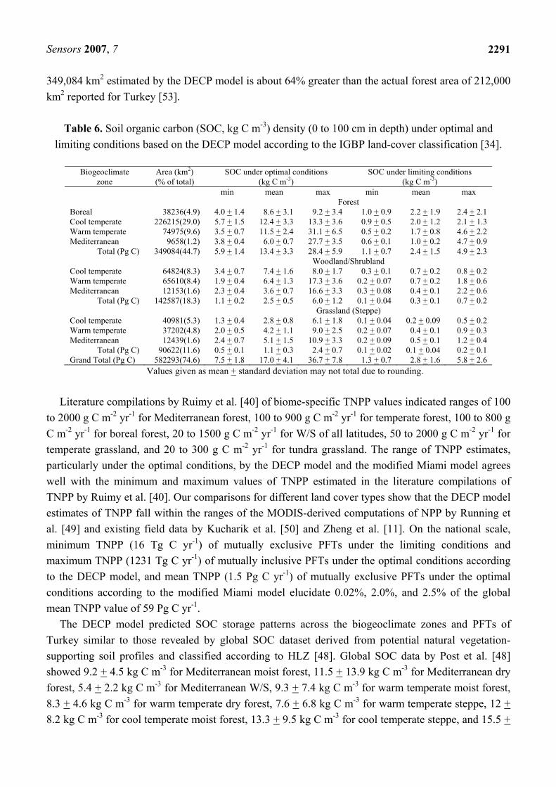
Steady state SOC density for a depth of 1 m based on the potential distribution patterns of TNPP and biogeoclimate zones, and the gradients of BT, MAT, and PPT was lowest in warm temperate forest (3.5 + 0.7 kg C m-3 yr-1) and W/S (1.9 + 0.4 kg C m-3 yr-1), and cool temperate steppe (1.3 + 0.4 kg C m-3 yr-1) and highest in warm temperate forest (31 + 7 kg C m-3 yr-1) and W/S (17 + 4 kg C m-3 yr-

1), and Mediterranean steppe (11 + 3 kg C m-3 yr-1) under the optimal conditions. Under the limiting conditions, SOC storage ranges from 0.5 + 0.2 kg C m-3 yr-1 in warm temperate forest to 4.7 + 0.9 kg C m-3 yr-1 in Mediterranean forest; from 0.2 + 0.07 kg C m-3 yr-1 in warm temperate W/S to 2.2 + 0.6 kg C m-3 yr-1 in Mediterranean W/S; and from 0.1 + 0.04 kg C m-3 yr-1 in cool temperate steppe to 1.2 + 0.4 kg C m-3 yr-1 in Mediterranean steppe (Table 6).

Sensors 2007, 7

2290

Table 5. Total net primary productivity (TNPP, g C m-2 yr-1) and soil organic carbon

(SOC, kg C m-3) density (0 to 100 cm in depth) under optimal conditions based on Miami model modified by Friedlingstein et al. [42].

Biogeoclimate

zone Area (km2) (% of total)

TNPP (g C m-2 yr-1)

SOC (kg C m-3)

Forest Boreal 41027(5.3) 426.6 + 100 12.4 + 7.8 Cool temperate 240333(30.8) 455.1 + 97 9.5 + 3.8 Warm temperate 79075(10.1) 569.4 + 90 11.6 + 3.3 Mediterranean 10660(1.4) 652.8 + 49 13.1 + 1.0

Total 371097(48) 780.8 + 124 Tg C 17.3 + 5 Pg C Woodland/Shrubland

Cool temperate 68217(8.7) 358.8 + 30 8.1 + 0.6 Warm temperate 68998(8.8) 456.0 + 27 10.4 + 0.5 Mediterranean 13392(1.7) 564.2 + 30 12.8 + 0.6

Total 150608(19) 207.7 + 13 Tg C 4.7 + 0.3 Pg C Grassland (Steppe)

Cool temperate 43068(5.5) 334.5 + 20 7.9 + 0.4 Warm temperate 39837(5.1) 425.9 + 29 10.1 + 0.6 Mediterranean 13629(1.7) 498.8 + 28 11.9 + 0.6

Total 96533(12) 121.6 + 7 Tg C 2.9 + 0.2 Pg C Barren/Sparsely Vegetated Land

Sub(nival) 1447(0.2) 583.5 + 200 32.6 + 20.5 Alpine 4997(0.6) 480.4 + 154 21.7 + 16.1 Boreal 2218(0.3) 451.6 + 116 18.3 + 11.5 Cool temperate 52045(6.7) 306.0 + 19.6 7.6 + 0.3 Warm temperate 76653(9.8) 326.0 + 52 8.4 + 1.0 Mediterranean 24997(3.2) 380.4 + 51 10.0 + 0.8

Total 162357(21) 410.4 + 96 Tg C 16.0 + 8 Pg C Grand Total (Pg C yr-1) 780595(100) 1.5 + 0.2 40.9 + 14

Values given as mean + standard deviation may not total due to rounding.

Estimates of the modified Miami model for steady state amount of SOC storage range from 9.5 +

3.8, 8.1 + 0.6 and 7.9 + 0.4 kg C m-3 yr-1 in cool temperate forest, W/S and steppe to 13.1 + 1, 12.8 + 0.6 and 11.9 + 0.6 kg C m-3 yr-1 in Mediterranean forest, W/S and steppe, respectively (Table 5). The national steady state SOC pool in the surface one meter of soil was estimated to range from 7.5 + 1.8 to 36.7 + 7.8 Pg C yr-1 under the optimal conditions and from 1.3 + 0.7 to 5.8 + 2.6 Pg C yr-1 under the limiting conditions, based on the DECP model. The modified Miami model estimated, on average, potential SOC storage of 40.9 + 14 Pg C yr-1 including the amount of SOC stored in barren or sparsely vegetated land cover.

4. Discussion

The proposed DECP algorithm links patterns of land cover and potential natural vegetation dynamics to changes in NPP and steady state SOC density on the national scale. Biogeoclimatic classification of the DECP model appears to represent distribution, spatial extent, and mosaics of potential natural PFTs of Turkey in harmony with evident differences in long-term mean climate data rendered sensitive to the geographic gradients of elevation, latitude, longitude, aspect, and distance to sea through MLR-based spatial interpolations. Classification accuracy of the DECP model is a function of the classification categories as well as quality of the source data used to derive biogeoclimate indices and MLR models. Spatial extent of potential natural forest ecosystems of

Sensors 2007, 7

2291

349,084 km2 estimated by the DECP model is about 64% greater than the actual forest area of 212,000 km2 reported for Turkey [53].

Table 6. Soil organic carbon (SOC, kg C m-3) density (0 to 100 cm in depth) under optimal and

limiting conditions based on the DECP model according to the IGBP land-cover classification [34].

Biogeoclimate zone

Area (km2) (% of total)

SOC under optimal conditions (kg C m-3)

SOC under limiting conditions (kg C m-3)

min mean max min mean max Forest

Boreal 38236(4.9) 4.0 + 1.4 8.6 + 3.1 9.2 + 3.4 1.0 + 0.9 2.2 + 1.9 2.4 + 2.1 Cool temperate 226215(29.0) 5.7 + 1.5 12.4 + 3.3 13.3 + 3.6 0.9 + 0.5 2.0 + 1.2 2.1 + 1.3 Warm temperate 74975(9.6) 3.5 + 0.7 11.5 + 2.4 31.1 + 6.5 0.5 + 0.2 1.7 + 0.8 4.6 + 2.2 Mediterranean 9658(1.2) 3.8 + 0.4 6.0 + 0.7 27.7 + 3.5 0.6 + 0.1 1.0 + 0.2 4.7 + 0.9

Total (Pg C) 349084(44.7) 5.9 + 1.4 13.4 + 3.3 28.4 + 5.9 1.1 + 0.7 2.4 + 1.5 4.9 + 2.3 Woodland/Shrubland

Cool temperate 64824(8.3) 3.4 + 0.7 7.4 + 1.6 8.0 + 1.7 0.3 + 0.1 0.7 + 0.2 0.8 + 0.2 Warm temperate 65610(8.4) 1.9 + 0.4 6.4 + 1.3 17.3 + 3.6 0.2 + 0.07 0.7 + 0.2 1.8 + 0.6 Mediterranean 12153(1.6) 2.3 + 0.4 3.6 + 0.7 16.6 + 3.3 0.3 + 0.08 0.4 + 0.1 2.2 + 0.6

Total (Pg C) 142587(18.3) 1.1 + 0.2 2.5 + 0.5 6.0 + 1.2 0.1 + 0.04 0.3 + 0.1 0.7 + 0.2 Grassland (Steppe)

Cool temperate 40981(5.3) 1.3 + 0.4 2.8 + 0.8 6.1 + 1.8 0.1 + 0.04 0.2 + 0.09 0.5 + 0.2 Warm temperate 37202(4.8) 2.0 + 0.5 4.2 + 1.1 9.0 + 2.5 0.2 + 0.07 0.4 + 0.1 0.9 + 0.3 Mediterranean 12439(1.6) 2.4 + 0.7 5.1 + 1.5 10.9 + 3.3 0.2 + 0.09 0.5 + 0.1 1.2 + 0.4

Total (Pg C) 90622(11.6) 0.5 + 0.1 1.1 + 0.3 2.4 + 0.7 0.1 + 0.02 0.1 + 0.04 0.2 + 0.1 Grand Total (Pg C) 582293(74.6) 7.5 + 1.8 17.0 + 4.1 36.7 + 7.8 1.3 + 0.7 2.8 + 1.6 5.8 + 2.6

Values given as mean + standard deviation may not total due to rounding.

Literature compilations by Ruimy et al. [40] of biome-specific TNPP values indicated ranges of 100

to 2000 g C m-2 yr-1 for Mediterranean forest, 100 to 900 g C m-2 yr-1 for temperate forest, 100 to 800 g C m-2 yr-1 for boreal forest, 20 to 1500 g C m-2 yr-1 for W/S of all latitudes, 50 to 2000 g C m-2 yr-1 for temperate grassland, and 20 to 300 g C m-2 yr-1 for tundra grassland. The range of TNPP estimates, particularly under the optimal conditions, by the DECP model and the modified Miami model agrees well with the minimum and maximum values of TNPP estimated in the literature compilations of TNPP by Ruimy et al. [40]. Our comparisons for different land cover types show that the DECP model estimates of TNPP fall within the ranges of the MODIS-derived computations of NPP by Running et al. [49] and existing field data by Kucharik et al. [50] and Zheng et al. [11]. On the national scale, minimum TNPP (16 Tg C yr-1) of mutually exclusive PFTs under the limiting conditions and maximum TNPP (1231 Tg C yr-1) of mutually inclusive PFTs under the optimal conditions according to the DECP model, and mean TNPP (1.5 Pg C yr-1) of mutually exclusive PFTs under the optimal conditions according to the modified Miami model elucidate 0.02%, 2.0%, and 2.5% of the global mean TNPP value of 59 Pg C yr-1.

The DECP model predicted SOC storage patterns across the biogeoclimate zones and PFTs of Turkey similar to those revealed by global SOC dataset derived from potential natural vegetation-supporting soil profiles and classified according to HLZ [48]. Global SOC data by Post et al. [48] showed 9.2 + 4.5 kg C m-3 for Mediterranean moist forest, 11.5 + 13.9 kg C m-3 for Mediterranean dry forest, 5.4 + 2.2 kg C m-3 for Mediterranean W/S, 9.3 + 7.4 kg C m-3 for warm temperate moist forest, 8.3 + 4.6 kg C m-3 for warm temperate dry forest, 7.6 + 6.8 kg C m-3 for warm temperate steppe, 12 + 8.2 kg C m-3 for cool temperate moist forest, 13.3 + 9.5 kg C m-3 for cool temperate steppe, and 15.5 +

Sensors 2007, 7

2292

30 kg C m-3 for boreal moist forest. The estimates of SOC values under the optimal conditions by the DECP and modified Miami models are well within one standard deviation of the global SOC dataset by Post et al. [48]. Our national range of estimates for SOC storage of 1.3 Pg C to 36.7 Pg C by the DECP model and 40.9 Pg C by the modified Miami model accounts for 0.1%, 2.8%, and 3.2% of the global SOC value (1272.4 Pg C) according to Post et al. [48], respectively.

According to DECP, mean SOC carbon density appeared to decrease for forest and W/S ecosystems and increase for steppe ecosystems in transition from cool temperate to Mediterranean zones. This pattern for forest and W/S reveals that SOC storage decreases in response to an increase in BT and PER (the ratio of PETHLZ to PPT), and a decrease in elevation and GSP. When PER (1.1 + 0.35) approached unity in the cool temperate zone, SOC pool under the cool temperate forest peaked at 12.4 + 3.3 kg C m-3 which shows a close agreement with mean SOC pool value of 10 kg C m-3 at PER of 1 derived from the global soil dataset [48]. The reverse pattern for steppe ecosystems appears to be due to the increase in TNPP values estimated in transition from cool temperate to Mediterranean zones. On the other hand, the modified Miami model estimated increases in TNPP and SOC for forest, W/S and steppe ecosystems in transition from cool temperate to Mediterranean zones and failed to capture detailed patterns among biogeoclimate variables, SOC storage and TNPP revealed by the DECP algorithm.

Values of vegetation-specific parameters used in the DECP model approximately correspond to those of the biogeochemical models TEM [23], CASA [51] and SILVAN [52]. As with all regression models, MLR models should be used cautiously to estimate response variables at large spatial scales beyond the region from which they are derived. The proposed DECP model does not account for certain areas of a grid cell that may be unsuitable for establishment of natural vegetation (including rivers, lakes, roads, and rock and stony outcrops), and for changes caused by human disturbances (deforestation, urban sprawl, and land-use changes). The model must be further validated by other means available such as satellite images before its use in predicting spatio-temporal responses of biogeoclimate zones, PFTs, TNPP, and SOC to the projected scenarios of global climate change [56]. According to available field and remotely sensed data, the DECP model based on the 37-year mean climatic data was able to generate realistic distributions of potential natural land cover and estimates of TNPP and steady state SOC in Turkey under the limiting and non-limiting conditions in mutually exclusive and inclusive ways of PFTs. The difference between the steady state estimates of net C stocks for potential natural ecosystems under the non-limiting and limiting conditions may reveal the magnitude of historic national C loss as well as the national potential for C sequestration if 50% recovery of C loss is assumed over the next 50-100 years as a reasonable upper limit in constant climate.

This research provides the first extensive quantification of potential conditions for NPP and SOC in Turkey. Coupling this information with current land-use/land-cover and related NPP would lead to important implications about C loss due to human-induced disturbances across Turkey since most of the C loss is most likely to result from alteration of land-use/land-cover, and land management practices. Our model potentially estimated ca. 45% of the land area of Turkey to be productive forest ecosystems, while only ca. 25% of the country is currently forested, with more than half being unproductive. This reveals the significant potential for Turkey’s forests to sequester C as well as the importance of sustainable land management practices to achieve C-sequestration potential given rapid

Sensors 2007, 7

2293

rates of population growth and conversions of forests and grasslands into urban-industrial and cropland areas.

Acknowledgements

We gratefully acknowledge the research project grant (KARIYER-TOVAG-104O550) from the Scientific and Technological Research Council (TUBITAK) of Turkey and the Research Project Administration Units of Abant Izzet Baysal University, Cukurova University, and Akdeniz University.

References

1. Behrenfeld, M.J.; Randerson, J.T.; McClain, C.R.; Feldman, G.C.; Los, S.O.; Tucker, C.J.; Falkowski, P.G.; Field, C.B.; Frouin, R.; Esaias, W.E.; Kolber, D.D.; Pollack, N.H. Biospheric primary production during an ENSO transition. Science 2001, 291, 2594–2597.

2. Hicke, J.A.; Asner, G.P.; Randerson, J.T.; Tucker, C.J.; Los, S.; Birdsey, R.; Jenkins, J.C.; Field, C. Trends in North American net primary productivity derived from satellite observations, 1982–1998. Global Biogeochemical Cycles 2002, 16, 1018 (doi:10.1029/2001GB001550).

3. Nemani, R.R.; Keeling, C.D.; Hashimoto, H.; Jolly, W.M.; Piper, S.C.; Tucker, C.J.;Myneni, R.B.; Running, S.W. Climate-driven increases in global terrestrial net primary production from 1982 to 1999. Science 2003, 300, 1560–1563.

4. Potter, C.; Klooster, S.; Myneni, R.; Genovese, V.; Tan, P.; Kumar, V. Continental scale comparisons of terrestrial carbon sinks estimated from satellite data and ecosystem modeling 1982-98. Global Planetary Change 2003, 39, 201–213.

5. Hashimoto, H.; Nemani, R.R.; White, M.A.; Jolly, W.M.; Piper, S.C.; Keeling, C.D.; Myneni, R.B.; Running, S.W. El Niño–Southern Oscillation–induced variability in terrestrial carbon cycling. Journal of Geophysical Research 2004, 109, D23110 (doi:10.1029/2004JD004959).

6. Field, C.B.; Behrenfeld, M.J.; Randerson, J.T.; Falkowski, P.G. Primary production of the biosphere: integrating terrestrial and oceanic components. Science 1998, 281, 237–240.

7. Adams, B.; White, A.; Lenton, T.M. An analysis of some diverse approaches to modelling terrestrial net primary productivity. Ecological Modelling 2004, 177, 353–391.

8. Evrendilek, F.; Wali, M.K. Changing global climate: historical carbon and nitrogen budgets and projected responses of Ohio’s cropland ecosystems. Ecosystems 2004, 7, 381–392.

9. Wali, M.K.; Evrendilek, F.; West, T.; Watts, S.; Pant, D.; Gibbs, H.; McClead, B. Assessing terrestrial ecosystem sustainability: usefulness of regional carbon and nitrogen models. Nature & Resources 1999, 35, 20–33.

10. Pan, Y.; Li, X.; Gong, P.; He, C.; Shi, P.; Pu, R. An integrative classification of vegetation in China based on NOAA AVHRR and vegetation–climate indices of the Holdridge life zone. International Journal of Remote Sensing 2003, 24, 1009–1027.

11. Zheng, D.; Prince, S.; Wright, R. Terrestrial net primary production estimates for 0.5° grid cells from field observations—a contribution to global biogeochemical modeling. Global Change Biology 2003, 9, 46–64.

12. Wilson, M.F.; Henderson-Sellers, A. A global archive of land cover and soils data for use in general circulation climate models. Journal of Climatology 1985, 5, 119–143.

Sensors 2007, 7

2294

13. DeFries, R.S.; Townshend, J.R.G. NDVI-derived land cover classification at a global scale. International Journal of Remote Sensing 1994, 15, 3567–3586.

14. Köppen W. Das geographische system der klimate. In Handbuch der Klimatologie; Koppen, W.; Geiger, R., Eds.; Borntrager: Berlin, 1936; pp 1–40.

15. Holdridge, L.R. Determination of world plant formations from simple climate data. Science 1947, 105, 367–368.

16. Box, E.O. Factors determining distributions of tree species and plant functional types. Vegetation 1995, 121, 101–116.

17. Krajina, V.J. Biogeoclimatic zones and biogeocoenoses of British Columbia. Ecology of Western North America 1965, 1, 1–17.

18. Box, E.O. Predicting physiognomic vegetation types with climate variables. Vegetatio 1981, 45, 127–139.

19. Bailey, R.G. Delineation of ecosystem regions. Environmental Management 1983, 7, 365–373. 20. Ollinger, S.V.; Aber, J.D.; Federer, C.A. Estimating regional forest productivity and water yield

using an ecosystem model linked to a GIS. Landscape Ecology 1998, 13, 323–334. 21. Running, S.W.; Coughlan, J.C. A general model of forest ecosystem processes for regional

applications, I. hydrologic balance, canopy gas exchange and primary production processes. Ecological Modelling 1988, 42, 125–154.

22. Burke, I.C.; Schimel, D.S.; Yonker, C.M.; Parton, W.J.; Joyce, L.A.; Lauenroth, W.K. Regional modeling of grassland biogeochemistry using GIS. Landscape Ecology 1990, 4, 45–54.

23. Raich, J.W.; Rastetter, E.B.; Melillo, J.M.; Kicklighter, D.W.; Steudler, P.A.; Peterson, B.J.; Grace, A.L.; Moore B. III; Vorosmarty, C.J. Potential net primary productivity in South-America-application of a global-model. Ecological Applications 1991, 1, 399–429.

24. Daly, C.; Neilson, R.P.; Phillips, D.L. A statistical-topographical model for mapping climatological precipitation over mountainous terrain. Journal of Applied Meteorology 1994, 33, 140–158.

25. Aber, J.D.; Ollinger, S.V.; Federer, C.A.; Reich, P.B.; Goulden, M.L.; Kicklighter, D.W.; Melillo, J.M.; Lathrop, J.R.G. Predicting the effects of climate change on water yield and forest production in the northeastern US. Climate Research 1995, 5, 207–222.

26. Kicklighter, D.W.; Bondeau, A.; Schloss, A.L.; Kaduk, J.; McGuire, A.D.; the Participants of the Potsdam NPP Model Intercomparison. Comparing global models of terrestrial net primary productivity (NPP): Global pattern and differentiation by major biomes. Global Change Biology 1999, 5, 16–24.

27. Evrendilek, F.; Wali, M.K. Modelling long-term C dynamics in croplands in the context of climate change: a case study from Ohio. Environmental Modelling & Software 2001, 16, 361–375.

28. Stanley, D.J.; Wezel, F.-C. Geological evolution of the Mediterranean Basin. Springer-Verlag: New York, 1985.

29. GDRS (General Directorate of Rural Services). Digital soil map. Soil and Water Resources National Information Centre: Ankara, 2006.

30. Oakes, H. The soils of Turkey. Ministry of Agriculture, Soil Conservation and Farm Irrigation Division Ministry of Agriculture Publishers: Ankara, 1958.

Sensors 2007, 7

2295

31. Soil Survey Staff. Soil classification: a comprehensive system, 7th Approximation. U.S. Governmental Print Office: Washington, D.C., 1960.

32. TSMS (Turkish State Meteorological Service). Monthly climate data between 1968 and 2004. Turkish State Meteorological Service: Ankara, 2005.

33. Woodward, F.I. Climate and plant distribution. Cambridge University Press: New York, 1987. 34. Loveland, T.R.; Reed, B.C.; Brown, J.F.; Ohlen, D.O.; Zhu, Z.; Yang, L.; Merchant, J.W.

Development of a global land cover characteristics database and IGBP DISCover from 1-km AVHRR data. International Journal of Remote Sensing 2000, 6, 1303–1330.

35. Paruelo, J.M.; Lauenroth, W.K. Climatic controls of the distribution of plant functional types in grasslands and shrublands of North America. Ecological Applications 1996, 6, 1212–1224.

36. ESRI Inc. ArcGIS 8.2. ESRI Inc.: Redlands, 2002. 37. Monteith, J.L. Solar radiation and productivity in tropical ecosystems. Journal of Applied Ecology

1972, 9, 747–766. 38. Monteith, J.L. Climate and the efficiency of crop production in Britain. Philosophical

Transactions of the Royal Society B-Biological Sciences 1977, 281, 277–294. 39. Kumar, M.; Monteith, J.L. Remote sensing of crop growth. In Plants and the Daylight Spectrum;

Smith, H., Ed.; Academic Press: London, 1981, pp. 133–144. 40. Ruimy, A.; Saugier, B.; Dedieu, G. Methodology for the estimation of terrestrial primary

production from remotely sensed data. Journal of Geophysical Research 1994, 99, 5263–5283. 41. McCree, K.J. Test of current definitions of photosynthetically active radiation against leaf

photosynthesis data. Agricultural Meteorology 1972, 10, 443–453. 42. Friedlingstein, P.; Delire, C.; Muller, J.F.; Gerard, J.C. The climate induced variation of the

continental biosphere: a model simulation of the Last Glacial Maximum. Geophysical Research Letters 1992, 19, 897–900.

43. Leith, H. Modeling the primary productivity of the world. In Primary productivity of the Biosphere; Leith, H.; Whittaker, R.H., Eds.; Springer-Verlag: New York, 1975, pp. 237–262.

44. Dai, A.; Fung, I.Y. Can climate variability contribute to the `missing´ CO2 sink? Global Biogeochemical Cycles 1993, 7, 599–609.

45. Jenny, H. Factors of soil formation. McGraw-Hill: New York, 1941. 46. Zinke, P.J.; Stangenberger, A.G.; Post, W.P.; Emanual, W.R.; Olson, J.S. Worldwide organic soil

carbon and nitrogen data. ORNL/NDP–018, Oak Ridge National Laboratory, Oak Ridge, Tennessee, 1986.

47. Yang, X.; Wang, M.; Huang, Y.; Wang, Y. A one-compartment model to study soil carbon decomposition rate at equilibrium situation. Ecological Modelling 2002, 151, 63–73.

48. Post, W.M.; Pastor, J.; Zinke, P.J.; Stangenberger, A.G. Global patterns of soil nitrogen storage. Nature 1985, 317, 613–616.

49. Running, S.W.; Ramakrishna, R.N.; Heinsch, F.A.; Zhao, M.; Reeves, M.; Hashimotoa, H. Continuous satellite-derived measure of global terrestrial primary production. BioScience 2004, 54, 547–560.

50. Kucharik, C.J.; Foley, J.A.; Delire, C.; Fisher, V.A.; Coe, M.T.; Lenters, J.D.; Young-Molling, C.; Ramankutty, N.; Norman, J.M.; Gower, S.T. Testing the performance of a dynamic global

Sensors 2007, 7

2296

ecosystem model: water balance, carbon balance, and vegetation structure. Global Biogeochemical Cycles 2000, 14, 795–825.

51. Potter, C.S.; Randerson, J.T.; Field, C.B.; Matson, P.A.; Vitousek, P.M.; Mooney, H.A.; Klooster, S.A. Terrestrial ecosystem production: A process model based on global satellite and surface data. Global Biogeochemical Cycles 1993, 7, 811–841.

52. Kaduk, J.; Heimann, M. Assessing the climate sensitivity of the global terrestrial carbon cycle model SILVAN. Physics and Chemistry of the Earth 1996, 21, 529–535.

53. Kaya, Z.; Raynal, D.J. Biodiversity and conservation of Turkish forests. Biological Conservation 2001, 97, 131–141.

54. Yue, T.X.; Fan, Z.M.; Liu, J.Y. Changes of major terrestrial ecosystems in China since 1960. Global Planetary Change 2005, 48, 287–302.

55. Zheng, Y.; Xie, Z.; Jiang, L.; Shimizu, H.; Drake, S. Changes in Holdridge Life Zone diversity in the Xinjiang Uygur Autonomous Region (XUAR) of China over the past 40 years. Journal of Arid Environments 2006, 66, 113–126.

56. Berberoglu, S.; Evrendilek, F.; Ozkan, C.; Donmez, C. Modeling forest productivity using Envisat MERIS data. Sensors 2007, 7 (10), 2115–2127.

© 2007 by MDPI (http://www.mdpi.org). Reproduction is permitted for noncommercial purposes.