Modeling purchases of new cars: an analysis of the 2014French market

Anna Fernández Antolín ∗ Matthieu de Lapparent ∗ Michel Bierlaire ∗

Report TRANSP-OR 161130Transport and Mobility Laboratory

École Polytechnique Fédérale de Lausannetransp-or.epfl.ch

∗Transp-OR, Ecole Polytechnique Fédérale de Lausanne, CH-1015 Lausanne, Switzerland,{anna.fernandezantolin,matthieu.delapparent,michel.bierlaire}@epfl.ch

i

Abstract

This paper analyses and compares different policy scenarios as well as discusses price elastic-ities and willingness to pay and to accept using revealed preference data from the French new-carmarket in 2014 by means of a cross-nested logit (CNL) model. We focus particularly on electricand hybrid vehicles. We use interactions between the cost (both fixed and running costs) and thehousehold income in order to analyze the sensitivity towards different policy scenarios per incomelevel.

Results show that the willingness to pay and to accept obtained in our study are consistentwith the real market conditions. We also find that the most effective scenario in order to increasethe market shares of new sold electric vehicles is that of a major technological advance such as adecrease in price due to cheaper manufacturing costs and an increase in driving range, rather thana policy-based scenario. Also, the market segment that has more potential to increase the marketshares of electric vehicle purchase is the middle-income level.

In the paper, we discuss how to overcome the difficulties of working with revealed preferencedata, and propose a new method to impute the attributes of the unchosen alternatives, based on theempirical distributions observed in the data.

Keywords: car-type choice, policy analysis, revealed preference data, cross-nested logit

ii

1 IntroductionThe automobile sector is of interest for both the public and the private sectors. Governments and otherpublic actors need to understand the car market in order to have valid forecasts of energy consumption,emission levels and even tax revenue. By means of these forecasts they can also derive optimal policymeasures to, for instance, promote the use of electric vehicles to reduce emissions.

It is also interesting for private companies. The interest from automobile firms is obvious, but thecar market is linked to many other sectors such as those providing the raw materials (steel, chemicals,textiles) and those working with automobiles such as repair and mobility services. Moreover, accord-ing to the European Commission, “the EU is among the world’s biggest producers of motor vehiclesand the sector represents the largest private investor in research and development (R&D)” 1

In order to satisfy the needs of these public and private actors it is important to model car owner-ship, which has many dimensions. Car ownership models can be classified based on several criteriaaccording to de Jong et al. (2004) such as: i) the inclusion of supply and demand, ii) the aggregationlevel, iii) the time representation (dynamic or static), iv) the time horizon (long-term or short-termforecasts), v) the inclusion of car-use and other socioeconomic characteristics, and vi) the type ofmarket (private or business cars) among others. In this paper we focus on the demand side of privatecars, in a disaggregate and static framework where we include socioeconomic characteristics of thecar buyers. The objective is to have long-term forecasts. This is known as static disaggregate car-typechoice models.

Our goal is to use revealed preference data to estimate these type of models. This allows to havemore realistic demand indicators compared to the ones obtained with stated preference data, such aspredicted market shares under several scenarios, willingness to pay and to accept several car attributesand price elasticities. We are particularly interested in the demand for hybrid and electric vehicles.Using RP is more challenging. The main difficulties are to define the choice set and to define theattributes of the unchosen alternatives. The main contribution of the paper is the way how we definethe attributes of the unchosen alternatives. We use the empirical distribution of the attributes and drawfrom them.

The remaining of the paper is structured as follows. Section 2 contains a brief literature review,which is followed by the description of the data used in the paper, and how it is aggregated into dif-ferent choice alternatives in Section 3. In Section 4 we discuss the adopted methodological approach,the results of which are discussed in Section 5. The application of the model is discussed in Section 6.We finalize the paper with some concluding remarks and future research directions in Section 7.

2 Literature ReviewAs mentioned in Section 1, we focus on static disaggregate car-type choice models. The first studydealing with this type of models was performed by Lave & Train (1979). For a complete review of theliterature on car ownership the reader is refered to de Jong et al. (2004) and more recently to Anowaret al. (2014).

1http://ec.europa.eu/growth/sectors/automotive

1

Although it is clear that a choice of a private car is a discrete choice, there does not seem to beconsensus in the literature about the definition of the choice set. The two main approaches are definedbelow. The first approach considers that a car is characterized by its make, model, engine and vintage(Birkeland & Jordal-Jorgensen, 2001). Then, for a given year, there may be over 1,000 alternatives. Inthis case, sampling of alternatives is usually required for the estimation of the model, although recentdevelopments in model estimation (Mai et al. , 2015) allow to estimate large scale MEV models.

The second approach prefers an aggregate representation. For example Page et al. (2000) char-acterize a car by its engine size and fuel type. They have nine alternatives for petrol and seven fordiesel. It greatly simplifies the specification and estimation of the model. A similar aggregation ofalternatives is used by Hess et al. (2012). This approach is also justifiable from a behavioral point ofview, arguing that decision-makers do not explicitly consider large choice sets.

The most popular model in this context is logit (Wu et al. , 1999; Choo & Mokhtarian, 2004).However, the Independence from Irrelevant Alternatives (IIA) property of logit, may lead to counter-intuitive results when alternatives share unobserved attributes. It is likely to happen in car-type choiceno matter which of the previous two approaches is chosen. Other models have been considered, suchas mixtures of logit models, (Brownstone & Train, 1998; McFadden et al. , 2000; Potoglou, 2008),nested logit models (Berkovec & Rust, 1985; McCarthy & Tay, 1998; Mohammadian & Miller, 2002,2003; Cao et al. , 2006) and cross nested logit models (Hess et al. , 2012).

The interest in electric and hybrid vehicles has risen in the past years, through the analysis ofstated preferences data (Glerum et al. , 2014; Hackbarth & Madlener, 2016; Beck et al. , 2013, 2016;Daziano, 2013; Hackbarth & Madlener, 2013; Daziano & Achtnicht, 2014; Brownstone & Train,1998; Train, 1980). Massiani (2014) describes some of the most important limitations of the statedpreference surveys being used currently in the literature, and questions the policy recommendationsthat can be obtained from them. Studies carried out with revealed preference data are generallyquite old, and do not focus on electric and alternative fuel vehicles, mainly because of limitation ofthese vehicles in revealed preference data. Some examples include Berry et al. (1995, 1998); Train(1986); Berkovec (1985); Train & Winston (2007). In these studies aggregation of alternatives isused. Berkovec & Rust (1985) instead use sampling of alternatives, where 14 out of 785 alternativesare sampled for estimation. The main difficulty when using revealed preference data is to imputethe attributes of the unchosen alternatives, in particular if there is an aggregation of alternatives.The studies cited above deal with it by imputing mean values of the attributes for each unchosenalternative.

We fill the gap in the literature by proposing an alternative way of imputing the attributes of theunchosen alternatives, based on multiple imputation using the empirical distributions of the attributesfor each alternative. To the best of our knowledge, it is also the first study of car-type choice to focuson electric and hybrid vehicles in the context of the whole market using revealed preference data.Due to the lack of variability in the autonomy (the range) of electric vehicles that are currently in themarket, we need to take the value of the willingness to pay for range from the literature. By doing thiswe are able forecast the impact of an increase of the range on the market shares of electric vehicles.We validate our model with demand indicators such as market shares, elasticities and willingness topay and to accept.

2

3 Data and data aggregationWe use a dataset reporting sales of new cars in France in 2014. Each observation corresponds tothe purchase of a new car. The dataset reports over 40,000 purchases. However, after selectingthe variables that we use in the model and removing the missing values for any of them, 18,804observations are used for this study. It is left for future work to recover some of these missing values.

In our approach we decide to consider a car-type as a combination between a market segment anda fuel type. The market segments are full, luxury, medium, multipurpose vehicles (MPV), off-road andsmall2. The fuel types considered are diesel, petrol, electric and hybrid. Table 1 gives some examplesof cars belonging to each market segment.

Market segment Car

FullFord TaurusToyota AvalonHyundai Grandeur

LuxuryMercedes-Benz S-ClassAudi A8BMW 7 Series

MediumOpel AstraHonda CivicAudi A3

Multipurpose vehicleRenault EspaceVolkswagen SharanMercedes-Benz Vito

Off-roadLand Rover FreelanderChevrolet CaptivaBMW X5

SmallOpel CorsaFord FiestaToyota Yaris

Table 1: Examples of cars that belong to each market segment.

Out of the 18,804 observations, only 657 report the purchase of a hybrid vehicle. Moreover, theyare always combined with either diesel or petrol. Consequently, we consider hybrid as a marketsegment rather than as a fuel type. Therefore, we have a total of 15 alternatives summarized inTable 2, together with the number of observations corresponding to each alternative after removingany missing values. Note that we should have 21 alternatives (3 fuel types multiplied by 7 market

2These segments are derived from the European Commission’s segmentation

3

segments). The six missing alternatives are the combinations of electric vehicles with any marketsegment except small. This is because these alternatives do not exist in the French market. The onlyexception is electric luxury vehicles, that do exist (e.g: Tesla), but represent a negligible part of thecar market. For this reason, we decide to remove this alternative (electric luxury) from the analysis.

Alternative Market segment Fuel type Nbr. of obs.

1 Full Diesel 3232 Luxury Diesel 1783 Medium Diesel 2,2264 MPV Diesel 1,3755 Off-road Diesel 2,0446 Small Diesel 5,5387 Hybrid Diesel 1618 Full Petrol 689 Luxury Petrol 5410 Medium Petrol 66311 MPV Petrol 31012 Off-road Petrol 26513 Small Petrol 5,03714 Hybrid Petrol 49615 Small Electric 66

Total 18,804

Table 2: List of alternatives in the choice set and number of observations (after removing missing values).

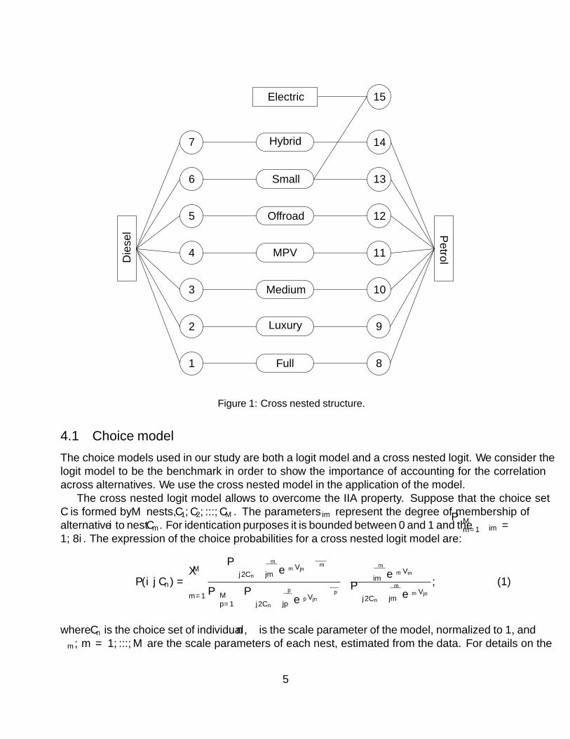
From this definition of alternatives, it is obvious that alternatives that share either fuel type ormarket segment share unobserved attributes. Figure 1 proposes a correlation structure derived fromthe multi-dimensional nature of the choice set presented in Table 2. This correlation structure is usedin the cross nested logit model presented in Section 4.

We assume that our dataset is representative of the population of new car buyers from an exoge-nous point of view (i.e: from a socioeconomic point of view). It is important to note that it might notbe representative of the whole French population, but this is not an issue. For the representativeness ofthe choices, we are able to replicate the real market shares by applying the correction of the alternativespecific constants as described by Train (2009).

4 Methodological approach and model specificationThis section contains the methodological approach used to estimate the choice model. We define thechoice model used in Section 4.1 followed by the model specification, the nesting structure and thedefinition of the variables used in Section 4.2. We finalize by describing how we import the parameterassociated with range from the literature in Section 4.3.

4

1

2

3

4

5

6

7

Full

Luxury

Medium

MPV

Offroad

Small

Hybrid

Electric

8

9

10

11

12

13

14

15

Die

sel Petrol

Figure 1: Cross nested structure.

4.1 Choice modelThe choice models used in our study are both a logit model and a cross nested logit. We consider thelogit model to be the benchmark in order to show the importance of accounting for the correlationacross alternatives. We use the cross nested model in the application of the model.

The cross nested logit model allows to overcome the IIA property. Suppose that the choice setC is formed by M nests, C1, C2, ..., CM. The parameters αim represent the degree of membership ofalternative i to nest Cm. For identification purposes it is bounded between 0 and 1 and the

∑Mm=1 αim =

1, ∀i. The expression of the choice probabilities for a cross nested logit model are:

P(i | Cn) =M∑m=1

(∑j∈Cn α

µmµ

jm eµmVjn) µµm

∑Mp=1

(∑j∈Cn α

µpµ

jp eµpVjn) µµp

· αµmµ

im eµmVin∑j∈Cn α

µmµ

jm eµmVjn, (1)

where Cn is the choice set of individual n, µ is the scale parameter of the model, normalized to 1, andµm, m = 1, ...,M are the scale parameters of each nest, estimated from the data. For details on the

5

normalization of the µ parameters, and a more detailed analysis of the cross-nested logit model, thereader is referred to Bierlaire (2006) and Abbe et al. (2007).

4.2 Definition of variables and model specificationWe consider a logit and a cross nested logit model, with a linear in parameter specification for theutility functions. Table 3 shows the variables considered in the model. They are divided in (i) attributesof the recently purchased car and (ii) socioeconomic characteristics of the main driver of the car and/orher household. It is important to note that the car attributes are those reported by the individuals, andnot catalog attributes.

Variable Definition

Attr

ibut

es price Purchase price after discounts and government schemes [e]cons Fuel consumption [l/100km]max_power Engine power [bhp]range_EV Reported average range achieved from a full charge [km]

Soci

oeco

nom

icch

arac

teri

stic

s

agglomeration 1 if main driver lives either in a city or in the suburbstown_rural 1 if main driver lives either in a town, village or rural areauniversity 1 if education level of main driver is at least a bachelor degreenbr. cars Total number of cars in regular use in the householdnbr. adults Number of adults in the household (including main driver)nbr. child. Number of children in the household (aged 18 or less)income 10 if annual gross household income ≤ 10 [ke]

15 if annual gross household income ∈ [10, 20) [ke]25 if annual gross household income ∈ [20, 30) [ke]35 if annual gross household income ∈ [30, 40) [ke]45 if annual gross household income ∈ [40, 50) [ke]55 if annual gross household income ∈ [50, 60) [ke]65 if annual gross household income ∈ [60, 75) [ke]87.5 if annual gross household income ∈ [75, 100) [ke]112.5 if annual gross household income ∈ [100, 125) [ke]150 if annual gross household income ∈ [125, 175) [ke]200 if annual gross household income ≥ 175 [ke]

Table 3: Definition of the variables used in the model.

Since the dataset consists of revealed preference choices, we have no direct access to the attributesof the unchosen alternatives and they have to be imputed. The state-of-the-art is to impute the attributeof an unchosen alternative as the mean of that attribute from the chosen alternatives (Train, 1986;Berkovec, 1985). In other words, if an individual chose a small petrol car, the max_power of the offroad petrol car is usually imputed as the mean max_power of the observed off road petrol cars. In this

6

paper, instead, we perform multiple imputation (see, for example, Schafer (2000)), by consideringthe empirical distribution of each attribute for a given alternative. This distribution consists in theobserved values of other people’s chosen alternatives. Algorithm 1 shows how, where K is the numberof multiple imputations,N is the set of respondents, Cn is the set of alternatives available to individualn (as discussed in Section 3) and Y is the set of cars 3. We define t : Y → Cn as the function that mapseach car with its car-type such that t(y) = i if car y belongs to alternative (car-type) i. Note that t(·)is surjective but not injective. This is, each car belongs to a car-type, and two different cars can belongto the same car-type. We estimate the model repeatedly with the different datasets D1, ..., Dk builtas defined by Algorithm 1. We denote by θ̂k the maximum likelihood estimates of the parametersobtained using dataset Dk. Therefore, we obtain a distribution of the model parameters rather than apoint estimate.

Data: number of multiple imputations K, set of respondents N, set of alternatives Cn, set ofcars Y, vector of attributes for each car xy

Result: Datasets D1, ..., Dk containing attributes of chosen and unchosen alternativesbegin

for k = 1 : K dofor n ∈ N do

for i ∈ Cn doif individual n chose alternative i then

attributes of alternative i← attributes of chosen carelse

select randomly (with equal probability) a car y such that t(y) = iattributes of alternative i← attributes of car y

endend

endDk ← attributes of chosen and unchosen alternatives

endend

Algorithm 1: Attributes of all alternatives.

Tables 4 and 5 show the model specification. Note that both price and fuel consumption areinteracted with income. The fuel consumption is also multiplied by the mean fuel price (diesel orpetrol), calculated for 2014 in France (Institut national de la statistique et des études économiques,2016c). Petrol price is denoted as pp and diesel price is denoted as pd in the table. The rest of thevariables appear linearly in the model. Note that some of them are rescaled for numerical reasons.Note also that the specification of the utility functions is the same for the logit, and the cross nestedlogit models.

3Here, a car is defined by a combination of make-model-type. The alternatives are car-types, as defined in Table 2.

7

Para

met

er1

23

45

67

8

ASC

i1

inth

eut

ility

func

tion

ofal

tern

ativ

ei∈(2,15),

0in

the

rest

βpr

ice_

inc i

pric

e i·100

inco

me

inth

eut

ility

func

tion

ofal

tern

ativ

ei,

0in

the

rest

βin

c_fu

llin

com

e10000

00

00

00

inco

me

10000

βin

c_lu

xury

0in

com

e10000

00

00

00

βin

c_m

ediu

m0

0in

com

e10000

00

00

0

βin

c_M

PV0

00

inco

me

10000

00

00

βin

c_of

froa

d0

00

0in

com

e10000

00

0

βin

c_hy

brid

00

00

00

inco

me

10000

0β

nbr_

adul

ts_s

mal

l0

00

00

nbr.

adul

ts0

0β

nbr_

chilr

en_s

mal

l0

00

00

nbr.

child

.0

0β

nbr_

cars

_lux

0nb

r.ca

rs0

00

00

0β

nbr_

cars

_hyb

rid

00

00

00

nbr.

cars

0β

univ

ersi

ty0

00

00

0un

iver

sity

0β

tow

n_ru

ral_

EV

00

00

00

00

βto

wn_

rura

l_hy

brid

00

00

00

tow

n_ru

ral

0

βco

nso_

inc

cons1·p

d·100

inco

me

cons2·p

d·100

inco

me

cons3·p

d·100

inco

me

cons4·p

d·100

inco

me

cons5·p

d·100

inco

me

cons6·p

d·100

inco

me

cons7·p

d·100

inco

me

cons8·p

p·100

inco

me

βm

ax_p

ower

max

_pow

er1

10

max

_pow

er2

10

max

_pow

er3

10

max

_pow

er4

10

max

_pow

er5

10

max

_pow

er6

10

max

_pow

er7

10

max

_pow

er8

10

βra

nge_

EV

00

00

00

00

Tabl

e4:

Mod

elsp

ecifi

catio

n(p

art1

/2).

8

Para

met

er9

1011

1213

1415

ASC

i1

inth

eut

ility

func

tion

ofal

tern

ativ

ei∈(2,15),

0in

the

rest

βpr

ice_

inc i

pric

e i·100

inco

me

inth

eut

ility

func

tion

ofal

tern

ativ

ei,

0in

the

rest

βin

c_fu

ll0

00

00

00

βin

c_lu

xury

inco

me

10000

00

00

00

βin

c_m

ediu

m0

inco

me

10000

00

00

0

βin

c_M

PV0

0in

com

e10000

00

00

βin

c_of

froa

d0

00

inco

me

10000

00

0

βin

c_hy

brid

00

00

0in

com

e10000

0β

nbr_

adul

ts_s

mal

l0

00

0nb

r.ad

ults

00

βnb

r_ch

ilren

_sm

all

00

00

nbr.

child

.0

0β

nbr_

cars

_lux

nbr.

cars

00

00

00

βnb

r_ca

rs_h

ybri

d0

00

00

nbr.

cars

0β

univ

ersi

ty0

00

00

univ

ersi

tyun

iver

sity

βto

wn_

rura

l_E

V0

00

00

0to

wn_

rura

lβ

tow

n_ru

ral_

hybr

id0

00

00

tow

n_ru

ral

0

βco

nso_

inc

cons9·p

p·100

inco

me

cons10·p

p·100

inco

me

cons11·p

p·100

inco

me

cons12·p

p·100

inco

me

cons13·p

p·100

inco

me

cons14·p

p·100

inco

me

0

βm

ax_p

ower

max

_pow

er9

10

max

_pow

er10

10

max

_pow

er11

10

max

_pow

er12

10

max

_pow

er13

10

max

_pow

er14

10

max

_pow

er15

10

βra

nge_

EV

00

00

00

rang

e_E

V100

Tabl

e5:

Mod

elsp

ecifi

catio

n(p

art2

/2).

9

Nesting structure The nesting structure is defined as in Figure 1, where the numbered circles rep-resent the 15 alternatives, the oval shape boxes represent the nest related to the market segment,and the rectangle boxes represent the nests related to the fuel type. We define one membershipparameter, αMS, that defines the membership to the market segment nests (the ones surrounded bya rounded rectangle). Then, 1 − αMS gives the membership to the fuel type nests. More gen-eral specifications were tested, but the resulting models were not identified. This is a strong as-sumption, and more investigation is left for future research. We define also five scale parameters,µk, k ∈ {medium, offroad, small, diesel, petrol}. µelectric has to be normalized to one, because itonly contains one alternative. µ`, ` ∈ {hybrid, MPV, luxury, full} are normalized to one because theyreach the lower bound when we try to estimate them.

4.3 Parameter associated with range for electric vehiclesDue to the lack of variability in the range of electric vehicles in the data, the parameter βrange_EVcan not be estimated with sufficient precision. Since the willingness to pay for range is well studied inthe literature based on stated preference data, and is known to be one of the determinants of electricalvehicle purchase, we import it from the literature and use it in our model. Dimitropoulos et al.(2013) perform a meta-analysis based on 129 willingness to pay estimates and find that consumersare willing to pay between 66 and 75US$ on average for a 1-mile increase in range, which is equivalentto between 30.8 and 35.0e/km 4. For the results shown in Sections 5 and 6, we consider the value34e/ km. We note WTP(rangelit) = 34.

From the definition of willingness to pay for range (since alternative 15 is the one related to electricvehicles) we obtain:

WTP(range15,n) = −

∂V15,n∂range15,n∂V15,n∂pricein

= −βrange_EV · incomen100 · βprice_inc_15

, (2)

and by equalizing WTP(rangelit) = WTP(range15,n):

βrange_EV = −34 · 100 · βprice_inc_15incomen

. (3)

We define βrange_EV as defined in Equation (3) and estimate all the parameters simultaneously.

5 ResultsThe estimation results for both the logit and the cross nested logit models are reported in Table 6. Thereported parameters are the means of the parameters obtained with the 50 realizations of the multipleimputation method. The t-tests are computed from the standard errors, and the standard errors of each

4For the change in units, we consider the mean exchange rate between US$ ande for 2014 which is 1.33$/e accordingto the European Central Bank.

10

parameter sp are obtained from the empirical distribution of the estimates as follows:

sp =

√√√√ 1

K− 1

K∑k=1

(θ̂kp −¯̂θp)2, (4)

where K is the number of multiple imputations, θ̂kp is the value of the parameter at imputation k, and¯̂θp =

1K

∑Kk=1 θ̂

kp.

Logit CNLmean param. t-test 5 mean param. t-test 5

ASC2 -1.90 -57.8 -1.86 -38.3ASC3 2.44 119 2.20 18.3ASC4 1.87 79.6 1.78 21.3ASC5 1.94 85.9 1.88 18.1ASC6 3.64 136 2.99 23.4ASC7 0.207 8.09 0.295 8.83ASC8 -2.38 -112 -2.26 -54.1ASC9 -3.10 -79.3 -3.07 -37.4ASC10 1.20 61.1 1.43 13.7ASC11 0.465 21.1 0.417 11.3ASC12 -0.283 -13.4 0.389 2.20ASC13 3.44 127 2.81 19.0ASC14 1.23 45.8 1.14 21.8ASC15 0.0968 3.62 -0.0533 -0.225βinc_full 0.143 79.4 0.120 24.6βinc_luxury 0.204 107 0.179 33.6βinc_medium 0.0155 10.1 0.00875 4.55βinc_MPV 0.0605 41.9 0.0375 16.9βinc_offroad 0.117 73.0 0.0693 17.4βinc_hybrid 0.0939 53.3 0.0614 16.4βnbr_adults_small -0.0911 -39.2 -0.0687 -10.2βnbr_chilren_small -0.235 -196 -0.190 -14.6βnbr_cars_lux 0.291 85.8 0.295 20.9βnbr_cars_hybrid -0.260 -131 -0.240 -43.2βuniversity 0.180 52.8 0.175 34.6βtown_rural_EV 0.556 130 0.546 44.5βtown_rural_hybrid -0.270 -70.2 -0.234 -20.4

5The reported t-tests are against zero for all parameters except for the µ parameters. For the µ parameters, the reportedt-tests are against one.

11

βprice_inc_1 -0.128 -67.9 -0.119 -56.7βprice_inc_2 -0.102 -56.4 -0.0950 -37.2βprice_inc_3 -0.109 -54.4 -0.0805 -15.9βprice_inc_4 -0.134 -65.0 -0.118 -24.4βprice_inc_5 -0.116 -62.8 -0.0959 -21.7βprice_inc_6 -0.107 -38.2 -0.0778 -18.4βprice_inc_7 -0.169 -96.7 -0.168 -63.9βprice_inc_8 -0.0717 -31.2 -0.0690 -31.6βprice_inc_9 -0.136 -52.0 -0.122 -51.0βprice_inc_10 -0.112 -39.4 -0.0819 -14.6βprice_inc_11 -0.140 -62.8 -0.130 -63.2βprice_inc_12 -0.0995 -37.6 -0.0981 -21.3βprice_inc_13 -0.0948 -26.4 -0.0672 -15.2βprice_inc_14 -0.146 -58.2 -0.131 -37.9βprice_inc_15 -0.507 -75.8 -0.428 -67.6βconso_inc -0.105 -8.74 -0.0718 -7.30βmax_power 0.0565 43.1 0.0456 20.3

µmedium - - 1.67 3.49µoffroad - - 1.39 2.37µsmall - - 1.91 2.38µdiesel - - 6.34 1.83µpetrol - - 3.25 5.68αMS - - 0.589 11.9

Table 6: Mean of the parameter estimates. Number of multiple imputations: K=50.

Unless pointed out, the following interpretations are valid for both the logit and the cross nestedlogit models.

Income The interactions between the income level and the market segment have the expected rela-tive magnitudes. The normalized market segment is small. Therefore, the interpretation of the resultsis that people with larger income levels have a larger preference towards luxury vehicles, then full,followed by offroad and hybrid, with almost the same magnitude. The less preferred alternatives, allelse being equal, for people with larger income are MPV, then medium and the less preferred is thereference level small.

Other socioeconomic characteristics We also model the effects of number of children, of adultsand of vehicles in a household, the education level and the residence location.

From the negative values of βnbr_adults_small and βnbr_children_small we can conclude that

12

the more people live in a household (either adults or children), less likely it is no have a small vehiclecompared to households with less people. Moreover, the number of children has a stronger effect inthe decrease of the probability of buying a small vehicle than the number of adults.

From the estimation results we can also conclude that the larger the number of cars in a household,the more likely it is to buy a luxury car (since βnbr_cars_lux > 0). Similarly, the larger the number ofcars in a household, the less likely it is a hybrid one (βnbr_cars_hybrid < 0). From the positive valueof βuniversity we can conclude that individuals who go to university are more likely to buy hybridand pure electric vehicles compared to people that do not go to university. For the residence location,we find a surprising result: individuals living in towns or rural areas are more likely to buy an EVthan those living in a city or in the suburbs (βtown_rural_EV > 0). For hybrid cars it is however theopposite: individuals living in cities and suburbs are more likely to buy one than those living in townsor rural areas (βtown_rural_hybrid < 0).

Price interacted with income Both pairwise t-test comparisons between the parameter estimates,and a likelihood ratio test reject the hypothesis of generic price parameters. All the price parametersare negative, as expected, and individuals are more sensitive to high prices for electric vehicles (al-ternative 15) than to any other alternative (since βprice_inc_15 is the largest parameter in absolutevalue).

Other attributes of the alternatives The fuel consumption is multiplied by 1.48 e/`, that is themean petrol price in France in 2014 for the petrol alternatives, and by 1.29 e/`, that is the meandiesel price in France in 2014 for the diesel alternatives (Institut national de la statistique et des étudeséconomiques, 2016c). The variable is therefore a proxy to the running costs. We interact it with thehousehold income analogously as we do for price (or the fixed cost). As expected βconso_inc isnegative, meaning that all else being equal, individuals prefer cars with less fuel consumption. Wealso model the engine power, that has a positive effect. All else equal, individuals prefer vehicles withmore power, as expected.

Nest and membership parameters The five reported nest parameters are significantly differentfrom one, meaning that the alternatives that belong to them share unobserved attributes. However, theother five nest parameters are to be fixed to one. µelectric is fixed to one because it only contains onealternative, so it can not be identified. The other four (µfull, µluxury, µMPV, µhybrid) are fixed toone because when we try to estimate them they reach the lower boundary 1.

The membership parameter αMS is between 0 and 1 and it represents how much (out of one)an alternative is explained by the market segment. The fact that it is larger than 0.5 means that analternative belongs more to its corresponding market segment than to its corresponding fuel type.Note that we consider the same membership parameter to market segment and to fuel type for all thealternatives.

13

6 Application of the modelIn this section we apply the model described above in order to obtain demand indicators such as priceelasticities (Section 6.1), aggregate market shares under different policy scenarios (Section 6.2) andwillingness to pay and to accept (Section 6.3). We consider only the cross-nested logit.

For the application of the model, instead of doing multiple imputation (as we do in the estimationprocess) we impute each attribute of an unchosen alternative by the mean value of each attribute forthe chosen alternatives 6. In other words, for an individual n that chose alternative i, the values of anattribute of the unchosen alternative j, xjn are imputed as the average of attribute x of those individualswho chose alternative j, x̄j. Moreover, in order to replicate the correct market shares in the base case,we need to calibrate the alternative specific constants as described by Train (2009, p. 67).

6.1 Price elasticitiesLet pin be the current value of the price variable, and p+jn = pjn + ∆pjn the future value. Keepingall other variables at their current values, we denote Pn(i) the choice probability of alternative i andP+n (i) = Pn(i) + ∆Pn(i) the choice probability involving p+jn. The disaggregate arc elasticity forindividual n is defined as follows:

E∆Pn(i)∆pjn

=∆Pn(i)

Pn(i)· pjn∆pjn

, ∀i = 1, ..., 15,∀j = 1, ..., 15, (5)

If i = j in Equation (5) then it is called the direct arc elasticity, and otherwise the cross arc elasticity.In our application, the alternative scenario is a decrease of 20% of alternative j, ∆pjn = −0.2 · pjn.Results for each pair (i, j), i = 1, . . . , 15, j = 1, . . . , 15 are shown in Table 7.

ij

1 2 3 4 5 6 7 8 9 10 11 12 13 14 15

1 -0.998 0.0109 0.0109 0.0109 0.0109 0.0109 0.0109 0.0109 0.0109 0.0109 0.0109 0.0109 0.0109 0.0109 0.01092 0.00412 -1.09 0.00412 0.00414 0.00414 0.00413 0.00412 0.00412 0.00412 0.00412 0.00412 0.00412 0.00412 0.00412 0.004123 0.0198 0.0198 -0.413 0.0198 0.0198 0.0199 0.0198 0.0198 0.0198 0.305 0.0198 0.0198 0.0198 0.0198 0.01984 0.102 0.102 0.102 -0.704 0.109 0.190 0.102 0.102 0.102 0.102 0.102 0.102 0.102 0.102 0.1025 0.0540 0.0540 0.0540 0.0603 -0.686 0.0601 0.0540 0.0540 0.0540 0.0540 0.0540 0.364 0.0540 0.0540 0.05406 0.151 0.151 0.151 0.195 0.155 -0.309 0.151 0.151 0.151 0.151 0.151 0.151 0.252 0.151 0.1557 0.00651 0.00651 0.00651 0.00651 0.00651 0.00651 -1.09 0.00651 0.00651 0.00651 0.00651 0.00651 0.00651 0.00651 0.006518 0.000747 0.000747 0.000747 0.000747 0.000747 0.000747 0.000747 -0.661 0.000747 0.000747 0.000747 0.000747 0.000747 0.000747 0.0007479 0.00160 0.00160 0.00160 0.00160 0.00160 0.00160 0.00160 0.00160 -1.770345 0.00160 0.00165 0.00165 0.00184 0.00163 0.00160

10 0.00152 0.00152 0.0239 0.00152 0.00152 0.00152 0.00152 0.00152 0.00152 -0.534 0.00152 0.00152 0.00154 0.00152 0.0015211 0.0199 0.0199 0.0199 0.0199 0.0199 0.0199 0.0199 0.0199 0.0199 0.0199 -0.765 0.0199 0.0217 0.0199 0.019912 0.00388 0.00388 0.00388 0.00388 0.0294 0.00388 0.00388 0.00388 0.00389 0.00388 0.00391 -0.785 0.00411 0.00390 0.0038813 0.0863 0.0863 0.0863 0.0863 0.0863 0.143 0.0863 0.0863 0.0864 0.0872 0.0891 0.0877 -0.214 0.0879 0.088114 0.0140 0.0140 0.0140 0.0140 0.0140 0.0140 0.0140 0.0140 0.0140 0.0140 0.0141 0.0140 0.0149 -0.748 0.014015 0.00407 0.00407 0.00407 0.00407 0.00407 0.00426 0.00407 0.00407 0.00407 0.00407 0.00407 0.00407 0.00424 0.00407 -1.29

Table 7: Direct and cross arc elasticities for each pair of alternatives.

The diagonal values are negative, as should be, and the off-diagonal values are positive. Therefore,decreasing the price of an alternative i increases the probability of choosing alternative i and decreasesthe probabilities of choosing all other alternatives. Moreover, by means of the cross nested logit, we

6We also try multiple imputation, but the results do not change significantly, and considering it in this way saves timein the analysis.

14

get more realistic substitution patterns, compared to what we could obtain using a logit model. Theranges of the direct elasticities found are in line with what is reported by Train & Winston (2007)(between -1.7 and -3.2 depending on the model they use). Berry et al. (1998) report direct elastic-ities that are a lot larger in absolute value, going up to -126 for some vehicles. However, the crosselasticities reported by Berry et al. (1998) are close to what we find. For example, the cross elasticitybetween the Mazda 323 (that belongs to the medium market segment) and the Nissan Maxima (thatbelongs to the market segment full) is reported to be 0.056. We obtain a value of 0.0198.

As an illustration of the substitution patterns obtained thanks to the CNL specification, we analyzethe elasticities related to alternative 3, the medium diesel. Figure 2 shows the values of the price arcelasticities obtained for alternative medium diesel, namely E∆Pn(3)∆pjn

, j = 1, . . . , 15. We see that whenthe price of medium diesel is decreased, the largest arc cross elasticity is for alternative 10 (mediumpetrol). In other words, by making medium diesel cars cheaper, we attract medium-petrol buyers morethan any of the other vehicle car-types. Due to the IIA property, this analysis could not be done witha logit model.

−0.4

−0.2

0.0

0.2

1 2 3 4 5 6 7 8 9 10 11 12 13 14 15Alternative

Arc

ela

stic

ity

Figure 2: Price arc cross elasticities for medium diesel (E∆Pn(3)∆pjn).

6.2 Comparing different future scenariosFor the forecasting exercise we consider three scenarios. The first one, denoted by do nothing sce-nario, corresponds to a foreseeable future where no specific policy is implemented. The second one,denoted the tax scenario, uses the same assumptions as the do nothing scenario, plus an increase of theregistration tax for internal combustion vehicles of 10% and an increase in the fuel price. Finally, thetechnological innovation scenario uses the same assumptions as the do nothing scenario, plus a de-crease in the price of electric vehicles of 15% and an increase of the range of these vehicles by 100%.

15

They are all considered to be related to a five-years horizon. The socioeconomic characteristics ofnew car buyers are assumed to remain unchanged.

The mean value of fuel consumption decreased from 6.95l/100km in 2010 to 6.49l/100km in2015 (Comité des Constructeurs Français d’Automobiles, 2016). This represents a 7% decrease. Weassume that the decrease in a five-years time horizon will be the same. For the price, in the donothing scenario, motivated by the decrease of the bonus-malus in France from 2015 to 2016 from4000e to 1000e for rechargeable hybrids and from 2000e to 750e for other hybrids (Ministèrede l’environnement, de l’énergie et de la mer, 2016), we assume an increase of 2500e of the priceof all hybrid vehicles. Moreover, for the tax scenario we assume that an increase in the registrationtax will render internal combustion vehicles 10% more expensive. For the technological innovationscenario we assume that an improvement in the manufacturing process will render electric vehicles15% cheaper. For the electric vehicle’s range in both the do nothing and the tax scenarios, we assumethat within five years the range will increase of 50km for all vehicles. This is in line with the ranges forthe Nissan leaf comparison between 2011 (117km) and 2016 (172km) (U.S. Department of Energy,2016). For the technological innovation scenario we assume that the ranges for all electric vehicleson the market are doubled. Finally, for the fuel price, we assume that the petrol and diesel priceswill be the same, as the French government has reported that they would like the difference betweenboth prices to decrease (Sud Ouest, 2015). We assume that the taxes are constant in the do nothingand technological innovation scenarios, and use the forecast for the price of imported fuel (EuropeanComission, 2011), resulting in 2.44e/l. For the tax scenario we use the same import price, andincrease the taxes by 50% which results in 3e/l. These assumptions are summarized in Table 8.

Do nothing scenario Tax scenario Technological innovationscenario

Max. power - - -

Fuel cons. 7% decrease in fuel consump-tion (alt 1-14)

7% decrease in fuel consump-tion (alt- 1-14)

7% decrease in fuel consump-tion (alt. 1-14)

Price - Hybrid vehicles (alt 7 and14) 2500 emore expensive

- Hybrid vehicles (alt. 7 and14) 2500 emore expensive- Internal combustion enginevehicles (all alt. except7,14,15) 10% more expensive

- Hybrid vehicles (alt. 7 and14) 2500 emore expensive- Electric vehicles (alt. 15)15% cheaper

Range +50km +50km 100% increase

Fuel price diesel=petrol=2.44e/` diesel=petrol=3e/` diesel=petrol=2.44e/`

Table 8: Description of the different tested scenarios.

We compute the market shares of each alternative for each scenario. They are reported in Table 9.In order to interpret these results, we focus on the electric vehicle alternative and plot the marketshares per income level and scenario. This is shown in Figure 3. There are 11 income levels as shownin Table 3 and they are labeled from Income 1 for the lowest income level, to Income 11 for thehighest. Indeed, all the scenarios have an increase in the share of new sold electric vehicles, and the

16

1 2 3 4 5 6 7 8 9 10 11 12 13 14 15

Do nothing 1.22 0.546 4.13 14.5 7.74 35.6 0.552 0.126 0.140 0.366 2.48 0.618 30.0 1.75 0.303Tax 1.16 0.517 4.11 13.9 7.41 36.2 0.574 0.120 0.125 0.363 2.34 0.593 30.5 1.83 0.333Techno. innov. 1.24 0.552 4.13 14.5 7.87 34.8 0.551 0.132 0.144 0.379 2.54 0.645 30.5 1.74 0.362Base 1.24 0.554 4.17 14.6 7.93 35.3 0.598 0.130 0.143 0.366 2.50 0.627 29.8 1.84 0.274

Table 9: Predicted market shares for each alternative and scenario in percentages.In

c1

Inc2

Inc3

Inc4

Inc5

Inc6

Inc7

Inc8

Inc9

Inc1

0

Inc1

1

mea

n

Prob15

0.00

0.05

0.10

0.15

0.20

0.25

0.30

0.35

0.40

0.45

0.50

0.55

Do nothing Tax Technological innovation Base

Figure 3: Market shares for the electric vehicle alternative for the base case and each of the scenarios, perincome level

most effective scenario is the one with a major technological advance. It is also very interesting to notehow the increase in market share is higher for medium income levels rather than low or high incomelevels. In other words, people with lower income levels can still not afford the electric vehicles, andpeople with higher income levels are less attracted by the improvements.

We repeat the analysis for hybrid vehicles. Figure 4(a) shows the hybrid diesel and Figure 4(b)shows the hybrid petrol. In both cases, the share is a growing function of the income. However,for the hybrid diesel alternative, the market shares in the defined scenarios actually decrease for allincome levels. This indicates that without the subsidies given today, the sales of hybrid diesel carswould decrease. For the petrol case, with the tax scenario, the market shares increase slightly for allincome levels, but they decrease in both the do nothing and the technological innovation scenarios.We can conclude that unless internal combustion engine (ICE) cars are made more expensive (like inthe tax scenario), the combination of increasing the fuel price and decreasing the subsidies for hybridvehicles does not allow the new sales market shares of these alternatives to increase.

It is important to note that these predicted market can only be calculated using revealed preferencedata for the sample enumeration. Indeed, the values of the attributes in stated preferences data are

17

Inc1

Inc2

Inc3

Inc4

Inc5

Inc6

Inc7

Inc8

Inc9

Inc1

0

Inc1

1

mea

n

Prob07

0.00

0.25

0.50

0.75

1.00

1.25

1.50

1.75

Do nothing Tax Technological innovation Base

(a) Hybrid diesel

Inc1

Inc2

Inc3

Inc4

Inc5

Inc6

Inc7

Inc8

Inc9

Inc1

0

Inc1

1

mea

n

Prob14

0.0

0.4

0.8

1.2

1.6

2.0

2.4

2.8

3.2

3.6

4.0

Do nothing Tax Technological innovation Base

(b) Hybrid petrol

Figure 4: Market shares for hybrid vehicles for the base case and each of the scenarios, per income level.

1 2 3 4 5 6 7 8 9 10 11 12 13 14 15 Mean

Fuel cons. [e/ (`/1000km)] 7.76 9.74 11.50 7.83 9.65 11.90 5.51 15.39 8.73 12.97 8.17 10.83 15.82 8.14 - 10.28Max power [e/ bhp] 24.41 30.66 36.18 24.64 30.38 37.46 17.35 42.21 23.96 35.57 22.40 29.71 43.39 22.32 6.80 28.50

Table 10: Willingness to accept for fuel consumption and willingness to pay for maximum power for eachalternative.

engineered by the experimental design, and do not represent any market reality. Note also that theshares refer to the reference population, that is the set of people buying a new car during a given year.

6.3 Willingness to payWe compute the marginal willingness to pay for an increase of maximum power and the willingnessto accept an increase in fuel consumption, which have the following expressions

WTP(max_powerin) = −∂Vin

∂max_powerin∂Vin

∂pricein

= −βmax_power·income1000·βprice_inc_i

,

WTA(consin) =∂Vin

∂consin∂Vin∂price in

= 10·price(fuel)·βconso_incβprice_inc_i

.

(6)

Results are summarized per alternative in Table 10. By considering an individual who drives 13000km(which is the mean mileage in France in 2014 for private vehicles (Institut national de la statistiqueet des études économiques, 2016a)) and who keeps the car for 5.4 years (Institut national de la statis-tique et des études économiques, 2016b), she would be willing to pay 735e more for a car that is 1

`1000km

more efficient. For the maximum power our results show that an individual is willing to pay2580emore for a car that has 100bhp more of maximum power, if all else is equal. Both results arein line with what is observed in the new car market. This indicates that the new car market is close toequilibrium.

18

7 Conclusions and future workIn this paper we have developed a CNL model for car type choice for new buyers, using revealedpreference data. A multiple imputation method has been applied for the attributes of the non chosenalternatives. We have used the estimated model to study the effects of several policy scenarios inthe market shares of different car-types with a special focus on electric vehicles. The results are inline with the market share variations obtained in other models using revealed preference data (but notfocusing on electric vehicles). We also computed price elasticities, that are in line with values foundin the literature, and willingness to pay and to accept values, that are in line with what is observed inthe new vehicle market.

By using revealed preference data we have encountered two major difficulties. The first relates tothe definition of the choice set. We aggregated several make-model-type of cars into fifteen alterna-tives defined as a combination of a market segment (full, luxury, medium, MPV, offroad and small)and a fuel type (diesel, petrol, hybrid, electric). This definition of the alternatives makes it natural toestimate a cross nested logit model, since alternatives that share either market segment or fuel typeshare unobserved attributes. The results confirm that the cross nested logit model is better than thelogit model both in terms of fit and in terms of realistic behavioral results.

The second major difficulty of using RP data related to the definition of the attributes of theunchosen alternatives. To the best of our knowledge, it is the first time that the empirical distributionsof the attributes of the alternatives are used to impute the attributes of the unchosen alternatives. Thisis computationally slow, but much more realistic than considering the mean of the attributes of thechosen alternatives, as was done in the literature in the past.

This methodology, however, is not free of limitations. As for any choice experiment, we are notable to estimate a parameter if the attribute related to it has very little variability. In our data, this isthe case for the range of electric vehicles. EVs represent a very small part of the 2014 car market inFrance, and therefore, the reported ranges do not allow to estimate the sensitivity to the autonomy ofelectric vehicles. In order to overcome this problem, we use the willingness to pay for range reportedin the literature.

Out of the three tested scenarios, the most effective in order to increase the use of electric vehiclesis the technological innovation scenario. The results we obtain are also divided per income levels.The income level that would increase the market share of EV the most is income level number 4,which corresponds to an annual gross household income of between 30,000 and 40,000 e.

Some improvements in the presented research would include weighting the alternatives by theamount of different number of vehicles that they contain, as done in Train (1986). Moreover, thevariables related to the attributes of the alternatives could contain measurement errors, since they con-sist of reported values (instead of catalog values), which might cause endogeneity. Auxiliary modelsfor the car attributes can be estimated and integrated with the choice model to solve this issue. Ourframework allows for these auxiliary models to be included easily. Moreover, these auxiliary modelswould also allow to recover observations containing missing attributes. Finally, a future research di-rection would be to take into account the price endogeneity as in Berry et al. (1995). New results byMai et al. (2015) show that it might be feasible to estimate the model over the full set of alternatives,without the need for either aggregation or sampling of alternatives. It would also be interesting to

19

estimate the same model over the full set of alternatives and compare the results obtained with thetwo approaches.

AcknowledgmentsThis study is financed by a research agreement with Nissan International SA, which is gratefullyacknowledged.

8 BibliographyAbbe, E., Bierlaire, M., , & Toledo, T. 2007. Normalization and correlation of cross-nested logit

models. Transportation Research Part B: Methodological, 41(7), 795–808.

Anowar, Sabreena, Eluru, Naveen, & Miranda-Moreno, Luis F. 2014. Alternative Modeling Ap-proaches Used for Examining Automobile Ownership: A Comprehensive Review. Transport Re-views, 34(4), 441–473.

Beck, Matthew J., Rose, John M., & Hensher, David A. 2013. Environmental attitudes and emissionscharging: An example of policy implications for vehicle choice. Transportation Research Part A:Policy and Practice, 50(Apr.), 171–182.

Beck, Matthew J., Rose, John M., & Greaves, Stephen P. 2016. I can’t believe your attitude: a jointestimation of best worst attitudes and electric vehicle choice. Transportation, Jan., 1–20.

Berkovec, James. 1985. Forecasting automobile demand using disaggregate choice models. Trans-portation Research Part B: Methodological, 19(4), 315–329.

Berkovec, James, & Rust, John. 1985. A nested logit model of automobile holdings for one vehiclehouseholds. Transportation Research Part B: Methodological, 19(4), 275–285.

Berry, Steven, Levinsohn, James, & Pakes, Ariel. 1995. Automobile Prices in Market Equilibrium.Econometrica, 63(4), 841.

Berry, Steven, Levinsohn, James, & Pakes, Ariel. 1998 (Mar.). Differentiated Products DemandSystems from a Combination of Micro and Macro Data: The New Car Market. Tech. rept. w6481.National Bureau of Economic Research, Cambridge, MA.

Bierlaire, M. 2006. A theoretical analysis of the cross-nested logit model. Annals of OperationsResearch, 144(1), 287–300.

Birkeland, M. E., & Jordal-Jorgensen, J. 2001. Energy efficiency of passenger cars.

Brownstone, David, & Train, Kenneth. 1998. Forecasting new product penetration with flexible sub-stitution patterns. Journal of Econometrics, 89(1–2), 109–129.

20

Cao, Xinyu, Mokhtarian, Patricia L., & Handy, Susan L. 2006. Neighborhood design and vehicletype choice: Evidence from Northern California. Transportation Research Part D: Transport andEnvironment, 11(2), 133–145.

Choo, Sangho, & Mokhtarian, Patricia L. 2004. What type of vehicle do people drive? The role ofattitude and lifestyle in influencing vehicle type choice. Transportation Research Part A: Policyand Practice, 38(3), 201–222.

Comité des Constructeurs Français d’Automobiles. 2016. SOeS; MEDDE; ASFA, Kantar World-panel; TNS; Setra; CPDP.

Daziano, Ricardo A. 2013. Conditional-logit Bayes estimators for consumer valuation of electricvehicle driving range. Resource and Energy Economics, 35(3), 429–450.

Daziano, Ricardo A., & Achtnicht, Martin. 2014. Forecasting Adoption of Ultra-Low-Emission Vehi-cles Using Bayes Estimates of a Multinomial Probit Model and the GHK Simulator. TransportationScience, 48(4), 671–683.

de Jong, Gerard, Fox, James, Daly, Andrew, Pieters, Marits, & Smit, Remko. 2004. Comparison ofcar ownership models. Transport Reviews, 24(4), 379–408.

Dimitropoulos, Alexandros, Rietveld, Piet, & van Ommeren, Jos N. 2013. Consumer valuation ofchanges in driving range: A meta-analysis. Transportation Research Part A: Policy and Practice,55(Sept.), 27–45.

European Comission. 2011. Energy Roadmap 2050. Impact assessment and scenario analysis.

Glerum, Aurélie, Stankovikj, Lidija, Thémans, Michaël, & Bierlaire, Michel. 2014. Forecastingthe demand for electric vehicles: accounting for attitudes and perceptions. Transportation Science,48(4), 483–499.

Hackbarth, André, & Madlener, Reinhard. 2013. Consumer preferences for alternative fuel ve-hicles: A discrete choice analysis. Transportation Research Part D: Transport and Environment,25(Dec.), 5–17.

Hackbarth, André, & Madlener, Reinhard. 2016. Willingness-to-pay for alternative fuel vehiclecharacteristics: A stated choice study for Germany. Transportation Research Part A: Policy andPractice, 85(Mar.), 89–111.

Hess, Stephane, Fowler, Mark, Adler, Thomas, & Bahreinian, Aniss. 2012. A joint model for vehicletype and fuel type choice: evidence from a cross-nested logit study. Transportation, 39(3), 593–625.

Institut national de la statistique et des études économiques. 2016a. Accessed on 20.11.2016.

Institut national de la statistique et des études économiques. 2016b. Accessed on 20.11.2016.

21

Institut national de la statistique et des études économiques. 2016c. Prix moyens à la consommationen métropole - Utilisation de véhicules, biens et services de loisirs. Accessed on 21.11.2016.

Lave, Charles A., & Train, Kenneth. 1979. A disaggregate model of auto-type choice. TransportationResearch Part A: General, 13(1), 1–9.

Mai, Tien, Frejinger, Emma, Fosgerau, Mogens, & Bastin, Fabien. 2015 (June). A Dynamic Program-ming Approach for Quickly Estimating Large MEV Models. Tech. rept.

Massiani, Jérôme. 2014. Stated preference surveys for electric and alternative fuel vehicles: are wedoing the right thing? Transportation Letters, 6(3), 152–160.

McCarthy, Patrick S., & Tay, Richard S. 1998. New Vehicle Consumption and Fuel Efficiency: ANested Logit Approach1. Transportation Research Part E: Logistics and Transportation Review,34(1), 39–51.

McFadden, Daniel, Train, Kenneth, et al. . 2000. Mixed MNL models for discrete response. Journalof applied Econometrics, 15(5), 447–470.

Ministère de l’environnement, de l’énergie et de la mer. 2016. Bonus-Malus : df́initions et barèmespour 2016. Accessed on 21.11.2016.

Mohammadian, Abolfazl, & Miller, Eric. 2002. Nested Logit Models and Artificial Neural Networksfor Predicting Household Automobile Choices: Comparison of Performance. Transportation Re-search Record: Journal of the Transportation Research Board, 1807(Jan.), 92–100.

Mohammadian, Abolfazl, & Miller, Eric. 2003. Empirical Investigation of Household Vehicle TypeChoice Decisions. Transportation Research Record: Journal of the Transportation Research Board,1854(Jan.), 99–106.

Page, Matthew, Whelan, Gerard, & Daly, Andrew. 2000. Modelling the factors which influence newcar purchasing.

Potoglou, Dimitris. 2008. Vehicle-type choice and neighbourhood characteristics: An empirical studyof Hamilton, Canada. Transportation Research Part D: Transport and Environment, 13(3), 177–186.

Schafer, Joseph L. 2000. Analysis of incomplete multivariate data. 1. ed., 1. crc press reprint edn.Monographs on statistics and applied probability, no. 72. Boca Raton: Chapman & Hall/CRC.OCLC: 249266966.

Sud Ouest. 2015. Prix du gazole et de l’essence : ce qui va changer pour les automobilistes. Accessedon 21.11.2016.

Train, Kenneth. 1980. The potential market for non-gasoline-powered automobiles. TransportationResearch Part A: General, 14(5-6), 405–414.

22

Train, Kenneth. 1986. Qualitative choice analysis: theory, econometrics, and an application to au-tomobile demand. MIT Press series in transportation studies, no. 10. Cambridge, Mass: MITPress.

Train, Kenneth. 2009. Discrete choice methods with simulation. 2nd ed edn. Cambridge ; New York:Cambridge University Press. OCLC: ocn349248337.

Train, Kenneth E., & Winston, Clifford. 2007. Vehicle choice behavior and the declining market shareof U.S. automakers. International Economic Review, 48(4), 1469–1496.

U.S. Department of Energy. 2016. Energy Efficiency & Renewable Energy. Accessed on 21.11.2016.

Wu, Ge, Yamamoto, Toshiyuki, & Kitamura, Ryuichi. 1999. Vehicle Ownership Model That In-corporates the Causal Structure Underlying Attitudes Toward Vehicle Ownership. TransportationResearch Record: Journal of the Transportation Research Board, 1676(Jan.), 61–67.

23