MODELING, SIMULATION AND EXPERIMENTAL VERIFICATION

OF CONTACT/IMPACT DYNAMICS

IN FLEXIBLE ARTICULATED STRUCTURES

by

SERALAATHAN HARIHARESAN, B.E.M.E., M.S.M.E

A DISSERTATION

IN

MECHANICAL ENGINEERING

Submitted to the Graduate Faculty of Texas Tech University in

Partial Fulfillment of the Requirements for

the Degree of

DOCTOR OF PHILOSOPHY

Approved

Accepted

May, 1998

ACKNOWLEDGEMENTS

First, I would like to thank my parents and wife for their support and encour-

agement that has brought me to the completion of this work.

I would Uke to extend my profound gratitude to Dr. Barhorst for his support,

guidance and patience throughout the course of this project and my stay at Texas

Tech University.

Next, I would Uke to extend my thanks to all the members of my committee

for graciously accepting to be on my advisory committee. Special thanks goes to

Dr. Burton for providing financial support through a teaching assistanship. Finan-

cial support provided by Amarillo National Resource Center for Plutonium (AN-

RCP) is also acknowledged.

My sincere thanks to Jose Ortiz for patiently answering all my questions and

for all his guidance.

Finally, I thank everyone that extended a helping hand in my hour of need.

n

TABLE OF CONTENTS

ACKNOWLEDGEMENTS ii

LIST OF FIGURES vi

CHAPTER

I. INTRODUCTION 1 1.1 Robots in General 1 1.2 Modeling of Robots 2 1.3 Classification of Robot Motion and Contact/Impact 3 1.4 Rigid and Flexible Robots 4 1.5 Research Objectives 5 1.6 OutUne of Dissertation 6

II. LITERATURE REVIEW 8 2.1 Prelude 8 2.2 Finite Element Based ModeUng 9 2.3 Analytical Modeling 14 2.4 Models Using Analytical and Finite Element Techniques 25 2.5 Papers Comparing Diíferent Modeling Techniques 30 2.6 Summary 33

III. MATHEMATICAL MODEL 38 3.1 General Form of Equations of Motion and Boundary Conditions 38

3.1.1 Differential Equations of Motion 38 3.1.2 Boundary Conditions 40 3.1.3 Impact Equations 41

3.2 The Two-Link Flexible Planar Manipulator 42 3.3 Equations of Motion for a Planar Two-Link Flexible Manipulator 44

3.3.1 Coordinate Prames of Reference 44 3.3.2 GeneraUzed Coordinates 44 3.3.3 Active Forces and Torques 45 3.3.4 Angular Velocity and Angular Acceleration of Coordi-

nate Frames 46 3.3.5 Position, Velocity and Acceleration of Special Points 47 3.3.6 Acceleration of Center of Gravity of the Bodies 48 3.3.7 Displacement of Elastic-Bodies 49 3.3.8 Strain Energy Density Function 50 3.3.9 Inertia Forces and Torques 50

3.4 Equations of Motion Governing Free FUght 51

m

3.4.1 Ordinary Differential Equations of Motion 52 3.4.2 Elastic Partial Differential Equations of Motion 53 3.4.3 Boundary Conditions 53

3.5 Equations of Motion Governing Constrained Motion 54 3.5.1 The Non-Holonomic Constraint 54 3.5.2 Force of Constraint 56

3.6 Momentum Equations on Contact/Impact 57 3.7 Generation of the Weak Form 59

3.7.1 Weak Form of Partial Differential Equations of Motion 59 3.7.2 Weak Form of Momentum Equations 61

IV. RIGID BODY MODEL 67 4.1 Coordinate Frames and Generalized Coordinates 68 4.2 Active Forces and Torques 68 4.3 Angular Velocity and Acceleration of Coordinate Frames 69 4.4 Position, Velocity and Acceleration of Special Points 70 4.5 Acceleration of Center of Gravity of Rigid Bodies 71 4.6 Inertia Forces and Inertial Torques 71 4.7 Equations of Motion Governing Free FUght 72 4.8 Equations of Motion Governing Constrained Motion 72

4.8.1 The Non-Holonomic Constraint 73 4.8.2 Force of Constraint 74 4.8.3 Equations of Motion in Constrained Regime 75

4.9 Momentum Equations on Contact/Impact 75

V. NUMERICAL SIMULATION AND EXPERIMENTAL VERIFICATION 79 5.1 Properties of Rigid Bodies 79 5.2 Development of Code for the Flexible Manipulator 80

5.2.1 FreeFUght 80 5.2.2 Constrained Motion 80 5.2.3 Contact/Impact 81

5.3 Development of Code for the Rigid Manipulator 82 5.3.1 Torque Equation 84

5.4 The Simulation Logic 84 5.5 Experimental Setup 86

5.5.1 Motor and Gearbox and Beam Parameter Estimation 88 5.6 Results and Discussion 90

5.6.1 Comparison of Simulation and Experimental Results 91 5.6.2 Comparison of Flexible and Rigid Body Models 97 5.6.3 Control of the Flexible Manipulator 98

IV

VL SUMMARY AND FUTURE DIRECTIONS 129 6.1 Summary 129

6.2 Future Directions 132

REFERENCES 134

APPENDIX

A. NOMENCLATURE 140

B. TERMS USED IN THE MATHEMATICAL MODEL 142

C. PROPERTIES OF TESTBED COMPONENTS 149

V

LIST OF FIGURES

3.1 Two-Link Flexible Manipulator - Free FUght 63

3.2 Rigid bodies of manipulator 64

3.3 Coordinates Describing Shape of Beam 65

3.4 Two-Link Flexible Manipulator - Constrained Mode 66

4.1 Rigid body model - Configuration in free flight 77

4.2 Rigid body model - Configuration in constrained motion 78

5.1 TheLogic 101

5.2 Experimental Setup 102

5.3 Schematic of data acquisition setup 103

5.4 Case 1 : Plots of acceleration of mid-point of first beam 104

5.5 Case 1 : Plots of acceleration of second rigid body 105

5.6 Case 1 : Plots of acceleration of mid-point of second beam 106

5.7 Case 1 : Plots of acceleration of fourth rigid body 107

5.8 Case 1 : Comparison of FFT of experimental and simulation ac-celeration data 108

5.9 Case 1 : Comparison of animation and movie of test bed (t = 0.272 to t = 1.612) 109

5.10 Case 1 : Comparison of animation and movie of test bed (t = 2.100 t o t = 2.818) 110

5.11 Case 1 : Comparison of animation and movie of test bed (t = 2.12 to t = 2.72) (Closeup View) 111

5.12 Case 1 : Comparison of animation and movie of test bed (t = 2.81 to t = 3.44) (Closeup View) 112

5.13 Case 1 : Position of tip of manipulator in the ni direction 113

VI

5.14 Plots of angles qi and q^ 114

5.15 Case 2 : Plots of acceleration of mid-point of first beam 115

5.16 Case 2 : Plots of acceleration of mid-point of second beam 116

5.17 Case 2 : Comparison of FFT of experimental and simulation ac-celeration data 117

5.18 Comparison of angles of fiexible and rigid manipulators 118

5.19 Comparison of acceleration of mid-point of first beam of flexible and rigid manipulators 119

5.20 Comparison of acceleration of second rigid body of flexible and rigid manipulators 120

5.21 Comparison of acceleration of mid-point of second beam of flexible and rigid manipulators 121

5.22 Comparison of acceleration of fourth rigid body of flexible and rigid manipulators 122

5.23 Plot of angles qi{t) and q^{t) when system was excited using a square wave 123

5.24 Comparison of tip position (ni direction) of rigid and flexible ma-nipulators for Casel and Case 2 124

5.25 Demonstration of Control - Plot of tip position and angles of flex-ible manipulator (Position control) 125

5.26 Demonstration of Control - Plot of x-position of tip and angles of flexible manipulator (Sanding operation) 126

5.27 Demonstration of Control - Plot of y-position of tip of flexible manipulator (Sanding operation) 127

5.28 Demonstration of Control - Plot of xy-position of tip of flexible manipulator (Sanding operation) 128

vn

CHAPTERI

INTRODUCTION

1.1 Robots in General

Robots are used in diverse applications, ranging from entertainment to manu-

facturing to space applications. Each appUcation has its own requirements in terms

of performance, design and operating environment. Based on these requirements,

a designer/researcher wUl have to design a robot that performs its designated task

with maximum possible efliciency.

Robots are widely used in manufacturing for machining, assembly Une oper-

ations, welding, painting, inspection, etc. They are also used in a host of other

areas like laboratories to place and remove test tubes in centrifuges and to handle

hazardous chemicals. In the nuclear industry, they are used to handle radioactive

fuel as weU as radioactive waste. Robots are also used in remote or highly con-

taminated areas to measure radiation or toxic levels. Robots have also found their

way into the fleld of agriculture. An interesting appUcation is their use as a sheep-

shearing machine, where it is used to shear wool off sheep. There are submersible

robotic vehicles used for deep sea exploration. These submersible vehicles are used

for mining the ocean floor. Last, but not least, there is the space industry which

uses robots in various forms. Robots in space appUcations usuaUy face environ-

ments that are hostile to human survival. Planetary rovers with manipulator arms,

satelUte maintenance robots, manipulator arms for space manufacturing and con-

struction of space stations and space ships and unmanned exploration vehicles are

some of the appUcations of robots in space.

1.2 ModeUng of Robots

To understand and develop better robots, or any system for that matter, the-

oretical models need to be developed. Any physical system can be expressed in

mathematical terms. Hence, researchers have been trying to develop mathematical

models to represent the dynamics of a robot/manipulator that closely represents

the true physical system.

Robot arm kinematics is usuaUy the first level of analysis in robot modeling. It

is the analytical study of the geometry of motion of the robot without regard to the

forces/moments acting on the robot. Kinematic analysis usuaUy involves solving for

the joint angles for a certain configuration of the robot. The next level of analysis

is that of robot dynamics. This deals with the mathematical formulation of the

equation of robot arm motion. In essence, the dynamic equations of motion of a

manipulator are a set of mathematical equations describing the dynamic behavior

of the manipulator.^

^The terms robot and manipulator wiU be used interchangeably in the text.

sateUite maintenance robots, manipulator arms for space manufacturing and con-

struction of space stations and space ships and unmanned exploration vehicles are

some of the applications of robots in space.

1.2 ModeUng of Robots

To understand and develop better robots, or any system for that matter, the-

oretical models need to be developed. Any physical system can be expressed in

mathematical terms. Hence, researchers have been trying to develop mathematical

models to represent the dynamics of a robot/manipulator that closely represents

the true physical system.

Robot arm kinematics is usually the first level of analysis in robot modeling. It

is the analytical study of the geometry of motion of the robot without regard to the

forces/moments acting on the robot. Kinematic analysis usuaUy involves solving for

the joint angles for a certain configuration of the robot. The next level of analysis

is that of robot dynamics. This deals with the mathematical formulation of the

equation of robot arm motion. In essence, the dynamic equations of motion of a

manipulator are a set of mathematical equations describing the dynamic behavior

of the manipulator.^

^The terms robot and manipulator wiU be used interchangeably in the text.

The equations of motion of the robot arm are usuaUy developed using the laws

of Newtonian or Lagrangian mechanics or variational principles.

1.3 Classification of Robot Motion and Contact/Impact

The realm of robot dynamic modeUng, in general, encompasses two types of

robot motion. The first being the free flying model and the second being the con-

strained modeL The free flying model solves for the motion of a robot in constraint-

free space. On the other hand, a constrained model is one where the robot encoun-

ters an obstacle in its path and foUows it or has to move along a real or virtual plane.

Whenever a robot arm encounters an obstacle, it is said to have made contact with

the foreign object. This process of contact usuaUy occurs with an impact.

As the case may be, impact can be classified as either internal or externaL An

internal impact may be caused by discontinuities in joint forces; for instance, impact

occurring in mechanisms which have clearances in their joints, gears with backlash,

etc. External impact occurs as a result of two bodies striking each other. Typical

cases of external impact are a foreign object striking an aircraft, a hammer striking

a workpiece and mechanical printers (pins striking the roUer).

Another interesting area where the phenomenon of contact/impact occurs is in

robots when the robot arm comes in contact with its environment, whether it be

a workpiece or a physical constraint. It is in this area that the proposed research

4

wUl contribute. Internal impact does not faU under the purview of the proposed

research.

Almost any robot in use undergoes contact/impact or constrained motion or

both. For instance, a walking machine undergoes impact each time one of its legs

comes into contact with the ground whUe moving either forward or backward. Sim-

ilarly, a tool performing a machining operation impact's the workpiece each time

a flute of the tool comes into contact with the workpiece. Also, the tool has to

traverse a pre-set path, which is a case of constrained motion.

As the phenomenon of contact/impact occurs invariably in most robotic ma-

nipulators, it is essential for a designer to know the dynamics of the process. This

knowledge can lead to better designs which manifests itseff in the form of enhanced

performance.

1.4 Rigid and Flexible Robots

In general, most of the robots that we see in use today have rigid members.

Rigid members have fewer problems with vibration, control and structural rigidity.

But, they are bulky, implying that these robots have to slew in addition to their

payload their mass also, thereby putting greater demand on power requirements and

structural reinforcement. This leads to increased capital and operating cost. Hence,

there is a tendency now to develop robots that are less bulky. This leads to less

rigid members resulting in elastic deformation of the robot's structural members.

Also there are appUcations where long reach robots are needed, such as in surgery

5

or waste clean-up, where the robot's thickness is smaU compared to its length which

results in elastic motions.

The flexible robots mentioned above have lower mass and hence, lower power

requirements. Designed optimally, they can perform the same task as their rigid

counterparts. But, the main problem faced is that of the flexibiUty of their links.

This could give rise to vibrations and can also induce positioning error. Thin, long

reach arms attached to rigid robots are also considered flexible due to their low

thickness to length ratio. Hence, if they are modeled as rigid members, the models

fail. Therefore, such long reach arms have to be modeled as flexible and the work

to be presented accommodates such members with relative ease.

1.5 Research Objectives

The objectives of the research elaborated in the chapters that foUow are:

1. Develop a non-linear high fideUty model and simulate a planar two-link ma-

nipulator that encompasses the foUowing regimes of motion:

a. Pre-contact/impact free motion

b. Contact/Impact and

c. Post-Contact/Impact constrained motion.

2. Include the foUowing in the model:

a. The dynamics of aU rigid bodies in the system of bodies,

b. The dynamics of driving motors and gearboxes,

c. The effect of backlash in the gearboxes and

d. The effect of friction during constrained motion of the manipulator with

its environment.

3. Verify the above model and numerical simulation experimentaUy using a two-

Unk planar flexible manipulator testbed.

4. Develop a low fideUty model and compare with the above high fideUty model

in order to justify the use of either the high or low fideUty models in control

appUcations.

1.6 OutUne of Dissertation

The path foUowed to meet the above stated objectives is outlined as foUows and

wiU be executed in the foUowing chapters of this dissertation:

1. A brief introduction to the research presented in this dissertation and the

objectives of this research are presented in Chapter I.

2. The contents of Chapter II show the state of the art pertaining to con-

tact/impact in flexible manipulators and outUnes areas where contributions

can and wiU be made.

3. The mathematical model is developed in Chapter III.

4. The low fideUty model is developed in Chapter IV.

5. The numerical simulation and experimental verification are presented in Chap-

ter V. Also presented in this chapter is the comparison between the high fideUty

and low fideUty models.

6. The summary and future directions are presented in the final chapter.

CHAPTER II

LITERATURE REVIEW

2.1 Prelude

This chapter introduces to the reader, a comprehensive review of the research

to date in the area of contact/impact pertaining to robotic systems. This is ac-

compUshed by discussing the various methods that have been used to model the

phenomenon of contact/impact and by looking at the research done to date in the

field mentioned above. At the end of this chapter, the shortcomings of the research

reviewed below, as perceived by the author, are discussed and the areas where

contributions are to be made wiU be outlined.

A survey of the Uterature in the area of contact/impact reveals that the tech-

niques used to analyze the mechanics, can be broadly classified under:

1. Finite Element Techniques,

2. Analytical Methods, and

3. a combination of Finite Elements and Analytical methods.

The work done in the area of contact-impact in manipulators was reviewed and a

brief description of the pubUshed research is presented in this chapter. This review

is broken down into sections as mentioned above. The summary at the end of this

chapter wiU provide an insight into where the research to be presented in later

chapters wiU contribute to the state of the art.

8

2.2 Finite Element Based ModeUng

Ko and Kwak [46] analyze the contact problem of fiexible multibody systems.

The equations of motion for the constrained system are derived from the principle

of virtual work. The contact forces are calculated using Lagrange multipUers. The

jump velocity is calculated by using the law of conservation of Unear momentum.

Contact is analyzed based on whether the impacting body and the target body stick

or sUp. Post-impact constrained motion was not modeled. A sphere impacting a

rigid waU, a sUder crank mechanism with a flexible connecting rod where the sUder

impacts a block and obUque impact of plastic bodies with friction were modeled

using the methodology derived by the authors.

Taylor and Papadopoulos [65] address the formulation and discrete approxi-

mation of a dynamic contact/impact initial-value problem without friction. The

impact of a bar on a rigid wall, impact of identical and dissimilar bars and impact

of identical spheres were simulated numericaUy and the results were found to agree

with analytical solutions.

Osmont [54] models, using the penalty method, the contact between two nodes

of the finite element discretization which come into contact by placing a spring

between them when they come close together. This spring has no tensile strength,

but has a very high compressive stiffness. The contact pressure is computed from

the displacement of the contact spring via a penalty coefficient. For verification

purposes, two cantilever beams were placed over each other with a smaU gap between

10

them and set into motion and the effect of impact was studied. The results were

verified experimentaUy.

Carpenter et aL [19] present a transient finite element analysis for the problem

involving impact and sliding with friction. The main part of this paper was devoted

to developing an efficient code based on the Gauss-Siedel method to solve the result-

ing equations along with the algebraic constraints. A forward increment Lagrange

Multiplier method was developed which is compatible with explicit operators. A

one dimensional example wherein the coUision of two identical rods travelUng op-

posite to each other was analyzed by the authors. The results were compared with

those from the exact and penalty methods and were found to be closer to the exact

solution.

Hunek [31] uses a penalty function formulation to model contact-impact prob-

lems. The primary objective of this paper was to flnd a convenient way to in-

corporate contact constraints. In this paper, the contact pressure is assumed pro-

portional to the amount of penetration by introducing a penalty parameter, i.e.,

placing additional springs between contacting surfaces. In contrast with the La-

grange multipUers, the constraint conditions are only approximately satisfled since

penetrations are unavoidable. Based on nodal constraining, a penalty stiffness ma-

trix of a fictitious contact element which is not dependent on the type of the adjacent

elements is derived. This fictitious contact element is placed between two contact-

ing nodes whenever penetration is detected. Constrained motion after contact was

11

not considered. The equations are solved using an expUcit lumped mass-central

difference approach. The impact of two bars of unequal lengths and the impact of

two thin elastic rectangular blocks (plane stress) were simulated to demonstrate the

effectiveness of the model developed. The model does not account for post-impact

constrained motion and simulation results were not verified experimentaUy.

Kwon and McDonald [47] developed an optimization technique for contact stress

analysis but not for constrained motion. They use the augmented Lagrange Mul-

tipUer method for minimizing the total potential energy functional obtained from

the finite element discretization. Static condensation was used to reduce the design

variables in the optimization process, The stress along the contacting boundary

of two thin plates in the plane stress condition and along the boundary of a rigid

roller and an elastic foundation were analyzed. The results agree with previously

pubUshed results. Also, this method was used to model and analyze low velocity

impacts in composite beams.

Gautham and Ganesan [29] formulated the contact-impact between a sheU of

revolution and a rigid waU in a finite element setting and studied the effect of sheU

thickness, velocity of impact and the modulus of the material on impact. A 2-D

analysis using plate/sheU theories was used along with the Hertzian contact model

and the constraint forces are incorporated using Lagrange multipUers. A three-

noded isoparametric sheU element with quadratic shape functions was developed

12

using strain displacement relations. As an example, the authors performed an anal-

ysis of an isotropic sheU impacting with a rigid waU. The authors claim that their

method yields better results with less computation than a 3-D analysis of such a

problem. The model was not verified experimentally and only impact was modeled,

i.e., post-impact motion regime was ignored.

Wasfy [68] presents a finite element formulation of contact/impact of flexible

manipulators with a flxed rigid surface, wherein the conservation of energy and mo-

mentum principles are used as a local velocity constraint on the nodes in contact

with the rigid surface. On contact, the laws of conservation of energy and momen-

tum are applied to calculate the change or jump in velocity. Newton's collision

rule is used to calculate what the author calls an energy reduction factor which is

a function of the coeflicient of restitution, the velocity components in the normal

and tangential directions and the coefficient of friction. To illustrate his method,

the collision of rotating flexible beam, a flexible two-Iink planar manipulator and

a flexible half-ring with a rigid obstacle were demonstrated with no experimental

verification. Post-impact constrained motion was not modeled.

Salveson and Taylor [59] develop an explicit-implicit algorithm to solve contact

problems using finite element methods, taking into account material non-Iinearity.

The algorithm performs an explicit predictor step for normal motion; and on contact

an implicit correcter step is performed that enforces zero gap constraint at all points

13

of contact. The method is illustrated with a simulation of a rigid bar striking a rigid

surface.

In estimating the low velocity impact damage, using the finite element method,

applied to laminated composite plates, Sridhar and Rao [62] assume contact to

follow Hertzian law. Impact of a spherical impactor on a circular plate was the

topic of study in this paper and the impact is considered quasi-isotropic because in

low velocity impact the impact duration is much longer than the time required by

the propagating waves to travel from the impact site to the supports or free edges.

The impact load of the impactor is applied as an equivalent static load distribution.

Constrained motion after contact was not considered.

Shao, Liou and Patra [61] also analyze the contact phase model of flexible mech-

anisms under impact loading. The assumption is that the problem satisfles the

conditions of Hertzian contact. Instantaneous post-impact and post-jump discon-

tinuities of the motion are predicted using a local stress wave propagation method

coupled with an impulse-momentum balance. Lagrange multipliers were used for

imposing constraints. A flexible beam is discretized into 6-dof beam elements and a

predictor-correcter form of the Newmark-beta scheme was used. The mass and stiff-

ness matrices are calculated at every time step. The mathematical model assumes

impact to be frictionless and post-impact constrained motion was not studied. The

model developed by the authors was tested by using a slider-crank mechanism where

the slider impacts a stationary object and the model was experimentally verified.

14

The contact/impact process has also been analyzed using Newtonian mechanics,

Lagrange's method, variational methods and a combination of these and the finite

element method, which are discussed below.

2.3 Analytical Modeling

Dubowsky et al. [23] developed an analytical model and a test set-up to study

impacts in planar mechanisms with clearances. They studied an Impact Ring Model

(IRM) and found that the connection properties can play an important role in

the occurrence of impacts and included that in their model. A criterion called

the Impact Prediction Number (IPN), which predicts impact trends, was used to

categorize the impacts. The force between the pin and the ring in the IRM is

determined during contact by modeling the contact area as a linearized Hertzian

compliance with a linearized material damping element. Also, viscous and coulomb

friction are assumed to exist during contact between the pin and the ring in the

tangential direction. Experiments were performed with changes in eccentricity of the

ellipse and changes in clearance of the fit. Experimental and analytical results were

consistent. The authors account for post-impact constrained motion and verified

the theoretical results with a physical model.

MiIIs and Nguyen [53] model the dynamics of a robotic manipulator work en-

vironment, i.e., a continuous dynamics model is presented which models dynamic

behavior of an n degree of freedom rigid link robotic manipulator during the transi-

tion to and from frictionless point contact with a work environment. This method

15

models both constrained and compUant motion. The manipulator coIUsion is treated

as a continuous dynamic phenomenon, i.e., upon contact, a discontinuous change in

robotic manipulator velocity is not experienced. The compliant work environment

is represented by a mass with a parallel spring-damper. An outer massless contact

surface modeled by a spring in parallel with a series spring-damper combination

completes the model, which, in effect, is a penalty method. This model can handle

constraint-free motion, contact-impact and post-contact constrained motion. Ex-

perimental verification for the model is not available but the authors compare their

results with that of Kazerooni [38].

A continuous force model for elastic-plastic impact of solids presented by Trabia

[66] is valid for the cases when plasticity accounts for the absorption of energy

during low speed impact. The impact forces are assumed to follow the Hertz contact

model. The model yields the relative velocity of impact needed to initiate permanent

deformation, coeflíicient of restitution and impact time. Impact is divided into two

phases, namely, the compression phase and the restitution phase. The force between

the impacting bodies in the compression phase is modeled as a non-Iinear spring.

The impacting of two aluminum spheres was used to demonstrate the effectiveness

of this method. Post-contact constrained motion is not included in the model.

The low-velocity impact of a rigid smooth striker impacting an elastically sup-

ported beam was analyzed by Zhou et al. [77]. The solution techniques developed

16

by Keer and Lee [39] and Schomberg et al. [60] were modified through the imple-

mentation of a superposition approach. Three solution types were developed and

then superimposed. The solution types are static-finite layer solution, static-beam-

theory solution and dynamic-beam-theory solution. No friction is assumed and

post-contact constrained motion does not take place as the impacting body just

keeps bouncing onto the target body, namely the beam.

Marudhachalam and Bursal [52] use an impact oscillator with two-sided rigid

constraints as a paradigm for studying the characteristics of discontinuous systems.

The oscillator has zero stiffness and is subjected to harmonic excitation. In this

work, the classical impact theory is used, wherein the impact process is considered

to be instantaneous and a coefficient of restitution is used. A momentum balance

is written to calculate the jump velocity or the change in velocity on impact. The

system is assumed linear without impacts; but impact introduces non-Iinearity.

Contact-impact with the mass bouncing off or sticking to the walls was modeled

and post-impact constrained motion was not a part of the study.

Marghitu [50] models the frictional impact of a flexible beam in translational and

rotational motions. The system of equations is written in the Lagrangian formalism

and uses an experimental dynamic coefficient of friction and an experimental coef-

flcient of restitution. AIso a finite number of vibrational modes are introduced to

take into account the vibrational behavior of the beam during impact. The system

under study is a slender unconstrained fiexible beam that is bounded by a horizontal

17

plane. The Euler-BernouIIi theory is used to describe the flexural displacements.

The axial and transverse displacements of the beam are expressed using the no-

tation used by Kane, Ryan and Banerjee [36]. The model supports pre-contact

constraint-free motion and contact-impact. A slender steel beam impacting a hard

surface was modeled and experimentally verifled.

An energy based approach is presented by Stronge [64] for the partially elastic

collisions between rough rigid bodies with friction. The frictional and non-frictional

dissipation are accounted for separately.

An analytical expression is obtained for the energetic coefficient of restitution

for a non-Iinear collision between rough bodies by Stronge [65]. This coefficient of

restitution depends on the incident relative velocity, material properties and the

impact conflguration as well as the secondary effect of friction. Stronge deflnes

the energetic coefficient of restitution as a direct measure of energy dissipated in

internal inelastic deformations. This energy can be calculated from work done on

the bodies by the normal component of the reaction force at the contact point if

the contact region has negligible tangential compliance. Hertz contact theory was

used as a base for the development of the coefficient of restitution mentioned above.

The motion of a translating rod after it coIUdes with a smooth surface was studied

numerically.

Zheng and Hemami's [76] mathematical model of a robot collision with its en-

vironment was developed in two stages. First, the discontinuities of generalized

18

velocities were derived as a result of collision. The internal impulsive forces suffered

by the system due to impact are expressed as a function of generalized coordinates

and relative velocities between the two contact points. The second stage involved

the study of the coUision effects on the joint constraints. The main purpose of the

paper was to calculate the forces and torques at the moment of impact at all the

joints of the robot. As a case study, the impact/collision of the Stanford arm with

its environment was studied.

A discussion on impact dynamic analysis when a free floating space robot en-

counters impact due to the capturing of a target is presented by Yoshda and

Nenchev. The object of the paper was to develop a technique used to find a con-

figuration that would minimize the impact load on contact taking into account the

attitude of the target. Impact and hand impulse modeling are presented using an

extended-inverse inertia tensor as well as the reaction impulse on the base body.

A planar robot with two rigid rotating links was used to illustrate the technique

developed by the authors. The results are described in terms of some of the pa-

rameters like extended-inverse inertia tensor and base reaction impulse index in the

configuration and cartesian space.

Lankarani and Nikravesh's [48] model, which is based on the Hertz contact law

has a hysteresis damping function incorporated which represents the dissipated im-

pact energy. The hysteresis damping factor is determined based on the classical

19

impulse-momentum equation and the work-energy principle for a system of two-

particle impact. Oblique impact is not considered and during central impact, the

linear momentum between the two impacting systems is assumed conserved. The

hysteresis damping factor is expressed in terms of the coefficient of restitution be-

tween the impacting bodies. And finally, the equation for contact force consists of a

damping term expressed in terms of the coefficient of restitution. The assumptions

mentioned above were applied to a collision of two spheres and is then extended to

multibody impact. In this paper, only collisions of rigid bodies were studied. In

the case of multibody collisions, the contact period is assumed small during impact,

such that, the configuration remains the same for all practical purposes. As a nu-

merical example, the impact of a slider-crank mechanism (with rigid links) with a

free block was demonstrated with this model.

The above authors [49] also develop a Hertzian force model, but this time con-

sider the permanent indentation in the impacting solids. The model here is similar

to the one described above, but the local plastic deformation is assumed to account

for the dissipation of energy during impact. Impact of two soft spheres was studied

to test the model.

Marghitu and Hurmuzlu [51] studied the longitudinal impact of a rectilinear

elastic link against a solid surface using Hertz contact theory. The objective was to

develop an analytical model that incorporates the effect of the general motion on

20

the vibration of elastic elements in kinematic mechanisms. Equations for the trans-

lational and rotational motions of the link are developed by applying Hamilton's

principle. The lateral displacements of the elastic link are expressed in terms of the

longitudinal motion. The method was applied to investigate the vibration of a link

of a four-Iink mechanism.

The article by Pfeiffer and Glocker [57] considers impacts with friction. An

impact model based on Poisson's hypothesis was developed by the above authors,

where the absolute values of the tangential impulses are bounded by the frictional

law of Coulomb. The model can handle post-impact constrained motion, but the

experiments conducted by the researchers did not involve constrained motion. The

case of frictionless impact is developed using Newton's second law, i.e., the principle

of impulse-momentum. Impact with friction is divided into two parts, a compression

phase and an expansion phase and a set of complimentary equations are solved

for each phase. Frictional impact is assumed to obey Newton's second law in the

normal direction and Poisson's hypothesis in the tangential direction. One of the

experiments was the motion of a bouncing ball and the other was that of a free

falling pendulum impacting a surface.

Under the topic of Collisions of Planar Kinematic Chains with Multiple Con-

tacts, Hurmuzlu and Marghitu [32] deal with the rigid body collisions of planar

kinematic chains with an external surface while in contact with other surfaces. Two

solution procedures used to cast the impact equation in differential and algebraic

21

forms were developed to solve the general problem. In this paper, the equations

of motions (eom) for the multi-point contact of a chain with multiple-surfaces was

developed. The motion of an end-point at a given contact point is described by

either slip along the surface, no slip along surface or no interaction with the surface.

Velocity changes are calculated by writing the impulse momentum equation in the

direction of interest.

Han and Gilmore's [30] model of impact of multi-bodies (rigid) with friction

uses the geometric boundary representation of the bodies to automatically predict

and detect the changes in the constraints and reformulate the dynamic equations

of motion. Impact between multiple rigid bodies with friction is modeled. The

dynamic equations of motion are solved using an approach developed by Routh. The

methods effectiveness is illustrated by numerically solving the following examples:

Impact of a falling rod with the ground, a rectangular block rolling down an incline,

and finally two rigid bodies impacting each other. For the later two simulations

mentioned, experiments were performed to verify the theoretical results.

In Keller's [41] treatment of impact with friction, he assumes impact not to be

instantaneous, but to occur over a finite duration of time. The position of the bodies

are assumed to remain the same over the period of collision. The normal component

of velocity was determined by writing a momentum balance with the coefficient of

restitution. The tangential component of contact force was determined using the

22

law of Coulomb friction. The author only discusses the method of applying the

equations for analysis.

Wang and Mason [75] use graphical methods to predict the mode of planar con-

tact, total impulse and the resulting motion of the objects. The effects of inelasticity

and frictional forces are also taken into account. The paper addresses the contact

mode and the effect of impact on the motion after impact. The contact mode is

predicted using the impact process diagram and the resulting motion is predicted by

using an impact space diagram. The above mentioned diagrams graphically incor-

porate the effects of inertia, friction and elasticity. The frictional forces are assumed

to follow Coulomb's law and the elastic property of the material of the object is

determined using a coefficient of restitution.

The papers by Barhorst and Everett [6, 11] address the multiple motion regime

dynamics of hybrid parameter multiple body (HPMB) systems. The HPMB system

modeling methodology is reformulated into an impulse-momentum formulation us-

ing a limiting procedure on the variational form of the equations of motion. This

method can handle both holonomic and non-holonomic constraints with relative ease

and also allows the determination of post impact velocities and pointwise velocity

fields for HPMB systems. AIso, the exact relations for determining the separation

of colliding bodies is readily generated. The flexible beams used in the two flexi-

ble link planar manipulator are modeled as Euler-Bernoulli beams. In later work,

the above model was extended to incorporate the intrinsic inertia properties of the

23

continuum bodies in the multiple body system [7]. AII three motion regimes, free

flight, contact/impaet and constrained motion are realized in the model.

Raymond Brach [17] attempts to solve the problem of collision of two rigid bodies

at a point wherein the initial velocities are assumed known. Typical assumptions

that the duration of contact is short and the interaction forces are high are made.

The process of interaction between the bodies is modeled using two coefficients, the

coefficient of restitution and the ratio /LÍ of the tangential and normal impulses. The

first coefficient used along with the law of conservation of linear momentum gives

the jump velocity and the second coefficient used with the law of conservation of

angular momentum yields the change in angular velocity. The author states that

the above mentioned coefficients have a much broader interpretation and the latter

coefficient is bounded by the values which correspond to no sliding at separation and

conservation of energy. The three dimensional case of impact was considered and

the impact of a falling rod with the ground is studied. No experimental verification

was provided.

Keer and Lee [40] propose a formulation of the contact problem wherein the

problem of impact of a large ball on an elastically supported beam is modeled. The

solution consists of two parts, the first being a static layer solution which gives the

static indentation due to impact and the dynamic beam theory solution yields the

dynamic response to the impulsive load using the elementary beam theory. This

method was not applied by the authors to solve any specific case of impact.

24

On analyzing the impact of a single flexible beam with a circular cross-section,

Yigit [72] models the contact in three phases. The first phase is the elastic phase

where contact is assumed Hertzian. The second phase is the elastic-plastic loading

where the stress exceeds the yield point, but the material displaced is accommodated

by the elastic expanding of the surrounding solid. The final phase is the elastic

unloading which again is assumed Hertzian. The impact force is calculated by

combining the classical Hertzian law and the elastic-plastic indentation theory of

Johnson [34]. The author also states that the energy loss is due to the permanent

deformation at the point of impact and that the procedure does not require any

special parameter to account for the severity of impact. A single flexible beam

impacting with a surface is modeled and the results of the simulation are compared

with those of Yigit et al. [73].

Yoshida et al. [74] use the extended inverted inertia method (Ex-IIT) to model

the impact of space long reach manipulators. The resistance impulse due to friction,

stiffness, damping and actuators under servo-control at a joint are modeled through

a coefficient A called virtual rotor inertia. This A is considered to be an additional

joint inertia. The jump in velocity on impact was calculated by writing a momentum

balance at the instant of impact and a coefficient of restitution is used to account

for the loss in energy on impact. Experiments were performed on the MIT Vehicle

Emulation System mod II to test the effectiveness of the EX-IIT method. The

EX-IIT method was used calculate experimentally the manipulator's effective mass

25

and restitution coefficient and observe the way they depend on the manipulator

conflguration.

The work done by the above authors includes the effect of the motors, gearboxes

and friction at the joints in the model only during impact. Moreover, the parameter

A mentioned above behaves like a penalty parameter, and hence there is a violation

of the constraint. Further, post impact constrained motion was not a part of the

study.

2.4 Models Using Analytical and Finite Element Techniques

Khulief and Shabana [42] perform a dynamic analysis of a constrained system

of rigid and flexible bodies. A finite element mesh is generated for each flexible

body. Energy equations are written for each element separately and are assembled

to represent each body. Equations of motion are then written for the constrained

system using Lagrange's equations. The algorithm used to solve the eom's looks

for sudden events of intermittent behavior and then forces a solution for the system

impulse-momentum relation at those points. Impact is described using the coef-

ficient of restitution and this coefficient is assumed constant during impact. As

mentioned above, a momentum balance is written which is used to calculate the

jump velocity. A planar slider-crank mechanism with a flexible crank was used to

demonstrate the effectiveness of the above method.

26

The above authors [43] develop a model for the analysis of impact of multi-

body systems with consistent and lumped masses. The bodies in the system can

be either rigid or flexible. Rods with axial impact and beams with transverse

impact are assumed to be flexible bodies and these flexible bodies are permitted to

undergo large angular rotations. The elastic coordinates of flexible components are

described using sets of shape functions or shape vectors, resulting in consistent or

lumped mass formulations. The Raleigh-Ritz method or the flnite element method

is used with the consistent formulation and the lumped mass formulation allows

the direct use of shape vectors or experimentally identified data. When impact

occurs, the generalized momentum balance equations are used to solve for the jump

in velocities and system constraint reaction forces. To illustrate the application

of their formulation, the authors derive the equations of motion of a slider-crank

mechanism with a flexible connecting rod and a straight-Iine mechanism with a

flexible coupler and solve them numerically. The slider of the former mechanism

impacts with a rigid block and a hook in the latter mechanism impacts with a

moving fllm strip.

Once again, Khulief and Shabana [44] develop a continuous force model for

impact analysis of flexible multibody systems which is based on the principles men-

tioned in the previous paper. But, this time, a new continuous representation of

impact using logical spring-damper elements is formulated. The analysis was also

based on the main assumption that the energy dissipated during impact is small

27

compared to the maximum elastic strain energy stored. Once again, the slider-crank

mechanism with a flexible connecting rod was used to demonstrate this method

numerically.

A method for the spatial kinematic and dynamic analysis of deformable multi-

body systems that are subject to topology changes are spelled out by Chang and

Shabana [20, 21] in the flrst part of their two part companion papers. Deformable

bodies in the system are discretized using the finite element method and accordingly

a finite set of deformation modes is employed to characterize the system vibration.

In order to guarantee a smooth transition from one configuration space to another,

a set of spatial interface or compatibility conditions are formulated using a set of

non-Iinear algebraic equations and then solved. To specify the configuration of a

deformable body in space, a coupled set of reference and elastic coordinates are used.

This first part of the paper deals with just the change in the kinematic structure.

The second part of the paper deals with velocity transformations. To demonstrate

their methodology, the authors model the Cincinnati Milacron T3 robot. Two of

the robot's links were modeled as Euler-Bernoulli beams and the first two modes of

vibration were assumed to dominate. The last link, which is flexible, was treated as

a cantilever beam initially and after it came into contact with its environment, it

was modeled as a simply supported beam. Jump discontinuities in system velocities

were calculated using coefficients of restitutions.

28

Gau and Shabana [26] use generalized impulse momentum equations to study

the propagation of axial waves in constrained beams that undergo large rigid body

rotations. Lagrange multipliers were used to input the constraints into the dynamic

formulation. Generalized impulse momentum equations involving a coefficient of

restitution and the constraint Jacobian matrix were used to calculate the jump in

velocities on impact. The jump discontinuities describe the initial condition for the

equations that govern the propagation of waves in constrained and unconstrained

elastic systems. Matrix partitioning was used to obtain a closed form solution to

the algebraic generalized impulse momentum equations. The solutions of these

equations define the jump discontinuity in the system variables as the result of

impact which in turn is the initial condition for the propagation of elastic waves in

the beam. The generalized impulse, the velocity jump in the impact zone, and the

velocity of the reference and arbitrary points for axial impact of an unconstrained

translating beam and a constrained rotating beam are developed in this paper. The

above mentioned parameters were plotted for different mass ratios.

In another article, Gau and Shabana [27] discuss the effect of finite rotations

in the propagation of elastic waves in constrained mechanical systems. The sys-

tem equations of motion were developed using the principle of virtual work. Jump

discontinuities were predicted using the generalized momentum equations. The au-

thors show that the finite rotation has a more significant effect on the phase velocity

of the low frequency harmonics as compared to the high frequency harmonics. A

29

rotation-wave number that depends on the material properties, and the wave length

is defined for each harmonic wave. The authors present only the case of axial impact

and there is no experimental verification.

As a hybrid between the finite element and analytical methods, Wu and Haug

[71] proposed a substructure technique for contact-impact effects in flexible compo-

nents of mechanical systems. Components that may come into contact are divided

into substructures, on each of which local deformation modes are deflned to describe

deformation. Constraint modes and fixed interface modes were used to account for

elastic deformation within each substructure. Lagrange multipliers associated with

the contact constraints are used to determine the time of separation of contacting

nodes. When deriving the eoms for the impacting bodies, the authors assume that

the contact surface is approximately planar and that there is no friction between

contacting surfaces. As mentioned above, each body of the system was divided

into finite elements; points that come in contact were chosen as nodes in the finite

element models and candidate contact pairs in the contact surface were assumed

to be known in advance. Jump velocities were calculated using the principle of

conservation of linear momentum. The authors account for pre-contact motion and

contact-impact. They do not consider constrained motion after contact. Numerical

simulations of the longitudinal impact of a bar and the transverse impact of a beam

were performed to prove the effectiveness of the formulation.

30

2.5 Papers Comparing Different Modeling Techniques

Gau and Shabana [28] analyze the waves induced due to impact in a rotating

fiexible rod by modeling the process using the finite element method and the Fourier

method. The results from both the methods were compared to see how well the

finite element solution predicts the wave motion as compared to the solution using

a Fourier series. A flexible beam rotating about a point where it is pinned to the

ground and is being impacted axially by a rigid mass is studied by the authors.

When the angular velocity is non-zero, the flnite element method predicts the jump

velocity, the deformation and the wave velocity of the rod under study better than

when the rod has zero angular velocity. The frequency of propagating waves have

considerable error when solved using the finite element method.

Stronge [64] compares the results of rigid body collisions of partly elastic solids

using an energetically consistent theory that he developed with results obtained

using Newton's impact law and Poisson's impact hypothesis. The author shows that

the above three theories are equivalent for coIUnear and non-frictional collisions.

But in the case of non-collinear collision and collision with friction, it is shown that

the solution using Newton's law and Poisson's hypothesis deviate from the reality.

The collision of planar kinematic chains with multiple contact points was mod-

eled using the differential and algebraic formulation by Hurmuzulu and Marghitu

[32]. The differential formulation was used to obtain three sets of solutions based

on the kinematic, kinetic and energetic definitions of the coefficients of restitution.

31

In the algebraic formulation, the conservation of linear and angular impulse and

momentum were used to derive the equations of motion. It was observed that the

algebraic formulation does not predict the possibility of rebounds from the surface

when interaction occurs. The differential formulation does not have this handicap.

Results of a simulation of a three link kinematic chain falling down an inclined

surface from both formulations mentioned above were compared. The results pre-

dicted when using the energetic coefficient of restitution were found to be the most

consistent. The results also show that the differential formulation's results were far

more consistent and predict the behavior of the system modeled better than the

algebraic formulation.

Raymond Brach [18] compares the tip impact of a slender rod using the classical

approach and Newton's laws. The simulation of a falling rod impacting a surface

were performed using kinematic, kinetic and energetic coefficients of restitution.

The author concludes with a note that the accuracy of the classical theory needs

further investigation.

Kahraman [35] compares the response of a preloaded mechanical oscillator with

clearance with the results of the forced Duffing's equation to identify the differ-

ences between cubic and dead-zone nonlinearities. The clearance on the oscillator

is treated as a dead-zone type nonlinearity. The Duffing's equation did not exhibit

the dead-zone type nonlinearity.

32

The phenomenon of contact with friction is modeled using the finite element

method by Park and Kwak [55]. The authors compare their formulation with the

results of the commercial package ABAQUS [1]. The impact of an elastic body

with a rigid surface and the indentation of a rigid punch on an elastic half-space

are modeled using the author's methodology and in ABAQUS. For the first case,

the results of ABAQUS failed to converge for stiffness values greater than lO^.

The stiffness is a penalty parameter that ABAQUS uses to impose zero slip. Both

approaches predict the events of the second simulation satisfactorily.

On analyzing wave propagation in flexible members using generalized impulse

momentum equations, Gau and Shabana [26] compare their results with those ob-

tained using the classical theory on elasticity in the case of plastic impact. The

analytical and numerical results of the methodology of the authors were found to

be consistent with the solutions obtained using the classical theory. o

Garza and Ertas [24, 25] perform an experimental study of the impacting of an

inverted spherical pendulum with large deflection and vertical parametric forcing.

The inverted spherical pendulum was allowed movement in a 45 degree cone from

the vertical for all values of latitude when excited with a shaker table. Coulomb

damping was measured using a magnetic sensor and potentiometers and its value

found the same in both the x and y directions. Two cases, one with high Coulomb

damping of a standard bob and the second one with low Coulomb damping with

33

multiple bobs were studied experimentally. The results show that Coulomb damping

influences separation of the impactor from the impacting surface.

A few of the recent publications in the area of contact/impact dynamics were

also reviewed but are not discussed in detail since they do not dwell into the areas

mentioned in the summary below. Bhatt and Koechling [15, 16] present a rigid-body

model for frictional three-dimensional impacts. Wang et al. [69] model the out-of-

plane impact at the tip of a right angled cantilever beam and discuss the energy

dissipated in the beam with respect to the magnitude of the tip mass. ViUagio

[67] looks at the rebound of an elastic sphere against a rigid wall and compares his

results with that using classical Hertz theory. Stoianovici and Hurmuzulu [63] study

the impact of a rod at various angles with a massive surface to see if the coefficient

of restitution was constant at any incident angle. The rod is broken down into flnite

elements and each element is connected together through a spring and damper. The

result which states that the coefficient of restitution varies with angle of attack is

verifled experimentally.

2.6 Summary

The above literature review looks into contact/impact pertaining to manipula-

tors. But, for completeness and a comprehensive look at the phenomenon of impact,

a review of impact modeling was also undertaken.

The phenomenon of impact is modeled via the Hertzian impact model or New-

ton's impulse momentum law. And, the jump velocity across impact is obtained.

34

in most cases, by incorporating a coefficient of restitution. This coefficient of resti-

tution takes various forms depending on the problem at hand. For instance, in the

case of oblique impact, a tangential coefficient of restitution is employed to calculate

the change in the tangential component of the resulting velocity. Hurmuzlu [63] has

shown that the value of coefficient of restitution varies depending on the angle of

attack. Hence, using a constant coefficient of restitution will lead to possible errors.

However, trying to determine the coefficient for all the possible angles of attack

probably be impractical for a model used for control or for other design studies.

Flexible structures are usually discretized into finite elements and then their

equations of motion (EOM) generated. Only a few authors [6, 11, 23, 53, 50, 64]

model flexible structures analytically. Finite elements, no doubt, is a powerful tool

for modeling systems. But the number of equations that have to be solved for a

problem become large, very quickly. And, when multi-body coIUsions are involved,

the number of elements and consequently, the total number of equations to be

solved increase dramatically. Moreover, care has to be taken to discretize the area

of contact with a flner mesh. Some researchers use adaptive meshing to overcome

the problem of having a fine grid at all times.

As to implementing the contact constraint, the most common methods used are

the Lagrange multiplier method and the Penalty function method. The Lagrange

multiplier method completely enforces the contact constraint whereas the penalty

method, only partially. The penalty method will fully satisfy the constraint only

35

when the user defined penalty parameter approaches infinity. As this is impossible

numerically, a smaller, but large, number has to be used. Hence, the value of the

penalty parameter governs the amount of penetration of one body into the other

and numerically the penetration of one body into the other is unavoidable.

As for the Lagrange multiplier, even though it satisfies the contact constraint

completely, it increases the order of the system of equations and introduces zeros in

the inertia matrix which leads to numerical instability problems. Some investigators

overcome this problem by using what is called an augmented Lagrange multiplier

wherein the constraint is satisfied only partially. Hence, in effect it is an extension

of the penalty method.

Barhorst [8, 5, 7, 11, 12], on the other hand, models contact as an instantaneously

applied non-holonomic constraint at the instant of contact. This has the advantage

of fully satisfying the constraint and also, it does not give rise to any additional

equations or variables to be solved. The research in this dissertation will follow the

methodology adopted by Barhorst which will ensure that the contact constraint is

not violated.

The literature review shows much of the research in the area of contact-impact is

concentrated on just the phenomenon of impact between two bodies. Very few au-

thors (Carpenter et a l , Mills and Nguyen, Wafsy, Hurmuzlu, Malone, and Barhorst)

address the problem of post-impact constrained motion.

36

It is very difficult to construct a fiexible manipulator without rigid bodies con-

necting the flexible members. And, none of the reviewed papers discussed the

incorporation of the dynamics of these interconnecting rigid bodies. Likewise, the

dynamics of the driving motor and gearbox and the backlash of the gearbox were

also not included in the modeling of the flexible robots undergoing the complete

motion regime. Only about half the reviewed papers include friction in impact and

during constrained motion.

Moreover, experimental verification of the models developed by various re-

searchers has not been provided in most cases, especially in the case of flexible

manipulators.

AIso, there has been no comparisons, with respect to flexible manipulators,

between different models, i.e., by comparing the flexible model to one where the

elastic members are modeled as rigid to see if a reduced order model would produce

satisfactory results under the given conditions.

In view of the above discussion, the research, elaborated in later chapters, will

contribute in the area of contact/impact dynamics as applied to manipulators by

developing an enhanced model that will overcome the pitfalls of the existing models

discussed above and will be experimentally verified. Contributions of the research

are stated below.

1. The dynamic model wiU encompass

a. Free motion of the manipulator

37

b. Contact/impact with workpiece or environment and

c. Post-impact constrained motion

2. The fidelity of the model will be enhanced by including:

a. the dynamics of the rigid bodies that are connected to the flexible members

(i.e., the dynamics of interconnecting rigid bodies)

b. the dynamics of the driving motors,

c. the dynamics of the gearboxes used,

d. the effect of backlash of the gearboxes used, and

e. the effect of friction in contact/impact and post-impact constrained mo-

tion.

3. The model developed will be experimentally verified through a two fiexible link

manipulator which is described in detail in the next chapter.

4. A two link manipulator (as mentioned above) with the flexible links modeled as

torsional spring attached rigid bodies undergoing the three regimes of motion

mentioned above will be modeled and compared with the high fidelity model.

CHAPTER III

MATHEMATICAL MODEL

The mathematical model was developed based on the hybrid parameter method-

ology presented by Barhorst [4, 9, 10, 13, 14] and is presented in three stages. First,

the equations of motion of the manipulator in its free flight regime are developed.

Second, the equations for constrained motion are developed. And finally, the equa-

tions for contact/impact are developed. For completeness, the general form of the

equations of motion, a recapitulation from [4, 9, 10, 13, 14], is presented first and

then the derivation of the equations of motion for the specific system studied in this

work, a two-Iink flexible manipulator, is discussed.

3.1 General Form of Equations of Motion and Boundary Conditions

3.1.1 Differential Equations of Motion

The general form of the equations of motion, which is derived from d'AIembert's

principle [4], is given by the following first-order differential equation for each regular

independent speed n„^

El??l^.-q^ ^P-í | dUn > +

?{?îl^-'-i- ^[í--i ^ = 0 (3.1) OUn •• •' (JUr

The summations are over rigid (r) and elastic (e) bodies respectively. The forces

Fr and Fe are the active forces and T^ and T^ are the active torques affecting the

^SymboIs used in the following equations are explained in Appendix B.

38

39

system of bodies, and /,. and I^ are the inertia forces and Jr and Jg are the inertia

torques.

The terms in the above equation give the force deficit required to bring the

system into conformance with the actual path of motion. The partial velocities and

partial angular velocities (which are functions of positions only) give the tangential

direction to the actual path of motion.

The partial differential equation (PDE) that governs each elastic body e in the

system of bodies for each elastic fi G í e is

[HeFhe + VeF^ - m//aj^^^] dUei,t

1 d f d^- j^- r -hih^h— \HeThe + 'DeTde-hih^hsdrej { dueijt

A o e ^ * / e X mifã}^^ + 4 e - ^ < 5 ^ ^ + ^ ^ ^ >< 4 « " ^ ' ^ ^ ^ ) ] }

dZ. 1 9 í. , . dVe hifi^hs-TT d ei hih^hsdrej \ d et,j

1 a^ / , , , dVe hih^hs-

hih^hs drejdrek \ d ei,jk 1 d

+

'^c.G'ei - T - r r ^ {hih^hHceK'ei) = 0. (3.2) hih^hs drej

The terms G'ei and K'ei (as given in Appendix B) are the force and torque respec-

tively, that result in the region of connection in the domain of the elastic body.

In Eq. 3.2, HeFhe is the active force per unit domain, VeF^e is a point load ap-

plied at a point in the domain and mifa^^ is the inertia force of a differential mass

of the elastic body. The partials of the strain energy density function (V;) in the

40

above equation yields the force per unit domain that result from the displacement,

rotation and warping respectively.

The above equation is the resultant of d'AIembert's principle as applied to an

elastic body [4]. The above PDE is valid pointwise in time across the whole elastic

domain.

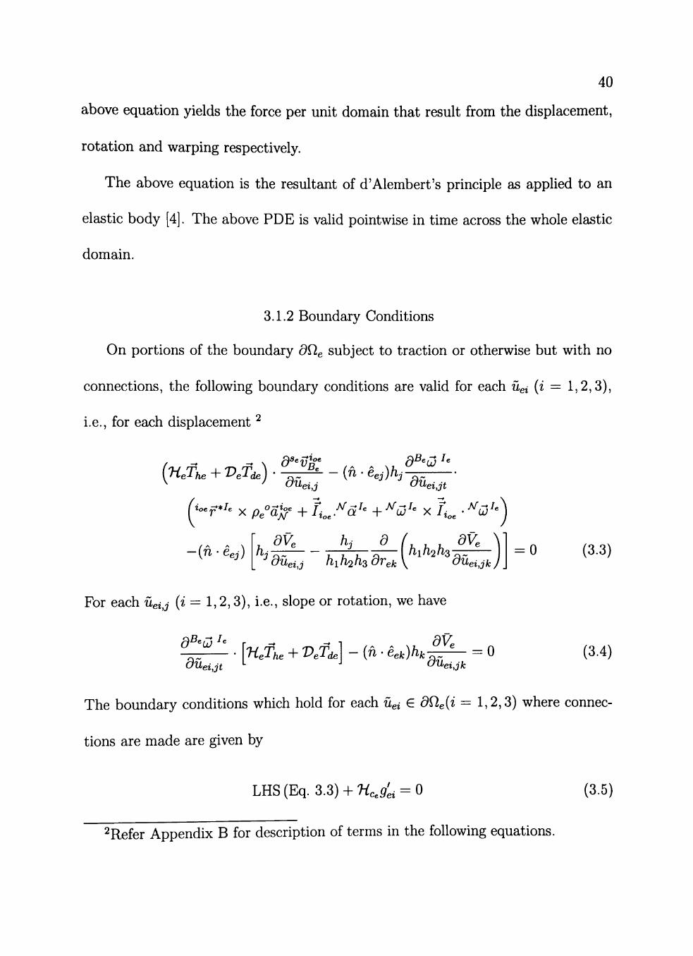
3.1.2 Boundary Conditions

On portions of the boundary d^e subject to traction or otherwise but with no

connections, the following boundary conditions are valid for each ei (i = 1,2,3),

i.e., for each displacement ^

{nefhe + VeTde) ' " ^ ^ - (u • éej)hj OUei,j OUei,jt

-(n-Cej) ^ dVe _ _hj__9_(h,h2hs-^ ^ d eij hih^hsdrekX ^ d ei,jk,

= 0 (3.3)

For each ei,j (i = 1,2,3), i.e., slope or rotation, we have

d^^u^^ r . .^ _ ^ 1 dV

d ei,jt [Hefhe + Vefde - (n ' êek)hk-^Z^ = 0 ( 3 .4 )

eijk

The boundary conditions which hold for each ei € dQeii = 1,2,3) where connec-

tions are made are given by

LHS (Eq. 3.3) + HcJei = 0 (3.5)

^Refer Appendix B for description of terms in the following equations.

41

Also, for every ei,j G dQe{i = 1,2,3), the boundary condition is given by

LES{Eq.3.4)-\-HcXi = 0 (3.6)

The terms p^ and fc^ are as explained in Appendix B.

3.1.3 Impact Equations

The impact process is modeled through the equations presented by Barhorst

[4, 5, 6, 11] and their general form is as shown below. On integrating equation 3.1

over the time of impact and taking the limit of the resulting equation with time

tending to to, the time of impact, the following momentum equation (Eq. 3.7) results

[4, 5, 11]. The post-contact/impact velocities for the ordinary coordinates, i.e., the

rigid bodies can be evaluated from the foUowing equation

r l ^^n

\,.-[fr-{Hr{t:)-Hr{t-))] d^Û^^

dSn

+ E \ ^ \ t t ' [Ã - {Le{tt) - Le{tã))] dSn

,^-[fe-{He{tt)-He{t-))] > = 0. (3.7) dSn

The individual terms in Eq. 3.7 are defined in Appendix B. The physical significance

of the above equation is that it is the amount of momentum required to bring the

system into conformance with the constraint. The partial velocities are evaluated at

í+ because, in the case of rigid-flex impact, the bodies do not separate immediately

after impact as in the case of a rigid-rigid impact. Instead they stay connected

42

the instant after impact. This phenomenon is used to calculate the post-impact

velocities using the equation above. AIso, note that the partial velocities are only

functions of positions and not velocities.

When the field equation (Eq. 3.2) is integrated over the period of impact, and

the limit taken as the time tends to the time of impact.

HePhe + VePd. - Tflu (>^*^^ ( C ) " V*^« ( í ,"))] ^ffíT*-'fî,

d ei,t tt

1 d

hih^h^ dr, ej

d^^u u Uu 1 r -• -• hih^hs^ \i+ ' \HeThe + VeTde

dUei,jt ° L

- {^-r'- X mu {^v'- {tt) - V^^ {t-))

+ 4e-(^-M^o")-'^-M^o")))]} 1 /-)

-^Hc^G'ei - , , , ^ {hih^hHceK'ei) = 0 (3.8) hih^hsdrej^ '

results. The interconnection terms G'ei and K'ei are defined in Appendix B. The

terms used in the above equation are also explained in Appendices A and B. The

above equation is valid pointwise in time over the whole domain of the elastic body.

3.2 The Two-Link Flexible Planar Manipulator

The general form of the equations of motion will be used to develop equations of

motion for a two-Iink planar fiexible manipulator as shown in figure 3.1. A physical

model for the above mentioned manipulator that undergoes free-flight, contact-

impact and constrained motion has been built and is elaborated on in Chapter

V.

43

For reference, a brief description of each of the individual bodies in the manip-

ulator is given below.

1. First rigid body {RBi) - The rigid body (Figure 3.2) that is connected to the

output shaft of the base motor-gearbox (also referred to as first body in the

system of bodies or first hub).^

2. First elastic body - The beam that is connected to the first rigid body (also

referred to as second body in the system of bodies or first elastic body).

3. Second rigid body {RB^) - The rigid body (Figure 3.2) connected to the outer

end of the first beam. This body also contains the second motor-gearbox

assembly that drives the second beam (also referred as third body in the system

of bodies).

4. Third rigid body {RB^) - This is the body (Figure 3.2) that is attached to the

output shaft of the second motor-gearbox (also referred to as fourth body in

the system of bodies or second hub).

5. Second elastic body - This is the beam that is connected to the end of the third

rigid body (also referred as fifth body in the system of bodies or second elastic

body).

6. Fourth rigid body {RB4) - This rigid body (Figure 3.2) is attached to the outer

end of the second beam and houses the tool that impacts the environment or

workpiece (also referred as sixth body in the system of bodies).

^Note difference between m^^ rigid body and n^^ body in the system of bodies.

44

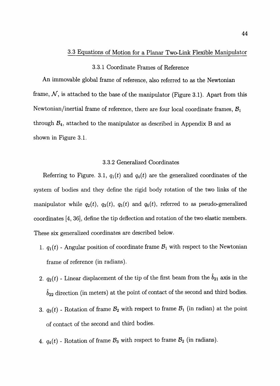
3.3 Equations of Motion for a Planar Two-Link Flexible Manipulator

3.3.1 Coordinate Frames of Reference

An immovable global frame of reference, also referred to as the Newtonian

frame, A/", is attached to the base of the manipulator (Figure 3.1). Apart from this

Newtonian/inertial frame of reference, there are four local coordinate frames, Bi

through B^j attached to the manipulator as described in Appendix B and as

shown in Figure 3.1.

3.3.2 Generalized Coordinates

Referring to Figure. 3.1, qi{t) and q^^t) are the generaUzed coordinates of the

system of bodies and they define the rigid body rotation of the two links of the

manipulator while q^^t), qs^t), q^^t) and qe^t), referred to as pseudo-generaUzed

coordinates [4, 36], define the tip deflection and rotation of the two elastic members.

These six generalized coordinates are described below.

1. qi{t) - Angular position of coordinate frame Bi with respect to the Newtonian

frame of reference (in radians).

2. q2{t) - Linear displacement of the tip of the first beam from the 621 axis in the

622 direction (in meters) at the point of contact of the second and third bodies.

3. qs^t) - Rotation of frame B2 with respect to frame Bi (in radian) at the point

of contact of the second and third bodies.

4. 94(0 - Rotation of frame Bs with respect to frame B2 (in radians).

45

5. q^{t) - Displacement of the tip of the second beam from the 631 axis (in meters)

at the point of contact of the third and fourth bodies.

6. qQ{t) - Rotation of frame B4, with respect to frame B3 (in radian) at the point

of contact of the third and fourth bodies.

3.3.3 Active Forces and Torques

The active forces F^ on each body are

(3.9)

idxnfís (3.10)

(3.11)

(3.12)

iidxsiûs (3.13)

(3.14)

and the active torques are

f i = T,ns (3.15)

f2 = 0 (3.16)

fs = -T2fi3 (3.17)

n = T^fis (3.18)

f, = 0 (3.19)

f6 = 0 (3.20)

Fi =

P2 =

Ps =

PA =

P5 =

Pe =

-mig fis

rLu -P29 /

Jo

-ms9 fis

-m9 ^3

/•L21

-P59 /

-rriQg fis

46

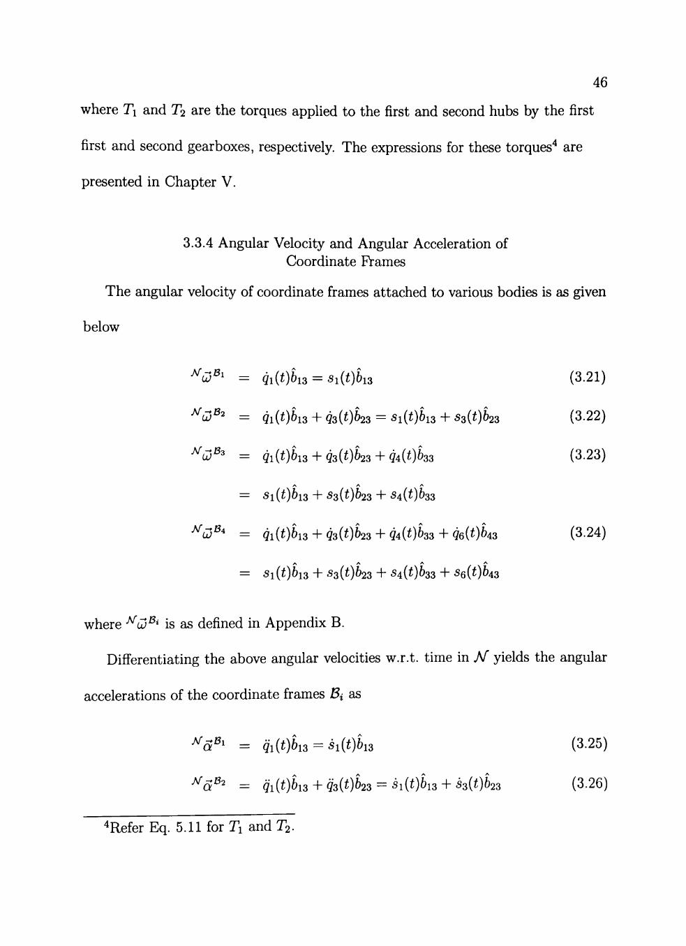
where Ti and T^ are the torques applied to the first and second hubs by the first

first and second gearboxes, respectively. The expressions for these torques"* are

presented in Chapter V.

3.3.4 Angular Velocity and Angular Acceleration of Coordinate Frames

The angular velocity of coordinate frames attached to various bodies is as given

below

^ ^^ = qi{t)b,s = si{t)hs (3.21)

^Û^' = qi{t)b,s-^ q3{t)b23 = si{t)hs-^ ss{t)b2s (3.22)

^ ^' = qi{t)hs-^ q3{t)b2s-^ Ut^hs (3.23)

A A ^

= si{t)bis + 53( )623 + SA{t)bss

^Û^' = qi{t)hs-^ q3{t)b2s-^-q4{t)bs3 ^ q6{t)h3 (3.24)

= si{t)bis + 53(0^23 + 54(0^33 + SQ{t)hs

where •^û^' is as defined in Appendix B.

Differentiating the above angular velocities w.r.t. time in AT yields the angular

accelerations of the coordinate frames Bi as

A^^^i = qi{t)bis = si{t)bis (3.25)

^ã^' = qi{t)bis + q3{t)b23 = si{t)bis + ss{t)b2s (3.26)

4Refer Eq. 5.11 for Ti and T .

47

^a^^ = qi{t)bis + qs{t)b23-^ qA{t)bs3 (3.27)

= 5irø^i3 +53(0^23+ 54( ) 33

^ã^' = qi{t)bis-\-qs{t)b23-^ qA{t)bs3-^ q6{t)h3 (3.28)

= 5l(í)^13 + 53(í)Í23 + 54(0^33 + 56(0^43

where ^ Q ^ * is as defined in Appendix B.

3.3.5 Position, Velocity and Acceleration of Special Points

A point of interest, called a special point [5, 6, 9], 5pi, is selected for each body

with reference to which the properties of that body are written. For the system that

is being studied in this work, the position of the center of gravity is selected as the

special point for each rigid body in the system. The origin of the elastic body in

its local coordinate frame is taken to be the special point of interest for each elastic

body. The absolute position of the special point of each body is denoted by "f^^',

where i denotes the i^^ body and the position vector of an intermediate frame of

the elastic body is referenced as ^^f^^ where j is the number of the coordinate

frame associated with each elastic body and i is as defined above. With reference to

Figures 3.1 and 3.2, the position vector of each of the special points in the system

of bodies is as given below^

^Refer Figure 3.2 for explanation of variables rx^cgi^ etc.

48

o^Sv, ^ ''f^^+r,,cgMl + ry,cgM2

^'fÍl = Xiibii-^ i2{Xii,t)bi2

o^sps = ^f^'^Libii^q2{t)bi2^r,cg,b2i^rycgM2

rj/ = r ^ + rot^b^i + rotyb^^ + r jicg ^ i + ^ 054 32

"fP"" = ^f^'-\-r^,cgMl-^ry,cgM2

^°Vg = a;2i63i + îÍ22(a^3i,í)^32

o^spe ^ ^f^'-^L2bsi + qÁt)hs2 + r:,cg,ki + rycgJ)A2. (3.29)

Differentiating the above position vectors once and twice w.r.t. time in A/" yields

absolute {°v^^') or local {^""^VQ^) velocities and absolute {""a^') or local (^°^a^0

accelerations of the special points.

3.3.6 Acceleration of Center of Gravity of the Bodies

The absolute accelerations of the center of gravity (c.g.) of the bodies in the

system are required to calculate their inertia forces. For the rigid bodies of the

manipulator, the special points were selected to be at the c.g. of each rigid body,

and hence the set of expressions for accelerations from section 3.3.5 hold, i.e.,

and for the elastic bodies, the absolute acceleration of the intermediate frame is

^ã^^=^ã'J^+''^ãi; (3.31)

49

3.3.7 Displacement of Elastic-Bodies

The elastic-bodies, assumed to be Euler-Bernoulli beams, are treated as can-

tilever beams with tip masses in the local coordinate frame. The displacement of

these beams with respect to their local coordinate frame is assumed to conform to

field displacements i^^Xn.t) for the first beam and 22{x3i,t) for the second beam,

where

i2{xiut) = (I)q2{xii)q2{t)-\-(l)q^{xii)qs{t) (3.32)

22{X3ht) = (t)q,{Xsi)q5{t) + (t>qe{Xsi)q6{t) (3.33)

and q2{t), qs{t), q^^t) and q^^t) are as defined before. The coefficients of the pseudo-

coordinates (also refered to as shape functions) in equations 3.32 and 3.33 are

f-2xii^ , 3a;n^ 092(^11) = r 3 +

093 (^ i i ) =

Li' Li''

Xu^_Xi^

Li' Li

. . . f-2xsi^ ^Sxsi"^ (pqs{X3l) = I . 3 + 7 ; ^

0,e(-3i) = ( l ^ - ^ ) - (3-34)

With reference to figure 3.3, xn and 2:31 are the distances of an intermediate frame

along the 611 and 631 directions respectively. The above Hermite shape functions

satisfy the essential boundary conditions of the beams, as seen in their local frames.

50

3.3.8 Strain Energy Density Function

The strain energy density (per unit length) function for the elastic-bodies,

namely the beams, relates to the measure of energy stored in the beams due to

bending. This function is derived based on the assumption that the beams are

Euler-Bernoulli beams and is

V^.\Ea,{pØ^ (3.35)

where i = 1 and 2 for the first and second beams, respectively. Ei and U are the

modulus of elasticity and the area moment of inertia of the respective beams. AIso

to note is that only small defiections are assumed and non-Iinear effects due to large

deflection are ignored. But, large deflections can be easily accommodated in the

model by modeling the beam using higher order beam theories.

3.3.9 Inertia Forces and Torques

The inertia forces { r) and torques (X) [4, 5, 6, 9] acting on each rigid body of

the manipulator are given by ^

/ , = mr'^ã*^ (3.36)

/ , = ^ - f * ^ x m / a j : , ^ - 4 . - ^ a ^ ^ - ^ í l 5 ^ ^ x 4 , . ^ ã ; ^ ^ (3.37)

where r denotes the r^^ rigid body and for the elastic bodies by

e = í mi^'ã*J^d^e (3-38) jQf

^Refer Appendices A and B for explanation of terms.

51

/e = ^ [ °'=r °'= X m//aj:/'=+

^ep /e X mifã;}- + 4 ^ . ^a^'^ ^^u'^x fi^^ •^u''^^ dQe- (3.39)

The subscript e denotes the e ^ elastic body. In the case of Euler-Bernoulli beams,

the rotary inertia tensor I^^^ equals zero. In the above equations, m/^ is the mass

per unit domain and for the two link flexible manipulator, it is the mass per unit

length and ^a^" is the absolute acceleration of a differential mass in the domain,

3.4 Equations of Motion Governing Free Flight

Having deflned the required positions, velocities, accelerations, forces and

torques that affect the system of bodies, the equations of motion (EOM) for the

two-Iink flexible manipulator are derived below. Before developing the equations of

motion, the two independent regularized or generalized speeds, Si{t) and s^^t), and

the pseudo-generalized speeds, s^^t), Ss{t), s^^t) and SQ{t), of the manipulator are

defined as

Si{t) = qi{t) (3.40)

where i = 1,2,. . . , 6 . The time derivatives of the field displacements denoted as

i2{xii,t) and 1^22( 31,0 are

Ui2{Xiut) = ^2{t)^-J^ + -^j^Ss{t)^j^- —

Ui2{Xii,t) = ^ 5 r ø ( - ^ + ^ l + ^ 6 ( í ) ( ^ - ^ ) . (3.41)

52

The equations of motion that govern the generalized coordinates are given by the

ordinary differential equation (ODE), Eq. 3.1, and those for the field displacements

are given by the partial differential equation (PDE), Eq. 3.2.

3.4.1 Ordinary Differential Equations of Motion

Using equation 3.1, the ODEs governing qi{t) and q^^t) are

^ifl-'^^i«--.i ^ift-íh^ifl-íi

^ l A - ' . h ^ P - ^ J Êg!. (,. _ /.|, 2 | ^ . [fl _/.] = „ ,3.«,

and

5 Î l f i - S h ^ r . - * l = f l f i - % ^ l « - * l Ég:.p_r.].»^.Ifl_/.]

53

respectively.

3.4.2 Elastic Partial Differential Equations of Motion

The Eq. 3.2 yields the PDE's for the each of the field displacements. The

equations that govern the field displacements i2{xii,t) and 22{x3i,t) of the first

and second elastic bodies respectively are

\-mi,^ã;f^ d'^v'^l ^2 f QY^

d i2{xii,t) ^a;ii2 \d '(2{xii,t) = 0 (3.44)

and

where ^^2(^12, t) represents the second derivative of the function Í2{XÍ2, t) w.r.t. the

spatial variable. Equations 3.44 and 3.45 when recast in their weak form^ allow

solutions for coordinates q^^t) and qs{t) and q^^t) and qQ{t) of the first and second

elastic bodies. The terms G'd and K'd from Eq. 3.2 do not contribute to the above

PDE's as there are no connections in the domain of the elastic beams.

3.4.3 Boundary Conditions

The boundary conditions for tip displacements of the beams are given by Eq. 3.3

and by Eq. 3.4 for tip rotations. AIso presented in Appendix B is the methodology

to evaluate the boundary conditions.

' Refer section 3.7.1.

54

The ordinary and partial differential equations developed above constitute the

minimum set of differential equations that describe the motion of the manipulator

in free fiight. The next section is devoted to developing the equations of motion of

the manipulator in the constrained motion regime.

3.5 Equations of Motion Governing Constrained Motion

The manipulator is said to be in the constrained motion regime when the tool

attached to the tip of the manipulator tracks or moves along a surface. The re-

sulting constraint force is calculated through a pseudo-coordinate qj^t), which is a

virtual penetration of the manipulator tool into the constraint surface. AIso, an-

other coordinate qs{t) as shown in Figure 3.4 is introduced to help form a vector

loop equation {VLE) [5]. This vector loop equation is used to arrive at the non-

holonomic constraint that governs the manipulator when it comes into contact with

its environment.

3.5.1 The Non-Holonomic Constraint

The first step in developing the non-holonomic constraint is to write the VLE

for the manipulator as follows

VLE = ""fp + toolMi + toolybA2 - qi{t)ni - q%{t)fi2 + hfii = 0. (3.46)

where "f^f is the position to the c.g. of the sixth body and tool^ and tooly are as

shown in Figure 3.2. Now, considering q^^t) to be the dependent coordinate, the

55

VLE wiU be used to solve for q^^t) in terms of the other coordinates. To do that,

the dot product of Eq. 3.46 is taken with vectors ni and n^ oi M to get

Ci = VLE • fii = 0

C2 = VLE'h2 = 0.

(3.47)

(3.48)

The above equations are transcendental and are solved using the Newton-Raphson

method. Differentiating Equations 3.47 and 3.48 w.r.t. time in J\í gives

Ci =

C2 =

dt

dt

{VLE • ni) = 0

{VLE • n^) = 0

(3.49)

(3.50)

and rearranging the terms results in velocities s^^t) and Sg^t) in terms of the other

generalized coordinates and speeds as shown below

S4{t)

S8{t)

^ 1 - 4 ^ 1 - 8

a «4

rhss^ )

C2 rhs

rhs 38

= [J] -1

'S4

rhs ss

(3.51)

(3.52)

where

Ci,^ is the coefficient of s^^t) in Eq. 3.49,

Ci,g is the coefficient of Sg^t) in Eq. 3.49,

C2, is the coefficient of s^^t) in Eq. 3.50,

C2 is the coefficient of Ss^t) in Eq. 3.50,

rhss, comprises terms in Eq. 3.49 not associated with s^^t) and Sg^t) and

56

rhsss comprises terms in Eq. 3.50 not associated with s^^t) and sg^t).

Similarly, the constrained accelerations á^^í) and sg^t) are given by

s,{t) )

ss{t) J

- 1 í rhss^ 1

= [Jr{ rhs S8 J

(3.53)

where rhss^^ consists of terms in J^Ci = 0 not associated with 54(í) and Ss{t) and

rhss^ consists of terms in ^ C ^ = 0 not associated with 54(í) and Sg^t).

3.5.2 Force of Constraint

When the manipulator tool comes in contact with the constraint surface, the

pseudo-coordinate q^^t) comes into play. The force, Pc, that is required to bring the

manipulator into conformance with the constraint [5, 37], i.e., for qj^t) to be zero is

given by Eq. 3.1 as

Fr = E r

E

' d°v -*S Pr 'M

ds-j -,S

d°v Pe 'M

dsj

'r]^^:^-[^r-Jr]

-L +

ds7

d^u^^ dsi

[fe - Je] (3.54)

L.e., the partial velocities are taken w.r.t. the fictitious speed Sj^t).

When the manipulator undergoes constrained motion, an opposing force in the

form of friction acts on the tool. Hence, the expression for the force acting on that

rigid body (namely, the sixth body) is given by

i^6 — —P'{'^sign) n2 (3.55)

where n is the kinetic coefficient of friction and Vsign is the sign of the velocity vector

of the tip of the tool in constrained motion.

57

Eq. 3.42 provides the ordinary differential equation of motion in the constrained

mode that governs qi{t) when 54(t) and 54(t)^ are substituted for from Equations

3.52 and 3.53, respectively. The partial differential Equations 3.44 and 3.45 and

boundary conditions referred to in section 3.4.3 are valid in the case of constrained

motion also when the constrained quantities are rewritten in terms of the indepen-

dent coordinates, velocities and accelerations. Note that in the constrained mode,

q4{t) and qg^t) are solved using the Newton-Raphson method through transcendental

equations 3.47 and 3.48 at each time step of the numerical integration process.

3.6 Momentum Equations on Contact/Impact

At the instant the manipulator's tool comes into contact with the constraint sur-

face, a non-holonomic constraint is instantly enforced. This fact is used to derive

the post-impact initial conditions for constrained motion. The following equations

result in the generalized algebraic momentum equations which when solved simul-

taneously, yield post-impact velocities. The algebraic momentum equations for the

two-Iink flexible manipulator are

£ I ^ i ' î • [ ' - (^^(*°' - ^^^^ô))] ' &j^V^''

dsi

^ ^ | . j . [% - {Hr{tt) - H,{t-))\ dsi

+ E(¥^b-[Ã-(£e(tí)- e(í„-))] dsi

^These quantities will also be referred to as constrained quantities.

58

ds Att ' [ í - {He{t:) - He{t-))] I = 0 (3.56)

for Si{t), with

[-»/. (>-*'' (C) - V ' ' (t„-))] • ^ l.í= 0 (3.57)

for íii2(a;ii,í) and

[-m/. (>-^= (C) - >-'= (í„-))] • ^ l.í= 0 (3.58)

for •1622(3: 31, ^). Equations 3.57 and 3.58 are valid pointwise in space.

It should be noted that pre-contact positions are used in calculating the partial

velocities in the impact-momentum equations but the post-impact velocity (at time

to'^) is written to conform to the constrained configuration. The reason being that

over the time of impact, the position of the manipulator is considered to remain

stationary.

In the derivation of the equations of motion for the flexible manipulator above,

the equations governing the field displacements were presented in partial differential

equation form. That form retained the spatial and temporal variables. In the

following section, the weak form of these PDE's are derived which resolves the

spatial variable and yields the equations of motion as a function of time only.

59

3.7 Generation of the Weak Form

3.7.1 Weak Form of Partial Differential Equations of Motion

The weak form of the PDE's is generated based on the Ritz [58] methodology.

The partial differential equation from section 3.4.2 governing i2{xii,t) is

\-m,°n."'] ^'^t' ^' / dV, \

[""' "^\• au;;^) -ã ;?iãû^(w)J='' ^^''^ and that governing 22(2 31, ) is

1-^,"^'^] ^ " ^ ' ^ ( ^^' ] 0 í3 6m [ '' "^ J dMx,,,t) - ã ^ [ d Uxsut)) -°- ^^•'"'

To generate the weak form, the above equations are multiplied by a test function

and then integrated over the domain of the elastic body of interest. For the two-

link flexible manipulator, the shape functions in Equations 3.34 will be used as the

test functions for generating equations for coordinates q2{t), qs^t), q^^t) and q^^t),

respectively.

The weak form of the equation of motion affecting q^^t) is derived below using

Eq. 3.59. The test function used is (t)q^ from Equations 3.34. The flrst step is to

multiply Eq. 3.59 with ( ^ ^^^ integrate the resulting function over the domain of

the first elastic body. This results in

/ i[-m,-a;f'] • - ^ - _ ^ f - ^ ) } ^ , . . 0 = 0 (3.61) y n U ' ^-1 d i2{xii,t) dxii^ \du'{2{xii,t))]

i.e.

k U '^' • ^ J ô û i 2 ( i u , t ) dxn''\d '[.,{xn,t)

60

-2^ + ^^\dxn = 0 (3.62) Li Li )

Similarly, when Eq. 3.59 is operated on with (/gg as the test function, and Eq. 3.60

operated on with <^q^ and (^q^ as the test functions, as in Eq. 3.61 the following result

r ' ír^os./.i yg^' g { g i M io U '^' "^J Ôíii2(x„,í) 9x„2\^a«Î2(xn, í ) j /

L _ i i '

•/-3 ír _.r.n Ô» í7k &" 1 dV

l i _ _ ii_]da;„ = o (3.63)

io \ l ^ " ^ J • ÔÛ22(X21,Í) 9X21^ \,a ^'2(X21,t); /

Z | | l ! + 3X211 d^ , = 0 (3.64) 2 - 2 /

7o \ L ^ 2 ^ ^ J aé22(x2i,í) a:z:2i2V5n'2'2(:i^2i,í) , 3 ^_ .2

L ^^.^^]dx2i = ^ (3.65)

Pi is the mass density per unit length of the elastic bodies. Equations 3.62

through 3.65 are the four ordinary differential equations governing the four pseudo-

coordinates. These four equations along with Equations 3.42 and 3.43 and the six

kinematic ODE's constitute the twelve first-order differential equations that need

to be solved in time to predict the motion of the fiexible manipulator.

In the case of constrained motion, the equations developed for the independent

speed si{t) and the pseudo-speeds s^^t), ss{t), s^^t) and SQ{t) in unconstrained

motion hold when the dependent velocity {s^^t)) and acceleration {s^{t)) are substi-

tuted for in terms of the other five independent quantities. The dependent coordi-

nate {q^{t)) is evaluated through Equations 3.47 and 3.48 using the Newton-Raphson

61

method at every integration step. The above five equations of motion solve for

the independent coordinates and the dependent coordinate is solved for using the

constraint relation, VLE, at each integration step.

3.7.2 Weak Form of Momentum Equations

Equations 3.57 and 3.58 are the two equations in space that affect the pseudo-

coordinates when the manipulator undergoes contact/impact with its environment.

The weak form of these equations are generated as before with test functions øg ,

093 5 (I>q5 and (j)qQ (Eq. 3.57 is operated on by (pq^ and øgg and Eq. 3.58 by ( g and (f^q^).

The weak form of Eq. 3.57 and 3.58 for q^^t), qs{t), q^^t) and q^^t), respectively are

/,{[-^.(VM*í)->-M*í))]-1£^bl >(l)q^dxii = 0 (3.66)

QS2 ^ i^.

L \-~p^ ( ' *' (' )" ' *' (' ))] • ^ ^'^ r" ' " ^' '- ^ «5 „-r lo2 d%lv

L [-^ ^'^'^ ( ) - ^*' (''))! • r '- r ' ^ =' ^'-''^ l{[-P2{>-H^^)->^'Hm -^ lí+

5^22 •056^X21 = 0. (3.69)

The boundary conditions associated with equations 3.66 through 3.69 are

(BC^o^n), = (3-70)

^ l . í • [- ( .(tí) - Ut:))] + ^ L í • [- iUi) - U:))]

+ ^ | , j . [- (£,(C) - i2(t;))] + ^ l t • [- {H.{tt) - H,{t;))]

+ ^ l , , . [_ {Utt) - Ut;))] + l , • [- {H.{tt) - H3(*;))]

+ ^ l . î • [- (£ ('í) - ^ ('ô))] + ^ l ' í • [- ( (*í) - ^ (*°')]

62

|,j . [- (£5(tJ) - U{t-))] + - ^ l , . . [- {H,{tt) - H,{t-))]

^ l , . . [- (Le(tí) - £a(t„-))] + ^ L j • [- (He(C) - H,{t;))]

dSi "' L \ •'^0, u. o / ; j ^^.

^^'°l í (L(t+\ L(t-))] + ^°' -^l<f[-(Mt„)-í '6(t„)Jl + - ^

where i = 2,3,5 and 6 respectively.

The above integrals were expedited with the use of Mathematica [2] which allows

symbolic generation of equations. These equations were later solved numerically by

rewriting them in FORTRAN.

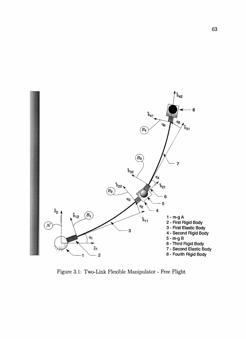
63

1 - m-g A 2 - First Rigid Body 3 - First Elastic Body 4 - Second Rigid Body 5 - m-g B 6 - Third Rigid Body 7 - Second Elastic Body 8 - Fourth Rigid Body

Figure 3.1: Two-Link Flexible Manipulator - Free Flight

64

Second Rígid Body Fourth Rigid Body

Figure 3.2: Rigid bodies of manipulator

65

A

b i2

'01

Figure 3.3: Coordinates Describing Shape of Beam

66

Figure 3.4: Two-Link Flexible Manipulator - Constrained Mode

CHAPTERIV

RIGID BODY MODEL

Presented in previous chapters was a high fidelity theoretical model for a two-

link flexible manipulator which is a non-Iinear model encompassing the dynamics

of all the elements present in an actual system as described in the Chapter III.

Presented in this chapter is an approximate model of the flexible manipulator,

where the flexible links are modeled as rigid bodies. In this model, the elastic

nature of the flexible member of the flexible manipulator is approximated through a

torsional spring placed in between the hub and the (rigid) beam. This simpliflcation

leads to the reduction of the degrees of freedom from six to four. Although the

beams are modeled as rigid members, the rigor of the model is maintained by

accounting for all the other non-Iinearaties and dynamics that were included in

the complete model in Chapter III. The comparison of the dynamics of the rigid

body model elaborated below with that of the full flexible model developed earlier

is the third major contribution of this research (the second major contribution is

the experimental verification presented in the next chapter).

The reason for the development of this low-fidelity model is to see how much

of the actual dynamics the lower order model can pick up and also to see if this

model is suitable for control applications. The control application refers to the

applicability of the low-fidelity model in the development of control laws to control

the motion of the corresponding flexible manipulator.

67

68

4.1 Coordinate Frames and Generalized Coordinates

The system of bodies of the two link rigid manipulator are as shown in Figure

4.1. There are four frames of reference, Bi through 64^ riding with the manipulator

and one fixed Newtonian frame of reference, J\í. The Newtonian frame of reference

is fixed in space and has its origin at the pivot point of the first rigid body.

For this rigid model, four generalized coordinates, qi{t) through q^^t), are re-

quired to describe the configuration of the system in space. The coordinate qi{t)

is the angle that frame Bi makes with the Newtonian frame TV and, 52(0 is the

angle between coordinate frames Bi and B^. Similarly, qs{t) and ^^(í) are the angles

that coordinate frames Bs and B4 make with frames B2 and Bs, respectively. The

generalized speeds of the rigid model are defined as

Si{t) = qi{t) (4.1)

where i= 1,2,... ,4.

4.2 Active Forces and Torques

The active force Fr on each rigid body is

Fi = -miQns (4.2)

where z = 1,2,..., 6 and the active torques^ are

fi = Tins + Kiq2{t)fi3 (4-3)

iRefer Eq. 5.11 for Ti and T .

69

T2 = -Kiq2{t)fis (4.4)

fa = -T2n3 (4.5)

Í4 = T2 ns + K2 q4{t) ns (4.6)

T5 = -K2q4{t)ns (4.7)

f6 = 0 (4.8)

where K^ are from the torsional springs modeling the elasticity of the beams and Tj

are torques from the gearboxes.

4.3 Angular Velocity and Acceleration of Coordinate Frames

The absolute angular velocity (^o;^'') of coordinate frames Bi through B/Í re-

spectively, are

^ ^^ = qi{t)bis = si{t)bis (4.9)

^ ^' = qi{t)bis-\-q2{t)b23 = si{t)bis-^ S2{t)b2s (4.10)

^Û^' = qi{t)bis + q2{t)b2s + q3{t)bs3 (4.11)

= Sl{t)bis + 52(0^23 + 53(0^33

^ ^' = qi{t)bis + q2{t)b23 + q3{t)b33-^ qÁt^hs (4.12)

= Si{t)bis + 52(í)^23 + 53(0^33 + 54( )643-

When the above angular velocities are differentiated w.r.t. time in J^, the angular

accelerations (^a^'-) of frames Bi through B4 result, respectively, as follows

AT^fíi qi{t)Í>is = h{t)bi3 (4-13)

70

^ a ^ ^ = gi(í)6i3 +92(^)623 = 5i(í)6i3 +52(0^23 (4-14)

^ã^' = qi{t)bis + q2{t)b23 + q3{t)b33 (4.15)

= Si{t)bis + S2{t)b23-^ Ss{t)bss

^ã^' = qi{t)bi3 + q2{t)Í23 + q3{t)bs3 + Ut)k3 (4.16)

= 5i(í)6i3 + 52(0^23 + 53(0^33 + 54(0^43.

4.4 Position, Velocity and Acceleration of Special Points

As discussed in section 3.3.5, a special point is chosen for each body, and for

the rigid manipulator, the position of the center of gravity of each rigid body is

considered to be the special point. The absolute position of these special points(5pi)

are

ofSpx ^ rxic5i^ll + î yicgx6i2

ofSp2 ^ ^ f ^ ^ + r , , e 5 i ^ l l + r,,e,i^l2 + Y^21

o^Sp, ^ ^f^'-^^b2l + r^cgÅl + rycg,b22

o^Sp4 ^ AífBs ^ ^^^^^21 + rOÍy622 + r^c.cgM + ^ 1^54^32

o^Sps ^ ^f^'^r^,cgM+ry,cgJ)32 + ^b41

o^Spe ^ ^f^^ + ^b4i+r,cgekl + rycgM2 (4-17)

71

where Li and L^ are the lengths of the first and second beams, respectively. Dif-

ferentiating the above position vectors w.r.t. time {t) in J\í once and twice, respec-

tively, yields the absolute velocity ^v^^'' and acceleration ^a^^'" of the special points

( r = l , 2 , . . . , 6 ) . 2

4.5 Acceleration of Center of Gravity of Rigid Bodies

The center of gravity of each of the rigid bodies was selected as their special

point and hence, the acceleration of the center of gravity is that of the respective

special point, i.e.,

^ã*'=-^ã^Pr (4.18)

where r = 1,2,... ,6.

4.6 Inertia Forces and Inertial Torques

The inertia forces (J;) and torques (^) [4, 5, 6, 9] acting on each rigid body of

the manipulator are given by

ír = mr^'d*^ (419)

l = '-f*^xmr'ã;f-l^^-''ã''^-^u^^xt^^^^ ^^ (4.20)

where r = l , 2 , . . . , 6 . The terms in the above equations are explained in Appendices

A and B.

^The subscript r denotes the r ^ rigid body

72

4.7 Equations of Motion Governing Free Flight

With the required positions, velocities, accelerations, forces and torques that

affect the system of rigid bodies defined in the previous sections of this chapter, the

equations of motion for the case where the manipulator is in free flight is derived

below. The set of flrst-order ordinary differential equations governing each qr{t),

where r is the r* rigid body, is given by Eq. 3.1 as

V^^^" \F r U ^ ^ \f n - n uon + ^ i 7 ^ ' " ^J+~9ir'[^"" ^]" * '

where r = 1,2,..., 6 and n = 1,2,..., 4.

4.8 Equations of Motion Governing Constrained Motion

When the tip of the manipulator comes into contact with an external constraint,

it enters the constrained mode. In this mode, the degrees of freedom reduces from

four to three due to the constraint. Hence, there are only three independent gen-

eralized coordinates and the fourth coordinate is found though the non-holonomic

constraint equation developed below. For the two-Iink rigid manipulator, qi{t), q^^t)

and q4{t) are taken to be the independent coordinates and qs{t) as the dependent

coordinate {qs{t) is arbitrarily picked to be the dependent coordinate).

73

4.8.1 The Non-Holonomic Constraint

The non-holonomic constraint was developed by first writing, w.r.t. Figure 4.2,

the vector loop equation {VLE), which is,

VLE = V^^" + tookb4i + toolyb42 - q^{t)ni - qQ{t)h2 + hûi = 0 (4.22)

where °f ^ is the position of the c.g. of the sixth rigid body and tool^ and tooly

are as shown in Figure 3.2.

The dot product of Eq. 4.22 with unit vectors ni and fi^ results in

Ci = VLE'ni = Q (4.23)

C2 = VLE-fi2 = 0. (4.24)

The above transcendental equations are solved using the Newton-Raphson solution

technique. Differentiating Equations 4.23 and 4.24 w.r.t. time in AT gives

^d Ci = --{VLE'ni) = 0 (4.25)

dt ^d

C2 = -^{VLE-n2) = 0 (4.26) dt

which when rearranged as follows results in the expression for the dependent velocity

S3{t)

^ l a a ^ 1 ^ 6

^S3 ^se j

rhss3

(rhSs3

] (4.27) r/i5.

S3{t)

S6{t)

= lJ]-'{ } (4.28)

'S6

rhsse

where

74

Ci,^ is the coefficient of Ss{t) in Eq. 4.25,

Ci,g is the coeffîcient of SQ^Í) in Eq. 4.25,

^2,3 is the coefficient of Ss{t) in Eq. 4.26,

C2,g is the coefl cient of SQ{t) in Eq. 4.26,

rhss^ comprises terms in Eq. 4.25 not associated with ss{t) and SQ{t) and

rhsse comprises terms in Eq. 4.26 not associated with ss{t) and SQ{t).

Similarly, the constrained accelerations ss{t) and SQ{t) are given by

^Át) ] ( rhss, ]

\ = Ur (4.29) SQ{t) ) [ rhss, J

where rhsé^ consists of terms in ^ C i = 0 not associated with ss{t) and SQ{t) and

rhsse consists of terms in ^ C ^ = 0 not associated with ss{t) and SQ{t).

4.8.2 Force of Constraint

When the manipulator tool contacts the constraint surface, the pseudo-

coordinate 95(í) [5, 37] comes into play. The force, Fc, required to bring the manip-

ulator into conformance with the constraint [5, 37] is given by Eq. 3.1 as

-•-^l^l^-r.]^'^-\r.-í] (4.30) dSr, I J dSr:

where r = 1 , . . . ,6 and r denotes the r ^ rigid body. When in constrained mode,

a friction force acts on the tool. Hence, the expression for the force acting on that

body (namely, the sixth body) is given by

FQ = -fl{Vsign) Fc fl2 (4.31)

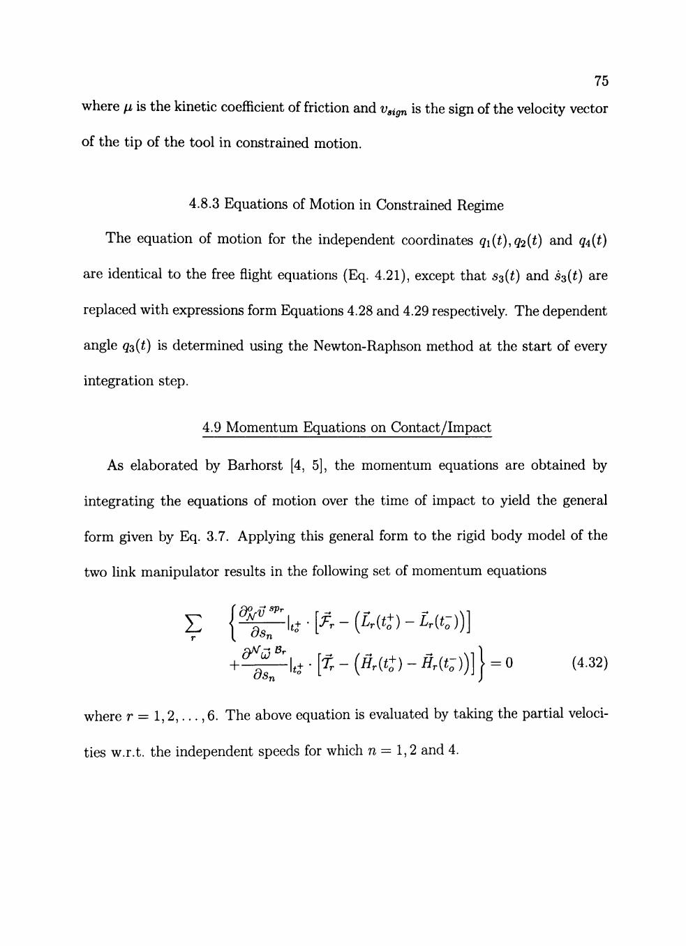
75

where /i is the kinetic coeflacient of friction and Vsign is the sign of the velocity vector

of the tip of the tool in constrained motion.

4.8.3 Equations of Motion in Constrained Regime

The equation of motion for the independent coordinates qi{t),q2{t) and q^^t)

are identical to the free flight equations (Eq. 4.21), except that Ss{t) and ss{t) are

replaced with expressions form Equations 4.28 and 4.29 respectively. The dependent

angle qs{t) is determined using the Newton-Raphson method at the start of every

integration step.

4.9 Momentum Equations on Contact/Impact

As elaborated by Barhorst [4, 5], the momentum equations are obtained by

integrating the equations of motion over the time of impact to yield the general

form given by Eq. 3.7. Applying this general form to the rigid body model of the

two link manipulator results in the following set of momentum equations

dpv'P'

dSn

dSn ' °

E \'^k-[^r-{Lr{tt)-Lr{t-))]

fr-{Hr{tt)-Hr{t-))] > = 0 (4.32)

where r = 1,2,. . . ,6. The above equation is evaluated by taking the partial veloci-

ties w.r.t. the independent speeds for which n = 1,2 and 4.

76

The equations of free flight (Eq. 4.21), constrained motion and momentum equa-

tions (Eq. 4.32) are used to simulate the motion of the rigid manipulator using the

logic explained in Chapter V.

77

Figure 4.1: Rigid body model - Conflguration in free flight

78

21

Figure 4.2: Rigid body model - Configuration in constrained motion

CHAPTER V

NUMERICAL SIMULATION AND EXPERIMENTAL

VERIFICATION

Presented first in this chapter is the development of the FORTRAN code for

simulating the motion of the two-Iink flexible manipulator. The code developed

will then be used to perform numerical simulations of the motion of the manipula-

tor. This motion will encompass all the motion regimes mentioned earlier in this

dissertation namely, free flight, contact/impact and constrained motion. The sim-

ulation results will later be compared with experimental results and the code will

also be used to demonstrate the models adaptability to control applications. Also,

the simulation results of the rigid body model are presented later in this chapter,

5.1 Properties of Rigid Bodies

The geometric and inertia properties of each rigid body were determined using

Pro-Engineer (ProE) [3]. First, each rigid body was modeled (to scale) in ProE.

Then, the density of the individual components of the rigid bodies was deflned.

With all the dimensions and densities, and using ProE's built-in functions, the

inertia tensor about the center of mass of each rigid body was found. Also, the

position of the center of mass of the rigid bodies w.r.t. the respective coordinate

frames were calculated.

79

80

Materials used in the construction of the rigid bodies are discussed in Section

5.5 and their properties are presented in Appendix C.

5.2 Development of Code for the Flexible Manipulator

5.2.1 Free Flight

The six first order differential equations of motion mentioned above were sym-

bolically generated using Mathematica [2, 5]. These six equations when recast in

matrix form yield

i.e..

[lu 16 'Si^ ' rhsi "

7 = \ (5.1)

hi •" 66 J l -56 J l rhsQ .

\h\ {Sj\ = {rhsi) (5.2)

where z = j = 1,2,.. .6, 7« is the inertia matrix and s^ the acceleration vector.

The terms in each row of the inertia matrix is the corresponding coefficient of

the áj's from the six differential equations. The above six equations along with

the six kinematic differential equations constitute the twelve first order differential

equations that model the motion of the two-Iink fiexible manipulator in free-flight.

5.2.2 Constrained Motion

In the constrained regime of motion, the manipulator's degrees of freedom reduce

by one, from six to five. As mentioned earlier in Chapter III, q^^t) is taken to be

the dependent coordinate and is written in terms of the other coordinates through

81

the vector loop equation. Once again, Mathematica was used to generate the five

equations of motion in the constrained regime. The following set of first order

differential equations

[lcij] {sj} = {rhsci} (5.3)

where i = j = l , 2 , . . . , 5 and the subscript c refers to the constrained mode are the

governing equations in the constrained regime. Here again, the terms in UCÍJ] are the

corresponding coefficients of the á^'s of each equation of motion in the constrained

regime. The above five differential equations along with the corresponding five kine-

matic differential equations govern the motion of the two-Iink flexible manipulator

in the constrained motion regime.

5.2.3 Contact/Impact

When the manipulator's tool impacts the constraint surface, the change in mo-

mentum and hence the change in velocities are calculated using Equations 3.56,

3.66, 3.67, 3.68 and 3.69. These equations are a set of five algebraic equations that

look like momii momi5'

'

moms5.

<

R

'Si'

. 5 6 .

> = <

rílSmomi

': >

, r lSmome "

(5.4)

R

82

in matrix form and can be represented as ^

[momij] {Sj} = {rhsmamA • (5.5)

The terms in [momij] are the coefficients of each 5 - from each of the Equations 3.56,

3.66, 3.67, 3.68 and 3.69.

To get an idea of the complexity of the model, each term of the inertia matrix in

the free flight mode was about 200 to 300 lines long of 132 column width FORTRAN

code. In the constrained mode, the length of each term varied anywhere from 300

to 400 lines. AIso, it took about 30 minutes to run a 2.5 second simulation on a

computer with a Pentium Pro 200 MHz processor and 128 MB of memory. On a

500 MHz DEC Alpha server the same process ran ten times faster.

5.3 Development of Code for the Rigid Manipulator

As in the case of the flexible manipulator, the equations of motion for the rigid

manipulator were cast in matrix form and they are as follows.

When the manipulator is in free flight, the Equations 4.21 in matrix form yield

In •'• lu^ (Si 1 (rhsi

LJ41 •

> = <

/44 J l 54 J l rhs4 .

(5.6)

i.e..

[hj]R{sj}ii = {rhSi}j^ (5.7)

^The vector {sj} consists only of post-impact speeds 5i(í+), 52(íj), Ss^t^), 55(í+)

and 56 (íj) .

83

where z = j = 1 to 4, [7^ ] is the inertia matrix, Sj is the vector of accelerations

and the subscript R implies that the equations are that of the rigid manipulator.

The equations governing constrained motion are similar to the above, except

that they yield only three differential equations governing the three independent

coordinates as

[ICÍJ]R {Scj}ii = {'^hSai^R (5.8)

where i = j = 1,2,3 and the subscript c implies that the equations govern the

manipulator in the constrained mode. As in the case of the flexible manipulator,

Equations 5.7 are to be solved along with their corresponding (four) kinematic

differential equations and Equations 5.8 are to be solved along with their (three)

corresponding kinematic differential equations.

The momentum equations for the rigid body model given by equations 4.9 are

recast to yield^

[momij]j^ {sj}j^ = {rhSmcmii}R • (5-9)

The springs that approximate the flexible nature of the beam are calculated as

shown by Huston [33]. The equivalent stiffness, K, of the spring is

K = ^ (5.10)

^The vector {sj},. consists only of post-impact speeds 5i(í+), s^^t^) and s^^t^).

84

where E is the modulus of elasticity of the flexible beam, / , the area moment of

inertia and L, the length of the beam.

5.3.1 Torque Equation

The equation for the torque output of each gearbox for the rigid and flexible

models was obtained from [22] and [45] as

T, = -J^^é{t) - Ce,,.(í) + ^^i^ - "^U^e^At) (5.11) rii tti

where J^q is the equivalent inertia of the motor and gearbox, C^q is the equivalent

damping of the motor and gearbox, Kt is the motor constant, Kb is the back-emf

constant, e^ is the applied voltage, n is the gear ratio and z = 1 for the flrst gearbox

and i = 2 for the second gearbox.

The procedure used to flnd J^q and C^q is discussed in section 5.5.1.

5.4 The Simulation Logic

The numerical simulation utilizes the above equations of motion and momen-

tum equations in their matrix form, in the logical sequence shown in Figure 5.1 to

simulate the motion of the flexible manipulator. The variables and the logic are

explained below.

In the numerical simulation, if the current time {t) is less than the final time

{tf), then, the program enters the integration loop. Initially, the position of the

tip of the tool is found through the function tipjposition and assigned to a variable

dummyi. If this position is less than or equal to five millimeters from the constraint

85

surface, then, the increment in time, delt, is reduced to deltnear; else it is deltfar.

The variable const is a flag which is zero if the manipulator is in free flight and one

if in constrained motion.

When the manipulator is in free flight, a check is performed to see if the tool's

tip has made contact with the constraint surface. If so, then const is set to one and

the momentum equations (Eq. 5.5) are used to calculate the post impact velocities.

If the tool tip and the constraint surface have not made contact, then, const remains

zero and the momentum equations are not accessed.

AIso, when the manipulator is in free flight {const = 0), the vector of state

variables y is assigned to a vector x, and passed to Isoda,^ which solves the equations

of motion {eom) in free flight . After performing the integration, the vector y is

updated using the values of x that Isoda returned in the subroutine XtoY.

If the manipulator is in the constrained regime {const = 1), then the program

steps to the statement if {swsignold .eq. 0) swsignold = switch{y,nc,t). When

in free flight, swsignold = 0. The function switch calculates the force of constraint

and returns a value of 1 if the constraint force is greater that zero and - 1 if the

force of constraint is negative. The value of switch from the previous time step is

stored in swsignold and the current value in swsign. Now, if the numeric value of

the force of constraint goes through zero, it implies that the manipulator has lost

Hsoda [56] is a numeric solver with adaptive step size for solving a set of stiff differential equations.

86

contact with the surface. If the product {swsign * swsignold) is greater than zero,

then, the manipulator tip is on the constraint surface and if {swsign * swsignold)

it is less than zero, then, the manipulator's tip looses contact with the surface and

const is reset to zero and the manipulator enters the free flight mode.

When the manipulator is in the constrained regime, the values of y are mapped

on to xc, which reflects the order of the constrained system, and the set of Equations

5.3 is integrated using Isoda. On completion of the integration, the values of the

dependent coordinate and velocity are updated, in the subroutine update (which

uses Newton-Raphson [70] method to solve for the dependent coordinate), and maps

back to y.

Based on the value of const, the equations of motion governing free flight or

constrained motion are integrated at the next increment in time until t = tf.

Using the logic discussed above, a simulation of the two-Iink flexible manipulator

was performed for various sets of initial conditions, the results of which are presented

in Section 5.6.

5.5 Experimental Setup

The physical model of the testbed has two permanent magnet DC motors and

each drives a planetary gear box. The first motor-gear box combination {m-g A)

drives an aluminum beam through a rigid hub {RBi)'^ as shown in Figure 5.2. At

"^RB implies Rigid Body.

87

the end of this beam is a another rigid mass {RB^) onto which the second motor-

gearbox combination {m-g B) is mounted. A second aluminum beam, has on

one end a rigid hub {RBs) driven by m-g B and on the other end a tool {RB4)

which impacts with a rigid surface and then moves along the impact surface in the

case of constrained motion. The second motor-gearbox combination and the tool

are mounted on air bearings which fioat on an aluminum table. The air bearings

provide near zero frictional forces. Air at 60 psi keeps the air bearings afloat.

The angular position of each arm is tracked using digital encoders mounted on

the end of the motors. This reflects the actual motion through the gear ratio of

each arm of the manipulator. Accelerometers measure the acceleration at various

points along the beams as seen in Figure 5.2. For further reference, the point of

attachment of the accelerometers at the mid-point of the first beam, the second rigid

body, the mid-point of the second beam and the fourth rigid body will be referred

to as point A, point B, point C and point D respectively.

Rigid bodies RB2 and RB4 are supported on air-bearings which float on an

aluminum table that is 2.5 m long and 1.5 m wide. The motors are powered

using a constant voltage D.C. power supply. Accelerations at four points along the

manipulator are recorded with the help of accelerometers mounted as in Figure 5.2.

Two different sets of accelerometers were used. The first set was attached to the mid

point of the beams and had a sensitivity of 100 mV/g and the second set, mounted

onto the second and fourth rigid bodies had a sensitivity of 5 mV/g.

88

The encoder and accelerometer values were recorded using a Wavebook 512 ^

data acquisition board. This board was connected to a high speed computer which

collected the data as each test run was executed. A schematic of the test setup is

shown in Figure 5.3.

The hubs attached to each gearbox were made of high density compressed foam.

This material had the advantages of light weight, ease of machinability and relatively

high strength. Both beams were made from aluminum and had short brass shafts

attached at each end. These shafts mounted onto teflon bearings placed in the hubs

and the rigid body at the other end of each beam. This arrangement helped the air

bearings stay afloat during motion by providing both the second and fourth rigid

A

bodies a rotational degree of freedom about the 62 axes. The mounting plates for

the motors were made of aluminum and the air bearings were made of steel. The

density of each material used in the calculation of the inertia properties is listed in

Appendix C. For gross motion inertia calculation purposes, m—gB was treated as

a cylinder and an average density (total mass divided by total volume) was used.

5.5.1 Motor and Gearbox and Beam Parameter Estimation

The inertia and damping coefficient of the motor and gearbox combinations were

experimentally determined (as it was not available through the manufacturer).

^The data acquisition board was made by lOTECH and can record data at a maximum scan rate of 1 MHz.

89

The first beam and the second rigid body were suspended from the base motor

as a pendulum. The encoder of the motor was connected to the Wavebook to record

the displacements. The beam was moved to a position such that it made an angle

of 30° with the vertical and was released. Encoder data was collected with the

pendulum in motion.

The data collected was plotted and a portion of the curve that closely resembled

a parabola was selected. To this portion of the curve a second-order polynomial of

the form

ax^ + 6a; + c = 0 (5.12)

was fitted. The coefficients of the above equation were compared with those of the

solution of the standard second-order system

X{t) + 2CUnX{t) + Un^x{t) = 0 (5.13)

as follows. In the above equation, ( is the damping ratio and Un is the natural

frequency of the system. A two term Taylor's series expansion of the solution of

the above equation yielded a polynomial of the form of Eq. 5.12. By equating

the corresponding coefficients of the Taylor's series expansion and Eq. 5.12, the

values of inertia and damping were determined. These values were later used in the

simulation and slightly modified to closely match the actual system's dynamics.

The above procedure was repeated for the second gearbox to determine its pa-

rameters.

90

A simple experiment was performed to calculate the modulus of elasticity of

the beam. The beam was fixed rigidly as a cantilever and a known load {F) was

applied at its free end. The deflection at the free end of the beam was measured

before {yinit) and after {y/inai) the application of the load. The modulus of elasticity

was calculated using

_ FL^ Vfinal — yinit = TT^ (^-^4)

where L is the length of the cantilever, E the modulus of elasticity of the beam and

/ the area moment of inertia of the beam. The value of E thus found was 56.3 GPa

as against the standard value of 71 GPa given in most material data books.

5.6 Results and Discussion

In this section, the results of the simulation are compared with experimental

data. AIso, the flexible and rigid body models are compared. The results of the

simulation are compared with two cases of manipulator motion.

In the first case, the manipulator was placed such that angle qi{t) = 55° and

angle q^^t) = 0°. A constant voltage of 1.5 volts was supplied to both the motors

and encoder and accelerometer data were recorded using the Wavebook 512 onto

a high speed digital computer. In the second case, angle qi{t) was set to 87° and

angle 94 (í) to 0°. A constant voltage of 1.5 volts was applied to the middle motor

only and motion along the constraint surface was observed.

91

5.6.1 Comparison of Simulation and Experimental Results

The quantities compared were the angles of the beams {qi{t) and q^^t)) and the

transverse accelerations (in the bi2 directions) at the mid-point of the two beams

and at points on the second and fourth rigid bodies (shown in Figure 5.2).

Case 1: Figures 5.4 through 5.7 show that the calculated accelerations (at the

points on the beam mentioned above) match with those measured from the ex-

perimental setup. The results of the simulation and experiment of the two angles

mentioned above agree well with each other and is presented in Figure 5.14

Two different sets of accelerometers were used to measure accelerations at the

beams and rigid bodies. Those mounted on the beams (Model 352B68)^ gave rela-

tively better results, i.e. with lesser noise, than those mounted onto the rigid bodies

(Model 309A). The data presented in Figures 5.4 through 5.7 was filtered using a

built-in FFT filtering feature of the plotting program Abscissa^ with an interpolation

number of four.

In Figure 5.4, the acceleration at the middle of the first beam is presented from

both the experiment and simulation. The two plots in the figure show the basic

overall trend. The frequency of the waveform from the experiment and simulation

results were 10.96 Hz and 11.53 Hz, respectively. The pre-impact region of both

^Refer Appendix C for information on accelerometers. ^This software was developed to run on the NEXTSTEP operating system.

92

plots show an acceleration of almost zero which is expected as the motion is a

constant velocity motion due to a constant voltage applied to the motors.

Figure 5.5 presents the acceleration at the second rigid body. In this case too

the frequency of the waveforms, 10.94 Hz for experimental data and 11.52 Hz for

simulation data, match closely. Both plots in Figure 5.5 show an identical pattern

of the overall low frequency waveform. The reason for the higher amplitude of

the low frequency waveform in the experimental results may be due to a faulty

accelerometer (the accelerometers were last calibrated in 1994).

The plots in Figure 5.6 show very good agreement of the results from the simula-

tion and experiment. The frequency of the experimental (10.56 Hz) and simulation

(11.53 Hz) waveforms and amplitudes match extremely well. The free flight por-

tion exhibits almost zero acceleration. This is justified by the fact that a constant

voltage to the motor produces motion with constant velocity.

Figure 5.7 shows the results of the fourth accelerometer on the fourth rigid body.

As in the case of the second accelerometer, the free flight portion of the curve shows

the result of noisy data. The difference in frequency of simulation results and results

from the testbed is about 0.97 Hz.

The main reason for the difference in the frequency of the simulation and exper-

iment is the mismatch of the inertia properties of the rigid bodies (since standard

values of density was used in calculating the mass of each rigid body) and the

gearboxes .

93

The time at which impact occurs in the experiment and the simulation differs

by 0.07 seconds. This delay is attributed to the friction between the air bearing

and the table, the mismatch of the damping coefficient of the gearboxes and the

inertia of the various rigid bodies and gear boxes. The air bearing and the table do

not come in contact except at a few high spots on the table. This random friction

between the table and the air bearing was not modeled.

The damping in the beams was assumed to be proportional to the velocity of

their transverse displacement. The effect of this can be seen in the plots as a

reasonably smooth exponential decay of the amplitude of accelerations to that of

the experimental data. A look at the acceleration data also shows that the damping

trend of the simulation results are identical to those of the experiment. AIso, the

trends at the instant of impact of both the experimental and simulation data are

the same, i.e., the acceleration jumps either positive or negative. In some of the

experimental data, there is a very small variation of this trend going the opposite

direction. This is due to the noise in the collected data and the effect of filtering on

the data.

Shown in Figures 5.9 and 5.10 are comparisons of snapshots of the actual mo-

tion of the two link flexible manipulator captured using a video camera and the

animation. A closer view of the impact process is shown in Figures 5.11 and 5.12.

In the closer view, the bouncing of the tip from the surface can be clearly seen. The

experiment and simulation were performed with the same set of initial conditions

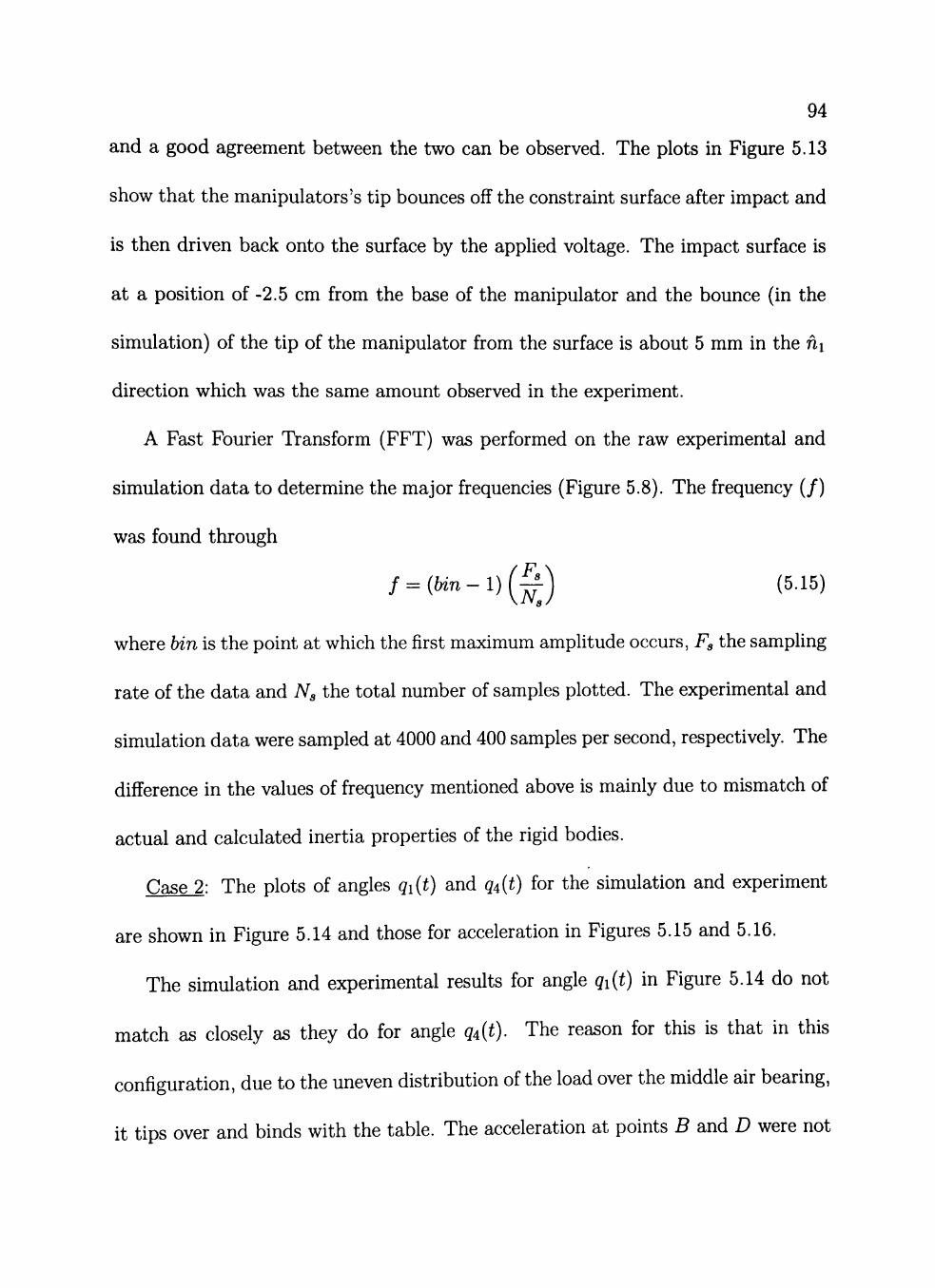
94

and a good agreement between the two can be observed. The plots in Figure 5.13

show that the manipulators's tip bounces off the constraint surface after impact and

is then driven back onto the surface by the applied voltage. The impact surface is

at a position of -2.5 cm from the base of the manipulator and the bounce (in the

simulation) of the tip of the manipulator from the surface is about 5 mm in the ni

direction which was the same amount observed in the experiment.

A Fast Fourier Transform (FFT) was performed on the raw experimental and

simulation data to determine the major frequencies (Figure 5.8). The frequency (/)

was found through

/ = ( 6 J n - l ) ( ^ ) (5.15)

where bin is the point at which the first maximum amplitude occurs, F^ the sampling

rate of the data and N^ the total number of samples plotted. The experimental and

simulation data were sampled at 4000 and 400 samples per second, respectively. The

difference in the values of frequency mentioned above is mainly due to mismatch of

actual and calculated inertia properties of the rigid bodies.

Case 2: The plots of angles qi{t) and 54(í) for the simulation and experiment

are shown in Figure 5.14 and those for acceleration in Figures 5.15 and 5.16.

The simulation and experimental results for angle qi{t) in Figure 5.14 do not

match as closely as they do for angle q^^t). The reason for this is that in this

configuration, due to the uneven distribution of the load over the middle air bearing,

it tips over and binds with the table. The acceleration at points B and D were not

95

compared since the experimental data was extremely noisy and filtering resulted in

a flat line that showed none of the expected trends.

As in Case 1, the major trends, the overall waveform and overall frequency, in

the experimental and simulation results are very close to each other. The FFT of

the acceleration data for this case is presented in Figure 5.17. The frequency of

the raw acceleration data from the experiment was calculated and varies between

9.31 and 9.71 Hz and that of the simulation between 10.05 and 10.14 Hz. These

frequencies were calculated via Eq. 5.15. In this case also, the experimental and

simulation data were sampled at 4000 and 400 samples per second, respectively.

The difference in time of impact in the experiment and simulation is once again

attributed to the reason discussed in Case 1 above. The difference in the frequencies

of the experimental and simulation acceleration data is also due to the variations

in inertia properties of the rigid bodies.

The FFT of the acceleration of the experimental data also showed the presence

of some higher frequencies and had a larger magnitude. This suggests that a large

portion of the energy is in the higher, possibly sonic, modes.

Case 3: In order to demonstrate the influence of backlash on the model, a square

of amplitude 0.5 V and frequency 0.667 Hz was applied to the base motor and a

)Itage 180° out of phase to that going to the base motor was applied to the middle

motor of the experimental setup and the resulting encoder and accelerometer values

were recorded. A similar signal was applied to the motors in the simulation and the

wave

vol

96

results were compared. The experimental and simulation results of the two angles

qi{t) and q^^t) are plotted in Figure 5.23. The amplitudes of the angles are very

close to each other and the frequency of the experimental and theoretical curves are

identical.

The experimental curves of the two angles (Figure 5.23) tend to deviate from

an equilibrium oscillating point. This is not the case in the simulation results. The

reason for the testbed results to deviate is friction between the air bearing and the

table. Theoretically, even with backlash, the beams should oscillate about a certain

point. But friction between the table and the air bearing prevents the beam from

returning to its original position and so in time, the beam tends to move away from

its original position.

In the model, the above mentioned friction is not included as this friction is

random, i.e. it is present only at certain high points on the surface of the table.

Nevertheless, both the simulation and testbed results exhibit the effect of backlash

as a flat region at the peak and trough of the waveforms in Figure 5.23.

Another point to note in the plot is that there is a phase lag between the ex-

perimental and simulation curves. When looked at closely, at time = 0, both the

experimental curves show a dead band indicating that there was backlash at the

start of the motion. But in the simulation, it was assumed that there was no initial

backlash at the start of the motion. This is evident through the initial (near) linear

rise of the angles at the start.

97

5.6.2 Comparison of Flexible and Rigid Body Models

The comparison of the rigid and flexible model is made via the two cases men-

tioned above and the results are presented in Figures 5.18 through 5.22.

Coordinates qi{t) and qs{t) of the rigid manipulator correspond to coordinates

qi{t) and q^^t) of the flexible manipulator. Figure 5.18 shows that the angles qi{t)

through 54 (í) of the rigid body model change abruptly on impact. The reason for

this is as follows. In the case of the flexible members, the energy on impact goes

into deforming the beam and also, some of the energy is dissipated by the damping

present in the beam. But in the case of the rigid manipulator, as the energy on

impact cannot deform the rigid beams, it goes into deforming the spring. In effect,

since the motion is abruptly stopped on impact, the kinetic energy is converted into

potential energy in the spring.

The plot of the tip of the manipulator in the ni direction (Figure 5.24) in both

Case 1 and Case 2 show that the overall motion of the rigid manipulator remains,

for the most part, identical to that of the flexible manipulator. But due to the

assumption that the beam is rigid in the latter case, there is a difference in time

the manipulator reaches the impact surface. AIso seen in Figure 5.24 is the tip of

the manipulators bouncing of the impact surface and returning back.

In the plots (Figures 5.19 through 5.22) that compare accelerations of the flexible

and rigid manipulators at various points (mentioned earlier) along the manipula-

tor, the rigid model's results exhibit only the overall waveform and not the higher

98

frequency waveforms. AIso, the acceleration at the instant of impact is higher than

that of the flexible model because, in the flexible model, some of the energy goes

into creating the higher frequency waves. The flrst beam and the second rigid body

(in the rigid model) have the same angular velocity and acceleration (as they are

governed by the same coordinate frame) but the distance of point B is almost twice

the distance of point A from the Newtonian frame, the acceleration on impact at

point B has a higher value.

5.6.3 Control of the Flexible Manipulator

A very simple proportional control law* was used to control the motion of the

manipulator in order to demonstrate the usefulness of the simulation tool. The

applied control law was

Ti{t) = -dampi * 5 - springi{qi{t) - cQi), (5.16)

where T is the torque required to drive the beam i to a desired position, dampi is

the damping applied to lessen overshoot, spring^ provides the driving torque, q^ the

angle at time t and cQi the commanded angle or the desired final angular orienta-

tion of beam i. After calculating the required torque (T^), the voltage required to

generate that torque was calculated via

V, = ^-KtiniSi. (5.17) rii Kti

^The control law was implemented only in the simulation.

99

The terms used in Eq. 5.17 are as explained in Section 5.3.1.

A variation of the above control law was to command the tip of the manipulator

to go to a fixed point in its workspace. In this case, an inverse kinematic routine

(using the Newton-Raphson [70] technique) was used to calculate the angular orien-

tations qi{t) and q^^t) of the beams for the tip to reach the desired position. Using

these values of qi{t) and q^^t) as the two commanded angles {cQi), Eq. 5.16 was

used to drive the manipulator to the desired position.

A result of application of the above control law is shown in Figure 5.25. Shown

in the figure is the path traced by the tip of the manipulator (in the {x, y) Cartesian

frame) and the plots of angles qi{t) and q^^t). For this case, the manipulator was

initially positioned such that its tip was at point (1.15,1.2)^ and a final position of

(1.0, 1.0) was specified (which is in the workspace of the manipulator). The straight

line in the plot of angles indicates that steady state has been reached.

In order to further demonstrate the model's use in control applications, a sanding

like operation was simulated where the tip of the manipulator was forced to move

along the constraint surface by varying the commanded position of the tip in time.

The control law discussed above was used in this case also.

It is interesting to note from Figures 5.26, 5.27 and 5.28 that the manipulator

realizes the full motion regime. Figure 5.26 shows the position of the tip of the

^The coordinates of each point specifier the x and y distances, in meters, w.r.t. the Newtonian frame of reference.

100

manipulator in the ni or x-direction, Figure 5.27 shows the position of the tip of

the manipulator in the n^ or î/-direction and Figure 5.28 the plot oî x ws y position

of the tip of the manipulator.

The constraint surface is 25 mm in the negative ni direction. The above plots

show the time and position at which the tip leaves the surface. In the close up view

of the tip position in the í/-direction, the wavy nature of the curve shows the effect

impact has on the motion of the flexible manipulator. Another effect of impact

with friction that the model was able to predict direction reversal. This effect is

well noticed in the animation but can also be noticed in the plot of the tip position

in the x-direction at time í = 2.25 seconds.

101

do while(t . le. tf)

call torque_paraineters(count, ybacklash)

check to see If contact is made

duitimyl = tip_position(t, y, Ll, L2)

if (dummyl .le. (h + 0.005)) then

delt = deltnear skip = skipnear

else delt = deltfar skip = skipfar

end if

if(const.eq.0)then if(duinmyl . le. -h) then

const=l call momentum(y)

arm LSODA for a new problem in constrained coords write(75, 250)t, acc(l), acc(2), acc(3), acc(4) istate=l

endif endif

time = t

if(const.eq.0)then call YtoX(n,x,y)

tout=t+delt call lsoda(eom,n,x,t,tout,itol,rtol,atol,itask,istate,iopt,

í rwork,lrw,iwork,liw,JACOB,jt) call Xtoy(n,x,y)

else if(swsignold.eq.O)swsignold = switch(y, nc, t) call YtoXc(nc,xc, y) tout = t + delt tipvel_n2 = tip_velocity(t, y, Ll, L2) call lsoda(eomcfriction,nc,xc,t,tout,itol,rtol,atol, itask,

í istate,iopt,rwork,lrw,iwork,liw,JACOB,jt) call XctoY(nc,xc,y) call update(y)

swsign = switch(y, nc, tout) call print_swsign(swsign, swsignold) if(swsign*swsignold .gt. 0)then swsignold = swsign else const=0 swsignold=0 arm LSODA for a new unconstrained problem istate=l endif

endif

call print(t, tf, y, count, Ll, L2)

end do

Figure 5.1: The Logic

102

Base Motor & Gearbox Middle Motor & Gearbox

Acceleromerters

Beams

Air Bearings

Figure 5.2: Experimental Setup

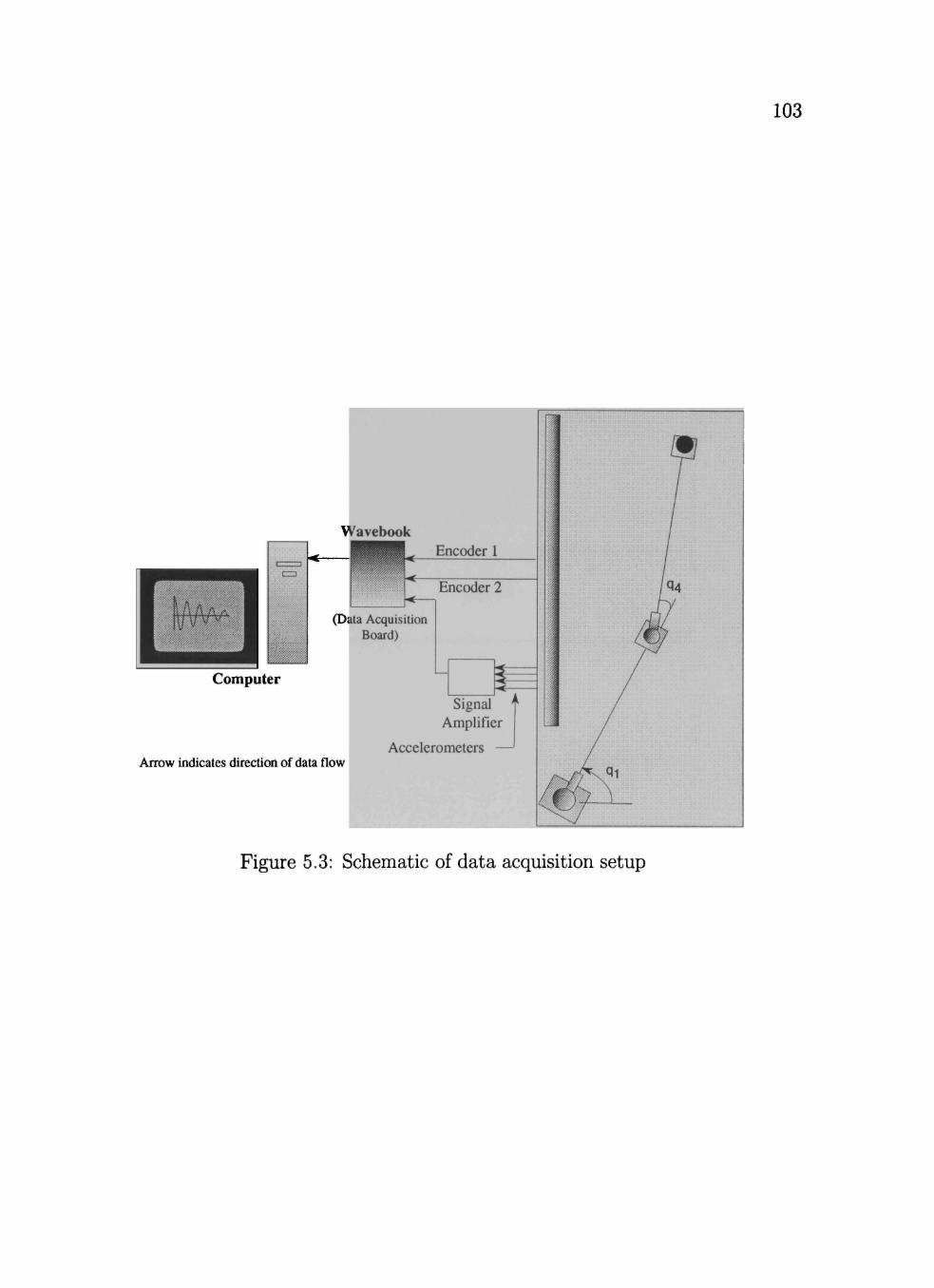
103

Computer

Wavebook Encoder 1

Encoder 2

(Data Acquisition Board)

Signal Amplifier

Accelerometers Arrow indicates direction of data flow

Figure 5.3: Schematic of data acquisition setup

104

c

a>

1 0 n

20-

10-

0-

10-

20-

•30-

40- 1

1

1 i ! 1 <

Experíment

,i : —ll lP^vvv^

i i

0 2 Tlme (sec)

c .2

<o o o <

'xn -,

20-

10-

fí -u

10-

20-

JU

40 -

/ • -

1 1 1 1 > 1

Simulation

mim~~

1 • í '

0 2 Time (sec)

Figure 5.4: Case 1 : Plots of acceleration of mid-point of first beam

105

.2

i

" n -1 jyj

20-

10-

0-

10-

20-

30-

40-

. , ^ - ^ . - .

1 1 1 < 1 1 '

Experíment

1 1

0 2 Time (soc)

(0

9

I

i n ^ j\j

20-

10-

n -U

-10-

-20-

-30-

-40- 1 1 — • 1 1 1 1 ' 1 1

(11/11 | V U

Simulation

W/w^

1 '

V/>^,''>w>»^v^

1

0 2 Time (sec)

Figure 5.5: Case 1 : Plots of acceleration of second rigid body

106

CM

C .S 9

30

20 -

10 -

0

- 1 0 -

-20 -

-30

-40 0 2

Time (sec)

Experíment

Simulation

CM

i c .2 1 a>

Figure 5.6: Case 1 : Plots of acceleration of mid-point of second beam

107

Experíment

CM

&

a>

8 <

Simulatlon

CVJ

<"

c .2 '? _2 <D

8 <

Figure 5.7: Case 1 : Plots of acceleration of fourth rigid body

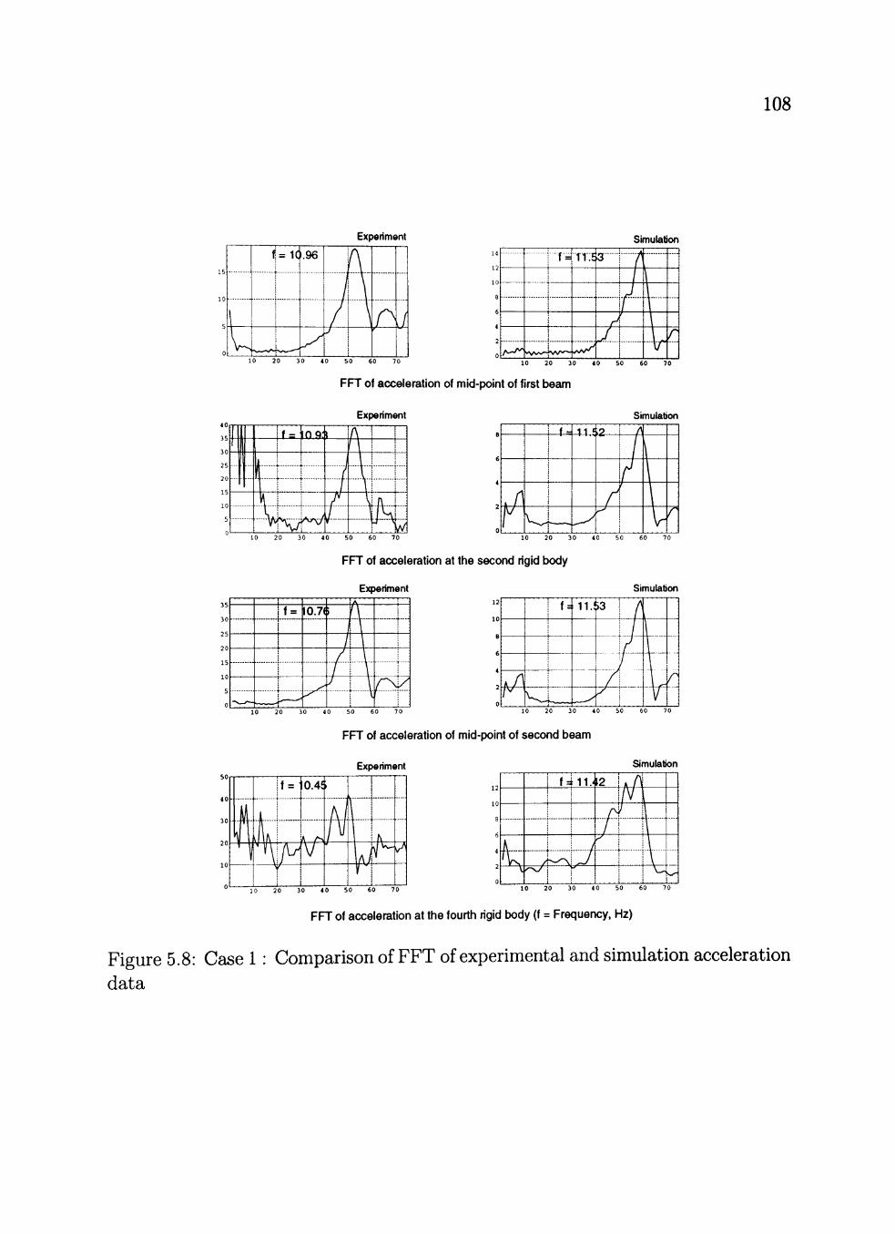
108

Experíment Simulation

í=1(

1 1

1

.96

A/ 10 20 30 40 50 60 70

rr= 1 1

i i 1

ii.i . 3 j 'A

'ff^"— i/

i^ /í 4-

• • • •

- •

10 20 30 40 50 60 70

FFT of acceleration of mid-point of first beam

Experíment Simulation

1 lf=

—+—

+"--

H i V. i

inq; ' lA ! 1 \ !

1 !

\ i

\ [ A

\i~A

i f--

i f^ K i

111,9 i /\

\

V r 10 20 30 40 50 60 70 10 20 30 40 50 60 70

FFT of acceleration at the second rígid body

Experíment Simulation

1 if =

1

+

I0.7(

/' \ / ' 1

^

• • • • •

- » • - -

(\

1 f =

^ v u _

11.1

—

i3 /

•J.

y i 1

~\f^

...

10 20 30 40 50 60 70 10 20 30 40 50 60 70

FFT of acceleration of mid-point of second beam

Experíment SJmulation

\ ' !

- - • • ( • ' • •

i f = '

. i

11 i

0.4;

v/ í T i 1 1

. 1 H ....

f=t11..

\ T 1

1

Í2 1 . /1

/ i ....

10 20 30 40 50 60 70 10 20 30 40 50 60 70

FFT of acceleration at the fourth rigid body (f = Frequency. Hz)

Figure 5.8: Case 1 : Comparison of FFT of experimental and simulation acceleration data

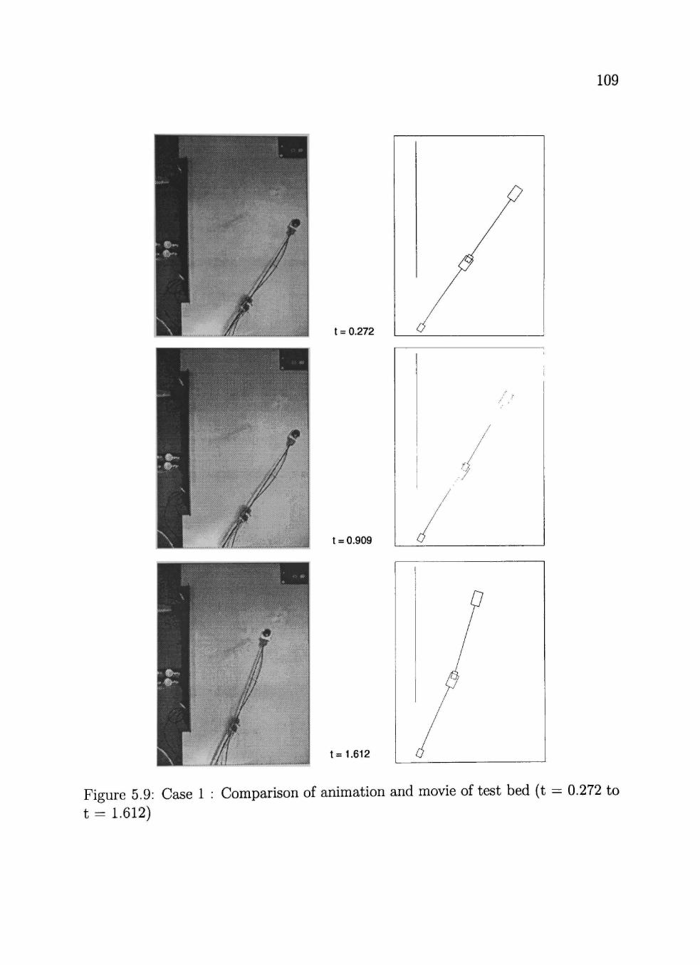
109

t = 0.272

t = 0.909

t = 1.612

Figure 5.9: Case 1 : Comparison of animation and movie of test bed (t = 0.272 to t= 1.612)

110

t = 2.100

t = 2.302

•

t = 2.818

Figure 5.10: Case 1 : Comparison of animation and movie of test bed (t = 2.100 to t = 2.818)

111

^SC^.^'ÍÍ k

t = 2.12

t = 2.34

t = 2.72

Figure 5.11: Case 1 : Comparison of animation and movie of test bed (t = 2.12 to t = 2.72) (Closeup View)

112

t = 2.81

t = 2.97

t = 3.44

Figure 5.12: Case 1 : Comparison of animation and movie of test bed (t = 2.81 to t = 3.44) (Closeup View)

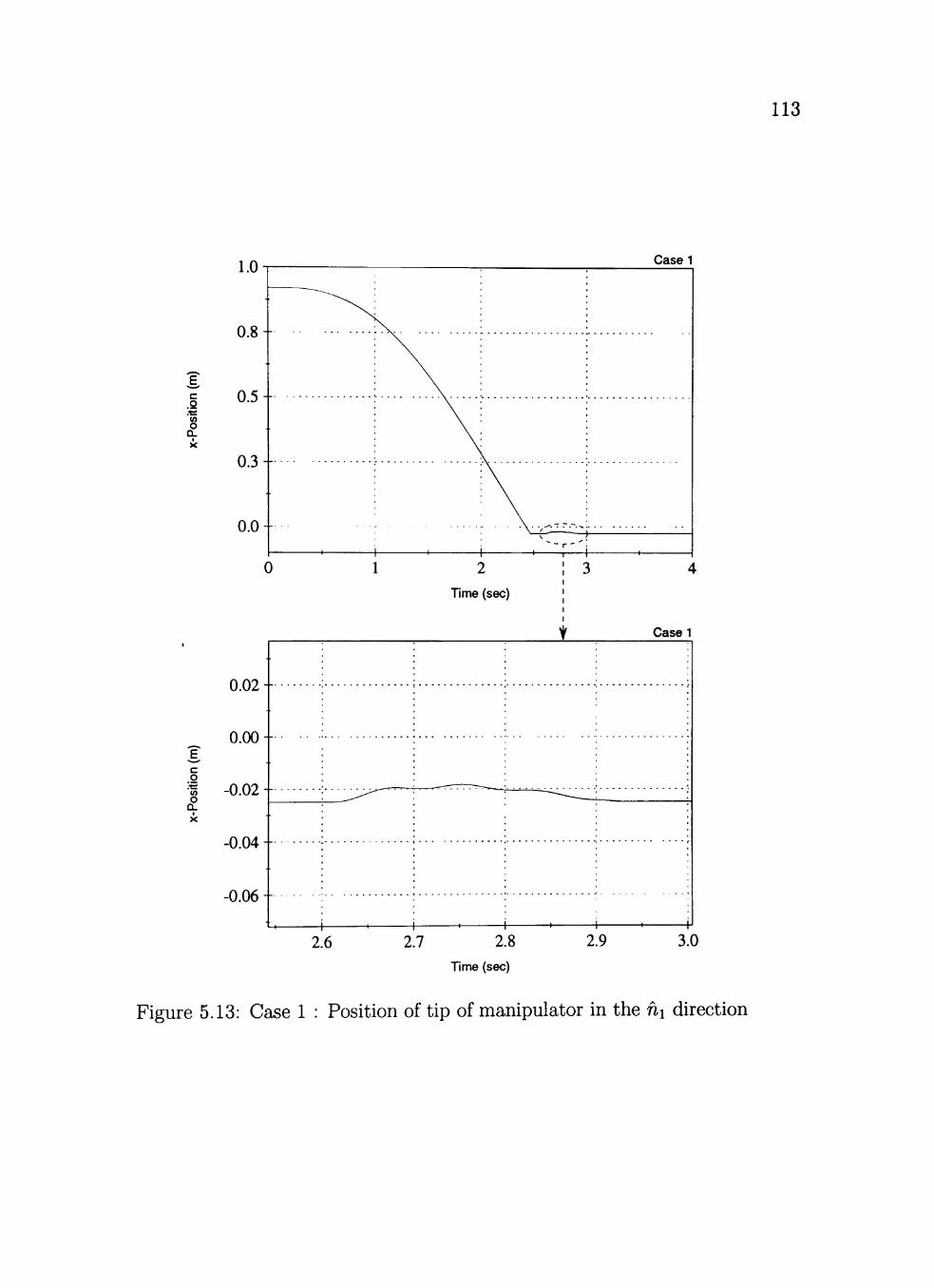
113

Case 1

c .S .tí

w> o Q .

C 2

! t ; U) O .

2.6 2.7 2.8

Time (sec)

0.02-

0.00-

-0.02 -

-0.04 -

-0.06 -

1

_ , ^ > ^

1 ' 1 1 < 1

y

• — _ _ _

1 — - ^ 1

Case 1

1 < i-

2.9 3.0

Figure 5.13: Case 1 : Position of tip of manipulator in the åi direction

114

c T3 «

O)

c <

1.6

1.4--

1.2 -

1.0-;

0.8 -

0.6 -

0 .4 -

0.2

0.0

-0.2

Case 1

-*- q.| Experimental

q^ Experimental

q.^ Slmulation

q Simulation

.,.»-'

0 2 Time (sec)

c ca

TJ

_2 C3>

c <

1.6 f w w . w w s / s ^ s / ^ / v x / N ^ v y y v X X X X X y ^ ,

1.4 -

1.2-

1.0 -

0.8 -

0.6 -

0 .4 -

0.2 -

0.0

Case2

^ • H > -

+-<- -(-+ -H- -H- -H-^

- H -H- +^ .<>-^

0 1 2 Time (sec)

" q.| Exper iment

••• q ^ Exper iment

q.| Simulation

q ^ Simulat ion

.-H-t-*- -H- -H--

Figure 5.14: Plots of angles qi and q^

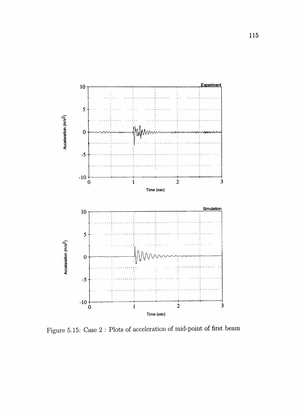
115

CM <"

. 2 a> o

CM

C

.2 & _o <D U

10

5 -

0

- 5 -

•10

-~—j w • [

Exoeríment

^.,^„-,.1—„p^

' ' ' '

; i , i 1

0

10

5 -

0

- 5 -

-10 0

Time (sec)

Simulation

Time (sec)

Figure 5.15: Case 2 : Plots of acceleration of mid-point of first beam

116

CM

{0

_2 <D

o

lOn

5-

0-

-5-

10-

^ ^ ^

, j

W-MM..^-/>., »y||VWANr/S.

1 1

^•Vr^^"v*''^-»>'>V'^^

' 1

gw'-'^g ...•••^M.^aN.^/'WVV

1 '

Exoeríment

*N<-wSíWwVvWVwA

0 1 2 Time (sec)

CM

c .2 2 _æ (D

o

10

5 -

- 5 -

-10 0

Time (sec)

Simulation

Figure 5.16: Case 2 : Plots of acceleration of mid-point of second beam

117

Experiment Simulation

10 20 30 40 50 60 70

0.5

0

f = io.i;> ...L...|.

1 i \ 1 \ i

j N ^

i

....

10 20 30 40 50 60 70

FFT of acceleration of mid-point of first beam

Experiment Simulaticxi

10 20 30 40 50 60 70 10 20 30 40 50 60 70

FFT of acceleration at the second rigid body

Experíment Simulation

0 !

f = í .31

i \ /

1

i V

1.25

1

0 . 7 5

0 .5

0 . 2 5

0

[ !

-A í 1 1 -1

\- i —

• ^

10.1 4

- / _...L.

• • "

10 20 30 40 50 60 70 10 20 30 40 50 60 70

FFT of acceleration of mid-point of second beam

Experíment Simulation

f = lO.Oi i

....

10 20 30 40 50 60 70 10 20 30 40 50 60 70

FFT of acceleration at the fourth rigid body (f = Frequency, Hz)

Figure 5.17: Case 2 : Comparison of FFT of experimental and simulation accelera-tion data

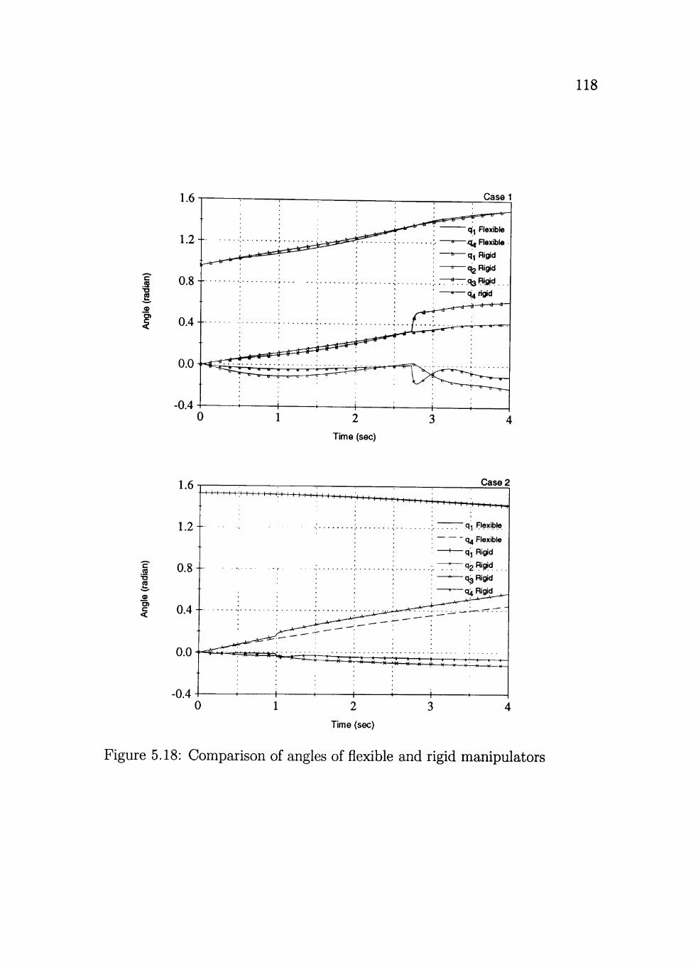
118

Case 1

c .S •o 2, <D

Case2

c

S, _2 o>

Figure 5.18: Comparison of angles of flexible and rigid manipulators

119

CM JO

c .2 2 (D

" n z.\j

15:

10:

5:

0-

-5-

-10:

-IS-

r

1 1 ' 1 1 <

(1 1

1

1 >

1 . . . . .^

1

Case 1

Flexipie Moaei

" ^ Rigid Model

j

• -i '

fAhA^

1

0 2

Time (sec)

Case2

CM

c 2 •? _« (D

8 <

0

-5 0 2

Time (sec)

- ^ o ^ y ^ ^ s , ^ ^

1

1,

> 1 1 1

11* l/Vww-

F l e x o e M U U U I -Rigid M

1 1 1 i '

txiel

1

Figure 5.19: Comparison of acceleration of mid-point of first beam of flexible and rigid manipulators

120

CM J>>

C

.2 1 _2 (D u o <

20 n

15:

10-

5-

0-

-5-

•10-

15^ ' 1 1 ' 1 1 1 1

1

'i

i tl

1

Case 1

Rexipie Mooei

- ^ Rigi<i Mo<Jel

ir

- i 1

V ^ A A ^

1

0 2

Time (sec)

Case2

CM

c o 1 (D

0

0 2

Time (sec)

- n ^ ^ ' S í ^

1

l

:

1 h

/ ih

m

1

fi^

1 1

\f\j\N^

1 <

Flexible Mooei T -Rigid M

i '

3del

1

Figure 5.20: Comparison of acceleration of second rigid body of flexible and rigid manipulators

121

Case 1

CM j "

2 .æ

Case2

CM </>

2 . 2 8

Figure 5.21: Comparison of acceleration of mid-point of second beam of flexible and rigid manipulators

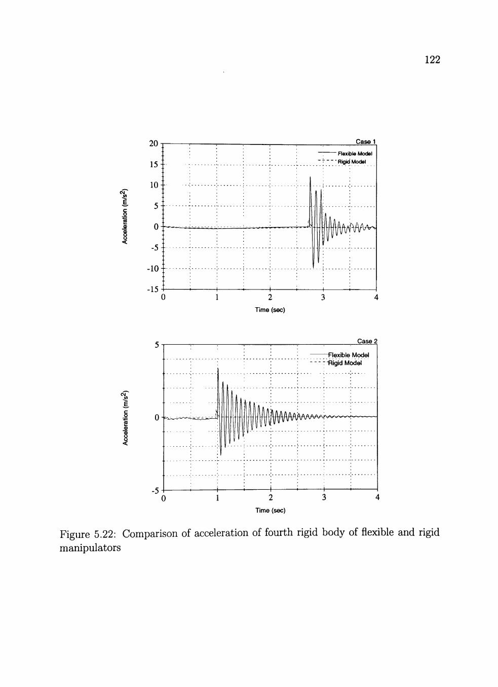
122

CM <0

C

.2 2 .S

'>0 n

15:

10-

5-

0:

-5;

-10:

- 1 5 - 1 1 ' 1 1 1

^

Case 1

-

1 1 1

)-iexipie iv xiei Rigid Model

j||lftft/MA^

1 >

0 2 Time (sec)

Case2

CM

<"

c .2 1 .2 <D

I

0

0 2

Time (sec)

1

1 s

i h

.

III. II |||H

i 1

Flexible Mcxiei " -Rigid Model

1 i i ' p

Figure 5.22: Comparison of acceleration of fourth rigid body of flexible and rigid manipulators

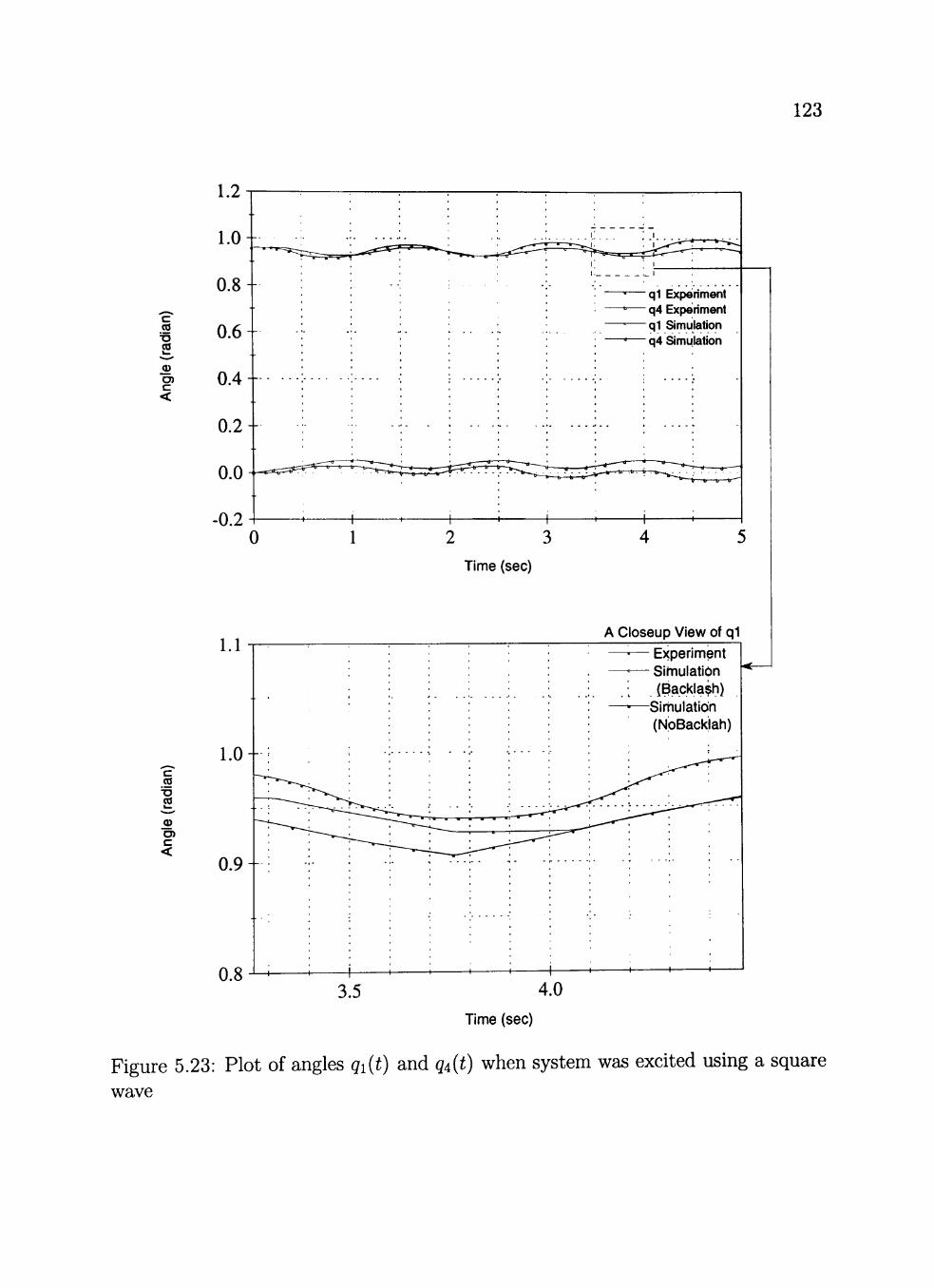
123

c (0

_© O) c <

c cg

CO

O) c <

q1 Expeiriment q4 Experiment

-q1 Simulation q4 Simulation

^—b b — b - ~-t—1»—~b—•V

A Closeup Vlew of q1

Time (sec)

Figure 5.23: Plot of angles qi{t) and q^^t) when system was excited using a square wave

124

T3

? (S

•c 3 (0

â E i e (D

B <a

b

1 n ^ l . U

0.9-

0.8-

0.7-

0.6-

0.5-

0.4-

0.3-

0.2-

0.1-

0.0-

-n 1 -

1 1 + ^ r ^

+.> -+ \ + \

+ \ +• \ '

' i

+ \ - 1 - \

-í-\ - t - \

+

4 \

\ ^

' i < 1

Case 1

risxime + Rigidl

1 < 0 2

Time (sec)

Case2

(D O (0

"C 3

co 13 (Q Q.

E E S

c <a

'Ô

Fiexible + Rígid

Time (sec)

Figure 5.24: Comparison of tip position {ûi direction) of rigid and flexible manip-ulators for Casel and Case 2

125

Plot of Tip Position

a>

c

o

0.9 1.0 x-Coordinate (m)

c (0

•v 2, _2

I

0 10 20 Time (sec)

1 T -, l .Z

1.0-

0.8-

0.6-

0.4-

0.2-

0.0-

0 ? -

/ \ /

/ \ / \ /

• • • /

• /

/ / /

j

/

1 1

/

1 X i (

Plot of Angles

i 1

Angle q^

"Angleq^

1 30

Figure 5.25: Demonstration of Control - Plot of tip position and angles of flexible manipulator (Position control)

c <S

• •a

2, _2 c <

1.8

1.6

1.4

1.2

\ • \ /

\ / \ /

+ x /••

1.0 -

0.8 -

0.6

\ / \ /

0

Plot of angles

\ / \ /

/

-> 1 -

/

\ - . V

/ /

\ / \ / \ /

\ / \ / •\ /• \ / \ /

. . . \ ; . . .

Time (sec)

\ / \ / \ / \ / \ / \ /

qi

^2

8 10

126

0.16 Plot of x-Position

8 c .2

Q. X

Figure 5.26: Demonstration of Control - Plot of x-position of tip and angles of flexible manipulator (Sanding operation)

127

c .S

.

c .2

<n o Q.

Time (sec)

Figure 5.27: Demonstration of Control - Plot of y-position of tip of flexible manip-ulator (Sanding operation)

128

1.35

c .S . t : <0 o a.

c .2 w o

1.00 -0.0300 -0.0275 -0.0250

x-Position (m)

-0.0225 -0.0200

Figure 5.28: Demonstration of Control - Plot of xy-position of tip of flexible ma-nipulator (Sanding operation)

CHAPTER VI

SUMMARY AND FUTURE DIRECTIONS

6.1 Summary

The work presented in this dissertation has three main contributions as stated

in the objectives.

The flrst main contribution of this dissertation was the development of a non-

linear, high fldelity hybrid model using the hybrid parameter multiple body method

[4, 5, 9, 11]. To overcome the drawbacks of other models discussed in the Hterature

review, this model included

1. Complete motion regime comprising

a. Free motion of the manipulator

b. Contact/Impact with a workpiece or environment

c. Post-impact constrained motion

2. Dynamics of all interconnecting rigid bodies,

3. Dynamics of all driving motors,

4. Dynamics and backlash of the gearboxes, and

5. Friction in the constrained mode of motion.

The second contribution of this work was the successful verification of the above

model using a two-Iink flexible manipulator described in Section 5.5. This is evident

from the results presented in Figures 5.4 through 5.16. The discrepancies in the

129

130

results from the testbed and the simulation were mainly due to the assumption that

the points of connection between the different bodies in the test setup were with

no clearance. Another source of error was in estimation of the parameters of the

gearbox and rigid bodies.

The third main contribution was the comparison of the high-fldelity model to

the lower fidelity model. In the low-fidelity model, the elasticity of the beam was

modeled as a torsional spring and the beams were considered to be rigid bodies.

Although, the simplification is made with respect to the elastic member, the rigor

of the model was maintained by including the complete motion regime, dynamics

of motors and gearboxes and friction in the constrained mode of motion. The

comparison of this model was made to see if the lower-fidelity model will be suitable

for control applications. But as seen from the plots of the angles, tip position and

accelerations, the rigid body model does not pick up the complete dynamics during

the impact phase. AIso, when accurate positioning is required, the rigid body model

will not be well suited for control applications.

Other significant contributions are

1. The process of impact is not modeled using a coefficient of restitution. Hur-

muzlu [63] has shown that the value of coefficient of restitution varies with

the angle of impact. Hence using a constant coefficient of restitution is bound

to introduce errors. But in the approach utilized in this research, the un-

certainty that arises as a result of using a constant value of the restitution

131

coeflíicient is eliminated by modeling the impact process as an instantly applied

non-holonomic constraint. The experiment data confirms this.

2. Although the number of modes of vibration used to describe the shape of the

beam was two, the model manifested most of the dynamic characteristics of

the test setup.

3. The rigid body model was able to predict the overall motion of the manipulator

with reasonable accuracy in the free flight mode.

4. Another point of interest to note is that the full flexible model has only six

degrees of freedom and the rigid body model has four degrees of freedom.

This shows that with a minimum number of modes most of the vibratory

characteristics of the test manipulator were picked up by the model. Hence,

by using lower number of modes and the explicit minimal equations of motion,

the terms of the inertia matrix of the equations of motion will be relatively

smaller and computationally efficient and this is amenable to control design

usage.

5. In the last section of Chapter V a very simple control law was implemented

and was shown that the model is suitable for control appHcations. As a note

on the time taken to run a simulation, it took a 40 second simulation, that

involved the control law, less than 10 seconds to run on a DEC Alpha UNIX

server.

132

Finally, reiterating, a model to predict the dynamics of a flexible manipulator

over the full motion regime was developed and was verifled successfully with a

planar two-Iink flexible manipulator. A low-fidelity rigid body model of the flexible

manipulator was also developed and its dynamics were compared with that of the

high-fidelity full flexible model to see if the low fldelity model well suited for control

applications. Thus the three main objectives stated in Chapter II have been met.

6.2 Future Directions

The research discussed in this dissertation can be extended in various directions

mentioned below.

1. Verification of a three-dimensional model.

2. This work was limited to the case of single point contact. Future work can ex-

tend the scope of this dissertation to verification of problems involving multiple

point contact.

3. One other extension (though in a smaller scale) would be to include members

that translate, in the model.

4. The code could be modified to check for stiction at the instant of impact and

also during constrained motion.

5. A natural extension of the rigid body model would be to break the beam into

two or more parts, each connected together with torsional springs, and see if

the resulting model better approximates the full flexible model. However, this

133

model would have the same degrees of freedom as the full flexible two-mode

model, and probably would not pick up the flexible modes well.

6. The developed model deals with impact with a rigid, non-deformable surface.

Impact with structures that deform (but not permanently) can be studied.

7. Develop a controller to control the motion of the manipulator throughout the

entire motion regime.

REFERENCES

[1] ABAQUS. Habbitt, Karlsson k Sorensen, Inc, Pawtucket, RI.

[2] Mathematica. Champaign, IL, USA.

[3] ProEngineer. Michigan, USA.

[4] A. A. Barhorst. On Modeling the Dynamics of Hybrid Parameter Multiple Body Mechanical Systems. PhD thesis, Texas kkM University, CoIIege Station, Texas, 1991.

[5] A. A. Barhorst. Closed form modeling of continuous parameter robotic systems-contact/impact and wave propagation. American Society of Mechanical Engi-neers, Design Engineering Division (Publication) DE, 57:39-47, 1993.

[6] A. A. Barhorst. Systematic closed form modeling of hybrid parameter multiple body systems. In Proceedings of the ASME Winter Annual Meeting, Paper # 93-WA/DSC-l, New Orleans, Louisiana, November 1993.

[7] A. A. Barhorst. Contact/impact in hybrid parameter multiple body mechanical systems-extensions for higher order continuum models. Transactions ofASME, 120:142-144, March 1998.

[8] A. A. Barhorst. On modeling variable structure dynamics of hybrid parameter multiple body systems. Joumal of Sound and Vibration, 209(4):571-592, 1998.

[9] A. A. Barhorst and L, J. Everett. A methodology for modeling hybrid param-eter multiple body systems. In Proceedings of the ASME Symposium on Dy-namics of Flexible Multibody Systems: Theory and Experiment, pages 197-205, Anaheim, CA, November 1992.

[10] A. A. Barhorst and L. J. Everett. Obtaining the minimal set of hybrid param-eter differential equations for mechanisms. In Proceedings of the ASME Design Engineering Technical Conference, DE-Vol. 4Z pages 311-316, Phoenix, AZ, September 1992.

[11] A. A. Barhorst and L. J Everett. Contact/impact in hybrid parameter multiple body mechanical systems. Joumal of Dynamic Systems, Measurement and Control, 117(4):559-569, 1993.

[12] A. A. Barhorst and L. J. Everett. Contact/impact in hybrid parameter multiple body systems. In Proceedings of the ASME 16th Annual Energy-Sources Tech-nology Conference & Exhibition, Dynamics and Vibrations Symposium, pages 27-35, Houston, TX, January 1995.

[13] A. A. Barhorst and L. J. Everett. ModeUng hybrid parameter multiple body systems: A different approach. The Intemational Joumal of Nonlinear Me-chanics, 30(1):1-21, 1995.

[14] A.A. Barhorst. Symbolic equation processing utilizing vector/dyad notation. Joumal ofSound and Vibration, 208(5):823-839, 1997.

134

135

15] V. Bhatt and J. Koechling. Partitioning the parameter space according to different behaviours during three-dimensional impacts. Transactions of the ASME, 62:740-746, September 1995.

16] V. Bhatt and J. Koechling. Three-dimensional frictional rigid body impact. Joumal of Applied Mechanics, 62:893-898, December 1995.

17] R. M. Brach. Rigid body collisions. Joumal of Applied Mechanics, b6:133-13S, March 1989.

18] R. M. Brach. Classical planar impact theory and the tip impact of a slender rod. Intemational Joumal of Impact Engineering, 13(l):21-33, 1993.

19] N. J. Carpenter, R. L. Taylor, and M. G. Katona. Lagrange constraints for transient finite element surface contact. Intemational Joumal for Numerical Methods in Engineering, 32:103-128, 1991.

20] C. W. Chang and A. A. Shabana. Spatial dynamics of deformable multibody systems with variable kinematic structure: Part 1-dynamic model. Joumal of Mechanical Design, 112:153-159, June 1990.

21] C. W. Chang and A. A. Shabana. Spatial dynamics of deformable multibody systems with variable kinematic structure: Part 2-dynamic model. Joumal of Mechanical Design, 112:160-167, June 1990.

22] J.J. D'Azzo and C.H. Houpis. Linear control system analysis and design. Mc-Graw HiII Book Company, New York, 2nd edition, 1981.

23] S. Dubowsky. On predicting the dynamic effects of clearances in planar mech-anisms. Joumal of Engineering for Industry, pages 317-323, February 1974.

24] S Garza. Theoretical and experimental investigation of the dynamics and bifur-cations of an impacting spherical pendulum with large deflection. PhD thesis, Texas Tech University, Lubbock, TX, 1993.

25] S. Garza and A. Ertas. Experimental investigation of the dynamics and bi-furcations of an impacting spherical pendulum. In 1995 Design Engineering Technical Conference, volume 3 - Part A of DE-VoL 84-1, pages 181 - 189. ASME, 1995.

26] W. Gau and A. A. Shabana. Use of the generalized impulse momentum equa-tions in analysis of wave propagation. Joumal of Vibration and Acoustics, 113:532-542, October 1991.

27] W. Gau and A. A. Shabana. Effect of finite rotation on the propagation of elastic waves in constrained mechanical systems. Joumal of Mechanical Design, 114:384-393, September 1992.

28] W. Gau and A. A. Shabana. Use of the finite element method in the analysis of impact-induced longitudinal waves in constrained elastic systems. Joumal ofMechanical Design, 117:336-342, June 1995.

136

[29] B. P. Gautham and N. Ganesan. Finite element analysis of contact-impact be-tween a shell of revolution and a rigid wall. Intemational Joumalfor Numerical Methods in Engineering, 37:3215-3262, 1994.

[30] Inwan Han and B. J. Gilmore. Multi-body impact motion with friction-analysis, simulation, and experimental validation. Transactions of the ASME, 115:412-422, 1993.

[31] I. Hunek. On a penalty formulation for contact-impact problems. Computers and Stmctures, 48:193-203, 1993.

[32] Y. Hurmuzulu and D. B. Marghitu. CoIIisions of planar kinematic chains with multiple contact points. Advances in Robotics, Mechatronics and Haptic Inter-faces, 49:271-280, 1993.

[33] R.L. Huston. Multibody Dynamics. Butterworth-Heinemann, Ist edition, 1990.

[34] K.L. Johnson. Contact Mechanics. Cambridge University Press, 1985.

[35] Ahmet Kahraman. On the response of a preloaded mechanical oscillator with a cIearence:period-doubIing and chaos. Nonlinear Dynamics, 3:183-198, 1992.

[36] T. R. Kane, R. R. Ryan, and A. K. Banerjee. Dynamics of a cantilever beam attached to a moving base. Joumal of Guidance, 10 (2):139-151, 1987.

[37] T.R. Kane and D.A. Levinson. Dynamics : Theory and Application. McGraw HiII Series in Mechanical Engineering. McGraw HiII, New York, 1985.

[38] H. Kazerooni, T. Sheridan, and P. Houpt. Roboust compHant motion for ma-nipulators, part 1: The fundamental concepts of compliant motion. lEEE Joumal of Robotics and Automation, RA(2) No. 2:83-92, 1986.

[39] L. M. Keer and J. C. Lee. Dynamic impact of an elastically supported beam-large area contact. Intemational Joumal of Engineering Science, 23(10):987-997, 1985.

[40] L. M. Keer and J. C. Lee. Dynamic impact of an elastically supported beam-large area contact. Intemational Joumal of Engineering Science, 23 (10):987-997, 1985.

[41] J. B. Keller. Impact with friction. Joumal of Applied Mechanics, 53(l):l-4, March 1986.

[42] Y. A. Khuleif and A. A. Shabana. Dynamic analysis of constrained system of rigid and flexible bodies with intermittent motion. Joumal of Mechanisms, Transmissions and Automation in Design, 108:38-45, March 1986.

[43] Y. A. Khulief and A. A. Shabana. Impact responses of multi-body systems with consistent and lumped masses. Joumal of Sound and Vibration, 104(2): 187-207, 1986.

137

44] Y. A. Khulief and A. A. Shabana. A continuous force model for the impact analysis of flexible multibody systems. Mech. Mach. Theory, 22(3):213-224, 1987.

45] R.M. Kloecker. Analysis and simulation of the combined effects of non-Iinear friction and gear backlash on an electromechanical position control system. Master's thesis, Michigan Technological University, 1992.

46] S. H. Ko and B. M. Kwak. Frictional dynamic contact analysis in deformable multibody systems. Finite Elements in Analysis and Design, 12:27-34, 1992.

47] Y. W. Kwon and E. S. McDonald. Optimization technique for contact stress analysis with application to low velocity impact to composite beams. Materials and Design Technology, PD-voI. 62:151-163, 1994.

48] H. M. Lankarani and P. E. Nikravesh. A contact force model with hystere-sis damping for impact analysis of multibody systems. In ASME-DE Series, Volume 19, Paper no. 89-doc-89, pages 45-51, Montreal, Quebec, Canada, September 1989.

49] H. M. Lankarani and P. E. Nikravesh. Hertz contact force model with perma-nent indentation in impact analysis of solids. Advances in Design Automation-Volume 2, DE, 44-2:391-395, 1992.

50] D. B Marghitu. Frictional impact of an elastic body. Design Engineering Technical Conferences, vol 3-PaH-A, DE-VoI. 84-1:191 -201, 1995.

51] D. B. Marghitu and Y. Hurmuzlu. Longitudinal impact of rectilinear elastic link in kinematic chains. Vibration ,Shock, Damage and Identification of Mechanical Systems, DE-VoI. 64:27-31, 1993.

52] K. Marudachalam and F. H. Bursal. Numerical study of an impact oscillator. 1995 Design Engineering Technical Confemces-Volume 3-Part A, DEi-VoI. 84-1:159-170, 1995.

53] J. K. MiIIs and C. V. Nguyen. Robotic manipulator collisions: ModeHing and simulation. Joumal of Dynamic Systems, Measurement and Control, 114:650-659, 1992.

54] D. Osmont. Computation of the dynamic response of structures with unilat-eral constraints (contact)-comparision with experimental results. Computer Methods in Applied Mechanics and Engineering, 34:847-859, 1982.

55] J. K. Park and B. M. Kwak. Three-dimensional frictional contact analysis using the homotopy method. Joumal of Applied Mechanics, 61:703-709, September 1994.

56] L. R. Petzold and A.C. Hindmarsh. Lsoda.. livermore solver for ordinary differ-ential equations, with automatic method switching for stiff and nonstiff prob-lems. Freeware, May 1982.

138

[57] F. Pfeiffer and C. Glocker. Impacts with friction. DE-Vol. 84-1, 1995 Design Engineering Technical Conferences, DE-VoI. 84-1:171-180, 1995.

[58] J.N. Reddy, editor. Energy and variational methods in applied mechanics. John Wiley and Sons, New York, 1984.

[59] M. W. Salveson and R. L. Taylor. An explict-implicit contact algorithm. Nu-merical Methods in Stmctural Mechanics, 204:99-122, 1995.

[60] W. P. Schonberg, L. M. Keer, and T. K. Woo. Low velocity impact of trans-versely isotropic beams. Intemational Joumal of Solids Stmctures, 19(4):871-896, 1987.

[61] C. W. Shao, F. W. Liou, and A. K. Patra. A contact phase model for the anal-ysis of flexible mechanisms under impact loading. Computers and Structures, 49(4):617-623, 1993.

[62] C. Sridhar and K. P. Rao. Estimation of low-velocity impact damage in lami-nated composite circular plates using non-Iinear finite element analysis. Com-puters and Stmctures, 54(6): 1183-1189, 1995.

[63] D. Stoianovici and Y. Hurmuzulu. A critical study of the aplicability of rigid-body collision theory. Joumal of Applied Mechanics, 63:307-316, June 1996.

[64] W. J. Stronge. Rigid body collisions with friction. Proc. R. Soc. Lond. A, 431:169-181, 1990.

[65] W. J. Stronge. Theoretical coefficient of restitution for planar impact of rough elasto-plastic bodies. AMD-Vol. 205, Impact, Waves and Practure, 205:351-362, 1995.

[66] M. B. Trabia. A continuous force model for elastic-plastic impact of solids. Advances in Design Automation-Volume 1, DE-Vol. 65-1:687-692, 1993.

[67] P. ViIIagio. The rebound of an elastic sphere against a rigid wall. Joumal of Applied Mechanics, 63:259-263, June 1996.

[68] Tamer Wafsy. Modeling contact/impact of flexible manipulators with a fixed rigid surface. In lEEE Intemational Conference on Robotics and Automation, pages 621-626, 1995.

[69] B. Wang, T.X. Yu, and S.R. Reid. Out-of-plane impact at the tip of a right-angled bent cantilever beam. Joumal of Applied Mechanics, 62:887-892, De-cember 1995.

[70] H.P. WiIHam, P.F. Brian, Saul A. T., and WiIHam T.V. Numerical Recip-ies, The art of scientific computing. Cambridge University Press, Cambridge, Cambridge, UK, 1986.

[71] S. C. Wu and E. J. Haug. A substructure technique fot duynamics of flexi-ble mechanical systems with contact-impact. Joumal of Mechanical Design, 112:390-398, 1990.

139

[72] A.S. Yigit. On the use of an elastic-plastic contact law for the impact of a single flexible link. volume 2, pages 1836 - 1840, Baltimore, Maryland, June 1994.

[73] A.S. Yigit, A.G. Ulsoy, and R.A. Scott. Dynamics of radially rotating beam with impact, part 1 : Theroretical and compuational model; part 2 : Exper-imental and simulation results. ASME Joumal of Vibration and Acoustics, 112.65-77, 1990.

[74] K. Yoshida, C. Mavroidis, and S. Dubowsky. Impact of space long reach manipuators. In Proceedings of the 1996 lEEE Intemational Conference on Robotics and automation, pages 1909 - 1916, Minneapolis, Minnesota, April 1996.

[75] Wang Yu and T. M. Matthew. Modeling impact dynamics for robotic oper-ations. In Proceedings, 1987 lEEE Intemational Conference on Robotics and Automation, pages 678-685, Raleigh, NC, March 1987.

[76] Y. F. Zheng and H Hemami. Mathematical modeHng of robot coUision with its environment. Joumal of Robotic Systems, 2 (3):289-307, 1985.

[77] M. Zhou and W. P. Schonberg. Comment on global/Iocal method for low velocity impact problems. Joumal of Engineering Mechanics, 120:1042-1057, May 1994.

APPENDIX A

NOMENCLATURE

u : Angular velocity of frame B in frame A (the uppercase superscript denotes

a frame of reference).

^ a ^ : Angular acceleration of frame B in frame A.

"f ** : Position vector from point a (tail) to point b (head) (the lowercase superscript

denotes a point).

^Jj : differentiation w.r.t. reference frame A.

^^"r^ = °VA • velocity of point b relative to point a as seen in reference frame A.

"^^^v^ = °ÛA • acceleration of point b relative to point a as seen in reference frame

A.

i : components {i = 1,2,3) of the displacement field variable. The symbol Q

denotes the field variables.

: displacement vector field.

V : strain energy density function (scalar).

H, V : Heavyside step function and Dirac delta function, respectively. These are

defined for the spatial domain under consideration.

F, f : Applied Forces and Torques.

mr : Mass of rigid body r.

/ft ^ : Inertia dyad of rigid body.

i^^ : Inertia dyad of elastic body.

140

141

Lr - Linear momentum of rigid body r.

Hr - Angular momentum of rigid body r.

Le - Linear momentum of elastic body r.

He - Angular momentum of elastic body r.

J^r - Resultant active impulse of force on body r.

—é_

% - Moment of all non-constraint impulses of forces about the point Spr including

impulses of couples.

Te - Resultant active impulse of force on elastic body e.

Te - Moment of all non-constraint impulses of forces about the point Spe of elastic

body e, including impulses of couples.

hi,h2,hs- Transformation terms used to transform from the Cartesian to curvilinear

coordinates and back.

APPENDIX B

TERMS USED IN THE MATHEMATICAL MODEL

Terms from Equations of Motion and Momentum Equations

With reference to equation 3.2, the force and torque in the region of connection

in the domain of the elastic body, G'ei and K'ei respectively, are given by

/ HeG'eidQ.e = Gei = hYl^{^^.3.l) ( B . l )

í neK'eidQe = Kei = LES{Eq.3.1). (B.2) JCle

The above forces and torques are evaluated as follows. A pseudo displacement { ei)

and rotation { eij) are defined in the region of connection in the domain and the

force, G'ei, and torque, K'ei, are calculated using Eq. 3.1 by taking the partials with

appropriate pseudo speeds.

In a similar fashion, force g'^i in Eq. 3.5 in the region of connection on the

boundary is defined as

/ Wce9:i = 5ei = LHS(Eq.3.1) (B.3) JdCle

and the torque fc^ in Eq. 3.6 in the region of connection on the boundary is defined

as

/ K.fc^ = fc« = LHS(Eq. 3.1). (B.4) JdQe

For a detailed derivation of these terms, the reader is referred to reference [4],

142

143

As in the case of connections in the domain, a pseudo displacement and rotation are

defined in the boundary and the boundary forces and torques are evaluated using

Eq. 3.1 by taking the partials with appropriate pseudo speeds.

The Hnear (L) and angular {H) momentum of the rigid (r) and elastic (e) bodies

are

Lr = mr'js^v*^ (B.5)

Hr = '^f*''xmr^^v'^ + fs^''^ ^^ (B.6)

^e = Í Pe (ATV''^ + Xv'^'^' +^U^' X *-f'^"^«|^-)dííe (B.7)

He = í ''=f^"'1íj X Pe (^f"«= + %V'^'^^ + ^ ^'' X '''f'^'^%-)dne (B.8) Jile

where Pe is the mass per unit domain of the elastic body. The integration in the

last two of the above relations gives the total momentum of each elastic body.

Frames of Reference

J\í - This is the Newtonian frame of reference and is fixed to the base of the manip-

ulator. The three axes of this frame are labeled fii, fi^ and hs

Bi - Frame attached to the trailing edge of the first rigid body or the leading edge

of the first beam. This frame rides along with the first rigid body. The three axes

of this frame are labeled 611, 612 and 613

B2 - Frame attached to the leading edge of the second rigid body and rides along

A A A

with it. The three axes of this frame are labeled 621, 622 and 623

144

Bs - Frame attached to the trailing edge of the third rigid body or the leading edge

of the second beam. This frame rides along with the third rigid body. The axes of

this frame are labeled 631, 632 and 633

B4 - Frame attached to the leading edge of the fourth rigid body and rides along

with it. The three axes of this frame are labeled 641, 642 and 643

- 1 • / • A A A A

The coordinate frames are set up in such a fashion that the fis, 613, 623, 633, 643 axes

are directed out of the page.

Angular Velocities and Angular Accelerations

•^û'^^ is the angular velocity of frame 61 with respect to the Newtonian frame {ÅÍ)

of reference.

^ã;^2 is the angular velocity of frame B2 with respect to the Newtonian frame (AT)

of reference.

^ '^^ is the angular velocity of frame Bs with respect to the Newtonian frame {Aí)

of reference.

^ ^'^ is the angular velocity of frame B4 with respect to the Newtonian frame {Aí)

of reference.

^5^1 is the angular acceleration of frame Bi with respect to the Newtonian frame

{Aí) of reference.

^5^2 is the angular acceleration of frame B2 with respect to the Newtonian frame

145

(A/*) of reference.

^ã^^ is the angular acceleration of frame Bs with respect to the Newtonian frame

{M) of reference.

^ã^^ is the angular acceleration of frame B4 with respect to the Newtonian frame

{M) of reference.

Position, Velocity and Acceleration of Special Points

J^fBi _ Absolute position of special point of first body.

^fB2 _ Absolute position of special point of second body.

B\ftT2 _ Position of intermediate frame on second body w.r.t the frame Bi.

J^fBs _ Absolute position of special point of third body.

Aíj^B4 _ Absolute position of special point of fourth body.

^ífB5 _ Position of special point of fifth body w.r.t the Newtonian reference frame.

3 X5 _ Position of intermediate frame on second body w.r.t the frame Bs-

J^fBe _ Absolute position of special point of sixth body.

^v^^ - Absolute velocity of special point of first body.

^v^"^ - Absolute velocity of special point of second body.

1 7: 2 _ Velocity of intermediate frame on second body w.r.t the frame Bi.

^ f ^3 _ Absolute velocity of special point of third body.

^v^' - Absolute

ence frame.

velocity of special point of fourth body

146

w.r.t the Newtonian refer-

^v^^ - Absolute velocity of special point of fifth body.

^iv^5 _ Velocity of intermediate frame on second body w.r.t the frame Bs-

^v^^ - Absolute velocity of special point of sixth body.

^ã^^ - Absolute acceleration of special point of first body.

•^a^2 . Absolute acceleration of special point of second body.

^ a- 2 _ Acceleration of intermediate frame on second body w.r.t the frame Bi.

^ã^^ - Absolute acceleration of special point of third body.

^a^'* - Absolute acceleration of special point of fourth body.

^ã^^ - Absolute acceleration of special point of fifth body.

^ a- ^ _ Acceleration of intermediate frame on second body w.r.t the frame Bs-

•^ã^^ - Absolute acceleration of special point of sixth body.

Position, Velocity and Acceleration of C.G. of Rigid Bodies

^fj^ - Position of center of gravity of first rigid body w.r.t. the Newtonian frame of

reference.

^f^ - Position of center of gravity of second rigid body w.r.t. the Newtonian frame

of reference. Note that the suffix for cg is 3 and not 2 since it is the third body in

the system of bodies.

147

fj^ - Position of center of gravity of third rigid body w.r.t. the newtonian frame

of reference.

fjf - Position of center of gravity of third rigid body w.r.t. the newtonian frame

of reference.

^v^ - Velocity of center of gravity of first rigid body w.r.t. the newtonian frame of

reference.

^v^ - Velocity of center of gravity of second rigid body w.r.t. the newtonian frame

of reference. Note that the suffix for cg is 3 and not 2 since it is the third body in

the system of bodies.

^v^ - Velocity of center of gravity of third rigid body w.r.t. the newtonian frame

of reference.

^vp - Velocity of center of gravity of third rigid body w.r.t. the newtonian frame

of reference.

^ã^ - Acceleration of center of gravity of first rigid body w.r.t. the newtonian frame

of reference.

^ãp - Acceleration of center of gravity of second rigid body w.r.t. the newtonian

frame of reference. Note that the suffix for cg is 3 and not 2 since it is the third

body in the system of bodies.

^ o ^ - Acceleration of center of gravity of third rigid body w.r.t. the newtonian

frame of reference.

148

o ^ - Acceleration of center of gravity of third rigid body w.r.t. the newtonian

frame of reference.

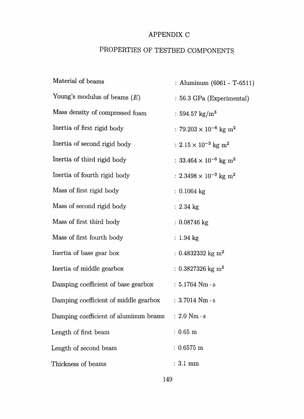
APPENDIX C

PROPERTIES OF TESTBED COMPONENTS

Material of beams

Young's modulus of beams {E)

Mass density of compressed foam

Inertia of first rigid body

Inertia of second rigid body

Inertia of third rigid body

Inertia of fourth rigid body

Mass of first rigid body

Mass of second rigid body

Mass of first third body

Mass of first fourth body

Inertia of base gear box

Inertia of middle gearbox

Damping coefficient of base gearbox

Aluminum (6061 - T-6511)

56.3 GPa (Experimental)

594.57 kg/m^

79.203 X 10-6 kg m2

2.15 X 10-3 kgm^

33.464 X 10-6 i g j^2

2.3498 X 10-3 kg m^

0.1064 kg

2.34 kg

0.08746 kg

1.94 kg

0.4832332 kg m^

0.3827326 kg m^

5.1764 Nm-s

Damping coeffîcient of middle gearbox : 3.7014 Nm • s

Damping coefficient of aluminum beams : 2.0 Nm • s

Length of first beam

Length of second beam

Thickness of beams

: 0.65 m

: 0.6575 m

: 3.1 mm

149

150

Width of beams : 38.24 mm

Coefficient of friction between tip of

manipulator and constraint surface : 0.5

Accelerometers

Manufacturer : PCB Piezotronics, Depew, NY

Model Number (Sensitivity) : 309A (5 mV/g)

: 352B68 (100 mV/g)

Signal Amplifier : 482A22 (4-Channel, Unity Gain)

Data Acquisition System

Manufacturer : lOTECH, Cleveland, OH

Model name and number : WaveBook/512

Number of inputs : 1 Digital and 8 Analog inputs

Maximum scan rate : 1 MHz

Motors, Gearboxes and Encoders

Motors

Manufacturer : Maxon Precision Motors, Switzerland

Xype : Permanent magnet DC motors

Model number : RE035-071-33EAB200A (90 watt) (Base motor)

: 2332.966-51-236-200 (15 watt) (Middle motor)

Gearboxes

151

Manufacturer : Maxon Precision Motors, Switzerland

Type : 3 Stage planetary gearhead

Gear reduction : 156 (Base gearbox)

Digital Encoders

: 236 (Middle gearbox)

Manufacturer : Hewlett-Packard, USA

Model : HEDS 5540 (Base encoder)

: HEDS 5500 (Middle encoder)

Coimts per turn : 500 (Both encoders)