Lauren M. Scott, PhD Lauren Rosenshein Bennett, MS

Modeling Spatial Relationships Using Regression Analysis

Workshop Overview Answering “why?” questions

• Introduce regression analysis - What it is and why you care - Example applications

• Work through solving a real problem using regression

Modeling variations in per capita Medicare spending

- Finding a properly specified OLS model

- The 6 things you must check!

- Exploring regional variation using GWR

- “What if?” scenarios - Identifying opportunities for

tailored remediation

What is Regression analysis?

• Model, examine, and explore spatial relationships

• Better understand the factors behind observed spatial patterns

• Predict outcomes based on that understanding

Ordinary Least Square e ry Least S

(OLS) Sqst S

))

20 40 60 80 100 0

20

0

40

60

80

100

Observed Values Predicted Values

Geographically Weighted d eographically WRegression

ly Wonon

WeighteWy Wnn (GWR

ghteRR)

ddedhteRR))

What’s the big deal?

• Pattern analysis (without regression): - Are there places where people persistently die young? - Where are test scores consistently high? - Where are 911 emergency call hot spots?

• Regression analysis: - Why are people persistently dying young? - What factors contribute to consistently high test scores? - Which variables effectively predict 911 emergency call volumes?

Regression analysis terms and concepts

• Dependent variable (Y): What you are trying to model or predict (e.g., residential burglary).

• Explanatory variables (X): Variables you believe cause or explain the dependent variable (e.g., income, vandalism, number of households).

• Coefficients (β): Values, computed by the regression tool, reflecting the relationship between explanatory variables and the dependent variable.

• Residuals (ε): The portion of the dependent variable that isn’t explained by the model; the model under- and over-predictions.

The asterisk * indicates the explanatory variable is statistically significant

Intercept 1.625506 INCOME -0.000030 VANDALISM 0.133712 HOUSEHOLDS 0.012425 LOWER CITY 0.136569

Regression model coefficients • Coefficient sign (+/-) and magnitude reflect each explanatory variable’s

relationship to the dependent variable

Why use regression?

• Explore correlations - Does higher Medicare spending translate to better

health or to better quality health care?

• Predict unknown values - How many claims for heat related illnesses can we

expect given current weather forecasts?

• Understand key factors - Why are people are dying young in South Dakota?

Explore Correlations

• Crime Analysis - Are you more likely to be robbed in a rich or

poor neighborhood? - Do we see more crime in neighborhoods

where there is more vandalism (“Broken Window” theory) or less vandalism?

Predictive Modeling

• Property values - If we have data for recent home sales,

can we predict home values?

• Demand for services - If we know the number of 911 calls is a

function of population, education, and jobs, can we use population projections to predict future demand?

Understand Key Factors

• Natural Resource Management - What are the most important habitat characteristics for an

endangered animal?

• Education - What are the key factors contributing to consistently high test

scores?

• Public Health - What variables most effectively explain high rates of childhood

obesity?

Lauren Rosenshein Bennett

OLS Regression

Why is Medicare Spending so o Why is Medicare SpHigh in the south?

peSp?? HigHig

Are people just sicker there?e?

The HCC index explained 66% % of the variation in the e per capita costs s The HCC index explained 66%% dependent variable: Adjusted R

% RR-

the variation in tf ofRR-Squared [2]:

thee in 0.656

ee epe5656 dede

However, significant spatial autocorrelation among model residuals s However, significant spatial autocorrelation among model residualsHo s indicates important explanatory variables are missing from the model.el.elel

OLS analysis

Build a multivariate regression model

• Explore variable relationships using the scatterplot matrix

• Consult theory and field experts

• Look for spatial variables

• Run OLS (this is iterative)

• Use Exploratory Regression

Our best OLS model

• Per capita Medicare costs as a function of: - Dehydration Admissions

- Hospital Beds

- Imaging Events

- Evaluation and Management Costs

- Distance to Houston

• This model tells 86% of the story… and the over and under predictions aren’t clustered!

But are we done?

Check OLS results 11 11 Coefficients have the expected sign.n.

22 222 No redundancy among explanatory variables.s.

33 333 Coefficients are statistically significant.t.

44 44 Residuals are normally distributed.d.

55 55 Residuals are not spatially y autocorrelateded.d.

66 66 Strong Adjusted RR-R-Square value.e.

1. Coefficient signs

• Coefficients should have the expected signs.

• Imaging Events per 1000 people +

• PQI10: Dehydration Admissions +

• Distance to Houston –

2. Coefficient significance • Look for statistically significant explanatory variables.

• Coefficients for all of the explanatory variables are statistically significant at the 0.05 level

• Since the Koenker test is statistically significant, we can only trust the robust coefficient probabilities

Check for variable redundancy

• Multicollinearity: - Term used to describe the phenomenon when two or more of

the variables in your model are highly correlated.

• Variance inflation factor (VIF):

- Detects the severity of multicollinearity. - Explanatory variables with a VIF greater than 7.5 should be

removed one by one.

3. Multicollinearity

• Find a set of explanatory variables that have low VIF values.

• In a strong model, each explanatory variable gets at a different aspect of the dependent variable.

• As a rule of thumb, VIF values should be smaller than 7.5.

Checking for model bias

• The residuals of a good model should be normally distributed with a mean of zero

• The Jarque-Bera test checks model bias

4. Model bias

• When the Jarque-Bera test is statistically significant: - The model is biased - Results are not reliable - Sometimes this indicates a key variable is missing from

the model

5. Model performance

• Compare models by looking for the lowest AIC value. - As long as the dependent variable remains fixed, the AIC value

for different OLS/GWR models are comparable

• Look for a model with a high Adjusted R-Squared value.

Statistically significant clustering of of Statistically significant clusterunder and over predictions.

risters.s

Random spatial pattern of underer Random spatial patterRaand over predictions

tternsns.

nrnterss. anan

6. Spatial Autocorrelation

Online help is … helpful!

The 6 checks: Coefficients have the expected sign. Coefficients are statistically significant. No redundancy among explanatory variables. Residuals are normally distributed. Residuals are not spatially autocorrelated. Strong Adjusted R2 (good model performance)

Also Helpful: Exploratory Regression

Are we done?

• A statistically significant Koenker OLS diagnostic is often evidence that Geographically Weighted Regresion (GWR) will improve model results

• GWR allows you to explore geographic variation which can help you tailor effective remediation efforts.

Global vs. local regression models

• OLS - Global regression model - One equation, calibrated using data from all features - Relationships are fixed

• GWR - Local regression model - One equation for every feature, calibrated using data from

nearby features - Relationships are allowed to vary across the study area

For each explanatory variable,e, For each explanatory variablGWR creates a coefficient

eeablt GWR creates a coefficienGWR creates a coefficient t

surface showing you where e surface showing you whesurface showing you wherelationships are strongest

ereress .reree estst.

Lauren Rosenshein Bennett, MS

Exploring Regional Variation

Running GWR

• GWR is a local spatial regression model

– Modeled relationships are allowed to vary

• GWR variables are the same as OLS, except:

– Do not include spatial regime (dummy) variables

– Do not include variables with little value variation

Defining local

• GWR constructs an equation for each feature

• Coefficients are estimated using nearby feature values

• GWR requires a definition for nearby

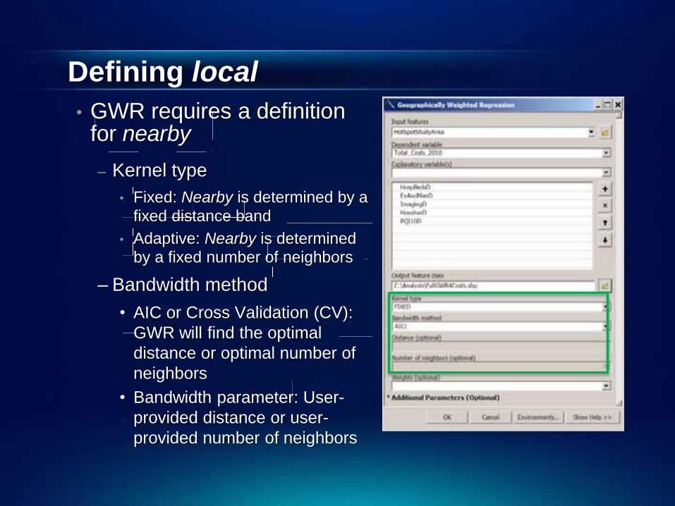
Defining local • GWR requires a definition

for nearby – Kernel type

• Fixed: Nearby is determined by a fixed distance band

• Adaptive: Nearby is determined by a fixed number of neighbors

– Bandwidth method • AIC or Cross Validation (CV):

GWR will find the optimal distance or optimal number of neighbors

• Bandwidth parameter: User-provided distance or user-provided number of neighbors

Interpreting GWR results

• Compare GWR R2 and AICc values to OLS R2 and AICc values - The better model has a lower AICc and a high R2.

• Model predictions, residuals, standard errors, coefficients, and condition numbers are written to the output feature class.

Mapped Output

• Residual maps show model under- and over-predictions. They shouldn’t be clustered.

• Coefficient maps show how modeled relationships vary across the study area.

Mapped Output

• Maps of Local R2 values show where the model is performing best

• To see variation in model stability:

apply graduated color rendering to Condition Numbers

GWR prediction

Predicted

Calibrate the GWR model using known n Calibrate the GWR model using knownnvalues for the dependent variable and all ll ll values for the dependent vvalues for the dependent variaof the explanatory variables

vavariaeses.

ababaaariaariass.

Provide a feature class of prediction n Provide a feature class of predictionnlocations containing values for all of the ee locations containing vlocations containing valuexplanatory variables.

ueuevaluvalus. s

GWR will create an output feature class s GWR will create an output featuwith the computed predictions

eatunsns.

reuratuss.

Observed Modeled

Resources for learning more…

• www.esriurl.com/spatialstats - Short videos

- Articles and blogs

- Online documentation

- Supplementary model and script tools

- Hot spot, Regression, and ModelBuilder tutorials

• resources.arcgis.com

LBennett@Esri.com LScott@Esri.com

QUESTIONS?