MODELING STRATEGIES FOR A GROUNDWATER DOMINATED HEADWATER SYSTEM

1Latif Kalin, 1Rasika Ramesh, 2Mohamed Hantush, 3Mehdi Rezaeianzadeh, 1Chris Anderson,

1 School of Forestry and Wildlife Sciences, Auburn University, Auburn, Alabama2 National Risk Management and Research Laboratory, US Environmental Protection Agency, Cincinnati, Ohio3 National Water Center, National Oceanic and Atmospheric Administration, Tuscaloosa, Alabama

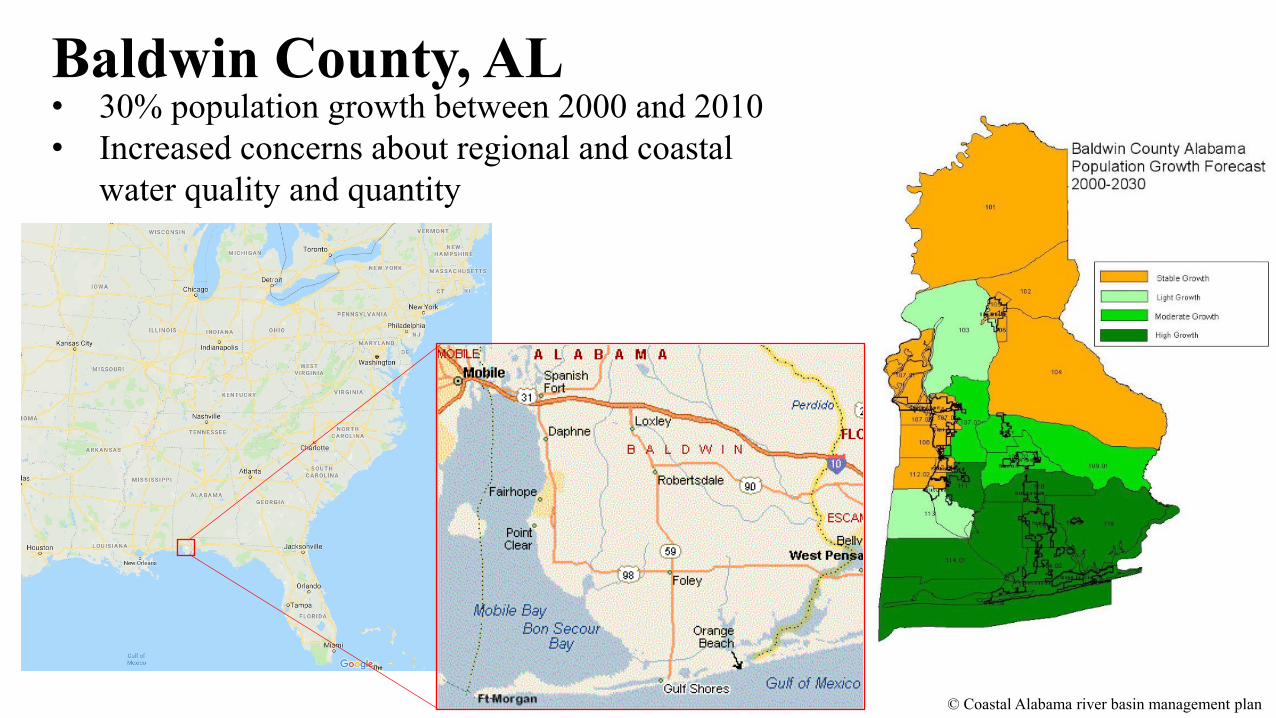
Baldwin County, AL

© Coastal Alabama river basin management plan

• 30% population growth between 2000 and 2010• Increased concerns about regional and coastal

water quality and quantity

“Headwater streams are buried more extensively than are larger streams at all levels of urban development (low, residential, suburban, and urban)” – Elmore and Kaushal (2008)

Wetland alterations

Watershed land use is an important driver of wetland function

-70

-60

-50

-40

-30

-20

-10

0

10

2/27/2011

2/28/2011

3/1/2011

3/2/2011

3/3/2011

3/4/2011

3/5/2011

3/6/2011

3/7/2011

3/8/2011

3/9/2011

3/10/2011

Wat

er le

vel d

epth

(cm

) re

l. to

gro

und

leve

l

55% Forested

87% Urban

Headwater wetland

Baldwin County, AL

• Account for over two-thirds of the total stream length in a river

• Alterations can cause large scale impacts on ecological functions

Headwater slope wetlands

Study areas

Increasingly urban watershedsSouth North

The general plan

Improved water quality prediction

SWATWatershed model

•Land use•Climate •Soils

WETQUALWetland model

•Flow•Nutrients•Climate

Flow and nutrient time series Calibrate with observed wetland data

New Foley watershed

• Head watershed draining into headwater slope wetland (yellow star in map)

• Ungauged• Stage data at discernible

inflow from Aug 2013 – May 2014

Temperature stationWatershed outlet

0

0.1

0.2

0.3

0.4

0.5

0.6

Flow

(cm

s)

Observed inflow to wetland SWAT generated flow to wetland

Observed data

On inspection…

Watershed size = 0.49 sq.kmPrecipitation = 1723 mmTotal flow = 6599 mm

Where was all this extra water coming from?

0

20

40

60

80

100

120

140

Flow

dep

th (m

m)

Precipitation Flow

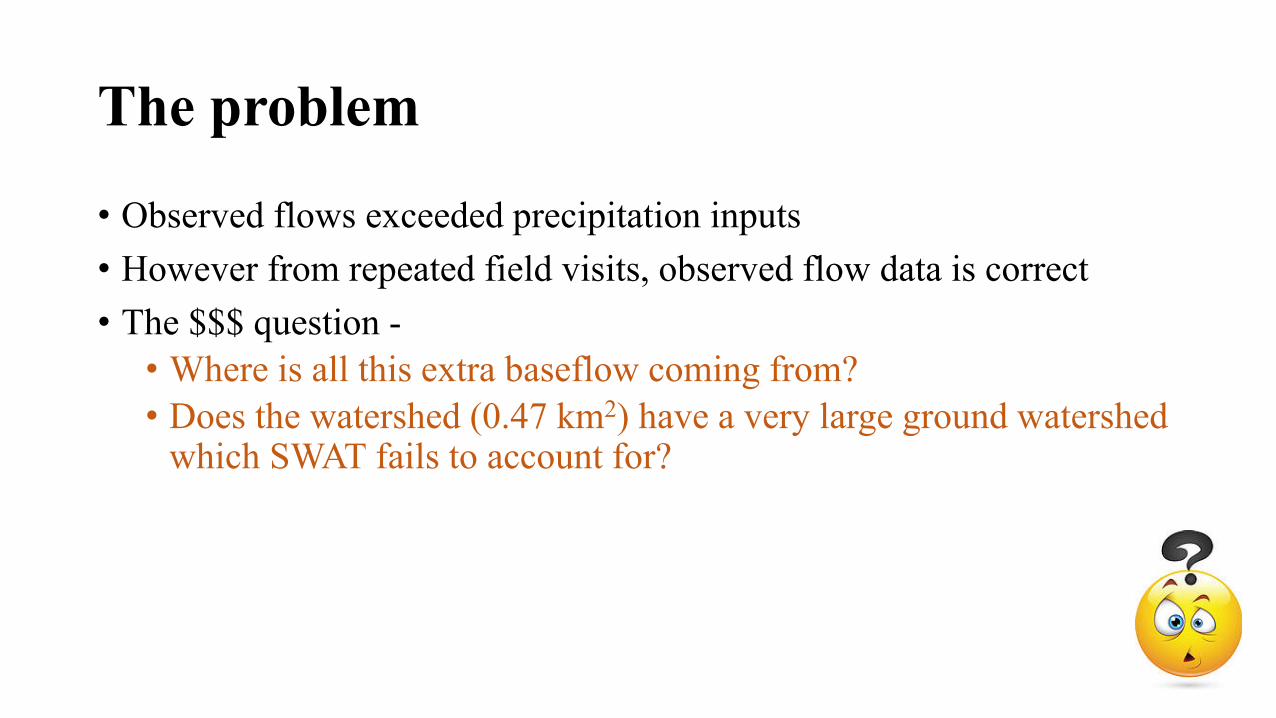
The problem

• Observed flows exceeded precipitation inputs• However from repeated field visits, observed flow data is correct• The $$$ question -

• Where is all this extra baseflow coming from?• Does the watershed (0.47 km2) have a very large ground watershed

which SWAT fails to account for?

Objectives

• Can flows be modeled in SWAT relatively simply without having to resort to complex groundwater models?

• Provide useful approaches using SWAT model to predict flows in small watersheds with extensive ground watersheds

11

Topo map

0

0.1

0.2

0.3

0.4

0.5

Flow

(cm

s)

Observed Stormflow SWAT simulated streamflow

0

0.05

0.1

0.15

0.2

0.25

Flow

(cm

s)

Observed baseflow SWAT simulated baseflow

Taking a closer look..

ENASH = -5.6 ENASH = 0.44

Approach 1

From the data,

SWAT streamflow + [a + (b * SWAT baseflow)] ≅ Observed streamflow

Linear regression

0

0.004

0.008

0.012

0.016

0.02

0

0.05

0.1

0.15

0.2

0.25

0.3

SWAT

sim

ulat

ed b

asef

low

(cm

s)

Obs

erve

d ba

seflo

w (c

ms)

Observed baseflow SWAT simulated baseflow

Calibrating baseflow trendImportant SWAT parameters:GWDELAY = 1 dayRCHRGE_DP = 0

Observed baseflow = 13.352 * Simulated baseflow – 0.0038(R2 = 0.75)

y = 13.352x - 0.0038R² = 0.7533

0

0.05

0.1

0.15

0.2

0.25

0.3

0 0.005 0.01 0.015 0.02

Obs

erve

d ba

seflo

w (c

ms)

Trend calibrated baseflow simulated by SWAT (cms)

Observed baseflow (cms)Linear (Observed baseflow (cms))

Calibrating stormflow

0

0.1

0.2

0.3

0.4

0.5

Flow

(cm

s)

Observed stormflow SWATCUP calibrated streamflow

(R2 = 0.71, ENASH = 0.62)

Parameter_Name Fitted_Value 1: r__CN2.mgt 0.015 2: v__ALPHA_BF.gw 0.690 3: v__GW_DELAY.gw 0.362 4: v__GWQMN.gw 21.741 5: v__GW_REVAP.gw 0.199 6: v__ESCO.hru 0.842 7: v__CH_N2.rte 0.224 8: v__CH_K2.rte 32.122 9: v__ALPHA_BNK.rte 0.884 10: r__SOL_AWC(..).sol -0.151 11: r__SOL_K(..).sol 0.014 12: r__SOL_BD(..).sol -0.809 13: v__RCHRG_DP.gw 0.006

0

0.1

0.2

0.3

0.4

0.5

0.6

0.7

8/4/2013 9/23/2013 11/12/2013 1/1/2014 2/20/2014 4/11/2014

Flow

(cm

s)

Observed streamflow (cms) SWAT simulated streamflow (cms)

Calibrated baseflow + calibrated stormflow

0

0.1

0.2

0.3

0.4

0.5

0.6

0 20 40 60 80 100

Flow

(cm

s)

Percent of time equaled or exceeded

Observed streamflow (cms)

SWAT simulated streamflow (cms)

Predicted flow = 13.352 * trend calibrated baseflow – 0.0038 + calibrated stormflow(R2 = 0.74, ENASH = 0.67)

Approach 2

Baseflow

Recharge to aquifer wrchrg

When β > 0 When β < 0

Deep aquifer recharge wdeep = βdeep.wrchrg

Total shallow aquifer recharge, wrchrge,sh

Shallow aquifer

Deep aquifer

• In SWAT, RCHRGE_DP (βdeep) ranges from 0 to 1

- only considers percolation loss to deep aquifer

Calibrate with negative RCHRGE_DP

Parameter_Name Fitted_Value Min_value Max_value 1: r__CN2.mgt 0.285 0.126 0.421 2: v__ALPHA_BF.gw 0.082 0.001 0.173 3: v__GW_DELAY.gw 0.563 0.001 3.104 4: v__GWQMN.gw 41.312 25.939 43.589 5: v__GW_REVAP.gw 0.094 0.026 0.101 6: v__ESCO.hru 0.952 0.916 0.985 7: v__CH_N2.rte 0.144 0.125 0.254 8: v__CH_K2.rte 131.781 85.332 142.185 9: v__ALPHA_BNK.rte 0.386 0.232 0.740 10: r__SOL_AWC(..).sol -0.435 -0.441 -0.068 11: r__SOL_K(..).sol 0.241 -0.098 0.442 12: r__SOL_BD(..).sol 0.029 -0.217 0.134 13: v__RCHRG_DP.gw -15.293 -19.559 -13.066

00.10.20.30.40.50.6

0 20 40 60 80 100

Flow

(cm

s)

Percent of time equaled or exceeded

Observed streamflow (cms)SWAT simulated streamflow (cms)

(P-factor = 0.84, R-factor = 1.04, R2 = 0.78, ENASH = 0.75

SWAT+ANN for improved calibration

0

0.1

0.2

0.3

0.4

0.5

0.6

0.7

8/4/2013 9/23/2013 11/12/2013 1/1/2014 2/20/2014 4/11/2014

Flow

(cm

s)

Observed streamflow SWAT-ANN simulated streamflow

00.10.20.30.40.50.6

0 50 100

Flow

(cm

s)

Percent of time equaled or exceeded

Observed streamflow (cms)SWAT simulated streamflow (cms)

SWAT calibrated flow + ET + Precipitation = Improved hydrology prediction1 hidden layer, 8 nodes, log-sigmoid transfer functionENASH = 0.89

20

Results and conclusions

• Evaluated approaches for SWAT application in groundwater dominant watersheds

• Useful SWAT parameter tweak to model high groundwater systems without having to resort to complex groundwater models

• SWAT+ANN is a very useful tool for superior hydrology calibration