modeling the climatic and subsurface … difﬁcult to determine if the wetland hydrology ob-served...

567

WETLANDS, Vol. 26, No. 2, June 2006, pp. 567–580q 2006, The Society of Wetland Scientists

MODELING THE CLIMATIC AND SUBSURFACE STRATIGRAPHY CONTROLSON THE HYDROLOGY OF A CAROLINA BAY WETLAND IN

SOUTH CAROLINA, USA

Ge Sun1, Timothy J. Callahan2, Jennifer E. Pyzoha3,5, and Carl C. Trettin4

1Southern Global Change Program, Southern Research Station, USDA Forest Service920 Main Campus, Venture II, Suite 300

Raleigh, North Carolina, USA 27606E-mail: [email protected]

2Department of Geology and Environmental GeosciencesCollege of Charleston

66 George StreetCharleston, South Carolina, USA 29424

3Master of Environmental Studies ProgramCollege of Charleston

66 George StreetCharleston, South Carolina, USA 29424

4Center for Forested Wetlands ResearchUSDA Forest Service

2730 Savannah HighwayCharleston, South Carolina, USA 29414

5Present AddressAMEC Earth & Environmental

659 N High StreetColumbus, Ohio, USA 43085

Abstract: Restoring depressional wetlands or geographically isolated wetlands such as cypress swamps andCarolina bays on the Atlantic Coastal Plains requires a clear understanding of the hydrologic processes andwater balances. The objectives of this paper are to (1) test a distributed forest hydrology model, FLAT-WOODS, for a Carolina bay wetland system using seven years of water-table data and (2) to use the modelto understand how the landscape position and the site stratigraphy affect ground-water flow direction. Theresearch site is located in Bamberg County, South Carolina on the Middle Coastal Plain of the southeasternU.S. (32.888 N, 81.128 W). Model calibration (1998) and validation (1997, 1999–2003) data span a wetperiod and a long drought period, which allowed us to test the model for a wide range of weather conditions.The major water input to the wetland is rainfall, and output from the wetland is dominated by evapotrans-piration. However, the Carolina bay is a flow-through wetland, receiving ground water from the adjacentupland, but recharging the ground-water to lower topographic areas, especially during wet periods in wintermonths. Hypothetical simulations suggest that ground-water flow direction is controlled by the gradient ofthe underlying hydrologic restricting layer beneath the wetland-upland continuum, not solely by the topo-graphic gradient of the land surface. Ground-water flow may change directions during transition periods ofwetland hydroperiod that is controlled by the balance of precipitation and evapotranspiration, and suchchanges depend on the underlying soil stratigraphy of the wetland-upland continuum.

Key Words: wetland hydrology, ground water, Carolina bays, modeling, geomorphology

INTRODUCTION

Depressional wetlands, or geographically isolatedwetlands, such as cypress (Taxodium ascendensBrongn.) swamps and Carolina bays, are common landfeatures in the Atlantic Coastal Plain of the southeast-

ern U.S. (Tiner et al. 2002). They vary in size fromless than a hectare to more than several hundred hect-ares. Depressional wetlands may be undisturbed for along period of time, but their surrounding ‘uplands’are often managed for timber or agricultural produc-tion due to drier soil conditions. These wetlands occur

568 WETLANDS, Volume 26, No. 2, 2006

on flat topography between river divides and have noapparent surface-water connections with rivers orlakes. However, in locations where the water-table isclose to ground surface, depressional wetlands can be-come temporarily connected to other water bodiesthrough overland sheet flow (Winter and LaBaugh2003). Shallow ground-water flow also links the sur-face-water in the wetland to its surrounding upland,especially when the entire landscape is wet, such as inthe winter months (Sun et al. 2000).

Although isolated wetlands, like many other typesof wetlands, play important roles in providing wildlifehabitats (Sharitz 2003), ground-water recharge, waterquality improvement, and carbon sequestration (Li etal. 2003), they are under enormous stress from bothland development and climate change and variability(U.S. Global Change Program 2000). Understandingtheir hydrologic processes is one of the keys to wet-land restoration and management (De Steven and Ton-er 2004). Wetland hydrology of depressional wetlands,as controlled by water levels within the wetland andsurrounding uplands, is complex because of the dy-namic nature of ground-water and surface-water inter-actions (Sun et al. 2000; Bliss and Comerford, 2002).The hydrogeomorphic (HGM) wetland classificationscheme (flat, depressional, riverine, etc.) stresses theimportant topographic and geologic control on wetlandhydrology at a landscape scale (Brinson 1993). Lideet al. (1995) found that ground-water-surface-water in-teractions were variable depending on both climateand local soil layering and geology, but few studieshave explicitly explored the causes of the interactions.In a hydrologic study on cypress swamps in north-central Florida, USA, Sun et al. (2000) suggested thatlateral ground-water-surface-water interactions werecommon, but the largest fluxes were during the wet-dry transition periods, whereas the hydraulic gradientswere reduced during both dry and wet periods. Theyconcluded that the interactions between ground waterand surface-water in wetlands were not well connectedto the deeper aquifers, and thus, vertical exchange ofground water was not common.

While field investigations provide many insightsinto the complex interactions among climate, surface-water, ground-water, and surface and subsurface soils,they are often time-consuming and expensive. It is of-ten difficult to determine if the wetland hydrology ob-served during the monitoring period is actually typicalfor the region. Computer simulation models can behelpful in determining the detailed processes and flux-es of water flows over both space and time by lessexpensive means and at scales that are not feasiblewith field experiments. Furthermore, a well validatedmodel can be used to answer ‘what if’ managementquestions (Skaggs et al. 1991). For depressional wet-

lands, water-table levels are essentially controlled bytwo types of fluxes, one in the vertical direction (pre-cipitation and evapotranspiration) and another in thelateral direction (shallow ground-water flows). Thus,this requires a multi-dimensional model to describefully the hydrology of depressional wetlands (Mansellet al. 2000). A comprehensive model that captures thefull hydrologic cycle also acts as an integration tool tolink all variables and hydrologic fluxes measured at aresearch site and is useful to identify gaps in monitor-ing.

Several hydrologic models are available for mod-eling the water budgets of wetland ecosystems in thesouthern U.S. The most widely used is the lumpedDRAINMOD model (Skaggs et al. 1991) that was de-signed for and is most applicable to drained flat land-scapes with parallel ditches. The model can simulatethe spatial distribution of water-table dynamics of each‘drained field’ but is limited in describing explicitlythe hydrologic interactions of surface water andground water in a wetland-upland system. The WET-LANDs model (Mansell et al. 2000) describes the hy-drology of a wetland-upland system by the combina-tion of 2-D Richard’s equation and the water balancein wetland. This model has the capability to includethe heterogeneity of both geology/soils and land cover.Other lumped wetland hydrology models, such asSWAT (Arnold et al. 2001) and Soil Water BalanceModel (Walton et al. 1996 cited in Arnold et al. 2001),cannot simulate the lateral interactions of surface-wa-ter and ground-water interactions at the interface be-tween a wetland and its upland.

The overall goal of this study was to use a computermodel as an alternative tool to understand the hydro-logic processes in Carolina bays. Specially, the objec-tives of this paper were (1) to test and validate a dis-tributed forest hydrology model, FLATWOODS, for aCarolina bay wetland system using seven years of wa-ter-table data and (2) to apply the validated model topredict the effects of climate and subsurface soil lay-ering or stratigraphy on lateral ground-water flow di-rections (i.e., ground-water and surface-water interac-tions).

METHODS

The FLATWOODS Model

The FLATWOODS forest hydrology model wasoriginally developed for the flatwoods ecosystems, amosaic of cypress swamps and slash pine uplands ofFlorida, U.S.A, a region dominated by poorly-drainedsoils, low topographic relief, and high precipitationand evapotranspiration rates (Sun et al. 1998a, b). Theadvantages of using this model in other locations of

Sun et al., MODELING THE CLIMATIC AND ..... 569

Figure 1. Sketch of the FLATWOODS model structure and hydrologic components.

the Southeastern U.S. are 1) it has been validated forhumid, warm, poorly drained forested conditions, and2) it is a distributed model that simulates the completehydrologic cycle of both a wetland and its surround-ings, including evapotranspiration, vertical soil-waterflow (infiltration and soil moisture redistribution), andlateral ground-water flow in a shallow unconfinedaquifer. Most importantly, the model can explicitlysimulate the hydrologic interactions between a wetlandand upland through the lateral ground-water-flow com-ponent. The FLATWOODS model includes three ma-jor submodels, or modules, to simulate the spatial dis-tribution of ground-water-table and hydrologic fluxes.At a gridded ‘cell’ level, the evapotranspiration mod-ule simulates daily water loss due to forest canopyinterception, plant transpiration, and soil/water evap-oration as a function of potential evapotranspiration,rooting depth, and plant growth stage. Daily potentialevapotranspiration rate is calculated by Hamon’smethod (Hamon 1963) as a function of air temperatureand day light hours (Fedder and Lash 1978). The un-saturated water-flow module uses a simple water-bud-get algorithm to estimate recharge to the shallowground-water system beneath the unsaturated soil

zone. Recharge was calculated as the surplus of dailynet precipitation data (atmosphere precipitation—can-opy interception) above soil-water field capacity. In-filtrated water first fills up the available storage of theunsaturated zone before recharging the surficial aqui-fer. The ground-water-flow module is the core of themodeling system. This module tracks the water- tablehydraulic head of each gridded cell using a 2-D (x andy) ground-water-flow algorithm that simulates the wa-ter-table fluctuations as a function of evapotranspira-tion loss from the aquifer, water loss due to surfaceoutflow, recharge to shallow aquifers, and water loss/gain from surrounding neighbor cells. Surface outflowoccurs only when the ground-water table reaches theground surface. Surface water is allowed to move outof the model boundary in one time step (one day). Themodel structure is presented in Figure 1 to illustratethe modeling components and interactions of waterfluxes in a wetland-upland landscape. Details of modelalgorithms, model validation, and application in pineflatwoods are found in Sun et al. (1998a, b). Key mod-el input and output variables and calibrated soil param-eters are listed in Table 1.


Table 1. Major model inputs and outputs of the FLATWOODS hydrologic model.

Model Overview Variables and Parameters

Input requirements Climate Measured daily precipitation, average air temperature for estimating poten-tial evapotranspiration calculated using Hamon’s method (Hamon 1963;Federer and Lash 1978)

Vegetation Deciduous in the wetlands and uplands; leaf areas vary with time with can-opy interception rates reported by Helvey and Patric (1965). Leaf outdate starts April 1 to full April 30, and leaf drop starts November 1 andends November 30 according to field observation.

Soils Hydrologic restricting layer depth 4.0 and 3.0 m below ground for uplandand wetland respectively; hydraulic conductivity: 3.7 m/day for upland;0.37 m/day for wetland. Specific Yield: 0.05; porosity 0.35; plant wiltingpoint 0.15 for both wetland and upland (parameter calibrated from initialvalues provided in the report by USDA SCS (1966).

Ouputs Daily canopy interception, transpiration, soil evaporation, soil moisture content (%), ground-water-tabledepth.

Study Site and Field Data Acquisition for ModelTesting

The research site is in Bamberg County, South Car-olina on the Middle Coastal Plain of the SoutheasternU.S. (32.888 N, 81.128 W). Long-term (1951–2004)annual average air temperature and total precipitationin the region are 17.9 8C and 1210 mm, respectively(Southeast Regional Climate Center 2005). The pre-cipitation patterns can be greatly influenced by tropicalstorms between the months of July and October whendaily extremes are most likely to occur (Southeast Re-gional Climate Center 2005). A standard weather sta-tion at the study site recorded precipitation with a tip-ping bucket raingage and air temperature with a tem-perature probe (Campbell Scientific, Inc., Logan, UT).When on-site weather data were missing due to equip-ment failure, data collected at the Bamberg Countyweather station about 25 km from the study site wereused.

Three Carolina bay ecosystems have been exten-sively monitored since 1997 by Pyzoha (2003). Thismodeling study focused only on Chapel Bay, one ofthe three intensively monitored Carolina Bay wetlands.We briefly describe methods employed in derivingvarious model parameters. Selected ground-water-tabledatasets are presented for justifying model setups forboundary conditions and evaluating model perfor-mance in calibration, validation, and application. De-tailed field installation and data summary are reportedby Pyzoha (2003).

The Chapel Bay wetland studied herein has an areaof about 8 ha covered mostly by deciduous bottomlandhardwood plants including water oak (Quercus nigraL.), willow oak (Q. phellos L.), black cherry (Prunusserotina Ehrh), swamp tupelo (Nyssa biflora Walt.),sweet gum (Liquidambar styraciflua L.), loblolly pine(Pinus taeda L.) and some pond cypress (Taxodium

ascendens) in the interior. During the field data col-lection period of 1997–2003, the land-use types sur-rounding the Carolina bay were composed of croplands, intensively-managed, short rotation hardwoodplantations of sycamore (Acer pseudoplatanus L.) andcottonwood (Populus deltoides Bartr. ex Marsh.) andnatural pine stands. The soil in the wetland is typifiedby poorly drained sandy loams, while wetland-uplandmargins and the uplands are dominated by betterdrained loamy sand or deep sandy soils (USDA SCS1966).

Small changes of surface elevation will alter sur-face-water flow directions in this relatively flat land-scape. Although a Digital Elevation Model (DEM)with a 30-m resolution is available, the surface ele-vations of the wetland and its surrounding area wereresurveyed to a precision of 1.5 mm at 30-m mea-surement distance and geo-referenced into a 100-m by100-m grid system for model setup and validation(Trimble Spectra Precision Laser Level, Trimble Nav-igation, Ltd., Sunnyvale, CA) (Figure 2). The highestelevation is in the northwest corner and the lowest inthe south edge of the wetland. A highway (Highway301) intersects with wetland at the southeast corner.Field inspection found several storm drains that con-nect the roadside ditches on both sides of the highway.Although the wetland has a berm at the dissected sideof the wetland, field evidence suggested that surfacewater could flow over the barrier when the wetland isfull.

The general stratigrahy of the wetland and surround-ing upland area was determined from logs to approx-imately 10 m during well and piezometer installation.Water-table wells were constructed from PVC or stain-less steel piping screened the entire length and in-stalled to a depth up to 2.5 m. Piezometers were con-structed with PVC pipes with a diameter of 3.8–5.1


Figure 2. Model grid (100 m by 100 m) setup and surface elevation (a), and sketch of instrumentation (not to scale) (b), atthe Chapel Bay research site.


cm with a porous ceramic cup sealed at the bottomand were installed to a depth up to 3.5 m and 9 mdeep in the wetland and upland, respectively. In Chap-el Bay and surrounding area, 21 wells and 24 piezom-eters were employed during different periods of theseven-year field study. Selected well or piezometerdata were used in this study to justify model setupsand validation. Complete data description was foundin Pyzoha (2003).

Saturated hydraulic conductivity was determined byslug and bail tests (Bouwer and Rice 1976). Hydraulicconductivity values were measured in the range of1.2–5.4 m/day for upland sediments with the wellscreen at about 4.5 m below the ground surface. Slugtests were not successful in wetlands, but the sedi-ments in wetlands were suspected to have lower hy-draulic conductivity values because of their greaterclay contents. Hydraulic conductivity of wetland soilswith sandy loams and sandy clay loams have a rangeof 0.5–1.5 m/day (USDA SCS 1966). A clay layerabout 1–1.5 m below ground and up to 1 m thick wasobserved in Chapel Bay during well installation. Incontrast, two clay layers were found (from 2.75 to 4.75m and from 4.5 m to 7.5 m depth), with the formerlayer rather thin (0.2–0.5 m). It appears that uplandshave a thicker surficial aquifer with higher hydraulicconductivity, while the wetland portion of the land-scape has an aquitard closer to the ground surface andis poorly drained. The surficial aquifer in the area thatmost likely affects the hydroperiod of the wetland isthe top 5 m soil layers.

In addition to the 45 manual water-table wells andpiezometers around Chapel Bay as described above, adigital recording well (WL40) was installed to a depthabout 0.5 m to record water-table level continuouslyduring the entire study period (1997–2003). This shal-low well was located in the lowest area of the wetland(i.e., having standing water more often) and had thelongest recording history. Hydraulic head data mea-sured by three piezometers and the WL40 well wereused in this study to provide evidence that the 0–5 maquifer was unconfined.

The year 1998 was marked by an extremely wetspring but a dry summer and autumn. Therefore, thisyear was selected for model calibration to test themodel under a wide range of water-table conditions,and the rest of the water-table data from 1997 and1999–2003 were used for model validation (Figure 2).Starting from 1999 through fall 2002, the research siteexperienced severe-extreme draught conditions, with a330-mm deficit in annual precipitation.

The entire modeling system was divided into 49 1-ha cells. Lateral model boundary conditions were ini-tially determined by the road networks as a first ap-proximation of the flow regime. For example, several

cells of the lower southeast corner of the simulationgrid system were assumed to have no flows becauseof intersection with the highway (Highway 301). Thevertical flow boundary was determined from the stra-tigraphy data and comparison of hydraulic head in thepaired shallow wells and piezometers. Piezometerswere installed deeper than the shallow wells. We se-lected three representative piezometers and one shal-low well (WL40) to determine the bottom flow bound-ary and whether the ground-water system is artesian,confined, or unconfined. Initial conditions of the modelon water-table depth were approximated using themeasured hydraulic head data from the wetland andupland wells.

Model performance was first evaluated by graphi-cally comparing simulated daily water-table level atparticular modeling cells in the wetland (Cell 18, 19,26) and upland (Cell 17, 12) (Figure 2a) and measuredvalues at shallow wells located in those cells in 1998.Initially, a no-flow boundary condition was set for allthe modeling boundaries because no apparent overlandoutflow was recorded or observed by the field study.After the model was properly calibrated, the modelwas validated by comparing measured water level atwell WL40 and simulated for cell 19 during 1997–2003. The same set of soil and vegetation parameterswas used during model calibration and validation pe-riods.

RESULTS

Field Evidence of an Unconfined Aquifer Systemand General Ground-Water Flow Directions

Hydraulic heads measured at one transect (EF) bypiezometers at the upland (EE, 4.6 m below groundsurface), wetland-upland margin (EF22, 2.5 m belowground surface), and the wetland center (2.5 m deepfor the piezometer CT3 and 0.5 m for well WL40)provided important information of ground-water flowdirections in the lateral and vertical directions (Figure3). First, it appears that the observed clay layer at adepth of 1.5 m in the wetland did not result in anartesian effect since the hydraulic heads measured bythe wetland piezometer (CT3) at a depth of 2.5 m weresimilar to those of the shallow wells of WL40, espe-cially during wet periods. Small differences were no-ticed during dry-wet transition periods (e.g., middle2002). Thus, for modeling purposes, it is reasonableto approximate the entire bay ground-water system asan unconfined aquifer with a hydrologic restrictinglayer at about 2 m in the wetland and about 4 m inthe upland. Secondly, ground-water recharge from thesurrounding upland to the wetlands was mostly pro-nounced during the wet periods in the winter months


Figure 3. Measured water-table elevation (i.e., total hydraulic head) data at the upland, wetland-upland margin, and in thewetland indicates that the Chapel Bay is an unconfined aquifer system.

of 1998 and spring and summer of 2003. A maximumof about 1 m hydraulic head difference was measuredbetween the upland piezometer (EE) and the piezom-eter (CT3) and well (WL40) located in the wetland.The difference of surface elevation between the twopoints was about 2.4 m, and they were about 100 mapart.

Model Calibration and Validation

We found that the model greatly over-estimated thewater-table elevations for all the wells when a no-flowboundary condition was used (Figure 4a). A close ex-amination of the water-table data recorded by the au-tomatic water-table wells found that the wetland water-level rose very slowly when the water-level elevationreached about 54 m above mean seal level (msl). Thisphenomenon suggested that significant shallowground-water outflow and/or fast surface flow from thewetland might have occurred, and thus, the no-flowboundary assumption was not appropriate. A field in-spection confirmed our suspicion that surface outflowmight have occurred at the south corner of the wetlandduring extreme wet conditions. The storm-water drainbeneath Highway 301 might have exerted influence onthe wetland flow regime. Consequently, a constant-head flow boundary condition was imposed allowingground-water flow out of the boundary cells when thewater-table reached 54 m msl. This change greatly im-proved model performance (Figure 4b). Soil specificyield was also adjusted to achieve overall best fit to

the measured data. When surface-water was present inthe wetland, specific yield was raised to a maximumof 1.0. The adjusted correlation coefficient for aver-aged measurements and model predictions for the threewetland wells was R2 5 0.78 with the regression equa-tion (Simulated Hydraulic Head in m 5 0.704 * Mea-sured Hydraulic Head 1 15.8, n5274). For uplandcells, the model captured the wet-dry cycle of ground-water-table (R2 5 0.72 for the upland cell 17), yet themodel over-estimated the water-table levels, especiallyfor upland cell 12 (Figure 4b). The regression equationfor cell 17 calibration was determined as SimulatedHydraulic Head in m 5 1.389 * Measured HydraulicHead 221.35, n59).

In general, the model captured the water-table fluc-tuations reasonably well during the seven-year vali-dation period (Figure 5). The model simulated the fullwet-dry cycles of the wetland water level and alsomatched the maximum values. However, the modeloverestimated water levels during the transition peri-ods from a wet to a dry condition, such as the Fall1998 and Summer 2001, when the system presumablyhad a large water loss through evapotranspiration.Simulation errors were most pronounced when the wa-ter-table levels were in the low range, about 0.5 mbelow the ground surface (elevation 53.5 m) (Figure5 and Figure 6), and the discrepancy between modeledand measured values was the smallest when the wet-land becomes flooded (elevation .53.5 m). Thus, webelieve that soil parameters (specific yield) and theevapotranspiration submodels are critical to simulate


Figure 4. Model calibration using a) a no flow boundary and b) a fixed-head (54 m a.s.l.) boundary condition suggests thatChapel Bay is not hydrologically isolated from the surrounding upland and that lateral ground-water- surface-water interactionsare common.

the dynamics of wetland hydroperiod accurately. Onthe other hand, the accuracy of precipitation data isequally important to model validation. In fact, thismodeling study used climate data recorded at localcounty weather station when on-site data were missingfor part of year 2000. Thus, model results may be sus-pect for late 2000 and early 2001 (Figure 5) due toprecipitation data problems.

The annual water budgets show that precipitation

and evapotranspiration are the two major fluxes in theoverall water budgets (Figure 7). During wet years(1997 and 1998) when annual precipitation was abovethe 30-year average (1230 mm), net flows (surface-and ground-water flow) might be a significant flux inthe wetland water balance. During the drought years(2000–2002), evapotranspiration was nearly balancedwith precipitation at an annual scale, although periodicsurface water was present during those years (Figure


Figure 5. A seven-year model validation suggests that the wetland hydroperiod is mostly controlled by climate variabilityand that it can recover from extended drought rather quickly.

6). The modeling results reported here did not separatenet surface flow and net ground-water (i.e. water ex-change through wetland boundaries). The majority ofthe net flow in Figure 6 was surface outflow sincethere was no overland flow input and ground-waterinput and output probably balanced.

Model Applications

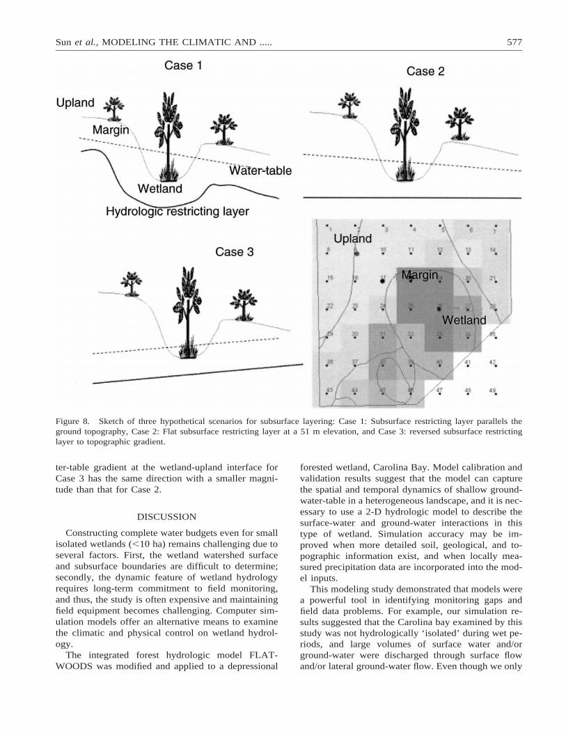
Once the model was reasonably validated, it wasapplied to test one hypothesis that has important im-plications to constructed wetlands. This study testedthe hypothesis that lateral ground-water flow directionat the upland-wetland boundary is determined by thesubsurface gradient of the hydrologic restricting layer,rather than solely by the ground topographic gradient.Therefore, two additional scenarios (Case 2 and Case3) were hypothetically constructed to evaluate twopossible subsurface soil layering scenarios as varia-tions of the reference natural condition (Case 1) (Fig-ure 8). For Case 1, the wetland is in the depressionarea and the subsurface clay layer follows a similar,but subdued gradient as the topography. Case 2 rep-resents a scenario where a flat hydrologic restrictinglayer (elevation of 51.0 m) occurs beneath the surficialaquifer, while Case 3 represents a scenario in whichthe subsurface gradient is the opposite of the land to-pographic gradient, with a slope set as about 0.13%.The three scenarios have the same land topography.The ground-water flow directions were determined bycomparing the total hydraulic head (i.e., water-levelelevations) at the three selected points: upland, upland-wetland margin, and wetland (Figure 8). The 12-yearclimate data series was constructed by repeating the

1997–2002 climate file twice to represent an extendedwet-dry climatic cycle.

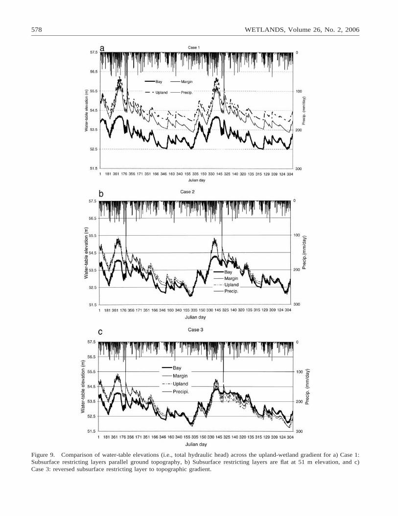
For Case 1, simulated water-table elevations suggestthat ground-water flow is in the upland-margin-wet-land direction, which is similar to the topographic gra-dient, throughout the 12 synthetic climate years (Fig-ure 9a). The upland-wetland water-table gradients arelarger during wet periods (winter months) than thoseduring dry periods (summer and autumn months). Thewetland receives ground-water discharge from the sur-rounding uplands, and it is a water ‘sink.’

Compared to Case 1, water-flow directions changegreatly in Case 2 (Figure 9b). Notably, the hydraulicgradients between upland and the margin are muchsmaller throughout the simulation period. The initialupland-wetland hydraulic gradient is caused by the ini-tial water-table conditions. The water-table gradientbetween the upland and the wetland diminishes towardthe end of a dry cycle but reappears during the wetwinter period and following several storm events. Dur-ing the following dry period, there is a small ground-water gradient in the wetland-upland system. A thickerunsaturated zone is developed in the upland than thewetland due to the fact that the upland ground surfaceis relatively higher than that of wetland for Case1.

The water-table gradient from the upland to the wet-land for the Case 3 scenario is similar to Case 2 in thefirst climatic cycle (Figure 9c), but some differencesbetween the two cases are obvious during the wettingphase of the climatic cycle. Except for the extreme wetperiod, the simulated water level in the depressionalwetland is constantly higher than at the margin andupland, creating a small reversal of hydraulic gradientagainst the topography. During the wet period, the wa-


Figure 6. Comparison of simulated and measured water-table elevation (i.e., total hydraulic head) at Chapel Bay during theentire study period showing significant correlation but overestimation mostly during dry periods.

Figure 7. Simulated annual water budgets of the Chapel bay during 1997–2002 showing the water balance dominated byprecipitation and evapotranspiration and ground-water flow most pronounced during wet years.


Figure 8. Sketch of three hypothetical scenarios for subsurface layering: Case 1: Subsurface restricting layer parallels theground topography, Case 2: Flat subsurface restricting layer at a 51 m elevation, and Case 3: reversed subsurface restrictinglayer to topographic gradient.

ter-table gradient at the wetland-upland interface forCase 3 has the same direction with a smaller magni-tude than that for Case 2.

DISCUSSION

Constructing complete water budgets even for smallisolated wetlands (,10 ha) remains challenging due toseveral factors. First, the wetland watershed surfaceand subsurface boundaries are difficult to determine;secondly, the dynamic feature of wetland hydrologyrequires long-term commitment to field monitoring,and thus, the study is often expensive and maintainingfield equipment becomes challenging. Computer sim-ulation models offer an alternative means to examinethe climatic and physical control on wetland hydrol-ogy.

The integrated forest hydrologic model FLAT-WOODS was modified and applied to a depressional

forested wetland, Carolina Bay. Model calibration andvalidation results suggest that the model can capturethe spatial and temporal dynamics of shallow ground-water-table in a heterogeneous landscape, and it is nec-essary to use a 2-D hydrologic model to describe thesurface-water and ground-water interactions in thistype of wetland. Simulation accuracy may be im-proved when more detailed soil, geological, and to-pographic information exist, and when locally mea-sured precipitation data are incorporated into the mod-el inputs.

This modeling study demonstrated that models werea powerful tool in identifying monitoring gaps andfield data problems. For example, our simulation re-sults suggested that the Carolina bay examined by thisstudy was not hydrologically ‘isolated’ during wet pe-riods, and large volumes of surface water and/orground-water were discharged through surface flowand/or lateral ground-water flow. Even though we only


Figure 9. Comparison of water-table elevations (i.e., total hydraulic head) across the upland-wetland gradient for a) Case 1:Subsurface restricting layers parallel ground topography, b) Subsurface restricting layers are flat at 51 m elevation, and c)Case 3: reversed subsurface restricting layer to topographic gradient.


examined one particular bay system, we suggest thatthe common assumption that Carolina bays have no-flow boundaries around their perimeters may not beaccurate.

The results also suggest that wetland position on thelandscape is one important factor in determining thehydrologic interactions between surface water in thewetland and the local ground-water system. The Car-olina bay examined in this study appears to be a flow-through wetland, receiving ground-water discharge onone side and recharging ground water on other side ofthe bay. One reason for this was the buildup of land-scape-level hydraulic pressure from the northwest tothe south, primarily due to topographic gradient andunderlining subsurface clay layers. This flow patternwas further enhanced by the constructed drainage sys-tem consisting of storm water drains and roadsideditches. Crownover et al. (1995) examined ten smalldepressional cypress swamps embedded in pine flat-woods in north-central Florida. They found that mostof the wetlands were of the flow-through variety andthat purely ground-water discharging, depressionalwetlands existed but were not common. The topo-graphic gradient at this site in South Carolina is greaterthan the pine flatwoods of northern Florida; thus, weexpect that the flow-through type feature is probablymore common for Carolina bays due to the larger land-scape-level hydraulic pressure control.

Model application confirmed our hypothesis that theground-water flow directions in a depressional wet-land-upland system on a flat landscape are mostly de-termined by the underlying subsurface hydrologic re-stricting layer. Land topography is important for esti-mating water flow directions for high water-table (wet)periods, but it can be misleading when subsurface soilinformation is not available. Field data are needed toverify the two hypothetical scenarios that have a flator a reversal sloping hydrologic restricting layer to thegeneral land topography. The simulation results haveimportant implications for restoring or constructing de-pression wetlands. For example, a flat restricting layerin the upland and wetland will likely allow wetlandsto discharge surface water to the surrounding uplandduring dry periods but collect lateral upland ground-water seepage during wet periods. In contrast, a naturalisolated wetland generally has a sloping ground sur-face and subsurface layer, locally and at the landscapescale, resulting in a flow-through ground-water flowpattern.

CONCLUSIONS

The hydrology of southern forested wetlands suchas forested Carolina bays is extremely dynamic and isaffected by the balance between precipitation and

evapotranspiration. Any deviation of normal precipi-tation will have an impact on Carolina bay hydroper-iod patterns. However, ground water can be an im-portant component of the water budgets of Carolinabays, especially during wet periods when ground waterdischarges into the wetland from surrounding upland.Carolina bays receive ground water from surroundinguplands during and following rainfall events and canthen recharge the ground-water system during dry pe-riods. However, the generalized patterns depend on thegeomorphologic setting of individual wetlands. Thesubsurface restricting layer of the upland-wetland con-tinuum may also play an important role in ground-water flow directions and, thus, the hydrologic func-tions of Carolina bays.

Our simulation study and associated field data showthat Carolina bays are sinks for runoff and ground-water discharge and collect water, especially when thedepressions are empty mostly during the spring andsummer months. This hydrologic function may be crit-ical to the Coastal Plain, especially following largeevents such as tropical storms in the late summer andearly autumn months. To understand fully the complexcontrols of climate, geomorphology, and subsurfacegeology on Carolina bay hydrology, landscape or wa-tershed-scale studies are needed in the future.

ACKNOWLEDGMENTS

This collaboration study was supported by the Col-lege of Charleston, MeadWestvaco, the USDA-ForestService Center for Forested Wetland Research, and theUSDA-Forest Service Southern Global Change Pro-gram.

LITERATURE CITED

Arnold, J. G., P. M. Allen, and D. S. Morgan. 2001. Hydrologicmodel for design and constructed wetlands. Wetlands 21:167–178.

Bliss, C. M. and N. B. Comerford. 2002. Forest harvesting influenceon water-table dynamics in a Florida flatwoods landscape. SoilSociety of America Journal 66:1344–1349.

Bouwer, H. and R. C. Rice. 1976. A slug test for determining hy-draulic conductivity of unconfined aquifers with completely orpartially penetrating wells. Water Resources Research 12:423–428.

Brinson, M. 1993. A hydrogeomorphic classification for wetlands.U.S. Army Engineer Waterways Experiment Station, Vicksburg,MS, USA. WRP-DE-4.

Crownover, S. H., N. B. Comerford, and D. G. Neary. 1995. Waterflow patterns in cypress/pine flatwoods landscapes. Soil ScienceSociety of America Journal 59:1199–1206.

De Steven, D. and M. M. Toner. 2004. Vegetation of upper coastalplain depression wetland: environmental templates and wetlanddynamics within a landscape framework. Wetlands 24:23–42.

Federer, C. A. and D. Lash. 1978. BROOK: A hydrologic simulationmodel for eastern forested. Water Resources Research Center,University of New Hampshire, Durham, NH, USA. Research Re-port 19.

Hamon, R. W. 1963. Computation of direct runoff amounts from


storm rainfall. Wallingford, Oxon., UK: International Associationof Scientific Hydrology Publication 63.

Helvey, J. D. and J. H. Patric. 1965. Design criteria for interceptionstudies. Wallingford, Oxon., UK: International Association of Hy-drologic Sciences Publication 67:131–137.

Li, C., J. Cui, G. Sun, and C. C. Trettin. 2003. Modeling impactsof management on carbon sequestration and trace gas emissionsin forested wetland ecosystems. Environmental Management 3:S176–S186.

Lide, R. H., V. G. Meentememeyer, J. E. Pinder III, and L. K.Beatty. 1995. Hydrology of a Carolina bay located on the uppercoastal plain western South Carolina. Wetlands 15:47–57.

Mansell, R. S., S. A. Bloom, and G. Sun. 2000. A model for wetlandhydrology: description and validation. Soil Science 165:384–397.

Pyzoha, J. E. 2003. The role of surface water and ground-waterinteractions within Carolina Bay wetlands. M.S. Thesis. Collegeof Charleston, Charleston, SC, USA.

Sharitz, R. 2003. Carolina bay wetlands, unique habitats of thesoutheastern United States. Wetlands 23:550–562.

Skaggs, R. W., J. W. Gilliam, and R. O. Evans. 1991. A computersimulation study of pocosin hydrology. Wetlands 11:399–416.

Southeast Regional Climate Center. 2005. Historical Climate Sum-mary for Bamberg County, South Carolina. South Carolina De-partment of Natural Resources Station 380448. http://www.dnr.sc.gov/climate/sercc/climateinfo/historical/historicalpsc.html. Webaccessed October 25, 2005.

Sun, G., H. Riekerk, and N. B. Comerford. 1998a. Modeling theforest hydrology of wetland-upland ecosystems in Florida. Journalof American Water Resources Association 34:827–841.

Sun, G., H. Riekerk, N. B. Comerford. 1998b. Modeling the hydro-logic impacts of forest harvesting on flatwoods. Journal of Amer-ican Water Resources Association 34:843–854.

Sun, G., H. Riekerk, and L. V. Kornak. 2000. Ground-water-tablerise after forest harvesting on cypress-pine Flatwoods in Florida.Wetlands 20:101–112.

Tiner, R. W., H. C. Bergquist, G. P. DeAlessio, and M. J. Starr.2002. Geographically isolated wetlands: a preliminary assessmentof their characteristics and status in selected areas of the UnitedStates. U.S. Department of the Interior, Fish and Wildlife Service,Washington, DC, USA.

U.S. Department of Agriculture Soil Conservation Service (USDASCS). 1966. Soil survey of Bamberg County, South Carolina.South Carolina Agricultural Experiment Station Series 1962, No.10., U.S. Department of Agriculture, Washington, DC, USA.

U.S. Global Change Program. 2000. Climate Change Impacts on theUnited States: The Potential Consequences of Climate Variabilityand Change. Overview. A Report to the National Assessment Syn-thesis Team. Cambridge University Press, New York, NY, USA.

Winter, T. C. and J. W. LaBaugh. 2003. Hydrologic considerationsin defining isolated wetlands. 23:532–540.

Manuscript received 8 April 2005; revisions received 2 November2005 and 14 January 2006; accepted 14 February 2006.

modeling the climatic and subsurface … difﬁcult to determine if the wetland hydrology ob-served...

Documents