Modeling the Effect of Particle Diameter and Density on Dispersion in an Axisymmetric

Turbulent Jet

Christopher James Sebesta

Thesis submitted to the Faculty of the

Virginia Polytechnic Institute and State University

In partial fulfillment of the requirements for the degree of

Master of Science

In

Mechanical Engineering

Kenneth Ball, Chair

Brian Lattimer

Robert Masterson

April 25, 2012

Blacksburg, Va

Keywords: Turbulent Jet, Entrainment, Dispersion, CFD, Multiphase Flow

Modeling the Effect of Particle Diameter and Density on Dispersion in an Axisymmetric

Turbulent Jet

Christopher James Sebesta

Abstract

Creating effective models predicting particle entrainment behavior within axisymmetric

turbulent jets is of significant interest to many areas of study. Research into multiphase flows

within turbulent structures has primarily focused on specific geometries for a target application,

with little interest in generalized cases. In this research, the entrainment characteristics of

various particle sizes and densities were simulated by determining the distribution of particles

across a surface after the particles had fallen out of entrainment within the jet core. The model

was based on an experimental set-up created by Lieutenant Zachary Robertson, which consists of

a particle injection system designed to load particles into a fully developed pipe [1]. This pipe

flow then exits into an otherwise quiescent environment (created within a wind tunnel), creating

an axisymmetric turbulent round jet. The particles injected were designed to test the effect of

both particle size and density on the entrainment characteristics.

The data generated by the model indicated that, for all particle types tested, the distribution

across the bottom surface of the wind tunnel followed a standard Gaussian distribution.

Experimentation yielded similar results, with the exception that some of the experimental trials

showed distributions with significantly non-zero skewness. The model produced results with the

highest correlation to experimentation for cases with the smallest Stokes number (small

size/density), indicating that the trajectory of particles with the highest level of interaction with

the flow were the easiest to predict. This was contrasted by the high Stokes number particles

which appear to follow standard rectilinear motion.

iii

Dedication To my parents, Roxanne and Stephen Sebesta…

for their countless hours of encouragement over the years

iv

Acknowledgement I would like to thank Lieutenant Zachary Robertson for his time and effort working on the experimental

side of this research project, producing results for validation. I would also like to thank Debamoy Sen for

his help in trouble shooting my simulations. Finally, I would like to thank Dr. Kenneth Ball for this

assistance in working through the multiple iterations of the design for this project.

v

Table of Contents

Abstract ......................................................................................................................................................... ii

Dedication .................................................................................................................................................... iii

Acknowledgement ....................................................................................................................................... iv

List of Figures ............................................................................................................................................. vii

List of Tables ............................................................................................................................................... ix

Chapter 1: Introduction ................................................................................................................................ 1

Chapter 2: Background and Literature Review ............................................................................................. 3

2.1 Motivation: Bioterrorism Attacks, Health and Containment .............................................................. 3

2.2 Axisymmetric Jets ............................................................................................................................... 3

2.3 Principles of Computational Fluid Dynamics (CFD).......................................................................... 5

2.3.1 General Information and Equations ............................................................................................. 5

2.3.2 CFD Turbulence Modeling .......................................................................................................... 6

2.3.3 Multiphase Particle Modeling: Eulerian verses Lagrangian Tracking ......................................... 8

2.4 Principles of Particle Dispersion ......................................................................................................... 9

2.4.1 Particle Reynolds Number and Regime Definition ...................................................................... 9

2.4.2 Drag Forces ................................................................................................................................ 10

2.4.3 Lift Forces .................................................................................................................................. 11

2.4.4 Virtual Mass and Basset Forces ................................................................................................. 12

2.4.5 Brownian Forces ........................................................................................................................ 12

2.4.6 Comparison of Forces (Body Forces) ........................................................................................ 13

2.5 Particle Characteristics and Flow Interaction ................................................................................... 14

2.5.1 Stokes Number and the Kolmogorov Microscale ...................................................................... 14

2.5.2 Stopping Distance ...................................................................................................................... 15

2.5.3 Poly-disperse versus Mono-disperse Particle Characteristics .................................................... 16

2.5.4 Phase Coupling .......................................................................................................................... 16

Chapter 3: Simulation Parameters .............................................................................................................. 18

3.1 Injection System ................................................................................................................................ 18

3.1.1 Model Geometry ........................................................................................................................ 18

3.1.2 Injection System Meshing .......................................................................................................... 19

3.1.3 Injection System Particle Tracking ............................................................................................ 20

3.2 Quiescent Environment (Wind Tunnel) ............................................................................................ 24

vi

3.2.1 Wind Tunnel Geometry ............................................................................................................. 24

3.2.2 Wind Tunnel Meshing ............................................................................................................... 24

3.2.3 Wind Tunnel Particle Tracking .................................................................................................. 25

Chapter 4: Initial Simulation and Experimentation .................................................................................... 27

4.1 Impinging Jets in Confined Environments ........................................................................................ 27

4.2 Particle Dispersion Simulation Results ............................................................................................. 28

Chapter 5: Simulation Analysis .................................................................................................................. 31

5.1 Injection System Grid Independence ................................................................................................ 31

5.2 Wind Tunnel Grid Independence ...................................................................................................... 33

Chapter 6: Injection System Simulation Results ......................................................................................... 35

6.1 Injection System Flow Field Results ................................................................................................ 35

6.2 Injection System Particle Behavior ................................................................................................... 36

6.3 Modified Particle Injection System ................................................................................................... 41

6.3.1 Extended Pipe Geometry ........................................................................................................... 41

6.3.2 Modified Operating Conditions ................................................................................................. 46

Chapter 7: Wind Tunnel Results ................................................................................................................. 50

7.1 Simulation Flow Field Evaluation .................................................................................................... 50

7.2 Particle Dispersion Patterns .............................................................................................................. 51

7.3 Particle Dispersion with Nozzle Bias ................................................................................................ 57

Chapter 8: Discussion and Conclusions ...................................................................................................... 61

Chapter 9: Future Work .............................................................................................................................. 64

9.1 Additional Simulations ..................................................................................................................... 64

9.2 Experimental Expansion ................................................................................................................... 65

Work Cited: ................................................................................................................................................. 67

Appendix A: Comparison of Initial Simulations to Experimental Results ................................................. 69

vii

List of Figures

Figure 1: Free Jet Controlled Quiescent Environment .................................................................................. 2

Figure 2: Development of a Turbulent Axisymmetric Jet from a Virtual Origin ......................................... 5

Figure 3: Particle Injection System ............................................................................................................. 18

Figure 4: FLUENT Modeled Injection System Geometry .......................................................................... 19

Figure 5: Injection System Mesh (Finest) ................................................................................................... 20

Figure 6: Sample Particle Injection Tracking (1mm glass) Color Coded by Particle Residence Time (s) . 23

Figure 7: Wind Tunnel Mesh (Finest)......................................................................................................... 25

Figure 8: Wind Tunnel Simulation Result Showing Jet Core Velocities (m/s) .......................................... 26

Figure 9: Impinged Jet Box Experiment ..................................................................................................... 27

Figure 10: Box Experiment Center Plane Velocity Flow Field (m/s) ......................................................... 28

Figure 11: Box Experiment Particle Size Percent Evacuation Relationship ............................................... 29

Figure 12: Particle Evacuation Focused View ............................................................................................ 30

Figure 13: Comparison of Centerline Velocity of Injection System for Different Mesh Refinements ...... 32

Figure 14: Comparison of Nozzle Velocity for Different Mesh Refinements ............................................ 32

Figure 15: Centerline Velocity of Total Control Volume Fixed Sizing Mesh ............................................ 33

Figure 16: Comparison of Tunnel jet Centerline Velocities for Different Mesh Refinements ................... 34

Figure 17: Injection System Center Plane Velocity Profile (m/s) ............................................................... 35

Figure 18: Injection System Nozzle Velocity Where x=0 corresponds to the lowest point along the

centerline of the nozzle ............................................................................................................................... 36

Figure 19: Particle Tracking Displays for 5.99 mm (Top) and 1.168 mm Glass (Bottom) Color Coded by

Particle Residence Time ............................................................................................................................. 37

Figure 20: Particle Tracking Displays for 3.64 mm (Top) and 2.60 mm Glass (Bottom) Color Coded by

Particle Residence Time ............................................................................................................................. 38

Figure 21: Particle Tracking Displays for 1.071 mm Zirconia (Top) and 1.121 mm Zirconia-Silica

(Bottom) Color Coded by Particle Residence Time ................................................................................... 39

Figure 22: Histograms of Dispersion of Tested Particles Across Nozzle ................................................... 40

Figure 23: Extended Geometry Test Case .................................................................................................. 41

Figure 24: Extended Geometry Velocity Flow Field .................................................................................. 42

Figure 25: Comparison of Extended Geometry Nozzle Velocity ............................................................... 42

Figure 26: Particle Distribution Across Nozzle .......................................................................................... 44

viii

Figure 27: Particle Tracking Displays for 3.646 mm Glass (Top), 1.168 mm Glass (middle), and 1.121

mm Zirconia-Silica (Bottom) Color Coded by Particle Residence Time ................................................... 45

Figure 28: Histograms of Dispersion of Tested Particles Across Nozzle Using Modified Operating

Conditions ................................................................................................................................................... 48

Figure 29: Comparison of Theoretical and Simulated Jet Centerline Velocity .......................................... 50

Figure 30: a) Particle Tracking Result for 1.168mm Glass Static Particle Injection Color Coded by

Particle Residence Time (s) b) Particle Tracking Result for 1.168mm Glass Initial Velocity Particle

Injection Color Coded by Particle Residence Time (s) ............................................................................... 53

Figure 31: Comparison of Initial Nozzle Height to Normal Displacement ................................................ 56

Figure 32: Comparison of Vertical Velocity Component at Various Positions along the Jet Core ............ 57

Figure 33: Distributions for Nozzle Bias Cases of Glass 1.168mm, Glass 3.646mm, and Zirconia-Silica

1.121mm ..................................................................................................................................................... 59

Figure 34: Comparison of Particle Size to Mean Particle Displacement for Various Sizes of Fixed Density

(1060 kg/m3) Glass Particles ....................................................................................................................... 61

Figure 35: Comparison of Particle Displacement for Particles of Constant Size (1mm) and Variable

Density/Mass............................................................................................................................................... 62

Figure 36: Combined System Geometry ..................................................................................................... 65

ix

List of Tables

Table 1: Particle Information Overview ..................................................................................................... 21

Table 2: Particle Reynolds Number and Regime ........................................................................................ 22

Table 3: Particle Injection Velocity at Nozzle ............................................................................................ 36

Table 4: Extended Geometry Particle Velocities ........................................................................................ 43

Table 5: Initial Particle Velocity for Modified Injection System ............................................................... 46

Table 6: Particle Nozzle Velocity for Initial Velocity Condition ............................................................... 47

Table 7: Calculated Stokes Numbers for Particles Tested Within the Jet Geometry .................................. 51

Table 8: Comparison of Experimental and Simulation Mean Particle Displacement ................................. 54

Table 9: Comparison of Experimental and Simulation Particle Displacement Standard Deviation ........... 55

Table 10: Comparison of Skewness from Experimental and Simulated Results ........................................ 58

Table 11: Comparison of Experimental and Simulation Mean Particle Displacement Using Nozzle Bias 60

1

Chapter 1: Introduction

Effective modeling of particle dispersion is critical to many industrial applications in

which controlled conveying of particles is required, including combustion reactors and

pneumatic transport processes. An application that has gained significant interest in recent years

following the anthrax attacks of 2001 is the modeling of particle dispersion as it relates to

chemical, biological, radiological, and nuclear (CBRN) attacks. The ability to predict potential

particle dispersion patterns from an initial release of contaminants as well as re-introduction by

entrainment would significantly improve the ability to respond to and decontaminate areas

affected by such attacks. The primary emphasis of this study is the effect of particle sizes

(diameter for spherical cases) and particle density on the entrainment characteristics of heavy

particles in an axisymmetric-turbulent jet. Of special interest is modeling the dispersion

characteristics of anthrax; this study if a first step toward that application.

While a significant amount of research has been dedicated toward modeling of particle

and gaseous dissipation within confined spaces, the cases studied are typically on a very specific

geometry or location such as the San Francisco Airport evaluated during the PROACT program

leaving a need for experimental and simulation results for generalized cases [2, 3]. This study

instead focuses on a simple geometry with applications to multiple cases of CBRN attack

distribution including conventional aerosol generators or secondary infection from respiration

(including coughing and sneezing).

The ability to decontaminate a building (or even a single office) is a time consuming and

often inefficient process. The modern methods of decontamination fall into a “zero-tolerance”

policy, where any area or surface must test totally free of contaminants to be classified as clean

[4]. In order to improve this process, a better ability to predict particle dispersion based on

known characteristics would allow targeted decontamination of affected areas.

The model generated mimics the experimental set up pictured below in Figure 1, where a

nozzle with an inlet diameter of 2 inches ejects into a quiescent air environment, producing an

axisymmetric jet. Particles were then added via an injection system, modeled as a mono-disperse

surface injection across the nozzle. The properties of this injection (particle size and density)

were altered ranging from 6mm to 1mm with densities of 2500 kg/m3 for the glass type used,

2

3700 kg/m3 for Zirconia/Silica, 5500 kg/m

3 for the Zirconia, and 7900 kg/m

3 for chrome steel.

Figure 1: Free Jet Controlled Quiescent Environment [1]

The main objectives of this research project include:

1) Develop an effective model for a turbulent axisymmetric jet

2) Evaluate the dispersion properties of spherical particles of varying diameter and density,

with special interest in displacement in the direction of the jet flow to determine viable

entrainment characteristics

3) Compare the dispersion patterns to ongoing experimental results for validation of

statistical properties of dispersion generated by the model

3

Chapter 2: Background and Literature Review

2.1 Motivation: Bioterrorism Attacks, Health and Containment

Research focused on predicting, preventing, and containing the effects of bioterrorism attacks

has been high as a result of the 2001 anthrax letter incidents. While these attacks only resulted in 5

deaths and 17 surviving the infection, interest has been high since that time with a heavy focus on

Bacillus Anthracis (the bacteria responsible for anthrax infections, hereafter referred to as anthrax) due

to its lethality and psychological effect. Anthrax infections typically come in three varieties: ingestion,

cutaneous, and inhalation. Cutaneous infections typically arise from exposure to infected animals

through scratches in the skin. It is the most common form of infection in humans, but is only fatal in up

to 20% of untreated individuals. Infection via ingestion occurs usually by consuming meat from

infected livestock, but is rare in humans and is not typically fatal. The method of infection that is the

greatest threat to national security is inhalation as spore dispersion can affect a large area, and can still

be fatal even if treatment is administered at first sign of primary symptoms [5].

Comprehensive studies of the lethality of anthrax and risk evaluation of events using anthrax

have been performed by Coleman et al. These studies focus on the developing misconception that single

anthrax spores can cause fatal infections. While it is possible, it is statistically unlikely, and as such the

ability to predict large quantities of anthrax spores in an attack scenario is required [4]. Despite the

biological studies indicating that small quantities of anthrax are unlikely to be fatal, decontamination

protocols impose a zero detection tolerance for the presence of anthrax.

A complication to predicting the effects of anthrax attacks lies with the relationship between

spore size and lethality. Like many bioweapons that rely on inhalation for maximum effectiveness, the

size of an anthrax spore determines its respirability and therefore the potential for infection. Experiments

by Druetta et al. concluded that for lab animals with similar respiratory characteristics, the lethality goes

down by orders of magnitude for spore sizes increasing beyond five (5) microns [6, 7]. This results

from larger spores being unable to travel effectively through the respiratory system [8]. While this size

scale is not explicitly measured for model comparison in this work, the foundation to extend the model

to this scale is established.

2.2 Axisymmetric Jets

A common structure encountered in fluid dynamics is the turbulent axisymmetric round

jet. In this case, a fluid is injected into a host medium through a nozzle with the simplest case

4

being an injection into a quiescent environment where the injected fluid and host fluid are the

same. In this case, the jet is the sole source of momentum introduced into the control volume,

and as the jet enters the control volume it will spread with a half angle of 11.8° [9, 10]. The

growth of the jet occurs in three phases: “induction”, “diastrophy”, and “infusion”. Induction is

a kinematic phase during which irrotational fluid local to the jet vorticity obtains some velocity

through Biot-Savart-induction. The second phase, diastrophy, causes the fluid to gain some

vorticity eventually evolving on a time scale similar to the Kolmogorov scale. The third process

is diffusion based and includes such processes as molecular mixing or thermal conduction. For

the case of pure gas-gas jets this phase is difficult to distinguish from the second phase especially

considering that the two phases can occur at the same time. This phase is especially important

when attempting to predict chemically reacting flows.

This process has been studied extensively from both experimental and simulated

perspectives. Wygnanski and Fielder performed extensive analysis of these jets using hot wire

anemometers to predict both a velocity profile and self-preserving characteristic length [11]. In

addition, Chhabra et al. performed both simulations and particle image velocimetry (PIV) to

gather further velocity profiles and entrainment characteristics [12]. Both of these studies

arrived at a similar conclusion that the centerline velocity decays according to equation (1):

(1)

where ucl is the centerline velocity at any given point, x, uo is the average velocity at the nozzle,

is the nozzle diameter, and Bu is the constant of decay. The constant of decay has been shown

to vary with differential properties between the jet and host fluids, as well as the velocity of the

host fluid, but for same fluid quiescent environments, it is approximately 5.0. This equation

requires use of a specific coordinate system, where there jet is assumed to start at some “virtual

point”, with a nozzle position taken as

.

5

Figure 2: Development of a Turbulent Axisymmetric Jet from a Virtual Origin

2.3 Principles of Computational Fluid Dynamics (CFD)

2.3.1 General Information and Equations

For this research, the CFD program FLUENT by ANSYS, Inc. was used to create

simulations of turbulent jets and particle dispersion. Like most CFD programs, FLUENT starts

by solving the Navier-Stokes equations, which represent conservation of mass and momentum:

( ) (2)

( ) ( ) ( ) (3)

where Sm is a source term representing the mass added to a system through dispersion of a

second phase within the flow, is a stress tensor, is a body force due to gravity, and is any

additional body force term added through interaction with a second phase or terms required for

6

functionality of different models. The stress tensor can be solved for using the following

equation:

[( )

] (4)

where I is the unit tensor and µ is the molecular viscosity.

With these equations, FLUENT can create a model predicting the flow characteristics of

temperature independent laminar flows. When flows become more complicated either through

the addition of thermal fluctuations or turbulence, additional equations must be added. For this

research, the ambient temperature was regulated to prevent significant fluctuations in the fluid

temperature, therefore energy equations were not integrated into the solver. However, due to the

use of a turbulent axisymmetric jet, the use of a turbulence model was required.

2.3.2 CFD Turbulence Modeling

Due to the chaotic nature of turbulence, it is computationally expensive to calculate an

exact solution to the momentum equations. In cases with simple geometries or flow

characteristics, this process can be used and is called “Direct Numerical Simulation” (DNS). For

cases in which the geometry is complicated or computational efficiency is required, a different

approach is used. A common method is to use an averaged form of the equations presented

above (2-4). In doing so, the range of scales to be calculated is reduced to the larger scales and

the system is significantly less computationally intensive. The first step in this process is to

decompose the variables solved in the Navier-Stokes equations into either a time or ensemble

averaged component and fluctuating components. A common example is the decomposition of

the velocity vector as seen in equation 5:

(5)

where is the mean velocity and is the fluctuating component. This process can be applied

to other scalar quantities such as pressure in the same way. If these values are introduced to the

7

continuity and momentum equations and an average is taken, it will produce the following

ensemble averaged mass (6) and momentum (7) equations shown as Cartesian tensors:

( ) (6)

( )

( )

[ (

)]

(

) (7)

With the substitution of the averaged velocity variables, the equations now become less intensive

to solve compared to a DNS solution. In this equation, however, a new term arises,

,

representing the Reynolds stresses. In order to solve for this term, additional equations must be

solved. Most CFD platforms give users a variety of models to solve for this added variable

depending on the geometry, accuracy, and computational power available [13].

While there are many different models available for calculating turbulent solutions, these

simulations in this study use the k-ε (turbulent kinetic energy and dissipation, respectively)

model. There are three k-ε models available in FLUENT, which differ in how they calculate

turbulent viscosity, Prandtl numbers related to the diffusion of k and ε, and the dissipation

equation’s generation and destruction. The first model is the Standard k-ε model, and is the

oldest and simplest of the three. As a result of its age, alterations to this model have been made

to improve its accuracy under certain circumstances. One of the improved models is the RNG k-

ε model, which is created using “renormalized group theory”, and uses different constants than

the standard k-ε model as well as additional terms in the k and ε transport equations. This model

can be applied to a wider variety of flow conditions, and has been adapted as an effective model

for indoor airflow cases [14]. The final model is the newer “realizable k-ε model” which is

capable of meeting additional mathematical constraints of the Reynolds stresses equations. This

model uses a different dissipation rate transport equation based on the “mean-square vorticity

fluctuation”. This new equation allows the realizable model to consistently outperform both the

8

standard and RNG models when computing cases with round jets and for this reason was

selected as the turbulence model for this research.

2.3.3 Multiphase Particle Modeling: Eulerian verses Lagrangian Tracking

In multiphase particle CFD modeling, there are two commonly used approaches: the

Eulerian model and the Lagrangian model. The models differ by their treatment of the second

particle phase. The Eulerian model treats the particle phase as a second continuum phase

calculated from mass conservation principles [15]. In this case, the solution is typically

interpreted in terms of a concentration field, since individual particles cannot be tracked in this

method. The Lagrangian model differs from the Eulerian model in that it treats the second phase

as a discrete collection of individual particles. The trajectory of each particle is calculated based

on Newton’s Second Law where the momentum imparted comes from the interaction with the

continuous phase as well as particle body forces. The primary forces considered are drag forces,

pressure gradient forces, Basset forces, virtual (added mass) forces, Brownian forces,

gravitational forces, and buoyancy forces [16]. While this is not a complete list of forces,

cumulatively, they comprise a high majority of forces which can affect particle trajectories. The

resultant force is then calculated at discrete time intervals and the particle is advanced according

to the force. This is why the Lagrangian model is sometimes referred to as the “discrete phase

model”. The nature and effect of these forces will be discussed in greater detail in section 2.4.

Each model has specific advantages and disadvantages depending on the requirements of

the simulation. For cases in which a concentration field is the main priority, the Eulerian model

is preferred since its method of calculation innately generates a concentration profile. In

contrast, a case study in which concentration is not the primary concern, but rather particle

history is desired, the Lagrangian model is preferred; although a concentration can be generated

from Lagrangian data, it requires additional post processing [17]. In terms of efficiency, the

Eulerian model requires significantly less computational power since it solves for a single

continuum, while the Lagrangian model must solve for multiple independent particle trajectories.

This gives rise to another issue with Lagrangian tracking; a large number of particles must be

tested in order to generate a statistically reliable solution. Given these characteristics, there are

specific scenarios in which each model is preferred. In many simulations of particle dispersion

with larger heavy particles (ρparticle >> ρfluid), Lagrangian models are used because the particle

9

behavior is significantly different from that of the continuum phase due to the effects of gravity

and buoyancy [18]. When smaller particles (below the Kolmogorov microscale) are simulated,

the Eulerian model is often used because the particles behave more like flow tracers and obtain

motion similar to a second continuum phase [17]. Furthermore, studies comparing the two

models when particle injections occur during flow field development conclude that the

Lagrangian model tends to produce more reliable results due to its ability to predict more of the

flow and particle physics [19, 20]. Since this research focuses on both heavy particles and

tracking where the particle history is of high importance, the Lagrangian method will be used.

2.4 Principles of Particle Dispersion

Particle dispersion can be separated into three unique operations: mixing, spreading, and

bulk transport. Mixing is the process of generating a homogenous mixture, typically of two or

more particle streams. Spreading occurs when particles move into regions unoccupied by

particles where particle concentration will decrease as spreading occurs. The final method is

bulk transport of particles from one region to another. While each of these types of dispersion

can occur separately, in the case of particle laden jets, all three occur simultaneously [21].

When calculating particle dispersion using the Lagrangian model, many different forces

must be calculated simultaneously in order to produce the resultant trajectory vector for a

specific time step. The motion of a particle in a dilute multiphase flow is driven by the lift and

drag forces imparted to the particle from the continuous phase. As was stated previously, these

forces can be broken down into drag, pressure gradient, Basset/Virtual Mass, Brownian, and

Body forces, which comprise a list of some of the most significant forces acting on a particle.

While these forces may cumulatively have a high impact on particle trajectory, the extent to

which each force controls the motion of the particle is dependent on many factors including

particle size and density.

2.4.1 Particle Reynolds Number and Regime Definition

When discussing particle dispersion, the first step in defining the process is to determine

the dominant forces acting on a particle. Particles are classified as being within the Stokes

regime (dominated by viscous forces), Newtonian regime (dominated by inertial forces), or

Transitional regime (a combination of the two). This classification is typically done by defining

the particle Reynolds number found in equation (8):

10

(8)

where s is the characteristic settling velocity of a particle, which is defined by equation (9) for

smaller particles falling in the Stokes region:

( )

(9)

For larger particles (Rep>1), classified in either the Newtonian or Transitional regions, the

settling velocity is defined by equation (10).

(

)

(10)

Determining which regime a particle is classified in will determine which method for

determining the drag coefficient must be used [22].

2.4.2 Drag Forces

One of the simplest forces involved in multiphase flows is the drag force. The standard

form for determining the drag force is:

(11)

where CD is the drag coefficient, is the density of the continuous phase, is the particle

diameter, and V is the particle velocity. The drag coefficient, CD, changes with relation to

particle and flow characteristics. It remains approximately constant (CD ≈ 0.44) for large

particles (Rep >1000) as the inertial effects of the particle are dominant in this range. This region

is often referred to as the “Newtonian Region”. At the other extreme, very small particles

(Rep<1), the assumption is made that inertial effects of the particle are negligible compared to the

magnitude of viscous forces. In this case, the drag coefficient takes on the form:

(12)

11

For particles where 1<Rep<1000, experimentation has shown the drag coefficient is expressed by

equation (13) [22].

(

)

(13)

2.4.3 Lift Forces

When determining lift forces of a particle within a continuum, there are typically two

types of lift addressed: the Saffman Lift Force and the Magnus Lift Force. In the case of the

Saffman force, a shear lift force is generated by a differential pressure distribution on a particle

caused by a velocity gradient. The magnitude of this force was determined to be:

| |√ (14)

where is the carrier fluid dynamic viscosity, d is the particle diameter, | | is the particle-

fluid differential velocity, and is the shear Reynolds number defined as:

(15)

This force is negligible unless the particle Reynolds number is less than one [23].

The Magnus Lift Force results directly from the rotation of a particle moving through a carrier

fluid. The magnitude of the Magnus force can be calculated using equation 16:

( ) (16)

Unlike the Saffman Lift Force, the Magnus force is typically applied to larger particles ranging

from the millimeter scale to objects such as baseballs and golf balls [24]. The scale of particle

sizes of interest will determine which of the two lift forces is of greater importance.

12

2.4.4 Virtual Mass and Basset Forces

In addition to the standard lift and drag forces, a category of forces arises from the

relative acceleration of a particle within a fluid; these forces are the Virtual Mass and Basset

forces. The Virtual Mass force arises from the particle causing acceleration in the surrounding

fluid; this creates an added drag force relative to the mass of the fluid displaced. The magnitude

of this force can be determined using equation 17:

(

) (17)

where is the volume of the displaced fluid.

Much like the Virtual Mass force represents additional drag on a particle as a result of

acceleration in a fluid, the Basset force represents additional forces that arise from viscous

effects. The force is directly related to the lag time in the development of the boundary layer

during the particle’s velocity change. The Basset force can be calculated using equation 18:

√ ∫

( )

√

(18)

Since this equation contains a time integral, it is often referred to as the “history term”, as it

describes the force acting on the particle throughout any transience in its acceleration [16].

Experimentation has concluded that for density ratios

, the effect of the Basset and

Virtual Mass forces become insignificant [25]. In addition, experimentation and simulations

demonstrate that the Basset and Virtual mass forces have little to no effect on fluctuations in the

fluid velocity capable of altering the trajectory of any entrained particles [26].

2.4.5 Brownian Forces

Brownian motion is a phenomenon that arises when small particles interact with another

medium on the atom level. A particle suspended in a fluid will be constantly subjected to the

13

random bombardment by the atoms and molecules that comprise the fluid. Since it is statistically

unlikely that these collisions will occur at offsetting locations on the particle at the same time,

they impart some of their kinetic energy to the particle, which in turn causes some motion. This

process is referred to as a continuous-state-space first order Markov process. This means that, in

a discrete domain, current properties of the particle are solely dependent on the state in the most

recent discrete time step. In the case of position, x(t), it is dependent only on x(t-∆t), where ∆t is

some chosen discrete time step [27].

Since this process is not strictly a continuum interaction of particle to phase, it is typically

modeled as a statistical process. In the case of Brownian motion, FLUENT utilizes a Gaussian

white noise random process with a coefficient of spectral intensity calculated using equation 19:

(19)

where S is the ratio of particle density to fluid density, k is the Boltzmann constant (1.38x10-23

J/K), and is the Stokes-Cunningham Slip Correction factor which compares the scale of the

particle to the atomic mean free path of the fluid. This coefficient can then be used to determine

the magnitude of the Brownian Force using equation 20:

√

(20)

where is a randomly distributed variable with a mean of zero and a variance of unity. The

effects of Brownian motion are of the most significance when the Knudsen number is of order

unity, meaning the particle is a size similar to the scale of the mean free path of the fluid [28].

2.4.6 Comparison of Forces (Body Forces)

Studies to determine the entrainment characteristics of individual particles are based on

solving the balance of these forces. For a typical entrainment process, the forces of lift and

buoyancy must be greater than the force of gravity and adhesion (in the case of entrainment from

a static surface position). Experiments in pick-up velocity within a pneumatic transport system

indicate that the two dominant forces on a particle are gravity and lift, both increasing

14

significantly with increases in particle size [29, 30]. The relationship between particle size and

the nature of the forces is often broken down into three regions: 1) Large particles where inter-

particle forces (i.e. cohesion) are negligible, 2) Smaller particles where inter-particle forces are

significant but are not the dominant force can cause individual particles to entrainment even in

the presence of agglomerates, 3) Small particles where inter-particle forces are strong enough to

cause entrainment of agglomerates [31].

2.5 Particle Characteristics and Flow Interaction

2.5.1 Stokes Number and the Kolmogorov Microscale

When discussing particle dispersion, there are many different characteristics that

contribute to defining the particle geometry and the relationship of the particle to the flow. One

of the most commonly used particle characteristics is the Stokes Number (St), which quantifies

the ratio of the aerodynamic response time (otherwise called the relaxation time) of a particle to

the characteristics timescale of a structures flow. The Stokes number for a system can be

calculated using equation 21:

(21)

where is the characteristic length of the structure of interest. In cases involving free jet

structures, this value can change with location but is often taken as the nozzle diameter as an

initial estimate [32]. The Stokes number can be used to categorize different behaviors of

particles within flows. For example, particle flows with a Stokes number less than 1 tend to act

as flow tracers, since the particle response time is sufficiently low, it allows the particles to

rapidly change direction within the flow structure. For cases in which the Stokes number is

approximately 1, the particles have similar behavior, however, they will show some lagged

behavior to the flow streamlines [33, 34]. In the case of larger Stokes number (St>>1), the

aerodynamic response time is sufficiently large such that the particle is not significantly affected

by the fluctuations in the flow field and will tend to follow a more rectilinear path.

In addition to the Stokes number, a useful parameter of the flow in determining particle

dispersion is the Kolmogorov microscale. The Kolmogorov scale is used to determine the scales

15

at which turbulent energy dissipation occurs, and is especially important for cases with very high

Reynolds numbers. The Kolmogorov microscale is defined in equation 22:

(

)

(22)

where is the average energy dissipation per unit mass. Estimating can be done by relating

the Reynolds number of the flow using equation 23:

(23)

where is the turbulence Reynolds number and is the scale at which energy containing eddies

form[35]. This scale can then be compared to the particle size. For cases in which the particle

size is on the same scale as the Kolmogorov microscale, particle behavior is similar to that of

tracer. In addition, computational accuracy can be assessed based on the Kolmogorov scale. A

mesh grid spacing should be on a similar magnitude as the Kolmogorov scale in order to

accurately capture the smallest scales of turbulence for cases in which particle size is of the order

of the Kolmogorov scale [36].

2.5.2 Stopping Distance

Studies have indicated that a useful parameter in determining entrainment properties in

jets is the stopping distance. The stopping distance is defined as the distance a particle with

some initial velocity will travel in a quiescent environment and for a Stokes regime particle can

be calculated using equation 24:

(24)

16

In some cases involving jets, this value is made non-dimensional by dividing by the nozzle

diameter because a common assumption with free jets is to take the characteristic eddy size as

the nozzle diameter. The value of the stopping distance can be divided into three regions in

which the nature of the particle and fluid interaction change. The smallest values for stopping

distance describe a region in which the particles have a low Stokes number and cause the fluid to

behave as an ideal gas only with a higher molecular weight. As the stopping distance increases,

the particles have a damping effect on the turbulence of the jet structure, which will decrease the

amount of quiescent fluid entrained into the jet. The largest scale shows little to no interaction

between the flow and the particle because the time scale of the momentum transfer is

significantly larger than the scale at which the jet mechanics occur [37].

2.5.3 Poly-disperse versus Mono-disperse Particle Characteristics

When measuring particle dispersion of large numbers of particles, the distribution of particle

shape and size can have significant effects on the distribution of particles in turbulent structures.

The dispersion coefficient of a particle set is determined by the ratio of the standard deviation to

the mean and follows the form

for mono-disperse particle groups [16]. This factor

becomes especially important for “heavy” particles which can introduce the “poly-disperse

sedimentation effect” when particles enter free fall in a quiescent environment. Due to the

differential in size, larger particles will tend to fall at a higher rate causing an increase in the

dispersion in the vertical direction. This can be accounted for by using correction factors, but in

experimentation and simulation cases it is often advised to simply ensure that mono-dispersed

particle samples are used instead [38].

2.5.4 Phase Coupling

When determining particle entrainment characteristics, the level of interaction between

the particle phase and the fluid phase must be determined. This interaction is typically broken

into a series of “coupling” scenarios: 1-way coupling, 2-way coupling, and 4-way coupling. The

first scenario occurs during very low particle loading cases, in which the effect of dispersion is

dominated by turbulent effects while the transfer of momentum from the particles to the flow is

not significant due to the low concentration. The second case arises when the particle loading is

sufficiently high that there is enough momentum transfer between the particles and the turbulent

phase in addition to the standard interaction of the fluid to the particles. This region can be

17

further divided into ranges in which the effect on turbulence is dampening or enhancing. For

cases in which the Stokes number of the particle is small, the added surface area allows a higher

level of momentum transfer, thereby dissipating the turbulence (i.e. acts as a damper). Larger

diameter particles can introduce additional vortex shedding and add to the turbulent energy

produced [39]. In the two-way coupling regime, there is an additional relationship between

Stokes number and jet stability. It has been shown through experimentation ([40, 41]) as well as

numeric simulation ([42, 43]) that particles with a small Stokes number tend to cause jet

instability while larger Stokes number particles have a stabilizing influence on turbulent flows.

The final scale encompasses both the fluid’s effect on the particles and the particle’s effect on the

fluid, but also introduces the effect of particle collisions. This phase is typically only

encountered for very dense flows where a granular effect becomes significant.

18

Chapter 3: Simulation Parameters The modeling of the companion experiment described in chapter 1 was broken into two unique

aspects: the injection system and a free jet penetrating an otherwise controlled quiescent

environment. The two geometries were simulated separately in order to produce results in a

timely manner with the computational resources available.

3.1 Injection System

3.1.1 Model Geometry

This section details the geometry and simulation details of the injection system used to introduce

particles into a turbulent jet. The system consists of a 1” PVC pipe connected between an analog

flow meter and a 2” PVC pipe. The 2” PVC pipe has an added segment angled at 45° designed

to add particles to the flow. The setup can be seen in greater detail in figure 3 below.

Figure 3: Particle Injection System

In order to determine the difference (if any) this system would introduce compared to a standard

free jet with particle injection occurring directly at the nozzle, a simplified version of the system

was modeled using FLUENT. The quiescent environment modeled as a wind tunnel and the

injection system were modeled separately in order to simplify the system geometry and work

with the computing power available. The injection system model was evaluated for both flow

and particle characteristics. In order to avoid any potential error introduced by the flow meter,

19

the simulated geometry begins at a point immediately following the outlet of the nozzle.

Experimentation using a Pitot tube anemometer indicated that the in line flow meter caused a

significant loss of mass flow across the device and produced an inlet velocity of 59 m/s

compared to the flow meter value of 130.4 m/s (derived from a flow rate of 140 ft3/min through a

circular inlet with a 1 in diameter). The assumption was made that the flow meter was placed at

a sufficient distance downstream from the nozzle as to allow fully developed flow, and in order

to check this assumption, the velocity profile of the injection system was analyzed at the nozzle

exit (entrance into the quiescent environment).

The injection system geometry was created using simple extrusions and revolutions based on the

measurements taken from the physical system and can be seen in greater detail in Figure 4:

Figure 4: FLUENT Modeled Injection System Geometry

3.1.2 Injection System Meshing

The geometry was meshed using the FLUENT option “Advanced Sizing Function: Fixed” to

create variable element sizes in order to create multiple levels of refinement to test for grid

independence (the condition where the shape or level of refinement of a mesh has no significant

effect on the solution). Additional details of the grid independence study can be found in

Chapter 5. Due to computational power limitations, the finest mesh contains 400,000 nodes and

can be seen below in Figure 5.

Particle Injection Port

Velocity Inlet

Outlet

20

Figure 5: Injection System Mesh (Finest)

The system was modeled using a steady state Realizable k-ε turbulence model in order to solve

for the flow field characteristics. The Realizable model was used to better predict the jet like

behavior that arises from the changes in diameter of the pipes, while a steady solution was used

to better reflect the experimental condition of waiting until the air supply had stabilized (as read

by the flow meter). A convergent solution was determined through the decay of the residuals

determined by FLUENT, with a minimum required drop of 2 orders of magnitude and long term

stability (minimum fluctuations between iterations).

3.1.3 Injection System Particle Tracking

In order to better understand the effect the injection system has on particle distribution, particle

injections was created using the Discrete Phase Modeling (DPM) Lagrangian tracking scheme at

the surface labeled “Particle Injection Port” in Figure 4 for the particle sizes and densities

detailed below. The injections were modeled after experimental measurements of the diameters

of the various particles to determine both the difference (if any) from manufacturer’s specified

diameters as well as the standard deviation of the particle diameters in order to determine any

poly-disperse characterization. The values of these measurements can be seen below in Table 1:

21

Table 1: Particle Information Overview

Material Type: Glass Glass Glass Glass Chrome

Steel

Zirconia-

Silica Zirconia

Material Density

(kg/m3):

2500 2500 2500 2500 7900 3700 5500

Proposed Mean Particle

Diameter (mm): 6.4 3.0-3.5 2.5 1.0 2.3 1.0 1.0

Measured Mean

Particle Diameter

(mm):

5.995 3.646 2.602 1.168 2.383 1.121 1.072

Standard Deviation

(mm): 0.084 0.178 0.148 0.096 0.009 0.068 0.072

Dispersal Coefficient: 0.014 0.049 0.057 0.082 0.004 0.061 0.067

As can be seen in Table 2, all of the particles fall into the mono-disperse region as discussed by

Crowe et al and are not likely to be significantly affected by the poly-disperse sedimentation

effect despite the larger diameters and high densities. In order to determine which additional

body forces, if any, must be accounted for, the Particle Reynolds number for each case must be

calculated using equations (8-10). The results of these calculations can be seen in Table 2 below.

22

Table 2: Particle Reynolds Number and Regime

Material

Type: Glass Glass Glass Glass

Chrome

Steel

Zirconia-

Silica Zirconia

Measured

Diameter

(mm):

5.995 3.646 2.602 1.168 2.383 1.121 1.072

Particle

Settling

Velocity

(m/s)

19.236 15.001 12.673 7.699 21.561 9.455 11.606

Particle

Reynolds

Number

7354.451 3487.721 2102.927 573.234 3277.177 675.701 793.619

Particle

Regime Newtonian Newtonian Newtonian Transitional Newtonian Transitional Transitional

For the cases of the smallest glass, Zirconia-Silica, and Zirconia particles, the equations were

solved starting with the Newtonian assumption of CD = 0.44. A Particle Reynolds number below

1000 was calculated, indicating transitional flow. Since the value of the drag coefficient changes

within this region in relation to the Particle Reynolds number as seen in equation 13, an iterative

solution was devised. In each of these cases the particle Reynolds number is significantly greater

than 1 and as such is firmly outside the Stokes Region. Given the Particle Reynolds numbers

calculated, the magnitude of forces such as the Brownian force can be ignored in relation to lift,

drag, and gravitational forces.

In order to produce the most accurate solution, the particle volume fraction was determined using

the total volume of the injection system and an injection of 100 particles (experimental standard).

The largest volume fraction (based on the 5.995mm diameter glass) was calculated to be on the

order of 10-3

indicating that the particle injection has measurable effect on the flow. For this

reason the particle tracking scheme used within the injection system utilized a “two-way phase

coupling” as was previously discussed. In addition, since the Lagrangian tracking scheme was

used, a large number of runs were required. Since the default surface particle injection system is

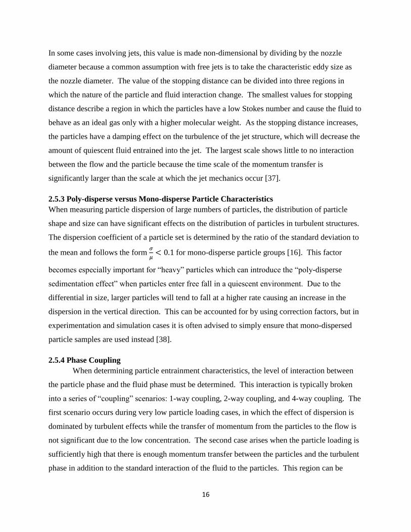
23

limited to a single particle for each meshed element on that surface, a Stochastic tracking

function was added. In this process, particles are staggered spatially in order to achieve a higher

utilization of the surface and allowing for a higher number of particles to be tracked without

significantly increasing the computational requirement. A sample of the particle injection

tracking scheme using the 1mm glass particles can be seen below in Figure 6. The particles fall

under the force of gravity from the injection surface, and are entrained into the flow before

exiting at the nozzle.

The particle interaction with the walls of the injection system was controlled using the “reflect”

boundary condition on all exterior faces of the mesh except those define in Figure 4. In doing so,

any particle collision with the walls will alter the trajectory of any particle according to its

coefficient of restitution. The values for the coefficients of restitution were determined though

simple experimentation by measuring the ratio of the initial height of a particle to the height after

one impact with a surface of material similar to that of the PVC pipe. This test showed that the

values for all sizes of glass particles were nearly identical at 0.65. The chrome steel was slightly

lower at 0.50, while the Zirconia and Zirconia-Silica were in between at 0.55 and .60

respectively. These values were passed into FLUENT as constant coefficients of restitution for

each case for both the normal and tangential components of the reflection behavior.

Figure 6: Sample Particle Injection Tracking (1mm glass) Color Coded by Particle

Residence Time (s)

24

3.2 Quiescent Environment (Wind Tunnel)

3.2.1 Wind Tunnel Geometry

In order to produce results usable as a baseline for future investigation, a controlled quiescent

environment was created using large panels of Plexiglas to create a wind tunnel measuring 4 feet

in width, 8 feet in height, and 16 feet in length with a 2 inch jet nozzle at one end and an open

pressure outlet at the opposing end. This was modeled in FLUENT using wall conditions for the

boundaries with the exception of the end wall which was modeled as a pressure outlet venting to

the atmosphere (i.e. zero gauge pressure). Upon initial simulations and experimental results, the

size of the control volume and the need for a fine mesh to effectively measure the domain

required a change in the geometry used.

Preliminary experimentation demonstrated that, for the particle sizes and densities tested, the

highest average distance traveled by entrained particles was approximately 54 inches (1.372 m)

for the 1.121 Zirconia-Silica particles. In order to allow a mesh with sufficiently small elements,

the overall length of the tunnel was shortened from 16 feet to 10 feet.

3.2.2 Wind Tunnel Meshing

Similar to the injection system, an “Advanced Sizing Function: Fixed” condition was used to

create the mesh for the wind tunnel. In this case, an additional face sizing feature was added to

the velocity inlet in order to provide a higher level of accuracy for both initialization purposes

and to allow for a higher accuracy for initial particle injection. Initial testing indicated that a

coarse mesh at the inlet provided significant error in the initial velocity in the core of the jet

structure. This error could propagate as the simulation ran, producing results that are unreliable.

As was the case with the injection system, a variety of mesh sizes were tested in order to test for

grid independence; the finest mesh tested contained 400,000 nodes and can be seen below in

Figure 7.

25

Figure 7: Wind Tunnel Mesh (Finest)

3.2.3 Wind Tunnel Particle Tracking

The Lagrangian tracking scheme was used again for this stage of the simulation using the same

sample of particles as discussed in section 3.1.3. As was the case with the injection system, the

particle volume fraction was calculated in order to determine the effect of phase coupling. In

order to determine the most conservative estimate of the volume fraction, only the volume of the

core jet structure (a canonical shape with an 11.8° angle and a height of 10 feet) was used to

determine the volume fraction. A sample, simulated flow field visualization of this structure can

be seen in Figure 8. In this figure, the fluid entrainment into the core structure can be seen as

well as the spreading angle. In this case the spreading half angle was measured along the initial

core structure, and was approximately 12°, agreeing well with the theoretical and experimental

studies on turbulent axisymmetric jets. In addition, the vector plot shows the characteristic

entrainment of fluid into the jet core causing the growth in the shear layer with relation to

distance from the nozzle.

26

Figure 8: Wind Tunnel Simulation Result Showing Jet Core Velocities (m/s)

Using this characteristic volume, the volume fraction for a loading of 100 particles (experimental

standard) of 5.995 mm glass produced a volume fraction on the order of 10-8

, placing it firmly

within the one-way coupling region.

27

Chapter 4: Initial Simulation and Experimentation

4.1 Impinging Jets in Confined Environments

One of the first investigations into turbulent jets and entrainment properties used a simple cube

with a velocity inlet centered on the top plane with outflows centered on the sides of the

geometry. The physical model can be seen below in Figure 9, where an added support structure

was constructed in order to provide stability to the flow source.

Figure 9: Impinged Jet Box Experiment The purpose of this experiment was to determine what effect (if any) particle size has on the

entrainment into a turbulent structure, in this case the impinging jet. As can be seen in the

figure, particles are loaded on the bottom surface of the control volume; note that in this figure a

test was being performed to simulate a large particle size fluidized bed while a normal set-up

would consist of only a single layer of particles. The model consisted of a 1 ft3 cube with 2 inch

diameter circular inlets centered as described.

The flow field was modeled using the Realizable k-ε turbulence model assuming a uniform

initial inlet velocity of 30 m/s (estimated based on air supply specifications and flow meter

measurements). The flow field was examined by looking at the center plane of the box, aligned

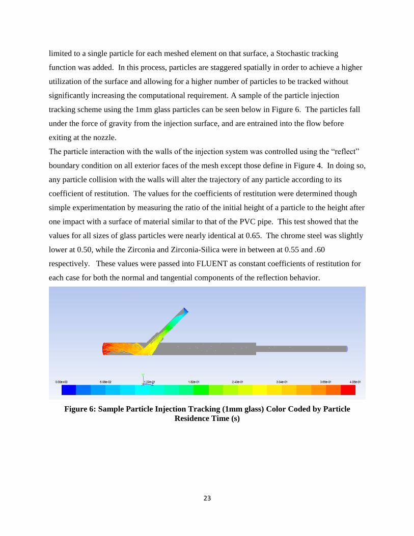
to show both of the outlets. This flow field can be seen below in Figure 10. As expected, the jet

28

impinges upon the bottom of the control volume, creating a symmetric flow pattern about the

central stagnation point. The recirculation from the bottom plane is the mechanism by which

particles are entrained into the flow and, depending on the trajectory of said particles, escape

through one of the centered outlets on the side of the box.

Figure 10: Box Experiment Center Plane Velocity Flow Field (m/s)

4.2 Particle Dispersion Simulation Results

Surface injections using different particle sizes were created on the bottom plane of the control

volume in order to test dispersion patterns of the particles in relation to their size. The primary

proof of concept particle used was standard industrial airsoft pellets with a diameter of 6mm and

a density of 1060 kg/m3. In this test, particles failed to entrain in the upward currents, and

instead were carried along the floor of the box to the four corners of the domain where stagnation

points developed. This same behavior was seen in the simulation using the Lagrangian tracking

scheme. In order to advance experimental runs, simulations were carried out using progressively

smaller particle diameters (holding density constant) in order to determine a minimum particle

size for entrainment to occur at the specified conditions.

29

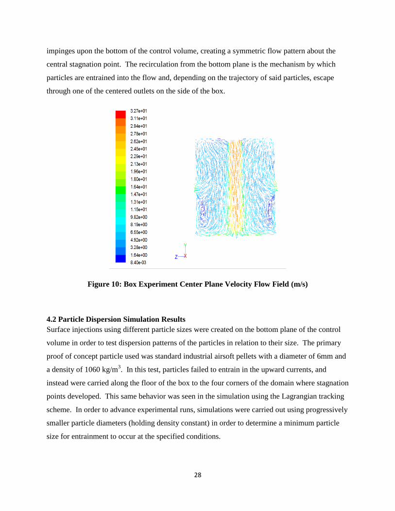
In order to measure the magnitude of entrainment, the percent evacuation of particles from the

control volume was calculated for each particle size. The primary concern with this method was

the manner in which FLUENT exports particle status as “escaped” (crossing one of the pressure

outlet boundaries) or “incomplete” (still within the control volume). In order to eliminate this

problem, for any cases which reported particles as “incomplete”, the number of time steps used

by the discrete phase model was increased by 10% and the particle tracking solution was run

again. This was done until no change in the number of particles marked as “incomplete” was

observed. With the number of particles marked as “incomplete” not changing, the position of

these particles was inspected using a particle tracking display. In each case evaluated, the

“incomplete” particles had become trapped in circulating loops or at stagnation points.

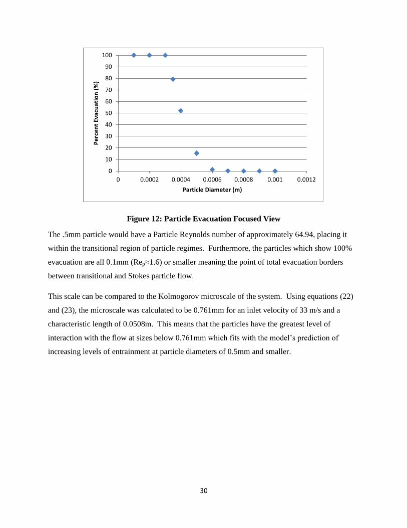
With the final fate of each particle determined for various sizes, a plot was generated to compare

the particle size to the percent evacuation from the chamber which can be seen in Figure 11.

Figure 11: Box Experiment Particle Size Percent Evacuation Relationship

This plot shows a rapid change in the magnitude of entrainment experienced by particles based

on particle size with the first particle of significant evacuation being 0.5mm in diameter. A more

detailed view of the change on a linear scale can be seen in Figure 12.

0

10

20

30

40

50

60

70

80

90

100

0.0000001 0.000001 0.00001 0.0001 0.001 0.01

Pe

rce

nt

Evac

uat

ion

(%

)

Particle Diameter (m)

30

Figure 12: Particle Evacuation Focused View

The .5mm particle would have a Particle Reynolds number of approximately 64.94, placing it

within the transitional region of particle regimes. Furthermore, the particles which show 100%

evacuation are all 0.1mm (Rep≈1.6) or smaller meaning the point of total evacuation borders

between transitional and Stokes particle flow.

This scale can be compared to the Kolmogorov microscale of the system. Using equations (22)

and (23), the microscale was calculated to be 0.761mm for an inlet velocity of 33 m/s and a

characteristic length of 0.0508m. This means that the particles have the greatest level of

interaction with the flow at sizes below 0.761mm which fits with the model’s prediction of

increasing levels of entrainment at particle diameters of 0.5mm and smaller.

0

10

20

30

40

50

60

70

80

90

100

0 0.0002 0.0004 0.0006 0.0008 0.001 0.0012

Pe

rce

nt

Evac

uat

ion

(%

)

Particle Diameter (m)

31

Chapter 5: Simulation Analysis In order to ensure the highest quality results from the simulations discussed series of grid

independence studies were conducted. Using the fixed advanced sizing function, the cell size

was lowered in order to double the number of nodes used in the simulation.

5.1 Injection System Grid Independence

Since the injection system focused on producing a variety of results for implementation in later

simulations, an effective grid independence study was required in order to ensure that the results

were accurate. This was accomplished by initially creating a series of 4 meshes of increasing

number of nodes starting with 100,000 nodes. This simulation was evaluated for flow

characteristics including overall pipe centerline velocity and nozzle velocity profile. Using the

fixed sizing function, the average cell size was reduced by a factor of 2 (approximately doubling

the number of nodes) and the simulation was run again. This process was repeated two more

times to produce meshes of 400,000 nodes and 800,000 nodes. It is important to note that the

simulating utilizing the 800,000 node mesh was never carried to completion due to

computational limitations producing an estimated completion time on the order of 30+ days.

Using the first three mesh sizes, the flow characteristics were compared in order to determine the

effect of any discretization error from mesh coarseness. The first comparison was of the

centerline velocity of the injection system. The overlaid centerline velocities of each case can be

seen in Figure 13. The plot shows that for the coarsest mesh case, there are significant

fluctuations in the velocity at the change in pipe diameter and around the point where the 45°

injection tube joins the geometry. By comparison, the medium and fine meshes show little

fluctuations and are nearly identical.

32

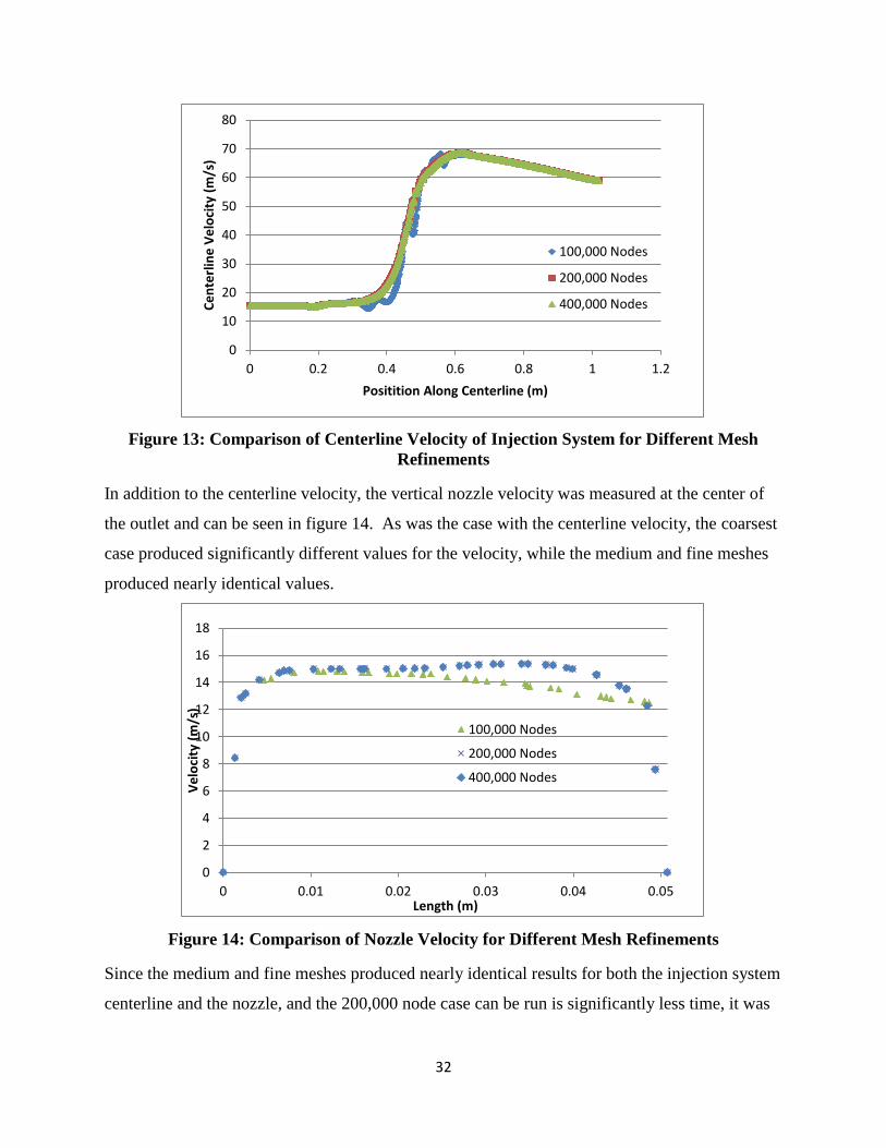
Figure 13: Comparison of Centerline Velocity of Injection System for Different Mesh

Refinements

In addition to the centerline velocity, the vertical nozzle velocity was measured at the center of

the outlet and can be seen in figure 14. As was the case with the centerline velocity, the coarsest

case produced significantly different values for the velocity, while the medium and fine meshes

produced nearly identical values.

Figure 14: Comparison of Nozzle Velocity for Different Mesh Refinements

Since the medium and fine meshes produced nearly identical results for both the injection system

centerline and the nozzle, and the 200,000 node case can be run is significantly less time, it was

0

10

20

30

40

50

60

70

80

0 0.2 0.4 0.6 0.8 1 1.2

Ce

nte

rlin

e V

elo

city

(m

/s)

Positition Along Centerline (m)

100,000 Nodes

200,000 Nodes

400,000 Nodes

0

2

4

6

8

10

12

14

16

18

0 0.01 0.02 0.03 0.04 0.05

Ve

loci

ty (

m/s

)

Length (m)

100,000 Nodes

200,000 Nodes

400,000 Nodes

33

selected as the mesh to carry out further simulations involving the particle injections to provide

additional validation data.

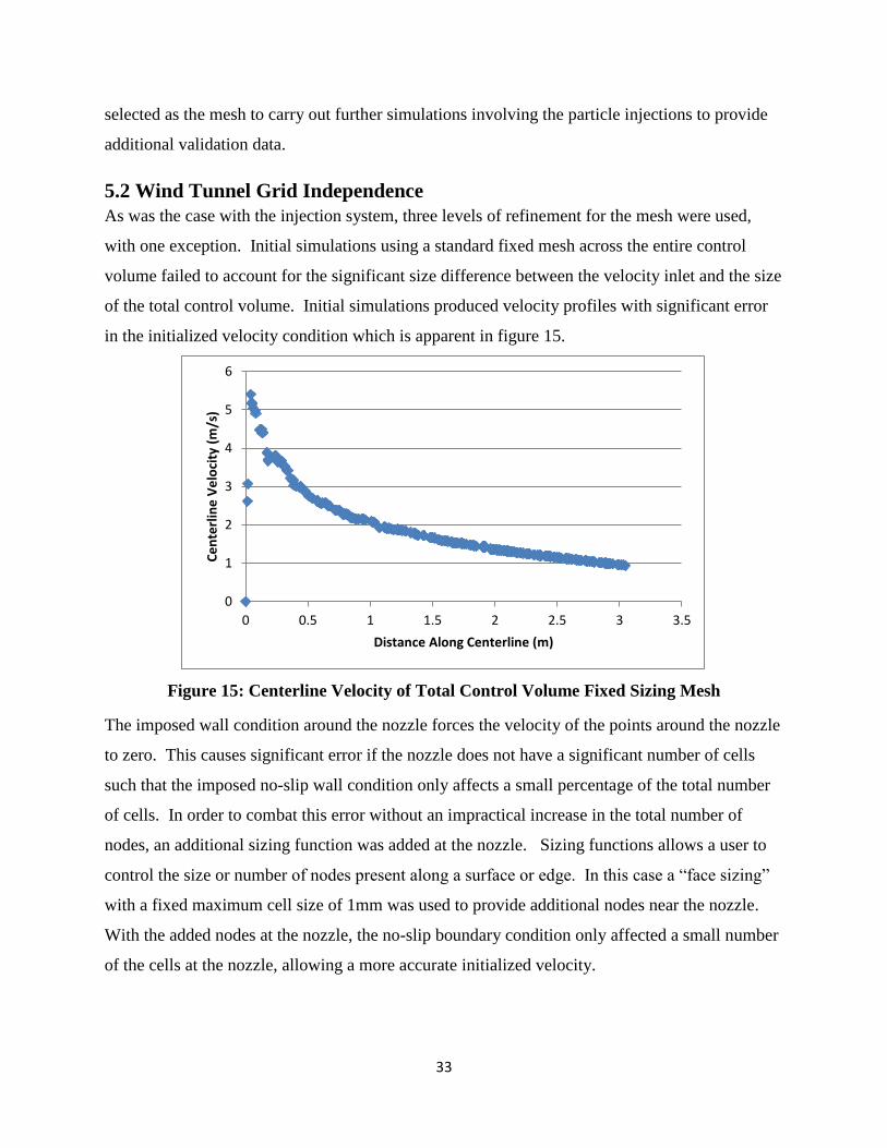
5.2 Wind Tunnel Grid Independence

As was the case with the injection system, three levels of refinement for the mesh were used,

with one exception. Initial simulations using a standard fixed mesh across the entire control

volume failed to account for the significant size difference between the velocity inlet and the size

of the total control volume. Initial simulations produced velocity profiles with significant error

in the initialized velocity condition which is apparent in figure 15.

Figure 15: Centerline Velocity of Total Control Volume Fixed Sizing Mesh

The imposed wall condition around the nozzle forces the velocity of the points around the nozzle

to zero. This causes significant error if the nozzle does not have a significant number of cells

such that the imposed no-slip wall condition only affects a small percentage of the total number

of cells. In order to combat this error without an impractical increase in the total number of

nodes, an additional sizing function was added at the nozzle. Sizing functions allows a user to

control the size or number of nodes present along a surface or edge. In this case a “face sizing”

with a fixed maximum cell size of 1mm was used to provide additional nodes near the nozzle.

With the added nodes at the nozzle, the no-slip boundary condition only affected a small number

of the cells at the nozzle, allowing a more accurate initialized velocity.

0

1

2

3

4

5

6

0 0.5 1 1.5 2 2.5 3 3.5

Ce

nte

rlin

e V

elo

city

(m

/s)

Distance Along Centerline (m)

34

The same meshing technique as the injection system was used to create a series of progressively

finer meshes for the wind tunnel containing approximately 100,000 nodes, 200,000 nodes, and

400,000 nodes. The centerline velocities for these three cases can be seen in more detail in

figure 16.

Figure 16: Comparison of Tunnel jet Centerline Velocities for Different Mesh Refinements

The figure shows a significant error for the coarsest mesh tested. In this case, the elements are

too large to effectively calculate the dissipation leading to a higher predicted velocity. In

addition, due to the large control volume, with a smaller region of high fluctuations, grid

adaptations were investigated as a potential solution to create a mesh of sufficient refinement for

the jet core. Attempts to produce a mesh of sufficient refinement within the jet core did not

appreciably increase the accuracy of the model or decrease the time and computational need. In

future simulations, if significantly higher jet velocities are required, FLUENT possesses the

ability to refine meshes based on gradients which could be used to produce targeted refinements

at points within the shear layer of the jet without increasing the total number of cells to an

unreasonable level.

0

2

4

6

8

10

12

14

16

0 0.5 1 1.5 2 2.5 3 3.5

Ce

nte

rlin

e V

elo

city

(m

/s)

Distance Along Centerline (m)

100,000 Nodes

200,000 Nodes

400,000 Nodes

35

Chapter 6: Injection System Simulation Results This section details the results of the computational simulation for both the injection system as

well as the quiescent environment. The results evaluated include flow field evaluation in relation

to a theoretical solution and particle dispersion patterns.

6.1 Injection System Flow Field Results

The first result gathered from the particle injection system was a general flow profile set at the

center plane of the geometry. The goal of generating this profile was in part to see the

significance of the change in pipe diameter upstream from the actual injection system. As can be

seen below in Figure 17, the fluid behaves similar to the jet mechanics present in the larger

quiescent environment and quickly disperses into standard pipe flow. This view can also be used

to determine the flow development in relation to the pipe length. The velocity vector plot shows

fairly constant velocity well before the injection port and continues after the port to the nozzle.

Figure 17: Injection System Center Plane Velocity Profile (m/s)

In order to determine how developed the pipe flow was at the nozzle where it ejects into a

quiescent environment, a velocity profile was generated for the nozzle (Figure 18). In this case,

0 m indicates the lowest point in the y direction of the nozzle (the lower left point in Figure 17).

36

Figure 18: Injection System Nozzle Velocity Where x=0 corresponds to the lowest point

along the centerline of the nozzle

The nozzle velocity shows a near constant velocity across the majority of the domain with sharp

drops in velocity approaching the walls in keeping with the no slip boundary condition imposed

on the walls of the domain. This indicates that the assumption of a constant velocity at the inlet

of the quiescent environment was reasonable.

6.2 Injection System Particle Behavior

Since the primary focus of this research is the dispersion and entrainment characteristics of

particles in a standard free jet, the effect the particle injection system has on particle behavior

leading into the quiescent environment was examined. The first parameter measured was the

mean velocity of particles crossing the ejection nozzle. The velocity determined using the

Lagrangian tracking scheme can be seen below in Table 3.

Table 3: Particle Injection Velocity at Nozzle

Material Type: Glass Glass Glass Glass Chrome

Steel

Zirconia-

Silica Zirconia

Measured Mean Particle

Diameter (mm): 5.995 3.646 2.602 1.168 2.383 1.121 1.072

Average Nozzle Velocity

(m/s) 1.70 1.99 2.25 2.58 1.61 2.77 2.43

Nozzle Velocity Standard

Deviation (m/s) .1070 .0876 .0860 .1376 .1216 .1094 .0938

0

2

4

6

8

10

12

14

16

18

0 0.01 0.02 0.03 0.04 0.05

Ve

loci

ty (

m/s

)

Nozzle Height (m)

37

The simulation of the glass particles showed that particle size played a significant role in the

velocity of the particle at the nozzle. As the particle size decreases, the velocity at which the

particle leaves the control volume increases due to the added interaction between the particle and

the fluid phase. This can be seen in detail by comparing the particle tracking paths displayed

below in Figure 19.

Figure 19: Particle Tracking Displays for 5.99 mm (Top) and 1.168 mm Glass (Bottom)

Color Coded by Particle Residence Time

The tracking schemes show two different types of dominant behavior at different points within

the domain. When the smaller particles fall from the injection surface, the higher level of

interaction with the flow causes the location of the first bounce to become more determinative of

the particle location and distribution across the nozzle as the velocity of the particles quickly

increases carrying the particle out of the domain. This can be seen by the fact that the majority

of the 1.16 mm glass particles bounce once and are then carried out of the domain by the flow.

In contrast, while the larger particles do still have bouncing causing some of the behavior, the

flow field is insufficiently strong to overcome all of the inertial effects of the particles as it was

with the smaller and lighter particles. This creates a particle concentration bias across the nozzle

38

where the mean starting particle position deviates from the center of the jet. This will be

discussed in additional detail in the following section. The intermediate sizes (2.60 mm and 3.64

mm) show behavior with aspects of both the 1.16 mm and 5.99 mm, where the 2.60 mm particles

show a similar limited bouncing behavior due to a higher level of interaction with the flow. In

this case, however, the particles have sufficient inertia as to change the final location of the

particles at the nozzle. The 3.64 mm particles show a very similar behavior to the 5.99 mm case,

sharing the more randomly spread particle dispersion.

Figure 20: Particle Tracking Displays for 3.64 mm (Top) and 2.60 mm Glass (Bottom)

Color Coded by Particle Residence Time

In order to compare the effect density has on the particle dispersion within the injection system,

the 1.168 mm glass, 1.121 mm Zirconia Silica, and 1.071 mm Zirconia particle tracks were

compared. The particle dispersion tracking paths for the Zirconia-Silica and Zirconia can be

seen in Figure 21.

39

Figure 21: Particle Tracking Displays for 1.071 mm Zirconia (Top) and 1.121 mm

Zirconia-Silica (Bottom) Color Coded by Particle Residence Time

The Zirconia-Silica particle which is approximately 50% more dense than glass has similar

behavior to the glass. Once the particle exits the injection tube, it falls under the force of gravity

until it bounces off the bottom surface and is then entrained in the flow which causes a bias to

the top half of the pipe due to the distance of the nozzle from the injection port. In contrast, the

1.071 Zirconia particles bounce more than once within the pipe which causes a greater dispersion

across the inlet, however, due to the location of the nozzle there is still a partial bias toward the

top half of the nozzle.

For comparison purposes, histograms of the particle location across the nozzle can be seen for

each case below. Special attention should be paid to the Glass 1.168 mm and Zirconia-Silica

1.121 mm since they have the highest dispersion bias toward one half of the pipe. In addition,

the Zirconia 1.072 mm particles also have a slight bias to the top half of the duct and the Glass

3.646mm has a slight bias to the lower half of the nozzle.

40

Figure 22: Histograms of Dispersion of Tested Particles Across Nozzle

-0.03 -0.02 -0.01 0 0.01 0.02 0.030

5

10

15

20

25

height (m)

Part

icle

Count

Chrome Steel (2.383mm)

-0.03 -0.02 -0.01 0 0.01 0.02 0.030

5

10

15

20

25

30

35

height (m)

Part

icle

Count

Glass (1.168mm)

-0.03 -0.02 -0.01 0 0.01 0.02 0.030

5

10

15

20

25

height (m)

Part

icle

Count

Glass (2.602mm)

-0.03 -0.02 -0.01 0 0.01 0.02 0.030

5

10

15

20

25

30

height (m)

Part

icle

Count

Glass (3.646mm)

-0.03 -0.02 -0.01 0 0.01 0.02 0.030

5

10

15

20

25

height (m)

Part

icle

Count

Glass (5.995mm)

-0.03 -0.02 -0.01 0 0.01 0.02 0.030

5

10

15

20

25

30

height (m)

Part

icle

Count

Zirconia (1.072mm)

-0.03 -0.02 -0.01 0 0.01 0.02 0.030

5

10

15

20

25

30

35

height (m)

Part

icle

Count

Zirconia-Silica (1.121mm)

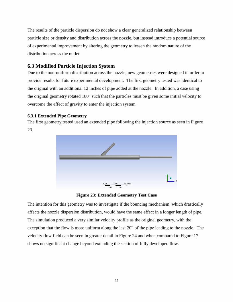
41

The results of the particle dispersion do not show a clear generalized relationship between

particle size or density and distribution across the nozzle, but instead introduce a potential source

of experimental improvement by altering the geometry to lessen the random nature of the

distribution across the outlet.

6.3 Modified Particle Injection System

Due to the non-uniform distribution across the nozzle, new geometries were designed in order to

provide results for future experimental development. The first geometry tested was identical to

the original with an additional 12 inches of pipe added at the nozzle. In addition, a case using

the original geometry rotated 180° such that the particles must be given some initial velocity to

overcome the effect of gravity to enter the injection system

6.3.1 Extended Pipe Geometry

The first geometry tested used an extended pipe following the injection source as seen in Figure

23.

Figure 23: Extended Geometry Test Case

The intention for this geometry was to investigate if the bouncing mechanism, which drastically

affects the nozzle dispersion distribution, would have the same effect in a longer length of pipe.

The simulation produced a very similar velocity profile as the original geometry, with the

exception that the flow is more uniform along the last 20” of the pipe leading to the nozzle. The

velocity flow field can be seen in greater detail in Figure 24 and when compared to Figure 17

shows no significant change beyond extending the section of fully developed flow.

42

Figure 24: Extended Geometry Velocity Flow Field

The nozzle velocity profile for the extended geometry was compared to the original geometry in

order to determine what nozzle effect, if any, the added length would have on the velocity profile

that enters the quiescent environment. The profiles for each geometry can be seen in Figure 25.

The velocity profile shares the same blunted profile characteristic of fully developed flow which

indicates that the added geometry has little to no effect on the flow and instead can be evaluated

for a particle dispersion effect.

Figure 25: Comparison of Extended Geometry Nozzle Velocity

0

2

4

6

8

10

12

14

16

18

0 0.01 0.02 0.03 0.04 0.05

Ve

loci

ty (

m/s

)

Length (m)

OriginalGeometry

ExtendedGeometry

43

Once the nozzle velocities for each geometry were compared, the particle tracking for each of the

cases tested was simulated using the same Lagrangian tracking scheme. The first comparison for

the new geometry was the average particle velocity at the nozzle which can be seen in Table 4.

Table 4: Extended Geometry Particle Velocities

Material Type: Glass Glass Glass Glass Chrome

Steel

Zirconia-

Silica Zirconia

Measured Mean Particle

Diameter (mm): 5.995 3.646 2.602 1.168 2.383 1.121 1.072

Average Nozzle Velocity

(m/s) 2.24 3.00 3.11 4.99 2.11 3.88 3.39

Nozzle Velocity Standard

Deviation (m/s) .0945 .119 .099 .113 .093 .1189 .1055

Percent Change from

Original (%) 31.7 50.7 38.2 57.4 31.1 40.1 39.5

The particle velocities are consistently higher for the extended pipe length with minor changes

for the standard deviation across all particle sizes and materials. The increase in velocity can be

attributed to the additional time required for the particles to reach the nozzle. The additional

length allows the particles to become more entrained with the flow. This is particularly

important for the smaller particles which had a significant increase in velocity. This could

complicate experimental procedures if the additional velocity is not accounted for.

In addition, the particle distribution across the nozzle is significantly affected by the increase in

pipe length for certain particle sizes and densities. Figure 26 demonstrates that the additional

pipe length produces a particle distribution across the nozzle with a significantly more Gaussian

distribution for the cases which showed the greatest bias in the standard configuration. The

distributions for the new geometry can be seen in detail in Figure 27 as a particle tracking

scheme.

44

Figure 26: Particle Distribution Across Nozzle

The distribution for all of these cases was shown to be significantly more Gaussian for these

particles within the new geometry. The remaining particle sizes and densities showed less

significant changes in distribution, however, all cases did tend toward a more Gaussian

distribution on the whole. The behavior of the three distributions with the most significant

changes is easier to see when comparing the Lagrangian particle history data.

-0.03 -0.02 -0.01 0 0.01 0.02 0.030

5

10

15

20

25

30

35

40

45

50

height (m)

Part

icle

Count

Glass (1.168mm)

-0.03 -0.02 -0.01 0 0.01 0.02 0.030

10

20

30

40

50

60

height (m)

Part

icle

Count

Zirconia-Silica (1.121mm)

-0.03 -0.02 -0.01 0 0.01 0.02 0.030

5

10

15

20

25

30

35

40

45

50

height (m)

Part

icle

Count

Glass (3.646mm)

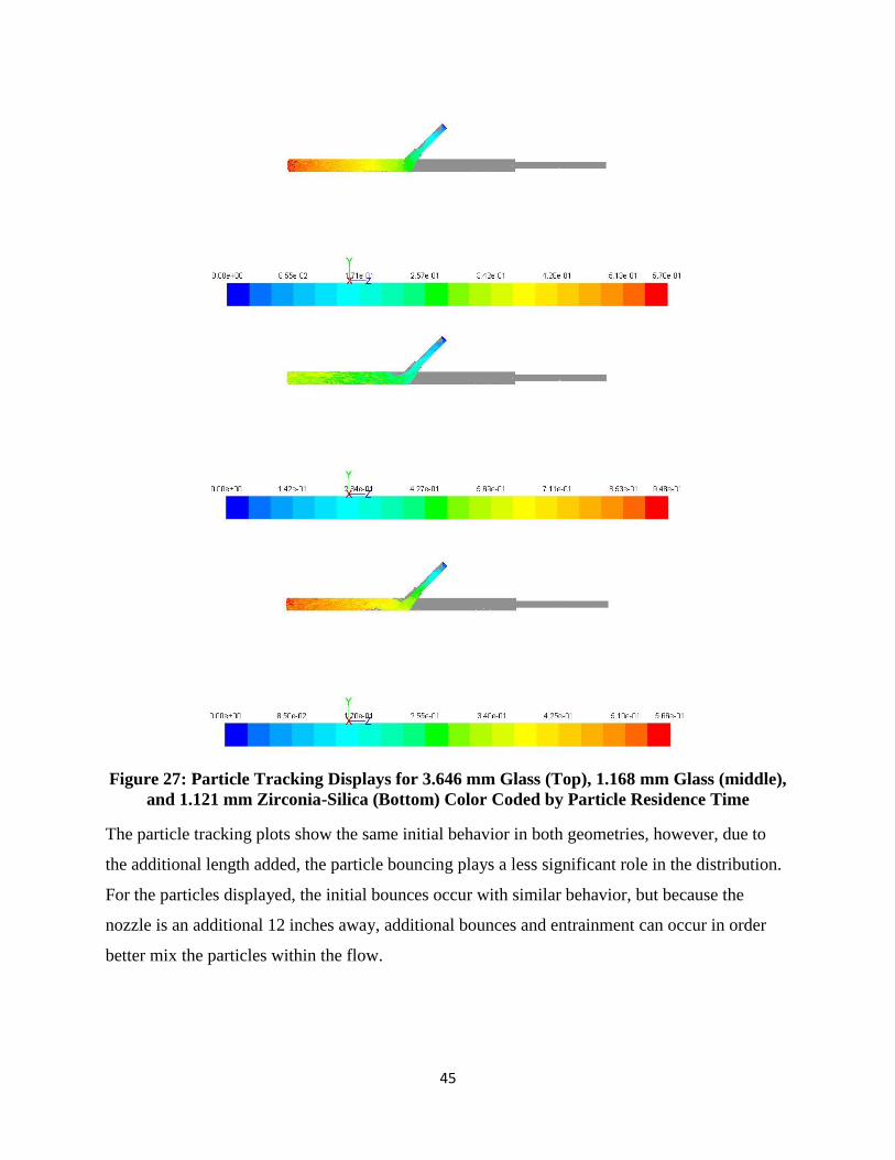
45

Figure 27: Particle Tracking Displays for 3.646 mm Glass (Top), 1.168 mm Glass (middle),

and 1.121 mm Zirconia-Silica (Bottom) Color Coded by Particle Residence Time

The particle tracking plots show the same initial behavior in both geometries, however, due to

the additional length added, the particle bouncing plays a less significant role in the distribution.

For the particles displayed, the initial bounces occur with similar behavior, but because the

nozzle is an additional 12 inches away, additional bounces and entrainment can occur in order

better mix the particles within the flow.

46

Given the improvement in particle distribution, this change in geometry is most likely the

simplest alteration to the experimental geometry that could provide more reliable and consistent

results for future tests.

6.3.2 Modified Operating Conditions

An additional method to improve the quality of particle distribution in the injection system was

to alter the operating condition and orientation of the system as a whole. A common practice in

testing particle dispersion is to use acoustic forcing of particles to orient them in a particular

structure. That idea inspired a method in an attempt to limit the effect that initial particle

bouncing has on the system. In this configuration, the injection system is rotated 180° such that

particles must be forced up into the system with some initial velocity to overcome the

gravitational force instead of letting gravity pull the particles into the pipe.

This method creates some complications in selecting an initial velocity for the particle injections.

For that reason, the simulations provide two functions: determining an initial velocity capable of

injecting particles into the flow and determining what effect this method has on the particle

distribution across the nozzle. The initial velocities for the particle injections were individually

iteratively derived based on an initial estimate for the particles to take the same amount of time

to reach the pipe flow using the standard equations of motion. These basic calculations produce

a velocity of 2.048 m/s normal to the injection surface (at a 45° angle to the pipe flow). The

iteration process produced the following velocity/particle combinations which produced the most

normal particle distribution can be seen in Table 5 below.

Table 5: Initial Particle Velocity for Modified Injection System

Material Type: Glass Glass Glass Glass Chrome

Steel

Zirconia-

Silica Zirconia

Measured Mean Particle

Diameter (mm): 5.995 3.646 2.602 1.168 2.383 1.121 1.072

Particle Injection

Velocity: Normal to

Surface (m/s)

2.26 2.47 2.54 2.54 2.26 2.33 2.68

47

The particle distribution can be seen for the particles tested below in Figure 28. Compared to the

original geometry with gravity fed injection, the distribution using an initial velocity injection

follows a significantly more normal distribution across all cases. The particles produced very

similar velocities and standard deviations as the original geometry (the values can be seen in

Table 6), which indicates that the initial velocity and injection again the force of gravity has a

less significant effect on the velocity of particles leaving the nozzle. If the geometry tested

cannot be easily altered, simply inverting the injection system and designing a secondary system

to inject particles could be a viable method to produce more normal distributions.

Table 6: Particle Nozzle Velocity for Initial Velocity Condition

Material Type: Glass Glass Glass Glass Chrome

Steel

Zirconia-

Silica Zirconia

Measured Mean Particle

Diameter (mm): 5.995 3.646 2.602 1.168 2.383 1.121 1.072

Average Nozzle Velocity

(m/s) 1.57 1.95 2.21 3.07 1.48 2.64 2.43

Nozzle Velocity Standard

Deviation (m/s) .118 .125 .125 .161 .118 .159 .136

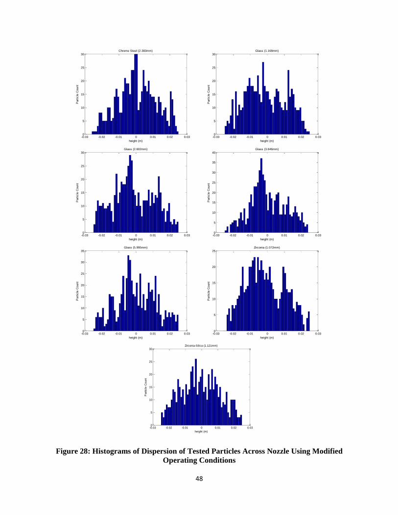
48

Figure 28: Histograms of Dispersion of Tested Particles Across Nozzle Using Modified

Operating Conditions

-0.03 -0.02 -0.01 0 0.01 0.02 0.030

5

10

15

20

25

30

height (m)

Part

icle

Count

Chrome Steel (2.383mm)

-0.03 -0.02 -0.01 0 0.01 0.02 0.030

5

10

15

20

25

30

height (m)

Part

icle

Count

Glass (1.168mm)

-0.03 -0.02 -0.01 0 0.01 0.02 0.030

5

10

15

20

25

30

height (m)

Part

icle

Count

Glass (2.602mm)

-0.03 -0.02 -0.01 0 0.01 0.02 0.030

5

10

15

20

25

30

35

40

height (m)

Part

icle

Count

Glass (3.646mm)

-0.03 -0.02 -0.01 0 0.01 0.02 0.030

5

10

15

20

25

30

35

height (m)

Part

icle

Count

Glass (5.995mm)

-0.03 -0.02 -0.01 0 0.01 0.02 0.030

5

10

15

20

25

height (m)

Part

icle

Count

Zirconia (1.072mm)

-0.03 -0.02 -0.01 0 0.01 0.02 0.030

5

10

15

20

25

30

height (m)

Part

icle

Count

Zirconia-Silica (1.121mm)

49

Due to the limitations in collecting experimental data, the results of this simulation were used to

perform additional tests on the wind tunnel side of the simulation. The simulation results which

produced some non-zero velocities for particle exiting the injection system were used to better

predict the behavior of injected particles compared to stationary particle injections directly at the

nozzle of the system. In addition, the simulation which illustrated a heavily non-uniform particle

distribution across the nozzle was used to create secondary simulations which would test the

effect of discretizing the nozzle into regions where the effect of starting height in the nozzle

could be measured relative to particle dispersion.

50

Chapter 7: Wind Tunnel Results Initial experimental results as well as results from the simulation of the injection system revealed

the need to test two configurations of the wind tunnel for simulation. The experimental results

indicated a non-symmetric distribution of particles falling out of entrainment within the jet core.

It was speculated that this was due to an uneven particle distribution at the nozzle exit. For this

reason, a different inlet was created where the particle distribution could be weight to either the

top or bottom half of the nozzle and was tested along with the standard uniform distribution.

7.1 Simulation Flow Field Evaluation

The results of the simulation were first analyzed in relation to the flow field, and how close it

matched a theoretical case for an axisymmetric turbulent jet. This was accomplished by

comparing the centerline velocity of the simulation to a theoretical one using equation (1) where

Bu was taken to be 5.0. In this case, the simulation used a nozzle velocity of 14.29 m/s (the

average velocity of the fully developed flow measured using a Pitot tube anemometer). The

comparison of the centerline velocities can be seen in Figure 29 below. The defining difference

between the two cases is the slight over-estimation of the velocity at the beginning of the jet

core. This difference is less significant at points down stream.

Figure 29: Comparison of Theoretical and Simulated Jet Centerline Velocity

In addition to the centerline velocity comparison, the spreading angle of the jet simulation was

compared to experimental and theoretical studies on turbulent axisymmetric jets. As was shown

previously, the simulated spreading rate of the jet was approximately 12°, fitting well with the

0

2

4

6

8

10

12

14

16

0 0.5 1 1.5 2 2.5 3 3.5

Ce

nte

rlin

e V

elo

city

(m

/s)

Distance Along Centerline (m)

TheoreticalVelocitySimulationVelocity

51

theoretical result of 11.8°. Due to this agreement between the simulated and theoretical results,

the simulation was used to test particle dispersion for the cases mentioned in Chapter 6.

7.2 Particle Dispersion Patterns

The particle dispersion simulation was broken down into a variety of different cases in order to

test which aspects of the dispersion were a result of conditions unique to the experimental

apparatus. The first case was deemed a “static injection” where the particles would be injected

with zero initial velocity across the nozzle. This condition would be difficult to replicate

experimentally given the current set up. The second condition better reflected the experimental

results, wherein the particles were given initial velocities equal to the mean velocity calculated

from the simulation of the injection system.

The Stokes number for each case studied was calculated using equation (21) using the

characteristic velocity of the jet. The particles tested provide a wide range of values and can be

seen in Table 7.

Table 7: Calculated Stokes Numbers for Particles Tested Within the Jet Geometry

Material Type: Glass Glass Glass Glass Chrome

Steel

Zirconia-

Silica Zirconia

Measured Mean Particle

Diameter (mm): 5.995 3.646 2.602 1.168 2.383 1.121 1.072

Particle Stokes Number 251.71 93.09 47.42 9.55 125.72 13.02 17.71

While all of the cases studied are outside the Standard Stokes regime (St≈1), it is expected that

the particles will not act explicitly as tracers to the flow. However, the 1mm scale particles

could show signs of Stokes flow and show higher adherence to flow path lines with substantial

lag time.

In addition to the Stokes number for each particle case, the Kolmogorov scale was calculated to

provide another method of quantifying the interaction between the fluid flow and the particle

motion. Compared to the box experiment discussed in Chapter 4, the inlet velocity of this case is

significantly lower, which will cause the Kolmogorov scale to be smaller. For this case, the

turbulent kinetic energy dissipation rate (ε) was taken from the results of the flow simulation,

52

and was spatially averaged to be 50 m2/s

3. By using this value with equation 22, the

Kolmogorov scale was calculated to be 90 microns (.09 mm). Given that all particles sizes tested

are at least one order of magnitude greater than the Kolmogorov scale, long term entrainment

would not be expected for any case.

A sample particle tracking result for these two conditions can be seen in Figure 30 below. The

particle injections show drastic differences in both the magnitude of distance traveled by the

particles, as well as the distribution across the domain. The static injection shows a minimal

displacement for the particles, with a high level of dispersion. The dynamic injection shows the

opposite characteristics with a much higher displacement and a more compact distribution of

particles. This result is related in part to the low velocity of the fluid exiting the nozzle. In the

case of the static injection, the particles injected in the lower extreme of the nozzle tend to

simply fall with minimal change in velocity. For particles experiencing the higher velocities at

the center of the jet core, the displacement is more significant. By comparison, in the dynamic

injection, the particles already have sufficient forward momentum that the flow does not need to

transfer as much energy to cause significant displacements. This behavior was seen across all

particle sizes and materials, while the 1mm scale particles showed the largest difference in

displacement.

53

a)

b)

Figure 30: a) Particle Tracking Result for 1.168mm Glass Static Particle Injection Color

Coded by Particle Residence Time (s) b) Particle Tracking Result for 1.168mm Glass

Initial Velocity Particle Injection Color Coded by Particle Residence Time (s)

A variety of particle dispersion characteristics were compared between the simulation of the

dynamic particle injection and the experimental results. The first and simplest parameter tested

was average distance traveled into the quiescent environment for the various particle injections.

Table 8 shows that the simulation effectively predicted the displacement of the particles within 2

to 12% of the experimental results depending on the particle tested. The simulation produced the

least accurate results for the 1mm scale glass and zirconia-silica particles, with errors of 9.476%

and 11.568% respectively compared to the experimental results. This significant increase in

error is due to the result generated through simulation of the injection system where it was shown

54

that for the 1mm scale glass and zirconia-silica there was a significant distribution bias toward

the top half of the nozzle. More detail on this issue will be discussed in section 7.3. Beyond

these two cases, there is minimal information to develop a trend for the error between the

simulation and experimentation.

Table 8: Comparison of Experimental and Simulation Mean Particle Displacement

Material Type: Glass Glass Glass Glass Chrome

Steel

Zirconia-

Silica Zirconia

Measured Mean

Particle Diameter

(mm):

5.995 3.646 2.602 1.168 2.383 1.121 1.072

Experimental

Displacement (in) 29.7 37.465 43.527 63.724 23.784 53.776 44.451

Simulated

Displacement(m/s) 28.061 39.219 42.164 58.208 22.262 48.200 43.186

Percent Difference

(%) 5.841 4.682 3.232 9.476 6.837 11.568 2.929

In comparison, the standard deviation of the simulated particle displacement was higher for the

majority of the cases tested. A comparison of the standard deviations for each particle type can

be seen in Table 9 below. The only particle which had a smaller standard deviation was

1.168mm glass, while the 1.121mm Zirconia-Silica had the closest approximation. Previous

simulations designed to test the particle distribution across the nozzle of the injection system

presented a possible solution for the discrepancy between the two cases. Simulations of the

injection system illustrated there was a non-uniform distribution of particles across the nozzle,

while this simulation was carried out with a uniform distribution across the nozzle for all cases.

While this was done as an initial test of the accuracy of the simulation, it could provide some

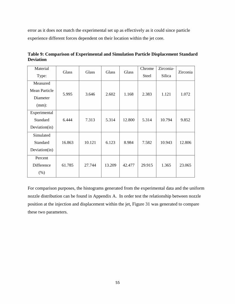
55

error as it does not match the experimental set up as effectively as it could since particle

experience different forces dependent on their location within the jet core.

Table 9: Comparison of Experimental and Simulation Particle Displacement Standard

Deviation

Material

Type: Glass Glass Glass Glass

Chrome

Steel

Zirconia-

Silica Zirconia

Measured

Mean Particle

Diameter

(mm):

5.995 3.646 2.602 1.168 2.383 1.121 1.072

Experimental

Standard

Deviation(in)

6.444 7.313 5.314 12.800 5.314 10.794 9.852

Simulated

Standard

Deviation(in)

16.863 10.121 6.123 8.984 7.582 10.943 12.806

Percent

Difference

(%)

61.785 27.744 13.209 42.477 29.915 1.365 23.065

For comparison purposes, the histograms generated from the experimental data and the uniform

nozzle distribution can be found in Appendix A. In order test the relationship between nozzle

position at the injection and displacement within the jet, Figure 31 was generated to compare

these two parameters.

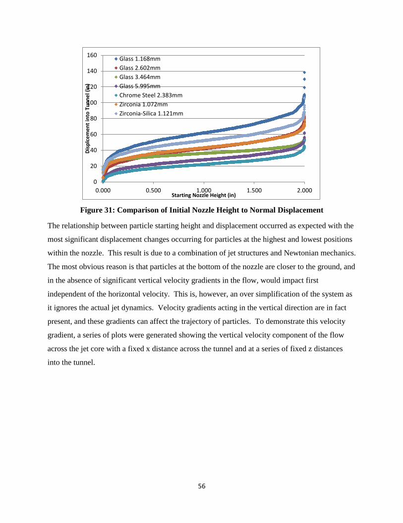
56

Figure 31: Comparison of Initial Nozzle Height to Normal Displacement

The relationship between particle starting height and displacement occurred as expected with the

most significant displacement changes occurring for particles at the highest and lowest positions

within the nozzle. This result is due to a combination of jet structures and Newtonian mechanics.

The most obvious reason is that particles at the bottom of the nozzle are closer to the ground, and

in the absence of significant vertical velocity gradients in the flow, would impact first

independent of the horizontal velocity. This is, however, an over simplification of the system as

it ignores the actual jet dynamics. Velocity gradients acting in the vertical direction are in fact

present, and these gradients can affect the trajectory of particles. To demonstrate this velocity

gradient, a series of plots were generated showing the vertical velocity component of the flow

across the jet core with a fixed x distance across the tunnel and at a series of fixed z distances

into the tunnel.

0

20

40

60

80

100

120

140

160

0.000 0.500 1.000 1.500 2.000

Dis

plc

em

en

t in

to T

un

ne

l (in

)

Starting Nozzle Height (in)

Glass 1.168mm

Glass 2.602mm

Glass 3.464mm

Glass 5.995mm

Chrome Steel 2.383mm

Zirconia 1.072mm

Zirconia-Silica 1.121mm

57

Figure 32: Comparison of Vertical Velocity Component at Various Positions along the Jet

Core

This plot shows the steady vertical velocity component and the fact that the transition from

negative to positive occurs around the centerline of the nozzle. For this reason, particles injected

on the top half of the nozzle are exposed to an additional lift component present in the flow field

caused by the entrainment of ambient air. This effect is especially important as the Stokes

number decreases in the system. As was previously stated, the Stokes number can be used to

measure how closely a particle will follow the flow path lines it is exposed to. Since Stokes

number is affected by particle size and particle density, it would be expected to see the 1mm

scale particles be the most affected by the velocity gradients in the flow. This result is seen in

both the experimental and simulated results for the 1mm scale glass and zirconia-silica, with a

lesser effect seen on the 2.602mm Glass and 1.072mm Zirconia, due in part to the higher density

of the Zirconia and larger diameter for the glass.

7.3 Particle Dispersion with Nozzle Bias

Experimental results indicated that in most cases, the particle distribution for some cases

produced a distribution with a non-zero Skewness, indicating that there is a larger tail on one

side of the distribution. The values of the Skewness calculated for the experimental trials can be

seen below in Table 10, along with those calculated from the simulated values.

-0.06

-0.04

-0.02

0

0.02

0.04

0.06

0.08

0.1

0.12

-0.15 -0.1 -0.05 0 0.05 0.1 0.15

Ve

rtic

al V

elo

city

Co

mp

on

en

t (m

/s)

Vertical (y) Distance From Centerline (m)

.5m

.7m

.9m

1.1m

1.3m

1.5m

1.7m

58

Table 10: Comparison of Skewness from Experimental and Simulated Results

Material Type: Glass Glass Glass Glass Chrome

Steel

Zirconia-

Silica Zirconia

Measured

Mean Particle

Diameter

(mm):

5.995 3.646 2.602 1.168 2.383 1.121 1.072

Experimental

Skewness 0.669 0.619 0.743 -0.788 0.918 0.442 0.540

Simulated

Skewness 0.033 0.005 0.065 0.100 0.001 0.043 -0.002

The comparison of the experimental versus simulated condition shows that the simulation

produced results that are significantly more Gaussian compared to the experiment. This is due in

part to the assumptions made when creating the simulation. For comparison purposes, the

histograms for both sets of data can be found in Appendix A. The primary difference is in the

particle injection distribution, where the simulation used a uniform distribution across the nozzle.

This was shown to be a faulty assumption based on both inspections during experimentation and

simulations of the injection system. The simulation of the injection system showed that in each

case, there was a bias to one half of the nozzle height. It is important to note that there could

also be a bias to the left or right half of the nozzle, but lack of experimental results for

comparison led to it not being evaluated.

In an attempt to better match the experimental results, a new simulated geometry was created

with the nozzle split into two equal area inlets representing the top and bottom halves of the

nozzle. When creating particle injections, this allowed use of the random walk model to produce

additional particle tracks across the top or bottom surface in order to create distributions which

better matched the results from the simulation of the injection system. Simulations of the

injection system showed the greatest disparity in distribution into the tunnel for the 1mm scale

glass and Zirconia-Silica and a lesser disparity for the case of the 3.646mm glass. Since these

three particle cases showed the most significant nozzle bias and overall high error in the

predicted displacement of the particles, they were the initial test cases to determine the effect of

the new weighting. The first case evaluated was the 1.168mm glass which showed the highest

59

nozzle bias with a large majority of particles (~90%) entering the tunnel from the top half of the

nozzle. The bias factor used was initially estimated from the results of the injection system

simulation, and then changed incrementally until the most accurate results were produced. The

bias factor for this case is defined as the percentage of the total number of injected particles

traveling through one half of the nozzle. The bias factors that were used for these cases were

90% (top half), 70% (top half), and 67% (bottom half) for the 1.168mm glass, 1.121mm

Zirconia-Silica, and 3.646mm glass respectively. This produced a new set of distributions which

can be seen in greater detail in Figure 33:

Figure 33: Distributions for Nozzle Bias Cases of Glass 1.168mm, Glass 3.646mm, and

Zirconia-Silica 1.121mm

As was the case with the uniform distribution of particles into the tunnel, the particle distribution

follows a standard Gaussian profile with an augmented mean from the original case. For the

biases used, the new mean more closely matches the experimental results presented in Table 11.

0 20 40 60 80 100 120 140 160 1800

100

200

300

400

500

600

700

800

900

1000

Displacement (in)

Part

icle

Count

Glass (1.168mm) Simulated

0 20 40 60 80 100 120 140 160 1800

50

100

150

200

250

300

350

400

450

500

Displacement (in)

Part

icle

Count

Glass (3.646mm) Simulated

0 20 40 60 80 100 120 140 160 1800

50

100

150

200

250

300

350

400

450

500

Displacement (in)

Part

icle

Count

Zirconia-Silica (1.121mm) Simulated

60

Table 11: Comparison of Experimental and Simulation Mean Particle Displacement Using

Nozzle Bias

Material Type: Glass Glass Zirconia-

Silica

Measured Mean

Particle Diameter

(mm):

3.646 1.168 1.121

Experimental

Displacement (in) 37.465 63.724 53.776

Simulated

Displacement(m/s) 37.514 64.049 53.080

Percent Difference

(%) 1.301 0.510 1.311

The added bias factor in the particle count significantly improved the simulated displacement for

these three cases, making them the closest matches to the experimental results. This indicates

that the model is most effective at simulating the dispersion of particles with a smaller Stokes

number compared to predicting the trajectories of larger and or heavier particles. This is

partially related to the particles with a higher Stokes number following a more standard

rectilinear motion trajectory, with minimal interaction with the flow. For that reason, the particle

displacement and distribution would be more significantly affected by the initial position and

velocity of the particles upon entering the control volume, propagating any discrepancies in the

injection system simulation into the wind tunnel simulation.

61

Chapter 8: Discussion and Conclusions It is clear from both the experimental and simulated results that both particle density and size

have significant impacts on entrainment properties within turbulent structures. By comparing the

cases of the constant density/variable size (glass) case and the constant size/variable density

(glass, Zirconia-Silica, Zirconia) it can be easily seen that particle entrainment is dependent on

both properties as expected. With the constant density case, the glass particles showed a

significantly non-linear relation to displacement for both the experimental and simulated results.

This is reasonable as this change affects multiple characteristic forces acting on the particles

including gravity, drag, and lift as well as the nature of the particle’s interaction with the flow

field. In addition, figure 34 shows that the experimental and simulated displacement for the

particle have the closest match to a particle undergoing standard ballistic motion as the diameter

of the particle increases.

Figure 34: Comparison of Particle Size to Mean Particle Displacement for Various Sizes of

Fixed Density (1060 kg/m3) Glass Particles

In addition to comparing the constant density case, the 1mm scale particles with variable

densities were also plotted to show the relationship between particle mass and displacement.

The outcome was again as expected, showing that particles with higher mass would fall faster

within the system as their inertia would mean interaction with the flow would not significantly

alter their trajectory for particles with very high masses. This was especially the case with the

0

10

20

30

40

50

60

70

0 0.001 0.002 0.003 0.004 0.005 0.006 0.007

Me

an D

isp

lace

me

nt

(in

)

Particle Size (m)

Experimental Displacement

Simulated Displacement

Ballistic Trajectory

62

chrome steel particles (experimental value is only 2.1% greater than ballistic displacement).

Even though the particles were relatively small in size (2.383 mm) the high density caused the

particles to follow a more standard ballistic trajectory out of the nozzle.

Figure 35: Comparison of Particle Displacement for Particles of Constant Size (1mm) and

Variable Density/Mass

Within the turbulent jet, the particle dispersion pattern across the lower surface of the quiescent

environment followed a Gaussian distribution for all particle cases tested independent of any

nozzle bias used. When comparing the particle displacement as a function of the starting nozzle

position, it was seen that the displacement in line with the jet was more significant for particles

away from the centerline as seen in Figure 31, where the lighter and smaller particles were the

most significantly affected by starting nozzle position. The behavior of particles at the extreme

top and bottom of the nozzle at the injection are interesting in that they are exposed to different

flow characteristics. Particles at the top of the nozzle would be expected to have the greatest

displacement by virtue of the fact that, with constant flow velocity gradients, they would be in

the air longer. However, this is only part of the issue. As was shown in Figure 32, the top half

of the jet core contains a vertical velocity component compared to the lower half of the core

which contains a downward velocity component. It must be noted that for this experiment and

simulation, the particle distribution showed significant dependence on the initial velocity and

position of the particles injected into the jet core.

0

10

20

30

40

50

60

70

0.00E+00 1.00E-06 2.00E-06 3.00E-06 4.00E-06

Me

an P

arti

cle

Dis

pla

cem

en

t (i

n)

Particle Mass (kg)

Experimental Displacement

Simulated Displacement

Ballistic Trajectory

63

In conclusion, the particle dispersion from a turbulent, axisymmetric round jet is predicted to

follow a standard Gaussian distribution following their falling out of entrainment within the jet

core. The model presented here has a significantly better ability to match particle displacement

behavior for cases in which the Stokes number of the system is lower (however in this case is

still considered non-Stokesian) as this case produced particle trajectories which better mimic the

flow characteristics. When comparing the simulated distributions to the experimental

distributions, the clear difference is in the Skewness criteria where the experimental cases show

clear non-zero Skewness for several of the particle cases tested. It is speculated that there are

conditions present in the experiment that are not accounted for within the model presented. The

first experimental difference is in the assumption of a stationary turbulent flow from the

experimental set-up. Measurements showed small deviations in the mean flow velocity at the

nozzle, which could not be accurately modeled without the addition of more accurate

measurement equipment. Since this error could propagate within both the injection system and

the wind tunnel, it could produce significant differences in the final particle distributions. In

addition, the method of initial particle injection was modeled as simple falling which deviates

from the actual operating condition where particles are released through a ball valve.

64

Chapter 9: Future Work Additional research based on this project can be divided into two categories: additional

simulations to improve the scope of data collected and additional experimentation to validate

current models.

9.1 Additional Simulations

While current simulations have produced viable results for comparison to experimentation, the

results were shown to be highly dependent on the initial condition imposed upon the particle

injections. Future simulations would ideally focus on determining entrainment characteristics

based on static injections. This would require one of two changes to the current simulation

parameters: either a significant increase in the jet velocity or a significant decrease in the

size/density of particles tested or a combination thereof.

Each of these changes would create additional difficulties from a simulation perspective.

Increases in the jet velocity would require significant refinement in the mesh used in order to

effectively capture the turbulent characteristics. While the mesh refinement is well within the

capabilities of FLUENT, the computational power required to run the current simulation

configuration at the finest mesh (~400,000 nodes) put a significant strain on the system available.

For this reason, additional studies would require additional computing assets in order to run a

comprehensive assessment. On the other side of the issue is expanding the range of particle sizes

tested. While the particle sizes (and therefore Stokes number) range from well outside the

Stokes regime to bordering it (1.16mm glass), additional particles sizes would likely cross the

scale into Stokes flow. While this is not a problem, the effect of different forces may no longer

be effectively assumed to be zero, as was the case with forces like the Brownian force for the

current simulation.

In addition, a model was generated in an attempt to simulate the entire geometry tested (a

combined geometry with the injection system directly connected to the wind tunnel), but

limitations prevented the simulation from being effectively run. The geometry can be seen in

detail in Figure 36.

65

Figure 36: Combined System Geometry

The grid independence study performed for the individual cases (chapter 5) indicated that if the

same level of mesh refinement was utilized for the combined geometry, the time required to run

any one configuration would be considerable and would likely prohibit the running of multiple

cases especially if phase coupling were required based on new volume fractions.

9.2 Experimental Expansion

The primary future experimental work explores validation of the injection system model

generated. While some of the aspects of the simulation can at least be speculated, such as the

velocity profile uniformity at the nozzle, the simulation results related to particle dispersion

could have drastic effects on the accuracy of future models. The experimental results of greatest

interest are the same as those collected from the simulation: the particle dispersion across the

nozzle and the velocity of particles exiting the injection system. This would require, at

minimum, a rebuild of some components of the system to allow visual inspection of the particle

behavior within the pipe (i.e. use of transparent piping for the final section). This could be done

for any of the configurations simulated here: the original geometry, the extended pipe, or the

modified operating condition case. The case which presents the shortest lead time between

construction and implementation coupled with the most viability would be the extended pipe.

An additional modification to improve the accuracy of results would be to add a particle forcing

system in order to control the orientation of the particles entering the control volume. A

common method is acoustic forcing in which controlled vibrations are used to transport particles

in a more controlled fashion, which could be used to inject particles with more determined

trajectories within the injection system. While the current research presented provides a useful

66

look at dispersion characteristics of particles of varying sizes and properties within turbulent

structures, additional considerations would allow for more generalized solutions with a higher

level of future repeatability.

67

Work Cited:

[1] L. Z. Robertson, "Deposition of Newtonian Particles Entrained in a Turbulent Axisymmetric Free

Jet," M.S., Mechanical Engineering, Virginia Polytechnic Institute and State University, 2012.

[2] S. N. Laboratories, "PROACT: Bolstering airport defense against chemical or biological attacks,"

ed, 2004.

[3] G. S. Settles, "Fluid Mechanics and Homeland Security," Annual Review of Fluid Mechanics, vol.

38, pp. 87-110, 2006.

[4] M. E. Coleman, B. Thran, S. S. Morse, M. Hugh-Jones, and S. Massulik, "INHALATION

ANTHRAX: DOSE RESPONSE AND RISK ANALYSIS," Biosecurity and Bioterrorism:

Biodefense Strategy, Practice, and Science, vol. 6, 2008.

[5] D. O. Fleming and D. L. Hunt, Biological Safety - Principles and Practices (4th Edition):

American Society for Microbiology, 2006.

[6] H. A. Druetta, D. W. Hendersona, L. Packmana, and S. Peacocka, "THE INFLUENCE OF

PARTICLE SIZE ON RESPIRATORY INFECTION WITH ANTHRAX SPORES," Journal of

Hygiene vol. 51, pp. 359-371, 1953.

[7] C. P. Wies, "Secondary Aerosolization of Viable Bacillus anthracis Spores in a Contaminated US

Senate Office," Journal of the American Medical Association, vol. 288, pp. 2853-2858.

[8] N. P. Gao and J. L. Niu, "Modeling particle dispersion and deposition in indoor environments,"

Aerosol Science, vol. 41, pp. 3862-3876, 3 January 2007 2007.

[9] T. JS, "Turbulent entrainment: the development of the entrainment assumption, and its

application to geophysical flows," Journal of Fluid Mechanics, vol. 173, pp. 431-471, 1986.

[10] B. CUSHMAN-ROISIN, ENVIRONMENTAL FLUID MECHANICS. New York: John Wiley and

Sons, Inc., 2010.

[11] I. Wygnanski and H. Fielder, "Some measurements in the self-preserving jet. ," J. Fluid Mech

vol. 38, pp. 577-612, 1969.

[12] S. Chhabra, T. N. Shipman, and a. A. K. Prasad, "The entrainment behavior of a turbulent

axisymmetric jet in a viscous host fluid," Exp. Fluid, vol. 38, pp. 70-79, 2005.

[13] FLUENT, vol. 6.3.12.

[14] Q. Chen, "COMPARISON OF DIFFERENT K-E MODELS FOR INDOOR AIR FLOW

COMPUTATIONS," Numerical Heat Transfer Part B Fundamentals An International Journal of

Computation and Methodology, vol. 28.3, pp. 353-369, 1995.

[15] A. C. K. Lai and F. Z. Chen, "Comparison of a new Eulerian model with a modified Lagrangian

approach for particle distribution and deposition indoors," Atmospheric Environment, vol. 41, pp.

5249-5256, 2007.

[16] C. T. Crowe, J. D. Schwarzkopf, M. Sommerfeld, and Y. Tsuji, Multiphase Flows with Droplets

and Particles, 2nd ed.: CRC Press, 2011.

[17] S. HOLMBERG and Y. LI, "Modelling of the Indoor Environment – Particle Dispersion and

Deposition," Indoor Air, vol. 8, pp. 113-122, 1998.

[18] L.-P. Wang and D. E. Stock, "Dispersion of Heavy Particles by Turbulent Motion," Journal of

Atmospheric Sciences, vol. 50, pp. 1897-1913, 1993.

[19] M. Wang, C.-H. Lin, and Q. Chen, "Advanced turbulence models for predicting particle transport

in enclosed environments," Building and Environment, pp. 40-49, 2011.

[20] Z. Zhang and Q. Chen, "Comparison of the Eulerian and Lagrangian methods for predicting

particle transport in enclosed spaces," Atmospheric Environment, vol. 41, pp. 5236-5248, 2007.

[21] M. C. Roco, Particulate Two-Phase Flow: Butterworth-Heinemann 1993.

[22] W. C. Hinds, Aerosol Technology: Properties, Behavior, and Measurment of Airborne Particles.

New York: John Wiley and Sons, Inc., 1999.

[23] P. G. Saffman, "The lift on a small sphere in a slow shear flow," Journal of Fluid Mechanics, vol.

32, p. 624, 1968.

68

[24] S. I. Rubinow and J. B. Keller, "The transverse force on a spinning sphere moving in a viscous

fluid," Journal of Fluid Mechanics, vol. 11, pp. 447-459, 1961.

[25] A. T. HJELMFELT and L. F. MOCKROS, "MOTION OF DISCRETE PARTICLES IN A

TURBULENT FLUID," Applied Scientific Research, vol. 16, pp. 149-161, 1965.

[26] R. Mei, R. J. Adrian, and T. J. Hanratty, "Particle Dispersion in isotropic turbulence under Stokes

drag and Basset force with gravitational settling," Journal of Fluid Mechanics, vol. 225, pp. 481-

495, 1991.

[27] H. M. Taylor and S. Karlin, An Introduction to Stochastic Modeling, 3rd ed. Chestnut Hill, MA:

Academic Press, 1998.

[28] A. Li and G. Ahmadi, "Dispersion and Deposition of Spherical Particles from Point Sources in a

Turbulent Channel Flow," Aerosol Science and Technology, vol. 16, pp. 209-226, 1992.

[29] K. S. Hayden, K. Park, and J. S. Curtis, "Effect of particle characteristics on particle pickup

velocity," Powder Technology vol. 131, pp. 7-14, March 3 2003.

[30] D. Dasani, C. Cyrus, K. Scanlon, R. Du, K. Rupp, and K. H. Henthorn, "Effect of particle and

fluid properties on the pickup velocity of fine particles," Powder Technology, vol. 196, pp. 237-

240, 2009.

[31] E. Rabinovich and H. Kalman, "Pickup, critical and wind threshold velocities of particles,"

Powder Technology, vol. 176, pp. 9-17, July 10 2007.

[32] C. C.T., R. A. Gore, and T. R. Troutt, "Particle Dispersion by Coherent Structures in Free Shear

Flows," Particle Science and Technology, vol. 3, p. 149, 1985.

[33] N. Kamula, F. Wen, T. R. Troutt, and C. T. Crowe, "Particle Dispersion by Ordered Motion in

Turbulent Mixing Layers," ASME Cavitation and Multiphase Forum, vol. 64, 1988.

[34] F. Wen, "A Study on Particle Dispersion in a Two-Dimensional Mixing Layer " PhD

Dissertation, Department of Mech. Engr. and Matls. Engr., Washington State University, 1990.

[35] G. WK, Lectures in turbulence for the 21st century. Göteborg, Sweden Department of Thermo

and Fluid Engineering, Chalmers University of Technology, 2005.

[36] C. Casciola, P. Gualtieri, F. Picano, G. Sardina, and G. Troiani, "Dynamics of inertial particles in

free jets," presented at the 2nd International Conference and Advanced School on Turbulent

Mixing and Beyond, 2010.

[37] D. F. Tatterson, T. L. Marker, and J. M. Forgac, "Particle effects on free jet entrainment. ," The

Canadian Journal of Chemical Engineering, vol. 65, pp. 361-365, 1987.

[38] J. R. Ferguson and D. E. Stock, ""Heavy" Particle Dispersion Measurements with Mono- and

Polydisperse Particle Size Distributions," in Winter Annual Meeting of the American Society of

Mechanical Engineers, Atlanta, GA, 1991, pp. 53-58.

[39] S. Elghobashi, "On predicting particle-laden turbulent flows," Applied Scientific Research vol.

52.4, pp. 309-329, 1994.

[40] R. A. Gore and C. T. Crowe, "Modulation of turbulence in a dispersed phase," ASME Journal of

Fluid Engineering, vol. 114, pp. 304-307, 1991.

[41] G. Hetsroni, "Particle-turbulence interaction," International Journal of Multiphase Flow, vol. 15,

pp. 735-746, 1989.

[42] J. DeSpirito and L.-P. Wang, "Linear instability of two-way coupled particle-laden jet,"

International Journal of Multiphase Flow, vol. 27, pp. 1179-1198, July 2001 2001.

[43] X. L. Tong and L. P. Wang, "Two Way Coupled Particle-Laden Mixing Layer Part 1: Linear

Instability " International Journal of Multiphase Flow, vol. 25, pp. 575-598, 1999.

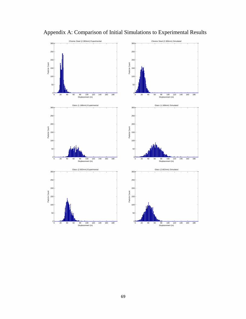
69

Appendix A: Comparison of Initial Simulations to Experimental Results

0 20 40 60 80 100 120 140 160 1800

50

100

150

200

250

300

Displacement (in)

Part

icle

Count

Chrome Steel (2.383mm) Experimental

0 20 40 60 80 100 120 140 160 1800

50

100

150

200

250

300

Displacement (in)

Part

icle

Count

Chrome Steel (2.383mm) Simulated

0 20 40 60 80 100 120 140 160 1800

50

100

150

200

250

300

Displacement (in)

Part

icle

Count

Glass (1.168mm) Experimental

0 20 40 60 80 100 120 140 160 1800

50

100

150

200

250

300

Displacement (in)

Part

icle

Count

Glass (1.168mm) Simulated

0 20 40 60 80 100 120 140 160 1800

50

100

150

200

250

300

Displacement (in)

Part

icle

Count

Glass (2.602mm) Experimental

0 20 40 60 80 100 120 140 160 1800

50

100

150

200

250

300

Displacement (in)

Part

icle

Count

Glass (2.602mm) Simulated

70

0 20 40 60 80 100 120 140 160 1800

50

100

150

200

250

300

Displacement (in)

Part

icle

Count

Glass (3.646mm) Experimental

0 20 40 60 80 100 120 140 160 1800

50

100

150

200

250

300

Displacement (in)

Part

icle

Count

Glass (3.646mm) Simulated

0 20 40 60 80 100 120 140 160 1800

50

100

150

200

250

300

Displacement (in)

Part

icle

Count

Glass (5.995mm) Experimental

0 20 40 60 80 100 120 140 160 1800

50

100

150

200

250

300

Displacement (in)

Part

icle

Count

Glass (5.995mm) Simulated

0 20 40 60 80 100 120 140 160 1800

50

100

150

200

250

300

Displacement (in)

Part

icle

Count

Zirconia-Silica (1.121mm) Experimental

0 20 40 60 80 100 120 140 160 1800

50

100

150

200

250

300

Displacement (in)

Part

icle

Count

Zirconia-Silica (1.121mm) Simulated

0 20 40 60 80 100 120 140 160 1800

50

100

150

200

250

300

Displacement (in)

Part

icle

Count

Zirconia (1.072mm) Experimental

0 20 40 60 80 100 120 140 160 1800

50

100

150

200

250

300

Displacement (in)

Part

icle

Count

Zirconia (1.072mm) Simulated