modeling the spatial dependency of shopping center trade areas
TRANSCRIPT

Modeling the Spatial Dependency of Shopping Center Trade Areas
Burcu H. OZUDURU
Gazi University Faculty of Engineering and Architecture Department of City and Regional Planning
Maltepe/ANKARA/TURKEY E-mail: [email protected]
Jean-Michel GULDMANN
The Ohio State University Knowlton School of Architecture
Department of City and Regional Planning, Columbus/OHIO/USA
E-mail: [email protected]
The shopping habits of consumers residing in one geographical area, and shopping in another appears as a major problem in retail activity modeling, and is referred to as spatial dependency of shopping center trade areas. The level of dependency is crucial in delineation of the trade area boundaries for retailers to obtain realistic information on the spatial behavior of consumers, and a better direction for formulation of the retail development strategy. As a rule of thumb, the dependency increases when the spatial scale is smaller and the geographical units are distant from each other, such as in rural areas. The literature presents such studies at state, statistical metropolitan area and rural county levels. However, it does not present any models to assess the level of dependency at smaller units. This study aims to uncover various levels of spatial dependency across shopping center trade areas in Ohio: at county(CTY) and zipcode(ZCU) levels. At the CTY level, recursive equation models and at the ZCU level, simultaneous equation models and spatial regression models with retail gravity indices are used. The results show that the level of dependency is identified more clearly at the ZCU level than at the CTY level, pointing to a competitive substitution between retail systems across ZCUs. Additionally, the models show that a new retail gravity index is useful to assess the level of dependency at the ZCU level. These results can be used by decision makers for commercial zoning policy, shopping center site selection, and can be incorporated into urban policy making processes.
Keywords: retail activity, spatial dependence, retail gravity index.

2
1- INTRODUCTION Location decisions play a vital role in success and failure of shopping centers and
require a complex evaluation process. An effective strategy involves many variables, because costs are quite high and there is less flexibility once sites are chosen. To develop an effective retail strategy, decision makers must select attractive store locations and utilize marketing mix factors in the most effective way. They need to identify these location characteristics and understand the dynamics of the retail structure, in particular, the basic premises for the success of shopping centers and how shopping centers interact with other urban systems. An analysis of smaller geographical units and a more site-specific research reveal more information on the TAs of the shopping centers. Various TA models can be formulated with this purpose.
In this paper, Oppenheim’s (1991) retail activity allocation model is used as a conceptual framework to empirically measure the level of spatial interdependency across counties (CTYs) and zip codes (ZCUs) in Ohio. Oppenheim formulates his model by analyzing the relationships between supply and demand factors of a hypothetical commercial activity and travel system. With his model, he assesses the impact of various changes in physical and economic conditions in this hypothetical system.
The spatial interdependencies among retailers and consumers of a given area and its surrounding areas in CTYs and ZCUs are incorporated into the model by using simultaneous equations. At the county level, the surrounding area represents all the neighboring counties; at the zip code level, it refers to all of the surrounding areas within 5-, 10-, and 15- miles of the given zip code boundary.
At the zip code level, a new gravity index measuring the level of spatial interdependency across ZCUs is introduced. This index measures the market potential of the surrounding ZCUs within 20- and 30- miles of the given ZCU centroid, using retail sales, household disposable income and distance. The model is formulated by including trade area demand characteristics and this index into multiple regression analyses.
The use of TA models in retail market analysis has received a lot of attention from market researchers, business analysts, developers, investors and retailers, who have tried to answer the question, whether the center will succeed by capturing the necessary amount of market share and analyzed the factors effective in increasing the market share (Schmitz and Brett 2002). However, the spatial dependency among trade areas, in other words, the relationship between shopping centers in a place and its adjacent market areas, has always been an issue and many researchers have tried to overcome this problem.
The phenomenon is also referred to as consumer out-shopping (Russell 1957; Anderson and Kaminsky 1985; Ghosh and McLafferty 1987; Mejia and Benjamin, 2002), addressing the fact that some consumers buy goods and services away from their homes that could be purchased locally, retail leakage among communities (Ingene and Lusch, 1980; Lillis and Hawkins 1974), or geographical interdependency (Mushinski and Weiler 2002).
Previous research has gone in two ways. The first group explains who the out-shoppers are, and why they shop outside, thus investigating the demographic, socio-economic and psychographic aspects of the phenomenon (Herrmann and Beik 1968; Thompson 1971; Samli and Uhr 1974; Lau and Yau 1985). The second group, however, adopting a broader perspective and accounting for economic relations, examines the retail market conditions and influence of out-shopping on local markets (Papadopoulos 1980;
3
Jarratt 1998, 2000). Only a few empirical models assess the geographical interdependency of retailers across selected areas (Anderson and Kaminsky 1985; Mushinski and Weiler 2002; Adamchak et al. 1999). In particular, Mushinski and Weiler (2002) define a model measuring the level of geographical interdependency both on supply and demand side across specific retailing business establishments. Accounting for this interdependency provides a better estimate of the retail sales and helps to identify the relationship between TA characteristics and shopping center attributes. In Ferber’s (1958) study, it distorts the research results.
The literature does not present new methods to assess the level of spatial or geographical interdependency. More specifically, there are not any empirical studies and models for geographical dependency assessment across smaller units, which point to higher interdependency and more ambiguous trade area relationships. However, such studies will provide a better direction for formulating the retail strategy in a market, thus will be useful to the actors involved in the decision process.
This paper, in contrast to previous research, including all of the shopping centers, and using both metropolitan and non-metropolitan geographical units, adopts two different methods to measure the geographic interdependency and finds significant results. The major advantage of ZCUs is that, in contrast to cities/places, they make up a continuous geographical coverage, thus can be easily aggregated into trade areas, and are more site-specific and useful for analysts, developers, investors, and retailers.
In this paper, first, the existing literature on out-shopping and geographical interdependency across trade areas is reviewed. Next, the methodology and database are described, followed by the model specifications and empirical findings. The paper concludes with a discussion of theoretical and managerial implications.
2- LITERATURE REVIEW Earlier retailing studies focus on the impact of: (1) city size and (2) distance on
the shopping center preferences of shoppers (Reilly 1931; Huff 1963, 1964). However, individual shopper responses to the drawing power of urban centers and type of goods are equally important to explain these preferences (Herrmann and Beik 1968) and should be accounted for in TA analyses. Consumers buy goods and services outside their local community. For the first time in the literature, Russell (1957) relates consumer out-shopping to geographical interdependency of trade areas in urbanized areas for retail establishments. Her findings reveal that measuring the level of geographical interdependency generates more reliable profile of the customers and the boundaries of the TA, which is important for site selection and retail strategy making.
Harris and Shonkwiler (1997) suggest that the interdependency among a community’s businesses and between businesses and service facilities is important for the local retail sector viability and vitality, and develop analytical procedures that would incorporate retail business interdependencies in TA analysis. Lee and Pace (2005) investigate spatial dependency among consumers and stores by developing four gravity models, and show that the spatial dependency hypothesis results in far more plausible parameter estimates than assuming independency.
Several researchers have analyzed reasons of the characteristics of the consumers and found that out-shopping originates either from demographic characteristics of consumers, such as income, age, education or from their specific attitudes towards

4
marketing principles of local retailers, such as dissatisfaction with the selection, price, service, and quality of the local shopping alternatives (Lillis and Hawkins 1974; Jarratt 1996; Thompson 1971; and Herrmann and Beik 1968).
As a rule of thumb, geographical dependency increases when the spatial scale is smaller (i.e. cities have higher dependency than counties or metropolitan areas; zip codes have higher dependency than cities). A small market size points to smaller assortment of goods and services (Papadopoulos 1980), such as in rural areas, fewer retailers supply goods and services (Polonsky and Jarratt 1992). Out-shopping appears as a problem specifically for small business retailers (Anderson and Kaminsky 1985). In their analysis of department store markets, Ingene and Lusch (1980) use MSAs as the geographical unit, pointing out that cities and counties are too small, because considerable shopping occurs across their boundaries and there is more ‘leakage’.
Anderson and Kaminsky (1985) use county-level data, Mushinski and Weiler (2002) and Harris and Shonkwiler (1997) include geographically isolated communities distinct from metropolitan statistical areas (MSAs) to allow a clearer focus on consumer demand and retail supply interactions between distinct places and their hinterlands.
Geographical interdependency has been measured by using (1) models, and (2) indices. Mushinski and Weiler (2002) describe geographical interdependency of retail market areas and sectors in a CTY by dividing the CTY into two parts: (1) place and (2) neighboring areas. They use a “Simultaneous Equation Tobit Model” and find that geographical interdependency between a place and its neighboring areas varies across retail sector groups and that both the number of establishments and the population in neighboring areas has a significant impact on the number of establishments in the place.
Polonsky and Jarratt (1992) and Anderson and Kaminsky (1985) use various indices to estimate the level of out-shopping in rural areas. Polonsky and Jarratt analyze rural out-shopping in a particular region in Australia, by calculating the Net Trade Flow (NTF), which is the net effect of in-shopping of an area’s inhabitants. They also use Sales Conversion Index (SCI) to allow for comparison across cities, regions. Anderson and Kaminsky (1985), in a descriptive framework, examine the characteristics of out-shoppers, analyze the type of goods and services that they prefer, and specify the retailers that attract them by the ratio of out-shoppers to in-shoppers, and buying power index1. Herrmann and Beik (1968) utilize the ratio of purchases and shoppers out of town. Jarratt (2000) identifies direct and indirect relations between shopping areas and shopper preferences. Jarratt (2000), in a consumer behavior-oriented research, constructs Comparative Fit Indices (CFIs – goodness of fit measures) to find out which shopping variables have an impact on the level of out-shopping. Then, a structural equation model (SEM) is defined with the more prominent variables. The use of such variables indicates that the measurement of geographical interdependence is useful in identifying the market relations in a selected TA.
Literature does not present any ZCU level analysis; however, this paper will present a different approach where the dependency across both metropolitan and non-metropolitan CTYs and ZCUs are assessed. Additionally, both modeling techniques and
1 Buying Power is the ratio of retail sales to effective buying income (Anderson and Kaminsky, 1985, p. 39).

5
indices are going to be used to assess the relationship between the trade area characteristics of these CTYs and ZCUs. In the following section, the methodology is explained.
3- METHODOLOGY The primary goal of this study is to determine the level of geographical
interdependency across CTYs and ZCUs. In this section, first the retail activity allocation model of Oppenheim (1991) is briefly explained. Then, general specifications of simultaneous equation models described. Finally, the computation of the retail gravity index is presented. 3.1. Retail Activity Allocation Model
In line with the basic equilibrium principle of Oppenheim (1991), for each shopping center, the total revenues from retail expenditures by the population,
!
Yij , must be equal to the cost of retail supply, which is assumed to be a direct function of the size of the shopping center. This cost is taken as a power function of
!
X j , and the basic equilibrium equations are:
!
Ri
i=1
n
" eiX j
#exp($Cij )
X j
#exp($Cij )
j
"
%
&
' ' '
(
)
* * *
= bX j
q
!
j =1" m (1)
where
!
X j is the size of the shopping facility in zone
!
j ,
!
Cij is the travel time or cost between i and j,
!
" and
!
" are the parameters,
!
Ri is the residential population in zone
!
i , and
!
ei is the retail spending per capita in zone
!
i , b is a parameter with the dimension of a unit cost, q is a parameter measuring economies and diseconomies of scale in the operation of the shopping center. There are
!
m equations (3), with
!
m unknowns (
!
X j ), hence, in principle, a unique solution.
A generalized retail supply function is formulated, where the focus is on the variables
!
X = X j j =1" m{ }. For any given set of values for the exogenous parameters
would produce a specific solution X*
!
= X j{ } , and varying these input parameters would lead to different solutions. Therefore, each solution variable
!
X j
* is implicitly a function of the input parameters, with:
!
X j
* = Fj (R, e, σ, β, α , Z, q, C(0), Y(0), c, a, b) (2)
The exogenous parameters can be subsumed into three vectors: Population: P = {R, e, σ , β , α}
Shopping Center: R = {Z, b, q} Transportation: T = {C(0), Y(0), c, a, b}
6
Vector P characterizes the geographical distribution of the population throughout the urban/metro area, and the behavioral characteristics of its various socio-economic groups. Vector R characterizes the various (given) shopping center sites. Vector T characterizes the whole urban/metro transportation system. Equation (2) can be reformulated as:
!
X j
*= Fj(P, R, T) (3)
The conceptual framework illustrated by Equation (3) provides the basis for developing retail supply functions that can be estimated empirically.
3.2. Generalized Specifications
In a self-contained geographical urban area,
!
u , the exogenous parameters are indexed by
!
u . Equation (3) can be reformulated as:
!
X ju
*= Fj(Pu, Ru, Tu) (4)
The total retail supply for urban area
!
u is then:
!
XTOT ,u
*= X ju
*
j=1
m
" = Fj
j=1
m
" ( Pu, Ru, Tu) = F(Pu, Ru, Tu) (5)
When data are available on
!
XTOT
* and (P, R, T) for a sample of such self-contained urban areas
!
(u =1"U) , it is possible to test and estimate various specifications of the function F (e.g., linear, log-log, etc.). Such empirically estimated functions would point to the impact of various urban-wide variables on the equilibrium supply of retail space accommodations.
3.3. Trade Area Interdependency
3.3.1. Simultaneous Equations. When the self-contained urban area
!
u is subdivided into a few major sub areas
!
(s =1" S), Equation (4) can be aggregated over each of the s sub areas, with:
!
Xsu
*= X ju
*
j"S
# =Gs(Pu, Ru, Tu)
!
(s =1" S), (6)
Equation (5) represents a system of
!
S individual equations. This system can be viewed as the reduced form of a system of simultaneous equations, where the retail supply in sub area
!
s is a function of (1) the retail supply in all other areas, and (2) the exogenous variables (Pu, Ru, Tu), disaggregated by sub area. This approach is consistent with the approach used by Mushinski and Weiler (2002), although their argument does not rely on a formal derivation from a mathematical model, but rather on general central place theory ideas. Let X*
NS,u be the vector of the retail supplies in all sub areas, except
!
s. Equation (6) is then reformulated as:
!
Xsu
*=G(X*
NS,u, Pus, Rus, Tus
!
s =1" s) (7)
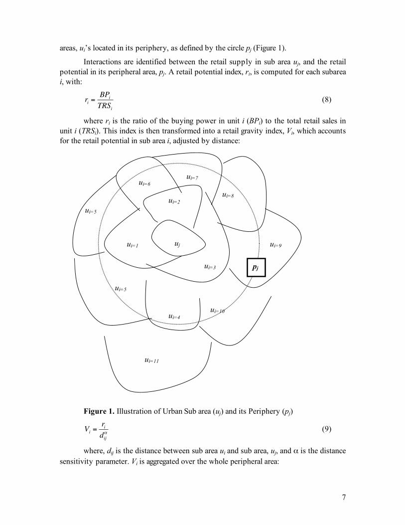
3.3.2. Gravity Index. In this model, the geographic interactions across boundaries are treated differently. Assume that the urban subarea uj is dependent on other urban sub
7
areas, ui’s located in its periphery, as defined by the circle pj (Figure 1).
Interactions are identified between the retail supply in sub area uj, and the retail potential in its peripheral area, pj. A retail potential index, ri, is computed for each subarea i, with:
!
ri=BP
i
TRSi
(8)
where ri is the ratio of the buying power in unit i (BPi) to the total retail sales in unit i (TRSi). This index is then transformed into a retail gravity index, Vi, which accounts for the retail potential in sub area i, adjusted by distance:
Figure 1. Illustration of Urban Sub area (uj) and its Periphery (pj)
!
Vi =ri
dij"
(9)
where, dij is the distance between sub area ui and sub area, uj, and α is the distance sensitivity parameter. Vi is aggregated over the whole peripheral area:
uj
ui=1
ui=2
ui=3
ui=4
ui=5
ui=5
ui=6
ui=7
ui=8
ui=9
ui=10
ui=11
pj

8
!
VSp = Vi" (10)
where, VSp is the total retail potential index of the peripheral area. This index is incorporated into the model as a separate variable, along with the exogenous variables characterizing sub area uj. Equation (4) is reformulated as:
!
Xuj
*= Fj (P
!
u j , R
!
u j , T
!
u j , VSp) (11)
Equation (11) represents a model where the retail supply in a sub area is dependent on both these sub area variables and the peripheral area retail potential, and where the level geographical dependency between the sub area and its peripheral area is identified through the retail gravity index.
4- DATA Four primary databases, all pertaining to the year 2000 are used in this study. The
geographic focus is the state of Ohio. 1) Directory of Major Malls (DMM); 2) National Research Bureau (NRB); 3) United States Census of Population and Housing; and 4) Demographics U.S.A. The DMM and NRB databases are combined in a final database of all shopping centers, providing information on physical and geographic attributes of all shopping centers in Ohio. The socioeconomic, demographic and housing-related characteristics are extracted from the U.S. Census 2000. Finally, the Demographics U.S.A. database is used as a collection of marketing statistics directories, providing data on some retail trade variables, such as total retail sales, total effective buying income, median household effective buying income, population by effective buying income groups, and total expenditures.
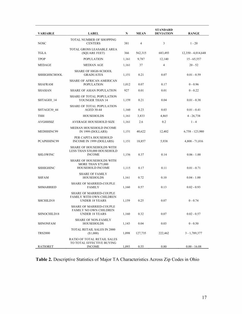
The final database contains 1,391 shopping centers. The state of Ohio is composed of 88 counties, and 81 (92%) of these counties include at least one shopping center. 88.4% of the centers are in metropolitan counties and 11.6% are in non-metropolitan counties. Additionally, the state of Ohio is composed of 1,189 ZCUs, and nearly one third (381) of these units contain one or more shopping centers.
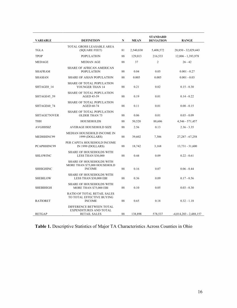
<<Table 1. Descriptive Statistics of Major TA Characteristics Across CTYs in Ohio>>
<<Table 2. Descriptive Statistics of Major TA Characteristics Across ZCUs in Ohio>>
5. EMPIRICAL MODEL SPECIFICATIONS 5.1. Multiple Regression Model
Based on the equilibrium principle of the conceptual model, for each area (CTY or ZCU) the total retail supply is related to the total demand characteristics. The generalized retail supply function derived in Section 3.1 is specified as a multiple regression model to conduct the empirical analyses. The independent variables are restricted to the population vector P.
The empirical analyses include n (i=1→n) ZCUs. Each ZCU, i, has m (j=1→m) shopping centers. The total size of the shopping center system in area i, is measured by
9
the total gross leasable area,
!
TGLAi = GLA j
j=1
m
" . The socio-economic characteristics of the
TA, such as population, income, household size, median age, etc. make up the vector P = {P1, … Pn}. Equation (5) is transformed into a double-log model, with:
lnTGLA = α0 + α1 ln P1 + α2 ln P2 +….+ αn ln Pn (12)
5.2. Geographical Interdependency 5.2.1. Simultaneous Equations. The existence of the certain level of geographic interdependency across retail markets located in neighboring CTYs and ZCUs is tested by using a simultaneous equation modeling approach. The CTYs and ZCUs in neighboring states are not included in the analyses, thus ignoring possible geographic interdependencies between states. The TGLA in each CTY/ZCU, and the TGLA in the surrounding CTY/ZCUs, STGLA, are the endogenous variables in the simultaneous equations. STGLA characterizes the TGLA in all the adjacent CTYs/ZCUs.
Together with these endogenous variables, a number of exogenous (predetermined) variables are verified. These variables pertain to two groups: (1) Population: This variable is the most important determinant of TGLA in CTYs/ZCUs. Two variables are introduced: (i) the population in the CTY/ZCU, (ii) the population in the surrounding CTY/ZCU. (2) Retail Sales Potential: These variables include the discretionary income ratio, and the median effective buying income in the CTY/ZCU.
The simultaneous equations at the CTY/ZCU levels are formulated as follows: TGLAi = F (STGLAi, Pi, SPi) (13)
STGLAi = F (TGLAi, SPi, Pi) (14) TGLAi is the total gross leasable area in CTY/ZCU i, STGLAi is the total gross
leasable area in the surrounding CTYs/ZCUs, Pi is the vector of demographic and socioeconomic characteristics in i, and SPi is the vector of demographic and socioeconomic characteristics in the CTYs/ZCUs surrounding CTY/ZCU i. Pi is composed of population and retail sales potential variable for CTY/ZCU i, and SPi includes the total population of the surrounding CTYs/ZCUs.
There are two statistical issues related with the model: (1) The standard regression models, estimated by the ordinary least squares (OLS) method, are corrected for heteroscedasticity2. (2) The structural models represented by Equations (13) - (14) can be transformed into reduced-form equations3.
2 OLS method assumes that the error terms are normally distributed, with a zero expected value and a constant variance. The assumption of constant error variance, or homoscedasticity, may not hold for cross-sectional data when the scale of a variable varies substantially within the sample. This might be the case of county populations, with larger populations involving more volatility, hence larger error variances. The logarithmic transformation reduces the variation in the variables, hence may remove heteroscedasticity. If
10
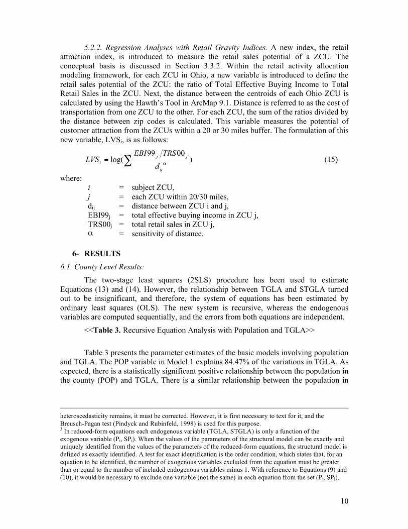
5.2.2. Regression Analyses with Retail Gravity Indices. A new index, the retail attraction index, is introduced to measure the retail sales potential of a ZCU. The conceptual basis is discussed in Section 3.3.2. Within the retail activity allocation modeling framework, for each ZCU in Ohio, a new variable is introduced to define the retail sales potential of the ZCU: the ratio of Total Effective Buying Income to Total Retail Sales in the ZCU. Next, the distance between the centroids of each Ohio ZCU is calculated by using the Hawth’s Tool in ArcMap 9.1. Distance is referred to as the cost of transportation from one ZCU to the other. For each ZCU, the sum of the ratios divided by the distance between zip codes is calculated. This variable measures the potential of customer attraction from the ZCUs within a 20 or 30 miles buffer. The formulation of this new variable, LVSi, is as follows:
!= )0099
log("
ij
jj
id
TRSEBILVS (15)
where: i = subject ZCU, j = each ZCU within 20/30 miles, dij = distance between ZCU i and j, EBI99j = total effective buying income in ZCU j, TRS00j = total retail sales in ZCU j, α = sensitivity of distance.
6- RESULTS
6.1. County Level Results: The two-stage least squares (2SLS) procedure has been used to estimate
Equations (13) and (14). However, the relationship between TGLA and STGLA turned out to be insignificant, and therefore, the system of equations has been estimated by ordinary least squares (OLS). The new system is recursive, whereas the endogenous variables are computed sequentially, and the errors from both equations are independent.
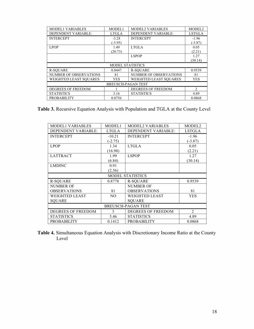
<<Table 3. Recursive Equation Analysis with Population and TGLA>>
Table 3 presents the parameter estimates of the basic models involving population and TGLA. The POP variable in Model 1 explains 84.47% of the variations in TGLA. As expected, there is a statistically significant positive relationship between the population in the county (POP) and TGLA. There is a similar relationship between the population in
heteroscedasticity remains, it must be corrected. However, it is first necessary to text for it, and the Breusch-Pagan test (Pindyck and Rubinfeld, 1998) is used for this purpose. 3 In reduced-form equations each endogenous variable (TGLA, STGLA) is only a function of the exogenous variable (Pi, SPi). When the values of the parameters of the structural model can be exactly and uniquely identified from the values of the parameters of the reduced-form equations, the structural model is defined as exactly identified. A test for exact identification is the order condition, which states that, for an equation to be identified, the number of exogenous variables excluded from the equation must be greater than or equal to the number of included endogenous variables minus 1. With reference to Equations (9) and (10), it would be necessary to exclude one variable (not the same) in each equation from the set (Pi, SPi).
11
the surrounding counties (SPOP) and STGLA. In addition, TGLA is positively related to STGLA.
The reduced forms of Models 1 and 2 are: TGLA = -3.28 + 1.49(POP) (16)
STGLA = -2.12 + 0.07(POP) + 1.27(SPOP) (17) Equations (16) and (17) indicate that TGLA is positively related to POP and
STGLA is positively related to both POP and SPOP. An increase in the central county population (POP) leads to a very small increase in the surrounding counties retail supply (STGLA), pointing to a small complementary effect.
<<Table 4. Simultaneous Equation Analysis with Discretionary Income Ratio>> When the discretionary income ratio (ATTRACT), defined as the ratio of total
retail sales to total effective buying income, and the median household effective buying income (MDINC) are included in the analysis, POP remains significant in Model 1 (Table 4). The ratio, which has a positive and significant effect on TGLA, measures the market potential of the central county. MDINC, which also has a positive and significant effect on TGLA, is an indicator of the available income for retail purchases in the central county. These two variables are not included in Model 2 because they measure the central county characteristics. Model 2 includes both SPOP and STGLA as independent variables. The reduced forms of the models are:
TGLA = -10.21 + 1.34(POP) + 1.99(ATTRACT) + 0.91(MDINC) (18) STGLA = -2.47 + 0.07(POP) + 0.10(ATTRACT) + 0.05(MDINC) + 1.27(SPOP) (19)
The reduced form in Equation (19) indicates that POP, ATTRACT and MDINC have positive but weak effects on STGLA, in contrast to strong effects on TGLA in Equation 18. The relationship between STGLA and SPOP is very similar to POP and TGLA.
6.2. Zip Code Level Results: 6.2.1. Simultaneous Equations. The simultaneous equations (13) and (14) are specified as follows. The exogenous variables in Equation (13) include (1) the population (POP), (2) the discretionary income ratio (ATTRACT), (3) the median effective buying income, and (4) the area (AREA) of the central ZCU. The ATTRACT and MDINC variables represent market potential indicators of the central ZCU, and the AREA variable accounts for the ZCU population density. ATTRACT is the ratio of total retail sales to total effective buying income. The system of equations is estimated with 2SLS for each buffer case. The results are presented in Table 7.
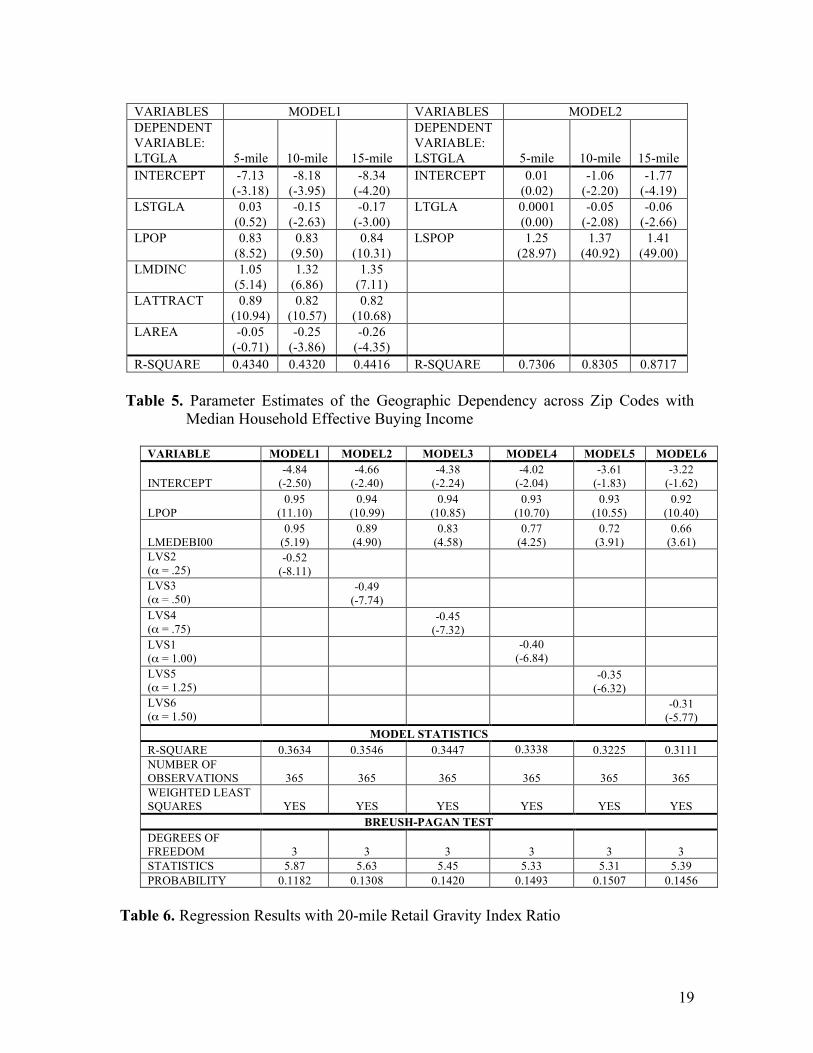
<< Table 5. Parameter Estimates of the Geographic Dependency across Zip Codes with
Median Household Effective Buying Income >> STGLA has a statistically significant and negative relationship with TGLA in the
10- and 15-mile buffer cases. However, its elasticity is small. A 1% increase in STGLA

12
within 10- or 15-mile buffers of the ZCU leads to a 0.15% to 0.17% decrease in TGLA, pointing to the importance of competition across ZCUs within 10 and 15 miles.
In contrast to the previous analysis, the R2 is the lowest in the 10-mile buffer case and the highest in the 15-mile case in Model 1. The elasticity of ATTRACT is positive and significant in all cases, varying between 0.82 and 0.89, and highest in the 5-mile buffer case. This result can be explained by the primary TA boundaries of shopping centers. It has been observed that the primary TA corresponds to a radius of 5 miles. While people travel to other ZCUs for shopping, the sales within the immediate area of the shopping center are still the most crucial factor in shopping center developments.
The MDINC variable is positively related to TGLA in all cases. Its elasticity varies from 1.05 to 1.35. The R2 of Model 1 varies between 0.432 and 0.442, the 15-mile R2 is the highest and points out that the area within the 15-mile is also important for shopping center developments.
The area of the central ZCU (AREA) is significant in both the 10- and 15-mile buffer cases, but insignificant in the 5-mile case. It has a negative relationship with TGLA. A 1% increase in AREA leads to a 0.25-0.26% decrease in TGLA. This relation points to the negative relationship between the population density and available retail space. If the density of a ZCU is low, it is less likely to attract developers, because it is more costly for customers to commute to the shopping center and the retailers/developers prefer to have the highest proximity to the highest number of customers, to attain the highest possible profits.
In Model 2, the strong relationship between SPOP and STGLA and the negative relationship between TGLA and STGLA remain, pointing to a competitive effect among retail systems. The significance levels of the variables increase by distance. The 15-mile buffer case generates the highest parameter coefficients. The reduced forms for the 15-mile buffer case are:
TGLA= -8.12 + 0.85(POP) + 1.37(MDINC) + 0.83(ATTRACT) – 0.26(AREA) - 0.24(SPOP) (20) STGLA= -1.31 – 0.05(POP) - 0.08(MDINC) – 0.05(ATTRACT)
+ 0.01(AREA) + 1.42(SPOP) (21)
The reduced equations indicate that TGLA is positively related to POP and the retail potential characteristics of the ZCU, MDINC and ATTRACT, and negatively related to AREA and SPOP. The effect of MDINC and ATTRACT on TGLA is much stronger in Equation 20 than in Equation 21, where they have a negative and weak effect on STGLA. The elasticity of SPOP is much stronger in Equation 21 and is positive, as expected. 6.2.2. Regression Analyses with Retail Gravity Variables Results. As outlined in Equations 8 through 11, a new gravity-based variable is included in the regression analyses, together with two basic variables, population and income. The analyses are conducted for 20-miles and 30-miles buffers. In order to test the effect of distance, which

13
is used to derive the new variables, several exponent α values are considered alternatively.
Retail Gravity Index with a 20-mile Buffer. Initially, the models are estimated with twelve values of α (0.25, 0.50, 0.75, 1.00, 1.25, 1.50). As expected, the population and median EBI variables have statistically significant and positive relationships with TGLA. The LVS variable, which measures the level of geographic dependency between the central ZCU and its surrounding ZCUs within the 20-mile buffer, has a statistically significant and negative relationship with TGLA. LVS is a measure of the discretionary income available within the 20-miles buffer. Its increase is likely to lead to new shopping center development within the buffer, which will reduce the number of shoppers from the buffer to the central ZCU. The best model (R2=0.363) is obtained with α = 0.25 (Table 6).
<< Table 6. Regression Results with 20-mile Retail Gravity Index Ratio >>
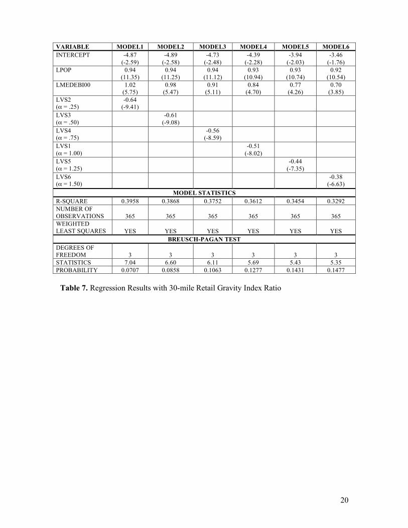
Retail Gravity Index with a 30-mile Buffer. The parameter estimates and the R2 are substantially higher for the 30-mile buffer, as compared with the 20-mile buffer. The results are presented in Table 7. Again the highest R2 (0.396) is obtained when α = 0.25. This result points out the importance of properly identifying trade areas to measure trade interaction.
<< Table 7. Regression Results with 30-mile Retail Gravity Index Ratio >>
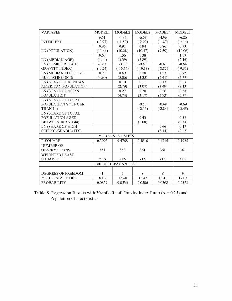
6.2.3. Retail Ratio Gravity Index (α = 0.25) with a 30-mile Buffer and Population Characteristics. The inclusion of Census variables with the best 30-mile Retail Gravity Index, where α = 0.25, increases the R2 of the models substantially. The results are presented in Table 7. Models 1 through 5 have R2 varying from 0.39 to 0.49. The variables have the expected elasticities and significances, except for the share of total population aged between 30 and 44. Model 4 generates the highest R2 with the highest number of significant variables, thus is the best model. The median age and the share of total population aged between 30 and 40 are dropped in this model and the R2 is 0.47, approximately 10% more than Model 1 in Tables 6 and 7. The number of households and household characteristics were considered as well, but did not generate as high explanatory powers as population and population characteristics.
<< Table 8. Regression Results with 30-mile Retail Gravity Index Ratio (α = 0.25) and
Population Characteristics >>
7- CONCLUSION In retail strategy making, understanding TA relations and selecting the best
location are important. This has an impact on urban policy-making and urban development. If customers in a TA prefer to shop at a different TA, pointing to the fact that existing retail outlets are not fulfilling the customer needs, the decision makers should improve their management strategies and location preferences.
14
This paper presents a modeling technique for assessing the level of spatial interdependency of customers at various geographical levels. The models are formulated at county (CTY) and zip code (ZCU) levels, assuming that a trade area is a combination of these units, and the database for the empirical analyses includes a combination of retail marketing variables, such as population, income, total expenditures in the CTY/ZCU, etc. in Ohio, USA.
The results show that the spatial interdependency across CTYs is less than that of ZCUs, as expected. The positive parameter estimates of TGLA in recursive equations in Model 2 (Table 3 and 4), a 1% increase in TGLA, increases the STGLA by 0.05%, points out that out-shopping across counties is not an issue, and that there is a small complementary effect across counties. However, at the ZCU level, the TGLA at the ZCU and the TGLA at the surrounding 15-mile has a strong negative relation, pointing to the fact that a shopping center can attract consumers from the 15-mile extension of the ZCU boundary. Therefore, any shopping center built within 15-miles of the ZCU can be the competitor of the shopping center at the central ZCU. For example, a 1% increase in the surrounding retail space corresponds to a 0.17% decrease in the ZCU retail space (Table 5). The same competitive substitution between retail systems across ZCUs also appears in 10-mile results.
The second model results show that a new retail potential index is useful to identify the level of the spatial interdependency. The inclusion of such variable increases the explanatory power of the models at the ZCU level. The highest explanatory power is achieved when the distant exponent α is 0.25. The explanatory power of this model increases with the inclusion of population characteristics variables. The R2 increases substantially from 0.39 to 0.49. The explanatory power of household characteristics is smaller than that of population characteristics, pointing to the fact that population characteristics are better explanatory variables.
The R2 also explains the level of spatial interdependency. At the CTY level, the it varies from 0.84 to 0.95, as compared to 0.43 to 0.87 at the ZCU level. This shows that the interdependency across the retail markets located in neighboring areas increases as the unit size gets smaller.
In contrast to earlier studies, this research provides a novel approach to measure the relationships between TA characteristics and shopping center attributes. First, these relationships focus on smaller geographic units, counties and zip codes. In past studies, smaller geographical units have been avoided due to higher levels of interdependency across these units, as compared to MSA or state levels. ZCU analyses of shopping centers and TAs have been avoided due to high geographical interdependency levels. In addition, in this study, both metropolitan and non-metropolitan shopping center systems are considered, whereas the literature points to non-metropolitan areas in most cases. Finally, all types of shopping centers are included in the empirical model instead of a particular chain/store or center type.
The results of this research may be helpful to retailers/developers and decision makers and be used as a tool to assess the impact of changes in TA characteristics on shopping center attributes, including the population and population characteristics, household and household type characteristics, and income variables. Model results can help assess the excess or deficiency of a given area in commercial floor space, and thus

15
serve as a basis for decisions by developers, and as a basis for commercial zoning by public officials. Additionally, given the demand characteristics in a CTY/ZCU in Ohio, the developers can assess the amount of the retail investment necessary for the area. Public officials can test the development proposals in response to the results of this research models. Therefore, these models can be used in urban policy making and retail strategy formulation.
16
VARIABLE DEFINITION N MEAN STANDARD DEVIATION RANGE
TGLA TOTAL GROSS LEASABLE AREA
(SQUARE FEET) 81 2,540,830 5,408,572 28,850 - 32,029,443
TPOP POPULATION 88 129,013 216,533 12,806 - 1,393,978
MEDAGE MEDIAN AGE 88 37 2 26 - 42
SHAFRAM SHARE OF AFRICAN AMERICAN
POPULATION 88 0.04 0.05 0.001 - 0.27
SHASIAN SHARE OF ASIAN POPULATION 88 0.005 0.005 0.001 - 0.03
SHTAGE0_14 SHARE OF TOTAL POPULATION
YOUNGER THAN 14 88 0.21 0.02 0.15 - 0.30
SHTAGE45_59 SHARE OF TOTAL POPULATION
AGED 45-59 88 0.19 0.01 0.14 - 0.22
SHTAGE60_74 SHARE OF TOTAL POPULATION
AGED 60-74 88 0.11 0.01 0.08 - 0.15
SHTAGE75OVER SHARE OF TOTAL POPULATION
OLDER THAN 75 88 0.06 0.01 0.03 - 0.09
THH HOUSEHOLDS 88 50,520 88,606 4,546 - 571,457
AVGHHSIZ AVERAGE HOUSEHOLD SIZE 88 2.56 0.13 2.36 - 3.35
MEDHHINC99 MEDIAN HOUSEHOLD INCOME IN
1999 (DOLLARS) 88 39,602 7,306 27,287 - 67,258
PCAPHHINC99 PER CAPITA HOUSEHOLD INCOME
IN 1999 (DOLLARS) 88 18,742 3,168 13,731 - 31,600
SHLOWINC SHARE OF HOUSEHOLDS WITH
LESS THAN $30,000 88 0.44 0.09 0.22 - 0.61
SHHIGHINC
SHARE OF HOUSEHOLDS WITH MORE THAN $75,000 HOUSEHOLD
INCOME 88 0.16 0.07 0.06 - 0.44
SHEBILOW SHARE OF HOUSEHOLDS WITH
LESS THAN $30,000 EBI 88 0.36 0.09 0.17 - 0.56
SHEBIHIGH SHARE OF HOUSEHOLDS WITH
MORE THAN $75,000 EBI 88 0.10 0.05 0.03 - 0.30
RATIORET
RATIO OF TOTAL RETAIL SALES TO TOTAL EFFECTIVE BUYING
INCOME 88 0.65 0.18 0.32 - 1.18
RETGAP
DIFFERENCE BETWEEN TOTAL EXPENDITURES AND TOTAL
RETAIL SALES 88 138,898 578,537 -4,014,203 - 2,488,157
Table 1. Descriptive Statistics of Major TA Characteristics Across Counties in Ohio
17
VARIABLE LABEL N MEAN STANDARD DEVIATION RANGE
NOSC TOTAL NUMBER OF SHOPPING
CENTERS 381 4 3 1 - 20
TGLA TOTAL GROSS LEASABLE AREA
(SQUARE FEET) 366 562,315 683,493 12,350 - 4,014,648
TPOP POPULATION 1,161 9,787 12,140 15 - 65,557
MEDAGE MEDIAN AGE 1,161 37 4 20 - 52
SHHIGHSCHOOL SHARE OF HIGH-SCHOOL
GRADUATES 1,151 0.21 0.07 0.01 - 0.59
SHAFRAM SHARE OF AFRICAN AMERICAN
POPULATION 1,012 0.07 0.17 0 - 0.96
SHASIAN SHARE OF ASIAN POPULATION 927 0.01 0.01 0 - 0.22
SHTAGE0_14 SHARE OF TOTAL POPULATION
YOUNGER THAN 14 1,159 0.21 0.04 0.01 - 0.38
SHTAGE30_44 SHARE OF TOTAL POPULATION
AGED 30-44 1,160 0.23 0.03 0.01 - 0.41
THH HOUSEHOLDS 1,161 3,833 4,865 4 - 26,738
AVGHHSIZ AVERAGE HOUSEHOLD SIZE 1,161 2.6 0.2 1 - 4
MEDHHINC99 MEDIAN HOUSEHOLD INCOME
IN 1999 (DOLLARS) 1,151 40,622 12,402 6,758 - 123,980
PCAPHHINC99 PER CAPITA HOUSEHOLD
INCOME IN 1999 (DOLLARS) 1,151 18,857 5,938 4,808 - 71,016
SHLOWINC
SHARE OF HOUSEHOLDS WITH LESS THAN $30,000 HOUSEHOLD
INCOME 1,156 0.37 0.14 0.06 - 1.00
SHHIGHINC
SHARE OF HOUSEHOLDS WITH MORE THAN $75,000
HOUSEHOLD INCOME 1,115 0.17 0.11 0.01 - 0.71
SHFAM SHARE OF FAMILY
HOUSEHOLDS 1,161 0.72 0.10 0.04 - 1.00
SHMARRIED SHARE OF MARRIED-COUPLE
FAMILY 1,160 0.57 0.13 0.02 - 0.93
SHCHILD18
SHARE OF MARRIED-COUPLE FAMILY WITH OWN CHILDREN
UNDER 18 YEARS 1,159 0.25 0.07 0 - 0.74
SHNOCHILD18
SHARE OF MARRIED-COUPLE FAMILY NO OWN CHILDREN
UNDER 18 YEARS 1,160 0.32 0.07 0.02 - 0.57
SHNONFAM SHARE OF NON-FAMILY
HOUSEHOLDS 1,143 0.04 0.03 0 - 0.50
TRS2000 TOTAL RETAIL SALES IN 2000
($1,000) 1,098 127,735 222,462 3 - 1,789,377
RATIORET
RATIO OF TOTAL RETAIL SALES TO TOTAL EFFECTIVE BUYING
INCOME 1,093 0.55 0.80 0.00 - 16.08
Table 2. Descriptive Statistics of Major TA Characteristics Across Zip Codes in Ohio
18
MODEL1 VARIABLES MODEL1 MODEL2 VARIABLES MODEL2 DEPENDENT VARIABLE: LTGLA DEPENDENT VARIABLE: LSTGLA INTERCEPT -3.28
(-3.95) INTERCEPT -1.96
(-3.87) LPOP 1.49
(20.73) LTGLA 0.05
(2.21) LSPOP 1.27
(30.14) MODEL STATISTICS
R-SQUARE 0.8447 R-SQUARE 0.9539 NUMBER OF OBSERVATIONS 81 NUMBER OF OBSERVATIONS 81 WEIGHTED LEAST SQUARES YES WEIGHTED LEAST SQUARES YES
BREUSCH-PAGAN TEST DEGREES OF FREEDOM 1 DEGREES OF FREEDOM 2 STATISTICS 3.16 STATISTICS 4.89 PROBABILITY 0.0756 0.0868
Table 3. Recursive Equation Analysis with Population and TGLA at the County Level
MODEL1 VARIABLES MODEL1 MODEL2 VARIABLES MODEL2 DEPENDENT VARIABLE: LTGLA DEPENDENT VARIABLE: LSTGLA INTERCEPT -10.21
(-2.75) INTERCEPT -1.96
(-3.87) LPOP 1.34
(16.98) LTGLA 0.05
(2.21) LATTRACT 1.99
(6.84) LSPOP 1.27
(30.14) LMDINC 0.91
(2.36)
MODEL STATISTICS R-SQUARE 0.8778 R-SQUARE 0.9539 NUMBER OF OBSERVATIONS 81
NUMBER OF OBSERVATIONS 81
WEIGHTED LEAST SQUARE
NO WEIGHTED LEAST SQUARE
YES
BREUSCH-PAGAN TEST DEGREES OF FREEDOM 3 DEGREES OF FREEDOM 2 STATISTICS 5.46 STATISTICS 4.89 PROBABILITY 0.1412 PROBABILITY 0.0868
Table 4. Simultaneous Equation Analysis with Discretionary Income Ratio at the County
Level
19
VARIABLES MODEL1 VARIABLES MODEL2 DEPENDENT VARIABLE: LTGLA 5-mile 10-mile 15-mile
DEPENDENT VARIABLE: LSTGLA 5-mile 10-mile 15-mile
INTERCEPT -7.13 (-3.18)
-8.18 (-3.95)
-8.34 (-4.20)
INTERCEPT 0.01 (0.02)
-1.06 (-2.20)
-1.77 (-4.19)
LSTGLA 0.03 (0.52)
-0.15 (-2.63)
-0.17 (-3.00)
LTGLA 0.0001 (0.00)
-0.05 (-2.08)
-0.06 (-2.66)
LPOP 0.83 (8.52)
0.83 (9.50)
0.84 (10.31)
LSPOP 1.25 (28.97)
1.37 (40.92)
1.41 (49.00)
LMDINC 1.05 (5.14)
1.32 (6.86)
1.35 (7.11)
LATTRACT 0.89 (10.94)
0.82 (10.57)
0.82 (10.68)
LAREA -0.05 (-0.71)
-0.25 (-3.86)
-0.26 (-4.35)
R-SQUARE 0.4340 0.4320 0.4416 R-SQUARE 0.7306 0.8305 0.8717
Table 5. Parameter Estimates of the Geographic Dependency across Zip Codes with Median Household Effective Buying Income
VARIABLE MODEL1 MODEL2 MODEL3 MODEL4 MODEL5 MODEL6
INTERCEPT -4.84
(-2.50) -4.66
(-2.40) -4.38
(-2.24) -4.02
(-2.04) -3.61
(-1.83) -3.22
(-1.62)
LPOP 0.95
(11.10) 0.94
(10.99) 0.94
(10.85) 0.93
(10.70) 0.93
(10.55) 0.92
(10.40)
LMEDEBI00 0.95
(5.19) 0.89
(4.90) 0.83
(4.58) 0.77
(4.25) 0.72
(3.91) 0.66
(3.61) LVS2 (α = .25)
-0.52 (-8.11)
LVS3 (α = .50)
-0.49 (-7.74)
LVS4 (α = .75)
-0.45 (-7.32)
LVS1 (α = 1.00)
-0.40 (-6.84)
LVS5 (α = 1.25)
-0.35 (-6.32)
LVS6 (α = 1.50)
-0.31 (-5.77)
MODEL STATISTICS R-SQUARE 0.3634 0.3546 0.3447 0.3338 0.3225 0.3111 NUMBER OF OBSERVATIONS 365 365 365 365 365 365 WEIGHTED LEAST SQUARES YES YES YES YES YES YES
BREUSH-PAGAN TEST DEGREES OF FREEDOM 3 3 3 3 3 3 STATISTICS 5.87 5.63 5.45 5.33 5.31 5.39 PROBABILITY 0.1182 0.1308 0.1420 0.1493 0.1507 0.1456
Table 6. Regression Results with 20-mile Retail Gravity Index Ratio
20
VARIABLE MODEL1 MODEL2 MODEL3 MODEL4 MODEL5 MODEL6 INTERCEPT -4.87
(-2.59) -4.89
(-2.58) -4.73
(-2.48) -4.39
(-2.28) -3.94
(-2.03) -3.46
(-1.76) LPOP 0.94
(11.35) 0.94
(11.25) 0.94
(11.12) 0.93
(10.94) 0.93
(10.74) 0.92
(10.54) LMEDEBI00 1.02
(5.75) 0.98
(5.47) 0.91
(5.11) 0.84
(4.70) 0.77
(4.26) 0.70
(3.85) LVS2 (α = .25)
-0.64 (-9.41)
LVS3 (α = .50)
-0.61 (-9.08)
LVS4 (α = .75)
-0.56 (-8.59)
LVS1 (α = 1.00)
-0.51 (-8.02)
LVS5 (α = 1.25)
-0.44 (-7.35)
LVS6 (α = 1.50)
-0.38 (-6.63)
MODEL STATISTICS R-SQUARE 0.3958 0.3868 0.3752 0.3612 0.3454 0.3292 NUMBER OF OBSERVATIONS 365 365 365 365 365 365 WEIGHTED LEAST SQUARES YES YES YES YES YES YES
BREUSCH-PAGAN TEST DEGREES OF FREEDOM 3 3 3 3 3 3 STATISTICS 7.04 6.60 6.11 5.69 5.43 5.35 PROBABILITY 0.0707 0.0858 0.1063 0.1277 0.1431 0.1477
Table 7. Regression Results with 30-mile Retail Gravity Index Ratio
21
VARIABLE MODEL1 MODEL2 MODEL3 MODEL4 MODEL5
INTERCEPT 6.51
(-2.97) -4.83
(-1.89) -6.08
(-2.07) -4.96
(-1.87) -6.26
(-2.14)
LN (POPULATION) 0.96
(11.46) 0.91
(10.28) 0.94
(10.47) 0.86
(9.59) 0.93
(10.06)
LN (MEDIAN AGE) 0.68
(1.44) 1.56
(3.39) 1.38
(2.89) 1.19
(2.46) LN (30-MILE RETAIL GRAVITY INDEX)
-0.63 (-9.24)
-0.70 (-10.64)
-0.67 (-10.13)
-0.61 (-8.85)
-0.64 (-9.31)
LN (MEDIAN EFFECTIVE BUYING INCOME)
0.93 (4.90)
0.69 (3.06)
0.78 (3.35)
1.23 (5.41)
0.92 (3.79)
LN (SHARE OF AFRICAN AMERICAN POPULATION)
0.10 (2.79)
0.11 (3.07)
0.13 (3.49)
0.13 (3.43)
LN (SHARE OF ASIAN POPULATION)
0.27 (4.74)
0.20 (3.17)
0.28 (3.93)
0.28 (3.97)
LN (SHARE OF TOTAL POPULATION YOUNGER THAN 14)
-0.57 (-2.13)
-0.69 (-2.84)
-0.69 (-2.45)
LN (SHARE OF TOTAL POPULATION AGED BETWEEN 30 AND 44)
0.43 (1.08)
0.32 (0.78)
LN (SHARE OF HIGH SCHOOL GRADUATES)
0.66 (3.14)
0.47 (2.17)
MODEL STATISTICS R-SQUARE 0.3993 0.4768 0.4816 0.4715 0.4925 NUMBER OF OBSERVATIONS 365 362 361 361 361 WEIGHTED LEAST SQUARES YES YES YES YES YES
BREUSCH-PAGAN TEST
DEGREES OF FREEDOM 4 6 8 8 9 MODEL STATISTICS 8.16 12.40 15.47 16.41 17.83 PROBABILITY 0.0859 0.0536 0.0506 0.0368 0.0372
Table 8. Regression Results with 30-mile Retail Gravity Index Ratio (α = 0.25) and
Population Characteristics
22
REFERENCES: Adamchak, D.J., L.E. Bloomquist, K. Bausman and R. Qureshi. Consequences of
Population Change for Retail/Wholesale Sector Employment in the Metropolitan Great Plains: 1950-1996. Rural Sociology, 1999, 64:1, 92-112.
Anderson, C.H., and M. Kaminsky. (1985). The Outshopper Problem: A Group Approach for Small Retailers. Entrepreneurship Theory and Practice, 9(3): 34-45.
Ferber, R. (1958). Variations in Retail Sales Between Cities. The Journal of Marketing, 22(3): 295-303.
Ghosh, A., and S.L. McLafferty. (1987). Location Strategies for Retail Firms and Service Firms, D.C. Heath Company, Lexington, MA.
Harris, T.R., and J.S. Shonkwiler. (1997). Interdependence of Retail Businesses. Growth and Change, 28(4): 520-533.
Herrmann, R.O. and L.L. Beik. Shoppers’ Movements Outside Their Local Retail Area. Journal of Marketing, 1968, 32(4): 45-51.
Herrmann, R.O., and L.L. Beik. (1968). Shoppers’ Movements Outside Their Local Retail Area. Journal of Marketing, 32(4): 45-51.
Huff, D.L. (1963). A Probabilistic Analysis of Shopping Center Trade Areas. Land Economics, 39: 81-90.
Huff, D.L. (1964). Defining and Estimating a Trading Area. Journal of Marketing, 28(3): 34-38.
Ingene, C.A., and R.F. Lusch. (1980). Market Selection Decisions for Department Stores. Journal of Retailing, 56(3): 21-40.
Jarratt, D.G. (1996). ‘A Shopper Taxonomy for Retail Strategy Development’, The International Review of Retail, Distribution and Consumer Research, 6(2): 196-215.
Jarratt, D.G. (1998). Modelling Outshopping Behavior: A Non-Metropolitan Perspective. The International Review of Retail, Distribution and Consumer Research, 8(3): 319-350.
Jarratt, D.G. (2000). Outshopping Behavior: An Explanation of Behavior by Shopper Segment Using Structural Equation Modelling. The International Review of Retail, Distribution and Consumer Research, 10(3): 287-304.
Lau, H.-F., and O.H.-M. Yau. (1985). Consumer Outshopping Behaviour and Its Implications for Channel Strategy: A Study of the Camera Patronage in Hong Kong. The European Journal of Marketing, 19(6): 12-23.

23
Lee, M., and R.K. Pace. (2005). Spatial Distribution of Retail Sales. The Journal of Real Estate Finance and Economics, 31(1): 53-69.
Lillis, C.M. and D.I. Hawkins. (1974). ‘Retail Expenditure Flows in Contiguous Trade Areas’, Journal of Retailing, 50(2): 30-42.
Mejia, L.C., and J.D. Benjamin. (2002). What do we know about the Determinants of Shopping Center Sales? Spatial vs. Non-Spatial Factors. Journal of Real Estate Literature, 10(1): 3-26.
Mushinski, D., and S. Weiler. (2002). A Note on the Geographic Interdependencies of Retail Market Areas. Journal of Regional Science, 42(1): 75-86.
Oppenheim, N. (1991). Retail Activity Allocation Modeling with Endogenous Retail Prices and Shopping Travel Costs. Environment and Planning A, 23(5): 731-744.
Papadopoulos, N.G. (1980). Consumer Out-shopping Research: Review and Extension. Journal of Retailing, 56(4): 41-58.
Polonsky, M.J. and D.G. Jarratt (1992). ‘Rural Outshopping in Australia: The Bathurst-Orange Region’, European Journal of Marketing, 26(10): 5-16.
Reilly, W.J. (1953). The Law of Retail Gravitation. Pilsbury Publishers, New York, NY. (Original work published in 1931).
Russell, V. (1957). The Relationship between Income and Retail Sales in Local Areas. Journal of Marketing, 21(1): 329-332.
Samli, A.C., and E.B. Uhr. (1974). The Outshopping Spectrum: Key for Analyzing Intermarket Leakages. Journal of Retailing, 50(2): 70-78.
Schmitz, A. and D.L. Brett. (2002). Real Estate Market Analysis: A Case Study Approach. The Urban Land Institute, Washington, D.C.
Thompson, J.R. (1971). Characteristics and Behavior of Out-Shopping Consumers. Journal of Retailing, 47(1): 70-80.