modeling uncertainty in climate change: a … · modeling uncertainty in climate change: ... , the...
TRANSCRIPT
MODELING UNCERTAINTY IN CLIMATE CHANGE: A MULTI‐MODEL COMPARISON
By
Kenneth Gillingham, William Nordhaus, David Anthoff, Geoffrey Blanford, Valentina Bosetti, Peter Christensen,
Haewon McJeon, John Reilly, and Paul Sztorc
September 2015
COWLES FOUNDATION DISCUSSION PAPER NO. 2022
COWLES FOUNDATION FOR RESEARCH IN ECONOMICS YALE UNIVERSITY
Box 208281 New Haven, Connecticut 06520-8281
http://cowles.yale.edu/
1
ModelingUncertaintyinClimateChange:
AMulti‐ModelComparison1
KennethGillingham,WilliamNordhaus,DavidAnthoff,GeoffreyBlanford,ValentinaBosetti,PeterChristensen,HaewonMcJeon,JohnReilly,PaulSztorc
September17,2015
Abstract
Theeconomicsofclimatechangeinvolvesavastarrayofuncertainties,complicatingboththeanalysisanddevelopmentofclimatepolicy.Thisstudypresentstheresultsofthefirstcomprehensivestudyofuncertaintyinclimatechangeusingmultipleintegratedassessmentmodels.Thestudylooksatmodelandparametricuncertaintiesforpopulation,totalfactorproductivity,andclimatesensitivity.Itestimatesthepdfsofkeyoutputvariables,includingCO2concentrations,temperature,damages,andthesocialcostofcarbon(SCC).Onekeyfindingisthatparametricuncertaintyismoreimportantthanuncertaintyinmodelstructure.Ourresultingpdfsalsoprovideinsightsontailevents.
1TheauthorsaregratefultotheDepartmentofEnergyandtheNationalScienceFoundationforprimarysupportoftheproject.ReillyandMcJeonacknowledgesupportbytheU.S.DepartmentofEnergy,OfficeofScience.ReillyalsoacknowledgestheothersponsorstheMITJointProgramontheScienceandPolicyofGlobalChangelistedathttp://globalchange.mit.edu/sponsors/all.TheStanfordEnergyModelingForumhasprovidedsupportthroughitsSnowmasssummerworkshops.KennethGillinghamcurrentlyworksasaSeniorEconomistfortheCouncilofEconomicAdvisers(CEA).TheCEAdisclaimsresponsibilityforanyoftheviewsexpressedherein,andtheseviewsdonotnecessarilyrepresenttheviewsoftheCEAortheUnitedStatesgovernment.Noneoftheauthorshasaconflictofinteresttodisclose.KennethGillinghamandWilliamNordhausarecorrespondingauthors([email protected]@yale.edu).
2
I. Introduction
Acentralissueintheeconomicsofclimatechangeisunderstandinganddealingwiththevastarrayofuncertainties.Theserangefromthoseregardingeconomicandpopulationgrowth,emissionsintensitiesandnewtechnologies,tothecarboncycle,climateresponse,anddamages,andcascadetothecostsandbenefitsofdifferentpolicyobjectives.
Thispaperpresentsthefirstcomprehensivestudyofuncertaintyofmajoroutcomesforclimatechangeusingmultipleintegratedassessmentmodels(IAMs).ThesixmodelsusedinthestudyarerepresentativeofthemodelsusedintheIPCCFifthAssessmentReport(IPCC2014)andintheU.S.governmentInteragencyWorkingGroupReportontheSocialCostofCarbonorSCC(USInteragencyWorkingGroup2013).Wefocusoureffortsinthisstudyonthreekeyuncertainparameters:populationgrowth,totalfactorproductivitygrowth,andequilibriumclimatesensitivity.Fortheestimateduncertaintyinthesethreeparameters,wedevelopestimatesoftheuncertaintyto2100formajorvariables,suchasemissions,concentrations,temperature,percapitaconsumption,output,damages,andthesocialcostofcarbon.
Ourapproachisatwo‐trackmethodologythatpermitsreliablequantificationofuncertaintyformodelsofdifferentsizeandcomplexity.Thefirsttrackinvolvesperformingmodelrunsoverasetofgridpointsandfittingasurfaceresponsefunctiontothemodelresults;thisapproachprovidesaquickandaccuratewaytoemulaterunningthemodels.Thesecondtrackdevelopsprobabilitydensityfunctionsforthechoseninputparameters(i.e.,theparameterpdfs)usingthebestavailableevidence.WethencombinebothtracksbyperformingMonteCarlosimulationsusingtheparameterpdfsandthesurfaceresponsefunctions.
Thismethodologyprovidesatransparentapproachtoaddressinguncertaintyacrossmultipleparametersandmodelsandcaneasilybeappliedtoadditionalmodelsanduncertainparameters.Animportantaspectofthismethodology,unlikevirtuallyallothermodelcomparisonexercises,isitsreplicability.Theapproachiseasilyvalidatedbecausethedatafromthecalibrationexercisesarerelativelycompactandarecompiledinacompatibleformat,thesurfaceresponsescanbeestimatedindependently,andtheMonteCarlosimulationscanbeeasilyruninmultipleexistingsoftwarepackages.
Thispaperisstructuredasfollows.Thenextsectiondiscussesthestatisticalconsiderationsunderpinningourstudyofuncertaintyinclimatechange.SectionIIIpresentsourmethodologyforthetwo‐trackapproach,whilethenextsectiondiscussesselectionofcalibrationruns.SectionVgivesthederivationofthe
3
probabilitydistributions.SectionVIgivestheresultsofthemodelcalculationsandthesurfaceresponsefunctions,andsectionVIIpresentstheresultsoftheMonteCarloestimatesofuncertainties.WeconcludewithasummaryofthemajorfindingsinsectionVIII.TheAppendicesprovidefurtherbackgroundinformation.
II. StatisticalConsiderations
A. BackgroundonUncertaintyinClimateChange
Climatechangescienceandpolicyhavefocusedlargelyonprojectingthecentraltendenciesofmajorvariablesandimpacts.Whilecentraltendenciesareclearlyimportantforafirst‐levelunderstanding,attentionisincreasinglyontheuncertaintiesintheprojections.Uncertaintiestakeongreatsignificancebecauseofthepossibilityofnon‐linearitiesinresponses,particularlythepotentialfortriggeringthresholdsinearthsystems,inecosystem,orineconomicoutcomes.Tobesure,uncertaintieshavebeenexploredinmajorreports,suchastheIPCCScientificAssessmentReportsfromthefirsttothefifth.However,thesehavemainlyexamineddifferencesamongmodelsasatoolforassessinguncertaintiesaboutfutureprojections.Asweindicatebelow,ourresultssuggestthatparametricuncertaintyisquantitativelymoreimportantthandifferencesacrossmodelsformostvariables.
Inrecentreviewsofclimatechange,thereisanincreasingfocusonimprovingourunderstandingoftheuncertainties.Forexample,in2010theInter‐AcademyReviewoftheIPCC,theprimaryrecommendationforimprovingtheusefulnessofthereportwasaboutuncertainty:
Theevolvingnatureofclimatescience,thelongtimescalesinvolved,
andthedifficultiesofpredictinghumanimpactsonandresponsestoclimatechangemeanthatmanyoftheresultspresentedinIPCCassessmentreportshaveinherentlyuncertaincomponents.Toinformpolicydecisionsproperly,itisimportantforuncertaintiestobecharacterizedandcommunicatedclearlyandcoherently.(InterAcademyCouncil2010)
Inarecentreport,theU.S.CongressionalBudgetOfficealsovoiceditsconcernsaboutuncertainty:
Inassessingthepotentialrisksfromclimatechangeandthecostsofavertingit,however,researchersandpolicymakersencounterpervasiveuncertainty.Thatuncertaintycontributestogreat
4
differencesofopinionastotheappropriatepolicyresponse,withsomeexpertsseeinglittleornothreatandothersfindingcauseforimmediate,extensiveaction.Policymakersarethusconfrontedwithawiderangeofrecommendationsabouthowtoaddresstherisksposedbyachangingclimate—inparticular,whether,how,andhowmuchtolimitemissionsofgreenhousegases.(CBO2005)
Thefocusonuncertaintyhastakenonincreasedurgencybecauseofthegreatattentiongivenbyscientiststotippingelementsintheearthsystem.AninfluentialstudybyLentonetal.(2008)discussedimportanttippingelementssuchasthelargeicesheets,large‐scaleoceancirculation,andtropicalrainforests.Someclimatologistshavearguedthatglobalwarmingbeyond2°CwillleadtoanirreversiblemeltingoftheGreenlandicesheet(Robinsonetal.2012).Onceuncertaintiesarefullyincluded,policieswillneedtoaccountfortheprobabilitythatpathsmayleadacrosstippingpoints,withparticularconcernforonesthathaveirreversibleelements.
Afurthersetofquestionsinvolvesthepotentialforfattailsinthedistributionofparameters,ofoutcomes,andoftheriskofcatastrophicclimatechange.(Afat‐orthick‐taileddistributionisonewheretheprobabilityofextremeeventsdeclinesslowly,sothetailofthedistributionisthick.Animportantexampleisthepower‐laworParetodistribution,inwhichthevarianceoftheprocessisunboundedforcertainparametervalues.)
Theissuearisesbecauseofthecombinationofoutcomesthatarepotentiallycatastrophicinnatureandprobabilitydistributionswithfattails.Thecombinationofthesetwofactorsmayleadtosituationsinwhichfocusingoncentraltendenciesiscompletelymisleadingforpolicyanalysis.Inaseriesofpapers,MartinWeitzman(seeespeciallyWeitzman2009)hasproposedadramaticallydifferentconclusionfromstandardanalysisinwhathehascalledtheDismalTheorem.Intheextremecase,thecombinationoffattails,unlimitedexposure,andhighriskaversionimpliesthattheexpectedlossfromcertainriskssuchasclimatechangeisunboundedandwethereforecannotperformstandardoptimizationcalculationsorcost‐benefitanalyses.
Therearetodatemanystudiesoftheimplicationsofuncertaintyforclimatechangeandclimate‐changepolicyorofuncertaintyinoneormanyparametersusingasinglemodel.SomenotableexamplesincludeReillyetal.(1987),PeckandTeisberg(1993),NordhausandPopp(1997),Pizer(1999),Webster(2002),Baker(2005),Hope(2006),Nordhaus(2008),Websteretal.(2012),AnthoffandTol(2013),andLemoineandMcJeon(2013).
5
Todate,however,theonlypublishedstudythataimstoquantifyuncertaintyinclimatechangeformultiplemodelsistheU.S.governmentInteragencyWorkingGroupreportonthesocialcostofcarbon,whichispublishedinGreenstoneetal.(2013)andmoreextensivelydescribedinIAWG(2010).Thisstudyusedthreemodels,twoofwhichareincludedinthisstudy,toestimatethesocialcostofcarbonforU.S.governmentpurposes.However,whileitdidexamineuncertainty,thecross‐modelcomparisonfocusedonasingleuncertainparameter(equilibriumclimatesensitivity)foritsformaluncertaintyanalysis;allotheruncertainparametersinthemodelswereleftuncertainwiththemodelers’pdfs.Evenwiththissingleuncertainparameter,theestimatedsocialcostofcarbonvariesgreatly.The2015socialcostofcarbonintheupdatedIAWG(2013)is$38pertonofCO2usingthemedianestimateversus$109pertonofCO2usingthe95percentile(bothin2007dollarsandusinga3%discountrate),whichwouldimplyverydifferentlevelsofpolicystringency.TheIAWGanalysisalsousedcombinationsofmodelinputsandoutputsthatwerenotalwaysinternallyconsistent.Comparisonoftheuncertaintiesinaconsistentmannerindifferentmodelsisclearlyanimportantmissingareaofstudy.
B. Centralapproachofthisstudy
Thisprojectaimstoquantifytheuncertaintiesofkeymodeloutcomesinducedbyuncertaintyinimportantparameters.Wehopetolearnthedegreetowhichthereisprecisioninthepointestimatesofmajorvariablesthatareusedinmajorintegratedassessmentmodels.Putdifferently,theresearchquestionweaimtoanswerfromthisstudyis:Howdomajorparameteruncertaintiesaffectthedistributionofpossibleoutcomesofmajoroutcomes;andwhatisthelevelofuncertaintyofmajoroutcomevariables?
Wecallthisquestiononeof“classicalstatisticalforecastuncertainty.”Thestudyofforecastinguncertaintyanderrorhasalonghistoryinstatisticsandeconometrics.SeeforexampleClementsandHendry(1998,1999)andEricsson(2001).Thestandardtoolsofforecastinguncertaintyhavevirtuallyneverbeenappliedtomodelsintheenergy‐climate‐economyareasbecauseofthecomplexityofthemodelsandthenon‐probabilisticnatureofbothinputsandstructuralrelationships.
Keyuncertaintiesthatwewillexamineincludebothprojectionsandpolicyoutcomes.Forexample,whataretheuncertaintiesofemissions,concentrations,temperatureincreases,anddamagesinabaselineprojection?Whatistheuncertaintyinthesocialcostofcarbon?Howdouncertaintiesacrossmodelscomparewiththeuncertaintieswithinmodelsgeneratedbyparameteruncertainty?
6
Oneofthekeycontributionsofthisworkisthatithasthepotentialtohighlightareaswherereducinguncertaintywillhaveahighpayoff.
C. Uncertaintyinabroadercontext
Thereareseveraluncertaintiesinclimatechangethatfacebothnaturalandsocialscientistsanddecisionmakers.Amongtheimportantonesare:(1)parametricuncertainty,suchasuncertaintyaboutclimatesensitivityoroutputgrowth;(2)modelorspecificationuncertainty,suchasthespecificationoftheaggregateproductionfunction;(3)measurementerror,suchasthelevelandtrendofglobaltemperatures;(4)algorithmicerrors,suchasonesthatfindtheincorrectsolutiontoamodel;(5)randomerrorinstructuralequations,suchasthoseduetoweathershocks;(6)codingerrorsinwritingtheprogramforthemodel;and(7)scientificuncertaintyorerror,suchaswhenamodelcontainsanerroneoustheory. Thisstudyfocusesprimarilyonthefirstofthese,parametricuncertainty,andtoalimitedextentonthesecond,modeluncertainty.Wefocusonthefirstbecausetherearemajoruncertaintiesaboutseveralparameters,becausethishasbeenakeyareaforstudyinearlierapproaches,andbecauseitisatypeofuncertaintythatlendsitselfmostreadilytomodelcomparisons.Inaddition,sinceweemploysixmodels,theresultsprovidesomeinformationabouttheroleofmodeluncertainty,althoughwedonotdevelopaformalapproachtomodeluncertainty.Werecognizethatparameterandmodeluncertaintiesarebuttwooftheimportantquestionsthatarise,butarigorousapproachtomeasuringthecontributionoftheseuncertaintieswillmakeamajorcontributiontounderstandingtheoveralluncertaintyofclimatechange. Fromatheoreticalpointofview,themeasuresofuncertaintycanbeviewedasapplyingtheprinciplesofjudgmentalorsubjectiveprobability,or“degreeofbelief,”tomeasuringfutureuncertainties.Thisapproach,whichhasitsrootsintheworksofRamsey(1931),deFinetti(1937),andSavage(1954),recognizesthatitisnotpossibletoobtainfrequentistoractuarialprobabilitydistributionsforthemajorparametersinintegratedassessmentmodelsorinthestructuresofthemodels.Thetheoryofsubjectiveprobabilityviewstheprobabilitiesasakintotheoddsthatinformedscientistswouldtakewhenwageringontheoutcomeofanuncertainevent.Forexample,supposetheeventwaspopulationgrowthfrom2000to2050.Thesubjectiveprobabilitymightbethattheinterquartilerange(25%,75%)wasbetween0.5%and2.0%peryear.Inmakingtheassessment,thescientistwouldineffectsaythatitisamatterofindifferencewhethertobetthattheoutcomewhenknownwouldbeinsideoroutsidethatrange.Whileitisnotcontemplatedthatabet
7
wouldactuallyoccur(althoughthatisnotunprecedented),thewagerapproachhelpsframetheprobabilitycalculation.
III. Methodology
A. Overviewofourtwotrackapproach
Inundertakinganuncertaintyanalysis,theprojectcontemplatedtwopotentialapproaches.Inoneapproach,eachmodelwoulddoaMonteCarlosimulationinwhichitwoulddomanyrunswherethechosenuncertainparametersaredrawnfromajointpdf.Whilepotentiallyfeasibleforsomemodels,suchanapproachisexcessivelyburdensomeandlikelyinfeasibleatthescalenecessarytohavereliableestimates.
Wethereforedevelopedasecondapproachwhichwecallthe“two‐trackMonteCarlo.”ThisapproachseparatesthemodelcalibrationrunsfromgenerationoftheparameterpdfsandtheMonteCarloestimates.Atthecoreoftheapproacharetwoparalleltracks,whicharethencombinedtoproducethefinalresults.Thefirsttrackusesmodelrunsfromsixparticipatingeconomicclimatechangeintegratedassessmentmodelstodevelopsurfaceresponsefunctions;theserunsprovidetherelationshipbetweenouruncertaininputparametersandkeyoutputvariables.Thesecondtrackdevelopsprobabilitydensityfunctionscharacterizingtheuncertaintyforeachanalyzeduncertaininputparameter.WecombinetheresultsofthetwotracksusingaMonteCarlosimulationtocharacterizestatisticaluncertaintyintheoutputvariables.
B. Theapproachinequations
Itwillbehelpfultoshowthestructureoftheapproachanalytically.Wecanrepresentamodelasamappingfromexogenousandpolicyvariablesandparameterstoendogenousoutcomes.Themodelscanbewrittensymbolicallyasfollows:
(1) ( , , )m mY H z u
Inthisschema,Ymisavectorofmodeloutputsformodelm;zisavectorofexogenousandpolicyvariables; isavectorofmodelparameters;uisavectorofuncertainparameterstobeinvestigated;andHmrepresentsthemodelstructure.Weemphasizethatmodelshavedifferentstructures,modelparameters,andchoiceofinputvariables.However,wecanrepresenttheargumentsofHwithoutreferencetomodelsbyassumingsomeareomitted.
8
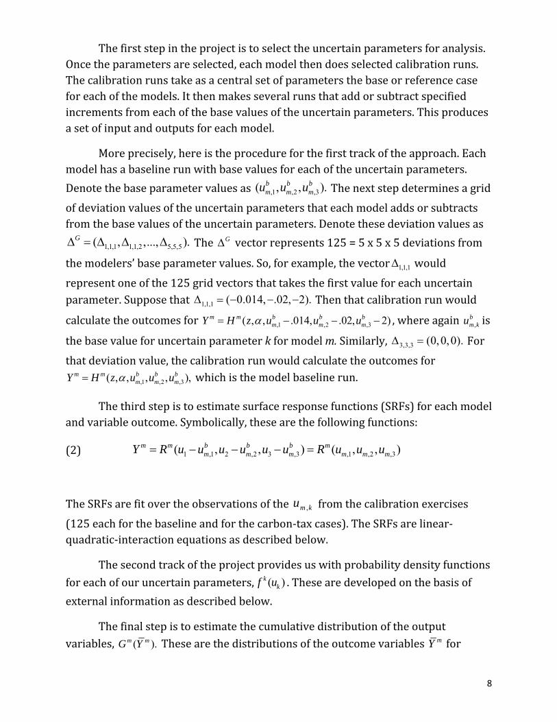
Thefirststepintheprojectistoselecttheuncertainparametersforanalysis.Oncetheparametersareselected,eachmodelthendoesselectedcalibrationruns.Thecalibrationrunstakeasacentralsetofparametersthebaseorreferencecaseforeachofthemodels.Itthenmakesseveralrunsthataddorsubtractspecifiedincrementsfromeachofthebasevaluesoftheuncertainparameters.Thisproducesasetofinputandoutputsforeachmodel.
Moreprecisely,hereistheprocedureforthefirsttrackoftheapproach.Eachmodelhasabaselinerunwithbasevaluesforeachoftheuncertainparameters.
Denotethebaseparametervaluesas ,1 ,2 ,3( , , ).b b bm m mu u u Thenextstepdeterminesagrid
ofdeviationvaluesoftheuncertainparametersthateachmodeladdsorsubtractsfromthebasevaluesoftheuncertainparameters.Denotethesedeviationvaluesas
1,1,1 1,1,2 5,5,5( , ,..., ).G The G vectorrepresents125=5x5x5deviationsfrom
themodelers’baseparametervalues.So,forexample,thevector 1,1,1 would
representoneofthe125gridvectorsthattakesthefirstvalueforeachuncertainparameter.Supposethat 1,1,1 ( 0.014, .02, 2). Thenthatcalibrationrunwould
calculatetheoutcomesfor ,1 ,2 ,3( , , .014, .02, 2)m m b b bm m mY H z u u u ,whereagain ,
bm ku is
thebasevalueforuncertainparameterkformodelm.Similarly, 3,3,3 (0,0,0). For
thatdeviationvalue,thecalibrationrunwouldcalculatetheoutcomesfor
,1 ,2 ,3( , , , , ),m m b b bm m mY H z u u u whichisthemodelbaselinerun.
Thethirdstepistoestimatesurfaceresponsefunctions(SRFs)foreachmodelandvariableoutcome.Symbolically,thesearethefollowingfunctions:
(2) 1 ,1 2 ,2 3 ,3 ,1 ,2 ,3( , , ) ( , , )m m b b b mm m m m m mY R u u u u u u R u u u
TheSRFsarefitovertheobservationsofthe ,m ku fromthecalibrationexercises
(125eachforthebaselineandforthecarbon‐taxcases).TheSRFsarelinear‐quadratic‐interactionequationsasdescribedbelow.
Thesecondtrackoftheprojectprovidesuswithprobabilitydensityfunctions
foreachofouruncertainparameters, ( )kkf u .Thesearedevelopedonthebasisof
externalinformationasdescribedbelow.
Thefinalstepistoestimatethecumulativedistributionoftheoutputvariables, ( ).m mG Y Thesearethedistributionsoftheoutcomevariables mY for
9
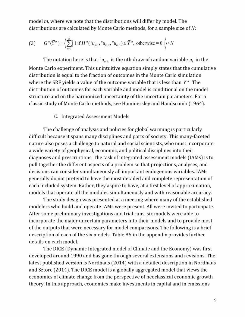
modelm,wherewenotethatthedistributionswilldifferbymodel.ThedistributionsarecalculatedbyMonteCarlomethods,forasamplesizeofN:
(3) ,1 ,2 ,31
( ) 1 if ( , , ) , otherwise = 0 /N
m m m n n n mm m m
n
G Y H u u u Y N
Thenotationhereisthat ,n
m ku isthenthdrawofrandomvariable ku inthe
MonteCarloexperiment.ThisunintuitiveequationsimplystatesthatthecumulativedistributionisequaltothefractionofoutcomesintheMonteCarlosimulationwheretheSRFyieldsavalueoftheoutcomevariablethatislessthan .mY Thedistributionofoutcomesforeachvariableandmodelisconditionalonthemodelstructureandontheharmonizeduncertaintyoftheuncertainparameters.ForaclassicstudyofMonteCarlomethods,seeHammersleyandHandscomb(1964).
C. IntegratedAssessmentModels
Thechallengeofanalysisandpoliciesforglobalwarmingisparticularlydifficultbecauseitspansmanydisciplinesandpartsofsociety.Thismany‐facetednaturealsoposesachallengetonaturalandsocialscientists,whomustincorporateawidevarietyofgeophysical,economic,andpoliticaldisciplinesintotheirdiagnosesandprescriptions.Thetaskofintegratedassessmentmodels(IAMs)istopulltogetherthedifferentaspectsofaproblemsothatprojections,analyses,anddecisionscanconsidersimultaneouslyallimportantendogenousvariables.IAMsgenerallydonotpretendtohavethemostdetailedandcompleterepresentationofeachincludedsystem.Rather,theyaspiretohave,atafirstlevelofapproximation,modelsthatoperateallthemodulessimultaneouslyandwithreasonableaccuracy.
ThestudydesignwaspresentedatameetingwheremanyoftheestablishedmodelerswhobuildandoperateIAMswerepresent.Allwereinvitedtoparticipate.Aftersomepreliminaryinvestigationsandtrialruns,sixmodelswereabletoincorporatethemajoruncertainparametersintotheirmodelsandtoprovidemostoftheoutputsthatwerenecessaryformodelcomparisons.Thefollowingisabriefdescriptionofeachofthesixmodels.TableA5intheappendixprovidesfurtherdetailsoneachmodel.
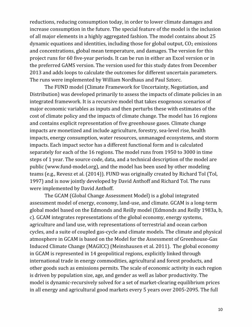
TheDICE(DynamicIntegratedmodelofClimateandtheEconomy)wasfirstdevelopedaround1990andhasgonethroughseveralextensionsandrevisions.ThelatestpublishedversionisNordhaus(2014)withadetaileddescriptioninNordhausandSztorc(2014).TheDICEmodelisagloballyaggregatedmodelthatviewstheeconomicsofclimatechangefromtheperspectiveofneoclassicaleconomicgrowththeory.Inthisapproach,economiesmakeinvestmentsincapitalandinemissions
10
reductions,reducingconsumptiontoday,inordertolowerclimatedamagesandincreaseconsumptioninthefuture.Thespecialfeatureofthemodelistheinclusionofallmajorelementsinahighlyaggregatedfashion.Themodelcontainsabout25dynamicequationsandidentities,includingthoseforglobaloutput,CO2emissionsandconcentrations,globalmeantemperature,anddamages.Theversionforthisprojectrunsfor60five‐yearperiods.ItcanberunineitheranExcelversionorinthepreferredGAMSversion.TheversionusedforthisstudydatesfromDecember2013andaddsloopstocalculatetheoutcomesfordifferentuncertainparameters.TherunswereimplementedbyWilliamNordhausandPaulSztorc.
TheFUNDmodel(ClimateFrameworkforUncertainty,Negotiation,andDistribution)wasdevelopedprimarilytoassesstheimpactsofclimatepoliciesinanintegratedframework.Itisarecursivemodelthattakesexogenousscenariosofmajoreconomicvariablesasinputsandthenperturbsthesewithestimatesofthecostofclimatepolicyandtheimpactsofclimatechange.Themodelhas16regionsandcontainsexplicitrepresentationoffivegreenhousegases.Climatechangeimpactsaremonetizedandincludeagriculture,forestry,sea‐levelrise,healthimpacts,energyconsumption,waterresources,unmanagedecosystems,andstormimpacts.Eachimpactsectorhasadifferentfunctionalformandiscalculatedseparatelyforeachofthe16regions.Themodelrunsfrom1950to3000intimestepsof1year.Thesourcecode,data,andatechnicaldescriptionofthemodelarepublic(www.fund‐model.org),andthemodelhasbeenusedbyothermodelingteams(e.g.,Reveszetal.(2014)).FUNDwasoriginallycreatedbyRichardTol(Tol,1997)andisnowjointlydevelopedbyDavidAnthoffandRichardTol.TherunswereimplementedbyDavidAnthoff.
TheGCAM(GlobalChangeAssessmentModel)isaglobalintegratedassessmentmodelofenergy,economy,land‐use,andclimate.GCAMisalong‐termglobalmodelbasedontheEdmondsandReillymodel(EdmondsandReilly1983a,b,c).GCAMintegratesrepresentationsoftheglobaleconomy,energysystems,agricultureandlanduse,withrepresentationsofterrestrialandoceancarboncycles,andasuiteofcoupledgas‐cycleandclimatemodels.TheclimateandphysicalatmosphereinGCAMisbasedontheModelfortheAssessmentofGreenhouse‐GasInducedClimateChange(MAGICC)(Meinshausenetal.2011).TheglobaleconomyinGCAMisrepresentedin14geopoliticalregions,explicitlylinkedthroughinternationaltradeinenergycommodities,agriculturalandforestproducts,andothergoodssuchasemissionspermits.Thescaleofeconomicactivityineachregionisdrivenbypopulationsize,age,andgenderaswellaslaborproductivity.Themodelisdynamic‐recursivelysolvedforasetofmarket‐clearingequilibriumpricesinallenergyandagriculturalgoodmarketsevery5yearsover2005‐2095.Thefull
11
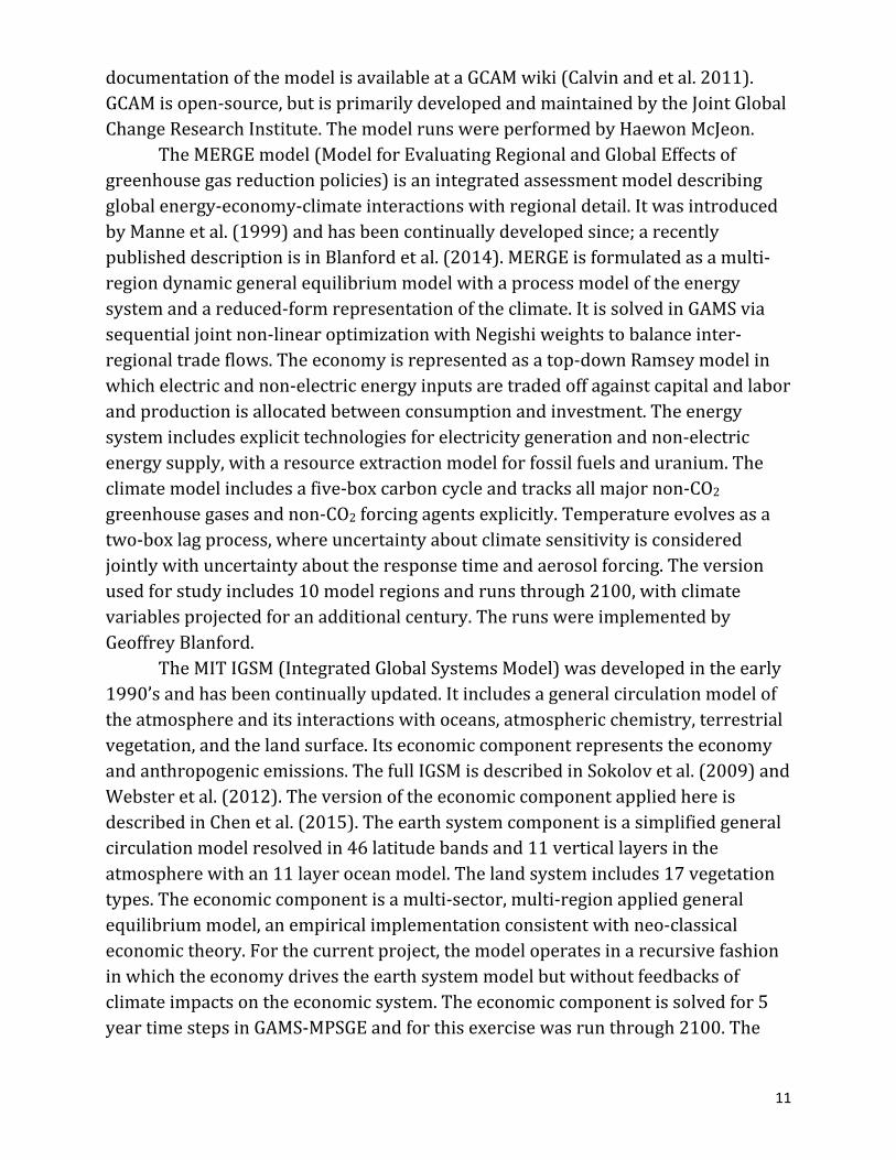
documentationofthemodelisavailableataGCAMwiki(Calvinandetal.2011).GCAMisopen‐source,butisprimarilydevelopedandmaintainedbytheJointGlobalChangeResearchInstitute.ThemodelrunswereperformedbyHaewonMcJeon.
TheMERGEmodel(ModelforEvaluatingRegionalandGlobalEffectsofgreenhousegasreductionpolicies)isanintegratedassessmentmodeldescribingglobalenergy‐economy‐climateinteractionswithregionaldetail.ItwasintroducedbyManneetal.(1999)andhasbeencontinuallydevelopedsince;arecentlypublisheddescriptionisinBlanfordetal.(2014).MERGEisformulatedasamulti‐regiondynamicgeneralequilibriummodelwithaprocessmodeloftheenergysystemandareduced‐formrepresentationoftheclimate.ItissolvedinGAMSviasequentialjointnon‐linearoptimizationwithNegishiweightstobalanceinter‐regionaltradeflows.Theeconomyisrepresentedasatop‐downRamseymodelinwhichelectricandnon‐electricenergyinputsaretradedoffagainstcapitalandlaborandproductionisallocatedbetweenconsumptionandinvestment.Theenergysystemincludesexplicittechnologiesforelectricitygenerationandnon‐electricenergysupply,witharesourceextractionmodelforfossilfuelsanduranium.Theclimatemodelincludesafive‐boxcarboncycleandtracksallmajornon‐CO2greenhousegasesandnon‐CO2forcingagentsexplicitly.Temperatureevolvesasatwo‐boxlagprocess,whereuncertaintyaboutclimatesensitivityisconsideredjointlywithuncertaintyabouttheresponsetimeandaerosolforcing.Theversionusedforstudyincludes10modelregionsandrunsthrough2100,withclimatevariablesprojectedforanadditionalcentury.TherunswereimplementedbyGeoffreyBlanford.
TheMITIGSM(IntegratedGlobalSystemsModel)wasdevelopedintheearly1990’sandhasbeencontinuallyupdated.Itincludesageneralcirculationmodeloftheatmosphereanditsinteractionswithoceans,atmosphericchemistry,terrestrialvegetation,andthelandsurface.Itseconomiccomponentrepresentstheeconomyandanthropogenicemissions.ThefullIGSMisdescribedinSokolovetal.(2009)andWebsteretal.(2012).TheversionoftheeconomiccomponentappliedhereisdescribedinChenetal.(2015).Theearthsystemcomponentisasimplifiedgeneralcirculationmodelresolvedin46latitudebandsand11verticallayersintheatmospherewithan11layeroceanmodel.Thelandsystemincludes17vegetationtypes.Theeconomiccomponentisamulti‐sector,multi‐regionappliedgeneralequilibriummodel,anempiricalimplementationconsistentwithneo‐classicaleconomictheory.Forthecurrentproject,themodeloperatesinarecursivefashioninwhichtheeconomydrivestheearthsystemmodelbutwithoutfeedbacksofclimateimpactsontheeconomicsystem.Theeconomiccomponentissolvedfor5yeartimestepsinGAMS‐MPSGEandforthisexercisewasrunthrough2100.The
12
earthsystemcomponentsolveson10minutetimesteps(thevegetationmodelonmonthlytimesteps).ThesimulationsforthisexercisewereconductedbyY.‐H.HenryChen,AndreiSokolov,andJohnReilly.
TheWITCH(WorldInducedTechnicalChangeHybrid)modelwasdevelopedin2006(Bosettietal.2006)andhasbeendevelopedandextendedsincethen.ThelatestversionisfullydescribedinBosettietal.(2014).Themodeldividestheworldinto13majorregions.TheeconomyofeachregionisdescribedbyaRamsey‐typeneoclassicaloptimalgrowthmodel,whereforward‐lookingcentralplannersmaximizethepresentdiscountedvalueofutilityofeachregion.Theseoptimizationstakeaccountofotherregions'intertemporalstrategies.Theoptimalinvestmentstrategyincludesadetailedappraisalofenergysectorinvestmentsinpower‐generationtechnologiesandinnovation,andthedirectconsumptionoffuels,aswellasabatementofothergasesandland‐useemissions.Greenhouse‐gasemissionsandconcentrationsarethenusedasinputsinaclimatemodelofreducedcomplexity(Meinshausenetal.2011).Theversionusedforthisprojectrunsfor30five‐yearperiodsandcontains35statevariablesforeachofthe13regions,runningontheGAMSplatform.TherunswereimplementedbyValentinaBosettiandGiacomoMarangoni.
IV. Choiceofuncertainparametersandgriddesign
A. Choiceofuncertainparameters
Oneofthekeydecisionsinthisstudywastoselecttheuncertainparameters.Thecriteriaforselectionwere(atleastafterthefact)clear.First,eachparametermustbeimportantforinfluencinguncertainty.Second,parametersshouldbeonesthatcanbevariedineachofthemodelswithoutexcessiveburdenandwithoutviolatingthespiritofthemodelstructure.Third,theparametersshouldbeonesthatcanberepresentedbyaprobabilitydistribution,eitheronthebasisofpriorresearchorfeasiblewithinthescopeofthisproject. Ataninitialmeeting,anexperimentwasundertakeninwhicheachofthemodelswasgivensixuncertainparametersorshockstotestforfeasibility.Attheendofthisinitialtestexperiment,twoofthemodelingteamsdecidednottoparticipatebecausetheinitialparameterscouldnotbeeasilyincorporatedinthemodeldesignorbecauseoftimeconstraints.Threeoftheparametersfulfilledtheabove‐mentionedcriteria,andtheseweretheonesthatwereincorporatedinthefinalsetofexperiments. Thefinallistofuncertainparameterswerethefollowing:(1)Therateofgrowthofproductivity,orpercapitaoutput;(2)therateofgrowthofpopulation;
13
and(3)theequilibriumclimatesensitivity(equilibriumchangeinglobalmeansurfacetemperaturefromadoublingofatmosphericCO2concentrations).
Additionally,itwasdecidedtodotwoalternativepolicyscenarios.Onewasa“Base”runinwhichnoclimatepolicieswereintroduced;andthesecond,labelled“CarbonTax”(andsometimes“Ampere”)introducedarapidlyrisingglobalcarbontax.2Arunbasedoncarbonpriceswasselected(insteadofquantitativelimits)becausemanymodelshadundertakensimilarrunsinothermodelcomparisonprojects,sotheywererelativelyeasytoimplement.
Severalotherparameterswerecarefullyconsideredbutrejected.Apulseofemissionswasrejectedbecauseithadessentiallynoimpact.Aglobalrecessionwasrejectedforthesamereason.Itwashopedtoadduncertaintiesfortechnology(suchasthoseconcerningtherateofdecarbonization,thecostofbackstoptechnologies,orthecostofadvancedcarbon‐freetechnologies),butitprovedimpossibletofindonethatwasbothsufficientlycomprehensiveandcouldbeincorporatedinallthemodels.Uncertaintyaboutclimatedamageswasexcludedbecausehalfthemodelsdidnotcontaindamages.Afinalpossibilitywastoanalyzepolicyrunsthathadquantitativelimitsratherthancarbonprices.Forexample,somemodelshadparticipatedinmodelcomparisonsinwhichradiativeforcingswerelimited.Thisapproachwasrejectedbecausethecarbontaxprovedeasiertodefineandimplement.Additionally,earlierexperimentsindicatedthatquantitativelimitswereoftenfoundinfeasible,andthiswouldcloudtheinterpretationoftheresults.3
2TheCarbonTaxrunwasselectedfromtheAMPEREmodelcomparisonstoreducetheburdenonmanyofthemodelersandsothattheresultsfromthisstudycanbecomparedtothosefromtheAMPEREinter‐modelcomparisonstudy(Kriegleretal.2015).ThespecificscenariochosenisknownintheAMPEREstudyas"CarbonTax$12.50‐increasing.”ThefullAMPEREscenariodatabasecanbefoundonlineathttps://secure.iiasa.ac.at/web‐apps/ene/AMPEREDB.3SeeparticularlytheresultsforEnergyModelingForum22reportedinaspecialissueinEnergyEconomics(e.g.,seeClarkeandWeyant(2009)).Manymodelsfoundthattightconstraintswereinfeasiblefortheirbaseruns.Aquantitativelimitwouldalmostsurelyhavefoundthatlargenumbersofthe125scenarioswereinfeasibleforanytightlimitontemperatureorradiativeforcings.
14
B. Descriptionofuncertainparameters
Wenextdescribethethreeuncertainparameterscontainedinthestudy.Itturnedoutthatharmonizingtheseacrossmodelswasmorecomplicatedthanwasoriginallyanticipated,asdescribedbelow.
(1) Therateofgrowthofpopulation.Uncertaintyabouttherateofgrowthofpopulationwasstraightforward.Forglobalmodels,therewasnoambiguityabouttheadjustment.Theuncertaintywasspecifiedasplusorminusauniformpercentagegrowthrateeachyearovertheperiod2010‐2100.Forregionalmodels,theadjustmentwaslefttothemodeler.Mostmodelsassumedauniformchangeinthegrowthrateineachregion.
(2)Therateofgrowthofproductivity,orpercapitaoutput.Theoriginaldesignhadbeentoincludeavariablethatrepresentedtheuncertaintyaboutoveralltechnologicalchangeintheglobaleconomy(oraveragedacrossregions).Theresultsoftheinitialexperimentindicatedthatthespecificationsoftechnologicalchangedifferedgreatlyacrossmodels,anditwasinfeasibletospecifyacomparabletechnologicalvariablethatcouldapplyforallmodels.Forexample,somemodelshadasingleproductionfunction,whileothershadmultiplesectors.
Ratherthanattempttofindacomparableparameter,itwasdecidedtoharmonizeontheuncertaintyofglobaloutputpercapitagrowthfrom2010to2100.Eachmodelerwasaskedtointroduceagridofchangesinitsmodel‐specifictechnologicalparameterthatwouldleadtoachangeinpercapitaoutputofplusorminusagivenamount(tobedescribedinthenextsection).ThemodelersweretheninstructedtoadjustthatchangesothattherangeofgrowthratesinpercapitaGDPfrom2010to2100inthecalibrationexercisewouldbeequaltothedesiredrange.
(3)Theclimatesensitivity.Modelinguncertaintyaboutclimatesensitivityprovedtobeoneofthemostdifficultissuesofharmonizationacrossthedifferentmodels.WhileallmodelshavemodulestotracethroughthetemperatureimplicationsofchangingconcentrationsofGHGs,theydifferindetailandspecification.Themajorproblemwasthatadjustingtheequilibriumclimatesensitivitygenerallyrequiredadjustingotherparametersinthemodelthatdeterminethespeedofadjustmenttotheequilibrium;theadjustmentspeedissometimesrepresentedbythetransientclimatesensitivity.Thisproblemwasidentifiedlateintheprocess,afterthesecond‐roundrunshadbeencompleted,andmodelerswereaskedtomaketheadjustmentsthattheythoughtappropriate.Somemodelsmadeadjustmentsinparameterstoreflectdifferencesinlargeclimate
15
models.Othersconstrainedtheparameterssothatthemodelwouldfitthehistoricaltemperaturerecord.Thedifferingapproachesledtodifferingstructuralresponsestotheclimatesensitivityuncertainty,aswillbeseenbelow.
C. Griddesign
Inthefirsttrack,themodelingteamsprovideasmallnumberofcalibrationrunsthatincludeafullsetofoutputsforathree‐dimensionalgridofvaluesoftheuncertainparameters.Foreachoftheuncertainparameters,weselectedfivevaluescenteredonthemodel’sbaselinevalues.Therefore,for3uncertainparameters,therewere125runseachfortheBaseandtheCarbonTaxpolicyscenarios.
Onthebasisofthesecalibrationruns,thenextstepinvolvedestimatingsurface‐responsefunctions(SRFs)inwhichthemodeloutcomesareestimatedasfunctionsoftheuncertainparameters.ThehopewasthatiftheSRFscouldapproximatethemodelsaccurately,thentheycouldbeusedtosimulatetheprobabilitydistributionsoftheoutcomevariablesaccurately.AninitialtestsuggestedthattheSRFswerewellapproximatedbyquadraticfunctions.Wethereforesettherangeofthegridsothatitwouldspanmostofthespacethatwouldbecoveredbythedistributionoftheuncertainparameters,yetnotgosofarastopushthemodelsintopartsoftheparameterspacewheretheresultswouldbeunreliable.
Asanexample,takethegridforpopulationgrowth.Thecentralcaseisthemodel’sbasecaseforpopulationgrowth.Eachmodelthenusesfouradditionalassumptionsforthegridforpopulationgrowth:thebasecaseplusandminus0.5%peryearandplusandminus1.0%peryear.Thesewouldcovertheperiod2010to2100.Forexample,assumethatthemodelhadabasecasewithaconstantpopulationgrowthrateof0.7%peryearfrom2010to2100.Thenthefivegridpointsforpopulationgrowthwouldbeconstantgrowthratesof‐0.3%,0.2%,0.7%,1.2%,and1.7%peryear.Populationafter2100wouldhavethesamegrowthrateasinthemodeler’sbasecase.Theseassumptionsmeanthatpopulationin2100wouldbe(0.99)90,(0.995)90,1,(1.005)90,and(1.01)90timesthebasecasepopulationfor2100.
Forproductivitygrowth,thegridwassimilarlyconstructed,butadjustedsothatthegrowthinpercapitaoutputfor2100added‐1%,‐0.5%,0%,0.5%,and1%tothegrowthrateineachyearfortheperiod2010‐2100.
Fortheclimatesensitivity,themodelersweretoaddtothebaselineequilibriumclimatesensitivity‐3°C,‐1.5°C,0°C,1.5°C,and3°C.Itturnedoutthatthelowerendofthisrangecauseddifficultiesforsomemodels,andforthesethe
16
modelersreportedresultsonlyforthefourhigherpointsinthegridorsubstitutedanotherlowvalue.
Inprinciple,then,fortrackIeachmodelreported5x5x5modelresultsforboththeBasecaseandtheCarbonTaxpolicyassumptions.
V. Approachfordevelopingprobabilitydensityfunctions
A. Generalconsiderations
Thethreeuncertainparametershavebeenthesubjectofuncertaintyanalysisinearlierstudies.Foreachparameter,wereviewedearlierstudiestodeterminewhethertherewasanexistingsetofmethodsordistributionsthatcouldbedrawnupon.Thedesirablefeaturesofthedistributionsisthattheyshouldreflectbestpractice,thattheyshouldbeacceptabletothemodelinggroups,andthattheybereplicable.Itturnedoutthatthethreeparametersusedthreedifferentapproaches,aswillbedescribedbelow.
B. Population
Populationgrowthhasbeenthesubjectofprojectionsformanyyears,andnumerousgroupshaveundertakenuncertaintyanalysesforbothcountriesandatthegloballevel.Ourreviewfoundonlyoneresearchgroupthathadmadelong‐termglobalprojectionsofuncertaintyforseveralyears,whichwasthepopulationgroupattheInternationalInstituteforAppliedSystemsAnalysis(IIASA)inAustria.(Foradiscussion,seeO'Neilletal.(2001)).TheIIASAdemographygroupisunderthedirectionofdemographerWolfgangLutz.
TheIIASAstochasticprojectionsweredevelopedoveraperiodofmorethanadecadeandarewidelyusedbydemographers.Themethodologyissummarizedasfollows:“IIASA’sprojections…arebasedexplicitlyontheresultsofdiscussionsofagroupofexpertsonfertility,mortality,andmigrationthatisconvenedforthepurposeofproducingscenariosforthesevitalrates”(Seehttp://www.demographic‐research.org/volumes/vol4/8/4‐8.pdf)Thelatestprojectionsfrom2013(Lutzetal.2014)areanupdatetothepreviousprojectionsfrom2007and2001(Lutzetal.2008),2001).Themethodologyisdescribedasfollows:
Theforecastsarecarriedoutfor13worldregions.Theforecastspresentedherearenotalternativescenariosorvariants,butthedistributionoftheresultsof2,000differentcohortcomponentprojections.Forthesestochasticsimulationsthefertility,mortalityandmigrationpathsunderlyingtheindividualprojection
17
runswerederivedrandomlyfromthedescribeduncertaintydistributionforfertility,mortalityandmigrationinthedifferentworldregions.(Lutz,Sanderson,andScherbov2008)
Thebackgroundmethodsaredescribedasfollowsonpage219ofO'Neilletal.(2001):
TheIIASAmethodologyisbasedonaskingagroupofinteractingexpertstogivealikelyrangeforfuturevitalrates,where"likely"isdefinedtobeaconfidenceintervalofroughly90%(Lutz1996,Lutzetal.1998).Combiningsubjectiveprobabilitydistributionsfromanumberofexpertsguardsagainstindividualbias,andIIASAdemographersarguethatastrengthofthemethodisthatitmaybepossibletocapturestructuralchangeandunexpectedeventsthatotherapproachesmightmiss.Inaddition,inareaswheredataonhistoricaltrendsaresparse,theremaybenobetteralternativetoproducingprobabilisticprojections.
Forthisstudy,weareaimingforaparsimoniousparameterizationofpopulationuncertainty.Thisisnecessarybecauseofthelargedifferencesinmodelstructure.Wethereforeselectedtheuncertaintyaboutglobalpopulationgrowthfortheperiod2010‐2100asthesingleparameterofinterest.Wefittedthegrowth‐ratequantilesfromtheIIASAprojectionstoseveraldistributions,withnormal,log‐normal,andgammabeingthemostsatisfactory.Thenormaldistributionperformedbetterthananyoftheothersonfiveofthesixquantitativetestsoffitfordistributions.Basedontheseresults,wethereforedecidedtorecommendthenormaldistributionforthepdfofpopulationgrowthovertheperiod.
Inaddition,wedidseveralalternativeteststodeterminewhethertheprojectionswereconsistentwithothermethodologies.Onesetoftestsexaminestheprojectionerrorsthatwouldhavebeengeneratedusinghistoricaldata.Asecondtestlooksatthestandarddeviationof100‐yeargrowthratesofpopulationforthelastmillennium.AthirdtestexaminesprojectionsfromareportoftheNationalResearchCouncilthatestimatedtheforecasterrorsforglobalpopulationovera50‐yearhorizon(seeNRC(2000),AppendixF,p.344).Whiletheseallgaveslightlydifferentuncertaintyranges,theyweresimilartotheuncertaintiesestimatedintheIIASAstudy.
Onthebasisofthisreview,wedecidedtouseanormaldistributionforthegrowthrateofpopulationbasedontheIIASAstudythathasastandarddeviationoftheaverageannualgrowthrateof0.22percentagepointsperyearovertheperiod
18
2010‐2100.Moredetailswithabackgroundmemorandumontheresultsareavailablefromtheauthors.
C. ClimateSensitivity
Animportantparameterinclimatescienceistheequilibriumorlong‐runresponseintheglobalmeansurfacetemperaturetoadoublingofatmosphericcarbondioxide.Intheclimatesciencecommunity,thisiscalledtheequilibriumclimatesensitivity.Withreferencetoclimatemodels,thisiscalculatedastheincreaseinaveragesurfacetemperaturewithadoubledCO2concentrationrelativetoapathwiththepre‐industrialCO2concentration.ThisparameteralsoplaysakeyroleinthegeophysicalcomponentsintheIAMsusedinthisstudy.Intheremainderofthispaper,wewillfollowtheconventioninthegeosciencesandcallittheequilibriumclimatesensitivity(ECS).
GiventheimportanceoftheECSinclimatescience,thereisanextensiveliteratureestimatingprobabilitydensityfunctions.Thesepdfsaregenerallybasedonclimatemodels,theinstrumentalrecordsoverthelastcenturyorso,paleoclimaticdatasuchasestimatedtemperatureandradiativeforcingsoverice‐ageintervals,andtheresultsofvolcaniceruptions.Muchoftheliteratureestimatesaprobabilitydensityfunctionusingasinglelineofevidence,butafewpaperssynthesizedifferentstudiesordifferentkindsofevidence.
Wefocusonthestudiesdrawinguponmultiplelinesofevidence.TheIPCCFifthAssessmentreport(AR5)reviewedtheliteraturequantifyinguncertaintyintheECSandhighlightedfiverecentpapersusingmultiplelinesofevidence(IPCC2014).EachpaperusedaBayesianapproachtoupdateapriordistributionbasedonpreviousevidence(thepriorevidenceusuallydrawnfrominstrumentalrecordsoraclimatemodel)tocalculatetheposteriorprobabilitydensityfunction.Sinceeachdistributionwasdevelopedusingmultiplelinesofevidence,andinsomecasesthesameevidence,itwouldbeinconsistenttoassumethattheywereindependentandsimplytocombinethem.Further,sincewecouldnotreliablyestimatethedegreeofdependenceofthedifferentstudies,wecouldnotsynthesizethembytakingintoaccountthedependence.WethereforechosetheprobabilitydensityfunctionfromasinglestudyandperformedrobustnesscheckstousingtheresultsfromalternativestudiescitedintheIPCCAR5.
ThechosenstudyforourprimaryestimatesisOlsenetal.(2012).ThisstudyisrepresentativeoftheliteratureinusingaBayesianapproach,withapriorbasedonpreviousstudiesandalikelihoodbasedonobservationalormodeleddata,suchasglobalaveragesurfacetemperaturesorglobaltotalheatcontent.ThepriorinOlsenetal.(2012)isprimarilybasedonKnuttiandHegerl(2008).Thatprioristhen
19
combinedwithoutputvariablesfromtheUniversityofVictoriaESCMclimatemodel(Weaveretal.2001)todeterminethefinalorposteriordistribution.
Olsenetal.(2012)waschosenforthefollowingreasons.First,itwasrecommendedtousinpersonalcommunicationswithseveralclimatescientists.Second,itwasrepresentativeoftheotherfourstudiesweexaminedandfallsintothemiddlerangeofthedifferentestimates.4Third,sensitivityanalysesoftheeffectonaggregateuncertaintyofchangingthestandarddeviationoftheOlsenetal.(2012)resultsfoundthatthesensitivitywassmall(seethesectionbelowonsensitivityanalyses).Appendix1providesmoredetailsonOlsenetal.(2012)andalsopresentsafigurecomparingthisstudytotheotherstudiesintheIPCCAR5.
NotethattheUSgovernmentusedaversionoftheRoeandBakerdistributioncalibratedtothreeconstraintsfromtheIPCCforitsuncertaintyestimates(IAWG2010).Specifically,theIAWGReportmodifiedtheoriginalRoeandBakerdistributiontoassumethatthemedianvalueis3.0°C,theprobabilityofbeingbetween2and4.5°Cistwo‐thirds,andthereisnomassbelowzeroorabove10°C.ThemodifiedRoeandBakerdistributionhasahighermeanECSthananyofthemodels(3.5°C)andamuchhigherdispersion(1.6°Cascomparedto0.84°CfromOlsenetal.2012).
TheestimatedpdfforOlsenetal.(2012)wasderivedasfollows.Wefirstobtainedthepdffromtheauthors.Thispdfwasprovidedasasetofequilibriumtemperaturevaluesandcorrespondingprobabilities.Wethenexploredfamiliesofdistributionsthatbestapproximatedthenumericalpdfprovided.Wefoundthatalog‐normalpdffitstheposteriordistributionsextremelywell.
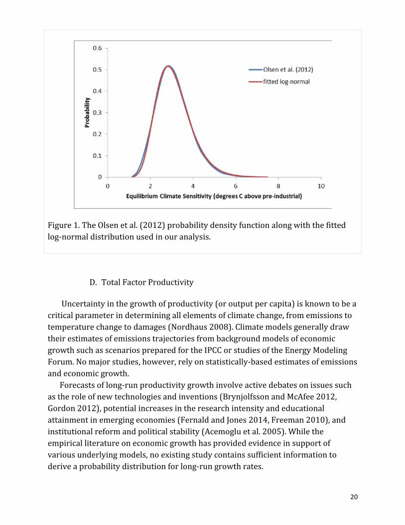
Tofindtheparametersofthefittedlog‐normalpdf,weminimizethesquareddifferencebetweentheposteriordensityfunctionfromOlsenetal.andthelog‐normalpdfoverthesupportofthedistribution(theL2orEuclidiannorm).Inotherwords,weminimizethesumofthesquareoftheverticaldifferencesbetweentheposteriorpdfandalog‐normalpdfoverallgridpointsvaluesintheOlsenetal.(2012)distribution.5Figure1showstheOlsenetal.(2012)pdf,alongwiththefittedlog‐normaldensityfunction.Thefitisextremelyclose,withthelog‐normaldistributionalwayswithin0.14%oftheOlsenetal.(2012)pdfforanygridpointvalue.
4Intests,wefoundthattheOlsenetal.(2012)distributionissimilartoasimplemixturedistributionofallfivedistributions.Wecalculatethismixturedistributionbytakingtheaverageprobabilityoveralldistributionsateachtemperatureincrease.5MorepreciselyweminimizeovertherangeoftheOlsenetal.distribution,[1.509,7.4876]°C,withagridpointspacingof0.1508°C.
20
D. TotalFactorProductivity
Uncertaintyinthegrowthofproductivity(oroutputpercapita)isknowntobeacriticalparameterindeterminingallelementsofclimatechange,fromemissionstotemperaturechangetodamages(Nordhaus2008).ClimatemodelsgenerallydrawtheirestimatesofemissionstrajectoriesfrombackgroundmodelsofeconomicgrowthsuchasscenariospreparedfortheIPCCorstudiesoftheEnergyModelingForum.Nomajorstudies,however,relyonstatistically‐basedestimatesofemissionsandeconomicgrowth.
Forecastsoflong‐runproductivitygrowthinvolveactivedebatesonissuessuchastheroleofnewtechnologiesandinventions(BrynjolfssonandMcAfee2012,Gordon2012),potentialincreasesintheresearchintensityandeducationalattainmentinemergingeconomies(FernaldandJones2014,Freeman2010),andinstitutionalreformandpoliticalstability(Acemogluetal.2005).Whiletheempiricalliteratureoneconomicgrowthhasprovidedevidenceinsupportofvariousunderlyingmodels,noexistingstudycontainssufficientinformationtoderiveaprobabilitydistributionforlong‐rungrowthrates.
Figure1.TheOlsenetal.(2012)probabilitydensityfunctionalongwiththefittedlog‐normaldistributionusedinouranalysis.
21
Thehistoricalrecordprovidesausefulbackgroundforestimatingfuturetrends.However,itisclearfromboththeoreticalandempiricalperspectivesthattheprocessesdrivingproductivitygrowtharenon‐stationary.Forexample,estimatesofthegrowthofglobaloutputpercapitaforthe18th,19th,and20thcenturyare0.6,1.9,and3.7percentperyear(DeLong2015inhttp://holtz.org/Library/Social%20Science/Economics/Estimating%20World%20GDP%20by%20DeLong/Estimating%20World%20GDP.htm).Totheextentthatexpertsoneconomicgrowthpossessvalidinsightsaboutthelikelihoodandpossibledeterminantsoflong‐rungrowthpatterns,theninformationdrawnfromexpertscanaddvaluetoforecastsbasedpurelyonhistoricalobservationsordrawnfromasinglemodel.Combiningexpertestimateshasbeenshowntoreduceerrorinshort‐runforecastsofeconomicgrowth(BatchelorandDua1995).However,therearefewexpertstudiesonlong‐rungrowth(seeAppendix2fordiscussion)and,toourknowledge,therehasbeennosystematicanddetailedpublishedstudyofuncertaintyinlong‐runfuturegrowthrates.
Todevelopestimatesofuncertainties,theprojectteam,ledbyPeterChristensen,undertookasurveyofexpertsoneconomicgrowthtodetermineboththecentraltendencyandtheuncertaintyaboutlong‐rungrowthtrends.Oursurveyutilizedinformationdrawnfromapanelofexpertstocharacterizeuncertaintyinestimatesofglobaloutputfortheperiods2010‐2050and2010‐2100.WedefinedgrowthastheaverageannualrateofrealpercapitaGDP,measuredinpurchasingpowerparity(PPP)terms.Weaskedexpertstoprovideestimatesoftheaverageannualgrowthratesat10th,25th,50th,75th,90thpercentiles.
Beginninginthesummerof2014,wesentoutsurveystoapanelof25economicgrowthexperts.AsofJune2015,wecollected11completeresultswithfulluncertaintyanalysisfortheperiod2010‐2100.AsummaryoftheprocedureisprovidedinAppendix2,andacompletereportwillbepreparedseparately.
Therearemanydifferentapproachestocombiningexpertforecasts(Armstrong2001)andaggregatingprobabilitydistributions(ClemenandWinkler1999).Weassumethatexpertshaveinformationaboutthelikelydistributionoflong‐rungrowthrates.Theirinformationsetsaredefinedbyestimatesfor5differentpercentiles.Webeginbyassumingthattheestimatesareindependentacrossexpertsandthenexaminedthedistributionsthatbestfitthepercentilesforeachexpertandforthecombinedestimates(averageofpercentiles)acrossexperts.
WefounditusefulforthisprojecttocharacterizetheexpertpdfswithcommonlyuseddistributionssothattheMonteCarloestimatescouldbeeasilyimplemented.Intestingthedistributionsforeachexpert,wefoundthatmostexperts’estimatescan
22
becloselyfittedbyanormaldistribution;similarly,thecombineddistributioniswellfittedbyanormaldistribution.DetailsareprovidedinAppendix2.
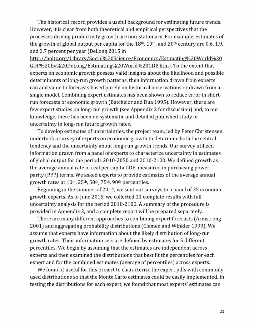
Theresultingcombinednormaldistributionhasameangrowthrateof2.29%peryearandastandarddeviationofthegrowthrateof1.15%peryearovertheperiod2010‐2100.(ThemeangrowthrateofpercapitaGDPinthebaserunsofthesixmodelsisslightlylowerat1.9%peryearoverthisperiod.)Wetestdifferentapproachesforcombiningtheexpertresponsesandfindlittlesensitivitytothechoiceofaggregationmethod.Figure2showsthefittedindividualandcombinednormalpdfs(explainedinAppendix2).IntheMonteCarloestimatesbelow,wechoseastandarddeviationofthegrowthrateofpercapitaoutputof1.12%peryear(basedonthefirst11responses).Thisvalueisusedinthisdraft,butwillbeupdatedwiththeadditionoffurtherresponses.
Figure2.Individualandcombinedpdfsforannualgrowthratesofoutputpercapita,2010–2100(averageannualpercentperyear)Forthemethods,seeAppendix2.
23
Itisusefultocomparethesurveyresultswithhistoricaldata.Ifwetakethelong‐termestimatesfromMaddison(2003),the100‐yearvariabilityofgrowthoverthetencenturiesfrom1000to2000was1.5%peryear,witharangeof‐0.1%to3.7%peryear.Thevariabilityinthesecentury‐stepdataishigherthantheexperts’estimateof1.15%peryear.
Globalgrowthratesbasedondetailednationaldataareavailablesince1900.Thestandarddeviationofannualgrowthratesoverthisperiodwas2.9%peryear,whilethestandarddeviationof25‐yeargrowthrateswas1.2or1.4%peryeardependinguponthesource.Thevariabilityofgrowthinrecentyearswaslowerthanfortheentireperiodsince1900.Thestandarddeviationintheannualgrowthrateduringtheperiod1975‐2000was1.1%peryear.Wecannoteasilytranslatehistoricalvariabilitiesintocentury‐longvariabilitieswithoutassumingaspecificstochasticstructureofgrowthrates.
VI. ResultsofModelingStudies
A. Modelresultsandlatticediagrams
Webeginbyprovidingresultsonthecalibrationrunsandthesurfaceresponsefunctions.Foreachmodel,thereisavoluminoussetofinputsandoutputvariablesfrom2010to2100.Thefullset(consistingof46,150x22elements)clearlycannotbefullypresented.Werestrictourfocusheretosomeofthemostimportantresults,andconsignfurtherresultstoAppendix3,withthefullresultsavailableonlineattimeofpublication.
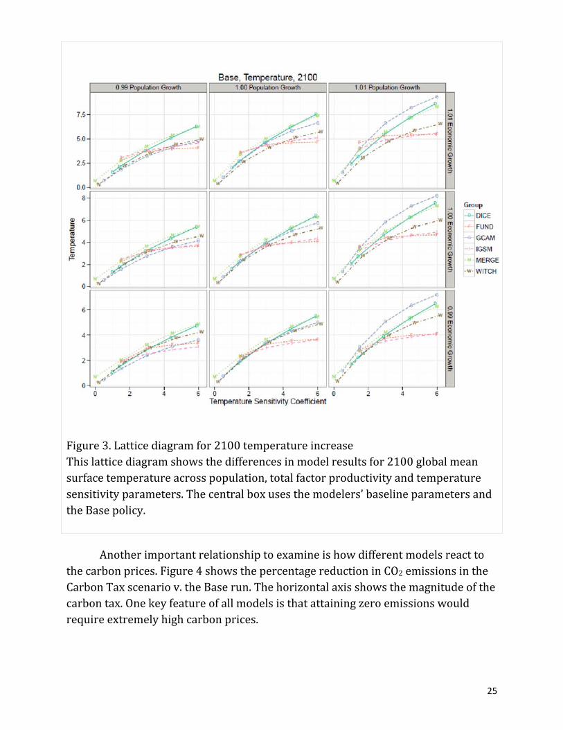
Tohelpvisualizetheresults,wehavedevelopedlatticediagramstoshowhowtheresultsvaryacrossuncertainvariablesandmodels.Figure3isalatticediagramfortheincreaseinglobalmeansurfacetemperaturein2100.Withineachoftheninepanels,they‐axisistheglobalmeansurfacetemperatureincreasein2100relativeto1900.Thex‐axisisthevalueoftheequilibriumtemperaturesensitivity.Goingacrosspanelsonthehorizontalaxis,thefirstcolumnusesthegridvalueofthefirstofthefivepopulationscenarios(whichisthelowestgrowthrate);themiddlecolumnshowstheresultsforthemodeler’sbaselinepopulation;andthethirdcolumnshowstheresultsforthepopulationassociatedwiththehighestpopulationgrid(orhighestgrowthrate).
Goingdownpanelsontheverticalaxis,thefirstrowusesthehighestgrowthrateforTFP(orthefifthTFPgridpoint);themiddlerowshowsTFPgrowthforthemodelers’baselines;andthebottomrowshowstheresultsfortheslowestgridpointforthegrowthrateofTFP.Notethatinallcases,themodelers’baselinevalues
24
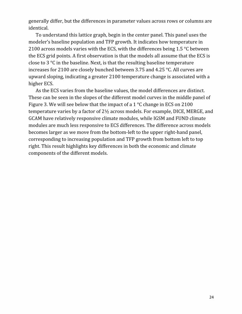
generallydiffer,butthedifferencesinparametervaluesacrossrowsorcolumnsareidentical.
Tounderstandthislatticegraph,begininthecenterpanel.Thispanelusesthemodeler’sbaselinepopulationandTFPgrowth.Itindicateshowtemperaturein2100acrossmodelsvarieswiththeECS,withthedifferencesbeing1.5°CbetweentheECSgridpoints.AfirstobservationisthatthemodelsallassumethattheECSiscloseto3°Cinthebaseline.Next,isthattheresultingbaselinetemperatureincreasesfor2100arecloselybunchedbetween3.75and4.25°C.Allcurvesareupwardsloping,indicatingagreater2100temperaturechangeisassociatedwithahigherECS.
AstheECSvariesfromthebaselinevalues,themodeldifferencesaredistinct.ThesecanbeseenintheslopesofthedifferentmodelcurvesinthemiddlepanelofFigure3.Wewillseebelowthattheimpactofa1°CchangeinECSon2100temperaturevariesbyafactorof2½acrossmodels.Forexample,DICE,MERGE,andGCAMhaverelativelyresponsiveclimatemodules,whileIGSMandFUNDclimatemodulesaremuchlessresponsivetoECSdifferences.Thedifferenceacrossmodelsbecomeslargeraswemovefromthebottom‐lefttotheupperright‐handpanel,correspondingtoincreasingpopulationandTFPgrowthfrombottomlefttotopright.Thisresulthighlightskeydifferencesinboththeeconomicandclimatecomponentsofthedifferentmodels.
25
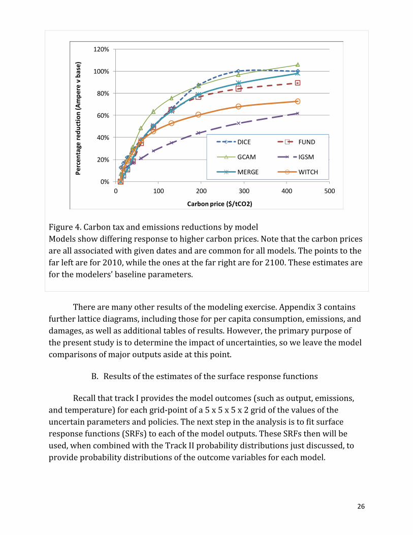
Anotherimportantrelationshiptoexamineishowdifferentmodelsreacttothecarbonprices.Figure4showsthepercentagereductioninCO2emissionsintheCarbonTaxscenariov.theBaserun.Thehorizontalaxisshowsthemagnitudeofthecarbontax.Onekeyfeatureofallmodelsisthatattainingzeroemissionswouldrequireextremelyhighcarbonprices.
Figure3.Latticediagramfor2100temperatureincreaseThislatticediagramshowsthedifferencesinmodelresultsfor2100globalmeansurfacetemperatureacrosspopulation,totalfactorproductivityandtemperaturesensitivityparameters.Thecentralboxusesthemodelers’baselineparametersandtheBasepolicy.
26
Therearemanyotherresultsofthemodelingexercise.Appendix3containsfurtherlatticediagrams,includingthoseforpercapitaconsumption,emissions,anddamages,aswellasadditionaltablesofresults.However,theprimarypurposeofthepresentstudyistodeterminetheimpactofuncertainties,soweleavethemodelcomparisonsofmajoroutputsasideatthispoint.
B. Resultsoftheestimatesofthesurfaceresponsefunctions
RecallthattrackIprovidesthemodeloutcomes(suchasoutput,emissions,andtemperature)foreachgrid‐pointofa5x5x5x2gridofthevaluesoftheuncertainparametersandpolicies.Thenextstepintheanalysisistofitsurfaceresponsefunctions(SRFs)toeachofthemodeloutputs.TheseSRFsthenwillbeused,whencombinedwiththeTrackIIprobabilitydistributionsjustdiscussed,toprovideprobabilitydistributionsoftheoutcomevariablesforeachmodel.
Figure4.CarbontaxandemissionsreductionsbymodelModelsshowdifferingresponsetohighercarbonprices.Notethatthecarbonpricesareallassociatedwithgivendatesandarecommonforallmodels.Thepointstothefarleftarefor2010,whiletheonesatthefarrightarefor2100.Theseestimatesareforthemodelers’baselineparameters.
0%
20%
40%
60%
80%
100%
120%
0 100 200 300 400 500
Percen
tage red
uction (A
mpere v base)
Carbon price ($/tCO2)
DICE FUND
GCAM IGSM
MERGE WITCH
27
WeundertookextensiveanalysisofdifferentapproachestoestimatingtheSRFs.Theinitialandeventuallypreferredapproachwasalinear‐quadratic‐interactions(LQI)specification.Thistookthefollowingform:
3 3
01 1 1
j
i i ij i ji j i
Y u u u
Inthisspecification, and i ju u aretheuncertainparameters.TheYarethe
outcomevariablesfordifferentmodelsanddifferentyears(e.g.,temperaturefortheFUNDmodelfor2100intheBaserunfordifferentvaluesofthe3uncertainparameters).Theparameters 0 , , and i i j aretheestimatesfromtheSRF
regressionequations.Wesuppressthesubscriptforthemodel,year,policy,andvariable.
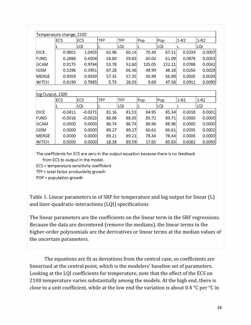
Table1showsacomparisonoftheresultsfortemperatureandlogofoutputforthelinear(L)andLQIspecificationsforthesixmodels.AllspecificationsshowmarkedimprovementoftheequationfitintheLQIrelativetotheLversion.Lookingatthelogoutputspecification(thelastcolumninthebottomsetofnumbers),theresidualvarianceintheLQIspecificationisessentiallyzeroforallmodels.ForthetemperatureSRF,morethan99.5%ofthevarianceisexplainedbytheLQIspecification.Thestandarderrorsofequationsfor2100temperaturerangefrom0.05to0.18°CfordifferentmodelsintheLQIversion.
28
Theequationsarefitasdeviationsfromthecentralcase,socoefficientsarelinearizedatthecentralpoint,whichisthemodelers’baselinesetofparameters.LookingattheLQIcoefficientsfortemperature,notethattheeffectoftheECSon2100temperaturevariessubstantiallyamongthemodels.Atthehighend,thereisclosetoaunitcoefficient,whileatthelowendthevariationisabout0.4°Cper°Cin
Table1.LinearparametersinofSRFfortemperatureandlogoutputforlinear(L)andliner‐quadratic‐interactions(LQI)specifications
ThelinearparametersarethecoefficientsonthelineartermintheSRFregressions.Becausethedataaredecentered(removethemedians),thelineartermsinthehigher‐orderpolynomialsarethederivativesorlineartermsatthemedianvaluesoftheuncertainparameters.
29
ECSchange.ForTFP,theimpactsarerelativelysimilarexceptfortheWITCHmodel,whichismuchlower.ThisislikelyduetoimplementationoftheTFPchangesasinput‐neutraltechnicalchange(ratherthanchangesinlaborproductivity,asinseveralothermodels).Forpopulation,theLQIcoefficientsvarybyafactorofthree.
Forlogofoutput,severalmodelshavenofeedbackfromECStooutputandthusshowa0.000value.TheimpactofTFPisalmostuniformbydesign.Similarly,theimpactofpopulationonoutputisverysimilar.
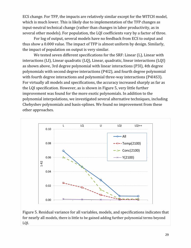
WetestedsevendifferentspecificationsfortheSRF:Linear(L),Linearwithinteractions(LI),Linearquadratic(LQ),Linear,quadratic,linearinteractions(LQI)asshownabove,3rddegreepolynomialwithlinearinteractions(P3I),4thdegreepolynomialswithseconddegreeinteractions(P4I2),andfourthdegreepolynomialwithfourthdegreeinteractionsandpolynomialthree‐wayinteractions(P4I4S3).Forvirtuallyallmodelsandspecifications,theaccuracyincreasedsharplyasfarastheLQIspecification.However,asisshowninFigure5,verylittlefurtherimprovementwasfoundforthemoreexoticpolynomials.Inadditiontothepolynomialinterpolations,weinvestigatedseveralalternativetechniques,includingChebyshevpolynomialsandbasis‐splines.Wefoundnoimprovementfromtheseotherapproaches.
Figure5.Residualvarianceforallvariables,models,andspecificationsindicatesthatfornearlyallmodels,thereislittletobegainedaddingfurtherpolynomialtermsbeyondLQI.
0.00
0.02
0.04
0.06
0.08
0.10L LQ LI LQI LQI++
1‐R2
All
Temp(2100)
Conc(2100)
Y(2100)
30
Insummary,wefoundthatthelinear‐quadratic‐interaction(LQI)specificationofthesurfaceresponsefunctionperformedextremelywellinfittingthedatainourtests.Thereasonisthatthemodels,whilehighlynon‐linearoverall,aregenerallyclosetoquadraticinthethreeuncertainparameters.WearethereforeconfidentthattheyareareliablebasisfortheMonteCarlosimulations.
C.ReliabilityoftheMUPprocedureswithextrapolation
OneissuethatarisesinestimatingthedistributionsofoutcomevariablesistheextenttowhichthecalibrationrunsintrackIadequatelycovertherangeofthepdfsfromtrackII.Forbothpopulationandtheequilibriumtemperaturesensitivity,thecalibrationrunscoveratleast99.9%oftherangeofthepdfs.However,whensettingthecalibrationrangeforTFPbasedonearlierinformalestimates,weunderestimatedthevariabilityofthefinalpdfs.Asaresult,thecalibrationrunsonlyextendasfarasthe83percentileattheupperend,requiringustoextrapolatebeyondtherangeofthecalibrationruns.
Sinceitwasnotpossibletorepeatthecalibrationrunswithanexpandedgrid,wetestedthereliabilityoftheextrapolationandthetwotrackapproachwithtwomodels.WefirstexaminedthereliabilityforTFPwiththebasecaseintheDICEmodel.ThiswasdonebymakingrunswithincrementsofTFPgrowthupto3estimatedstandarddeviations(i.e.,uptoaglobaloutputgrowthrateof6.1%peryearto2100).Theserunscover99.7%ofthedistribution.Wethenestimatedasurfaceresponsefunctionfor2100temperatureoverthesameintervalasforthecalibrationexercisesandextrapolatedoutsidetherange.TheresultsshowedhighreliabilityoftheestimatedSRFfortemperatureincreaseuptoabout2standarddeviationsabovethebaselineTFPgrowthrate.Beyondthat,theSRFtendedtooverestimatethe2100temperature.(SimilarresultswerefoundforCO2concentrationsandthedamage‐outputratiointheDICEmodel.)Thereasonfortheoverestimateisthatcarbonfuelsbecomeexhaustedathighgrowthrates,soraisingthegrowthratefurtherabovethealready‐highratehasarelativelysmalleffectsonemissions,concentrations,2100temperature,andthedamageratio.NotethatthisimpliesthatthefaruppertailofthetemperaturedistributionusingthecorrectedSRFwillshowathinnertailthantheonegeneratedbytheSRFestimatedoverthecalibrationruns.
WealsoperformedamorecomprehensivecomparisonoftheMUPprocedureswithafullMonteCarlousingtheFUNDmodel.Forthis,wetookthepdfsforthethreeuncertainvariablesandranaMonteCarloforthefullFUNDmodelwith1milliondraws.Wethencomparedthemeansandstandarddeviationsofdifferent
31
variablesforthetwoapproaches.WetestedfourdifferentspecificationsoftheSRFstodeterminewhetherthesewouldproducemarkedlydifferentoutcomes.TheresultsindicatedthattheMUPprocedureprovidedreliableestimatesofthemeansandstandarddeviationsofallvariablesthatwetestedexceptFUNDdamages.Exceptingdamages,forthepreferredLQIestimate,theabsoluteaverageerrorofthemeanfortheMUPprocedurerelativetotheFUNDMonteCarlowas0.3%,whiletheabsoluteaverageerrorforthestandarddeviationwas1.2%.Fordamages,theerrorswere7%and44%,respectively.Additionally,thepercentileestimatesfortheMUPprocedure(againexceptfordamages)wereaccurateuptothe90thpercentile.And,aswillbenotedbelow,theestimatesfortheparametersofthetailsofthedistributionswereaccurateforallvariablesexceptdamages.Anoteprovidingfurtherdetailsonthecomparisonsisavailablefromtheauthors.
VII. ResultsoftheMonteCarlosimulations
A. Distributionsformajorvariables
FortheMonteCarlosimulations,wetooktheSRFsforeachparameter/model/year/policyandmade1,000,000drawsfromeachpdfforthethreeuncertainparameters.Wethenexaminedtheresultingdistributions.Thissamplesizewaschosenbecausetheresultswerereliableatthatlevel.Thebootstrapstandarderrorsofthemeansandthestandarddeviationsweregenerallylessthan0.1%ofthemeanorstandarddeviation.Theexceptionwasfordamages,wherethebootstrapstandarderroroftheestimatedstandarddeviationswasabout0.2%ofthevaluefortheFUNDmodel.Wetreateachpdfindependently,butrecognizethattheremaybesomecorrelationbetweenrealizationsofpopulationandGDP.However,explorationsintothisrevealedthatitdidnotsubstantiallyinfluenceourfindings.
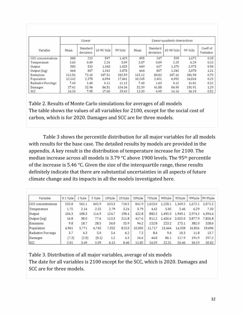
Table2showsstatisticsofthedistributionofthedrawsforeachofthemajoroutcomevariables,withaveragestakenacrossallsixmodels.WealsoshowtheestimatesforthelinearandLQIversionstoillustratethesensitivityoftheresultstotheSRFspecification.Thelastcolumnshowsthecoefficientofvariationforeachvariable.Notethattheseestimatesarewithin‐model(parametricuncertainty)resultsanddonotincludeacross‐modelvariability.Theresultshighlightthatemissions,economicoutput,anddamageshavethehighestcoefficientofvariation,underscoringthattheuncertaintyintheseoutputvariablesisgreaterthanforothervariables,suchasCO2concentrationsandtemperature.Thisistheresultofboththeunderlyingpdfsusedandthemodelsthemselves.
32
Table3showsthepercentiledistributionforallmajorvariablesforallmodelswithresultsforthebasecase.Thedetailedresultsbymodelsareprovidedintheappendix.Akeyresultisthedistributionoftemperatureincreasefor2100.Themedianincreaseacrossallmodelsis3.79°Cabove1900levels.The95thpercentileoftheincreaseis5.46°C.Giventhesizeoftheinterquartilerange,theseresultsdefinitelyindicatethattherearesubstantialuncertaintiesinallaspectsoffutureclimatechangeanditsimpactsinallthemodelsinvestigatedhere.
Table2.ResultsofMonteCarlosimulationsforaveragesofallmodelsThetableshowsthevaluesofallvariablesfor2100,exceptforthesocialcostofcarbon,whichisfor2020.DamagesandSCCareforthreemodels.
Table3.Distributionofallmajorvariables,averageofsixmodelsThedateforallvariablesis2100exceptfortheSCC,whichis2020.DamagesandSCCareforthreemodels.
33
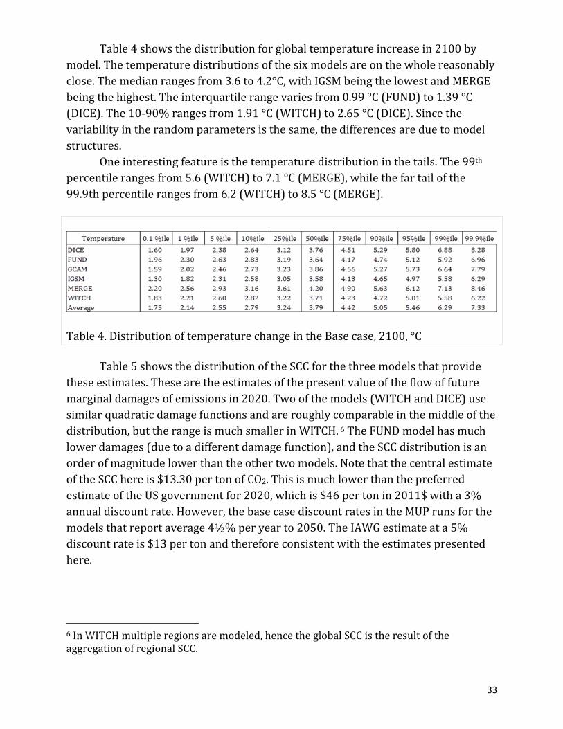
Table4showsthedistributionforglobaltemperatureincreasein2100bymodel.Thetemperaturedistributionsofthesixmodelsareonthewholereasonablyclose.Themedianrangesfrom3.6to4.2°C,withIGSMbeingthelowestandMERGEbeingthehighest.Theinterquartilerangevariesfrom0.99°C(FUND)to1.39°C(DICE).The10‐90%rangesfrom1.91°C(WITCH)to2.65°C(DICE).Sincethevariabilityintherandomparametersisthesame,thedifferencesareduetomodelstructures. Oneinterestingfeatureisthetemperaturedistributioninthetails.The99thpercentilerangesfrom5.6(WITCH)to7.1°C(MERGE),whilethefartailofthe99.9thpercentilerangesfrom6.2(WITCH)to8.5°C(MERGE).
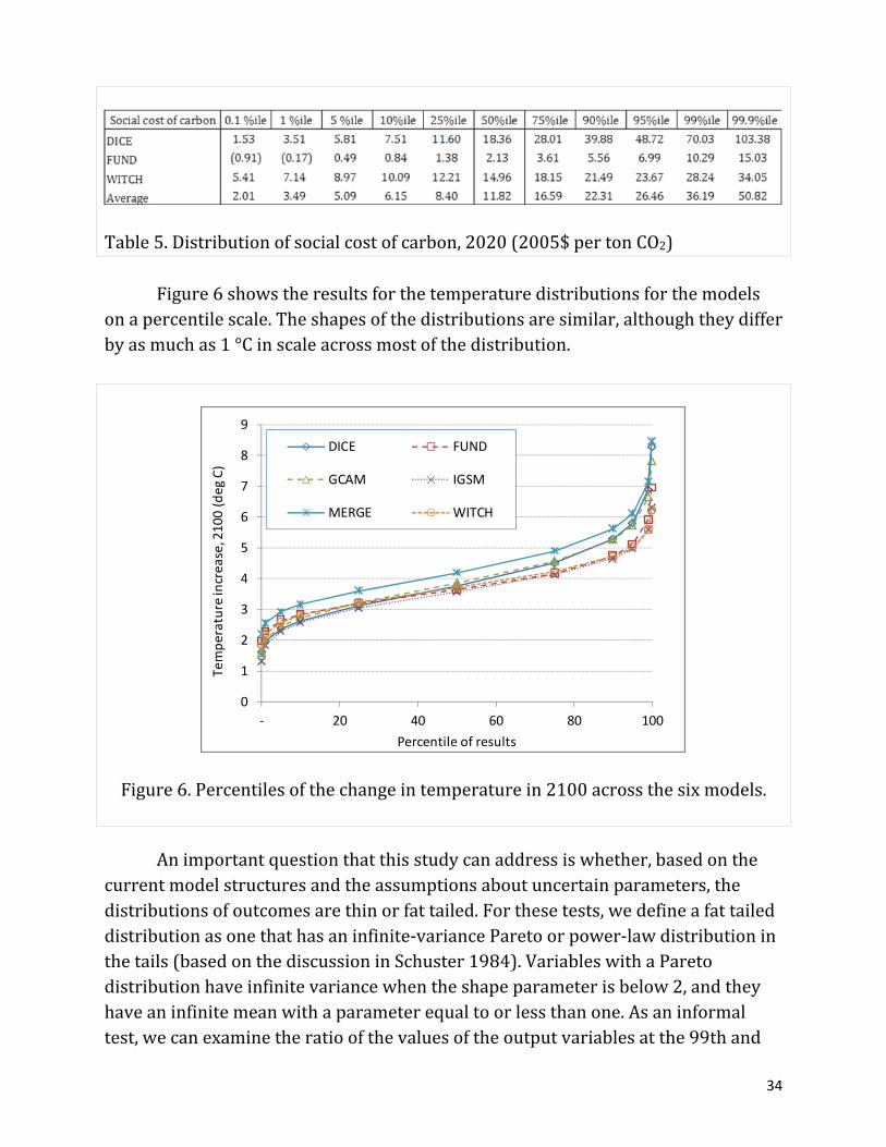
Table5showsthedistributionoftheSCCforthethreemodelsthatprovidetheseestimates.Thesearetheestimatesofthepresentvalueoftheflowoffuturemarginaldamagesofemissionsin2020.Twoofthemodels(WITCHandDICE)usesimilarquadraticdamagefunctionsandareroughlycomparableinthemiddleofthedistribution,buttherangeismuchsmallerinWITCH.6TheFUNDmodelhasmuchlowerdamages(duetoadifferentdamagefunction),andtheSCCdistributionisanorderofmagnitudelowerthantheothertwomodels.NotethatthecentralestimateoftheSCChereis$13.30pertonofCO2.ThisismuchlowerthanthepreferredestimateoftheUSgovernmentfor2020,whichis$46pertonin2011$witha3%annualdiscountrate.However,thebasecasediscountratesintheMUPrunsforthemodelsthatreportaverage4½%peryearto2050.TheIAWGestimateata5%discountrateis$13pertonandthereforeconsistentwiththeestimatespresentedhere.
6InWITCHmultipleregionsaremodeled,hencetheglobalSCCistheresultoftheaggregationofregionalSCC.
Table4.DistributionoftemperaturechangeintheBasecase,2100,°C
34
Figure6showstheresultsforthetemperaturedistributionsforthemodelsonapercentilescale.Theshapesofthedistributionsaresimilar,althoughtheydifferbyasmuchas1°Cinscaleacrossmostofthedistribution.
Animportantquestionthatthisstudycanaddressiswhether,basedonthecurrentmodelstructuresandtheassumptionsaboutuncertainparameters,thedistributionsofoutcomesarethinorfattailed.Forthesetests,wedefineafattaileddistributionasonethathasaninfinite‐varianceParetoorpower‐lawdistributioninthetails(basedonthediscussioninSchuster1984).VariableswithaParetodistributionhaveinfinitevariancewhentheshapeparameterisbelow2,andtheyhaveaninfinitemeanwithaparameterequaltoorlessthanone.Asaninformaltest,wecanexaminetheratioofthevaluesoftheoutputvariablesatthe99thand
Table5.Distributionofsocialcostofcarbon,2020(2005$pertonCO2)
Figure6.Percentilesofthechangeintemperaturein2100acrossthesixmodels.
0
1
2
3
4
5
6
7
8
9
‐ 20 40 60 80 100
Temperature increase, 2100 (deg C)
Percentile of results
DICE FUND
GCAM IGSM
MERGE WITCH
35
99.9thpercentile.Foranormaldistribution,theratiooftheseis1.33.ForParetodistributionswithslopevaluesof2.0,1.8,and1.5,theratiosare3.7,3.9,and5.2.IfweexaminetheMonteCarloestimates,themaximumratiois1.56,whichoccursfordamagesintheDICEandFUNDmodels.Whilethissuggestsatailthatisslightlyfatterthanthenormaldistribution,itfallsfarshortoftheslopeassociatedwithaninfinite‐varianceParetoprocess.
Beforepresentingtheresults,wereiteratetheconcernthatthecalibrationrunsdonotextendfarintothetailsforTFP.ThisimpliesthattheresultsontailsreportedhererelyonextrapolationsoftheSRFoutsidethesamplerange.WecommentbelowonourreplicationofthetailestimateswiththeFUNDmodel,whicharegenerallyaccurate.Wealsoemphasizethattheestimatesofthetailsarederivedfromtheinteractionofthemodelswiththeassumedpdfs.Totheextentthatthemodelsomitdiscontinuitiesorsharpnon‐linearities,orthatourassumedpdfsaretoothin‐tailed,thenwemayunderestimatethethicknessofthetails.
WecanalsouseaformaltestoftheParetoshapeparameter,althoughthisismorecomplicatedbecauseitrequiresassumptionsabouttheminimumoftheParetoregion(statisticaltechniquesarefromRytgaard1990).Examiningthetop10%ofthedamagedistributionfortheDICEmodel(themostskewedofthevariables),wefindthattheparameteroftheParetodistributionabovethe1%righttailisestimatedtobe4.7(+0.047),whichiswellbelowtheinfinite‐variancethresholdof2.TheParetoparameterestimateforthe0.1%tailis7.03(+0.22).Thesetestsrejectthehypothesisthatthedistributionsarefat‐tailedinthesenseofbelongingtoaninfinite‐varianceParetodistribution.Theresultsareduetoboththestructuresofthemodelsandthenatureoftheshocks.Nothinginthemodelspreventsthegenerationoffattailsinthissituation,buttheymaymisscriticalnon‐linearities,sothetestsarenotbyanymeansconclusive.
WeexaminedthevalidityoftheresultsforthetailsusingthefullMonteCarloestimateoftheFUNDmodeldiscussedabove.Forthese,wecomparedtheinformaltests(ratioofthevariablesatthe99.9%iletothe99%ile).TheMUPcalculationswereveryaccurateforallvariablesexceptdamages,whereasfordamagestheMUPcalculationsunderestimatedtheskewness(overestimatedtheParetotail).WealsoexaminedtheParetoparameterinthefullFUNDMonteCarloandfoundthattheestimatewassignificantlyabovethethresholdofaninfinitevarianceprocess.
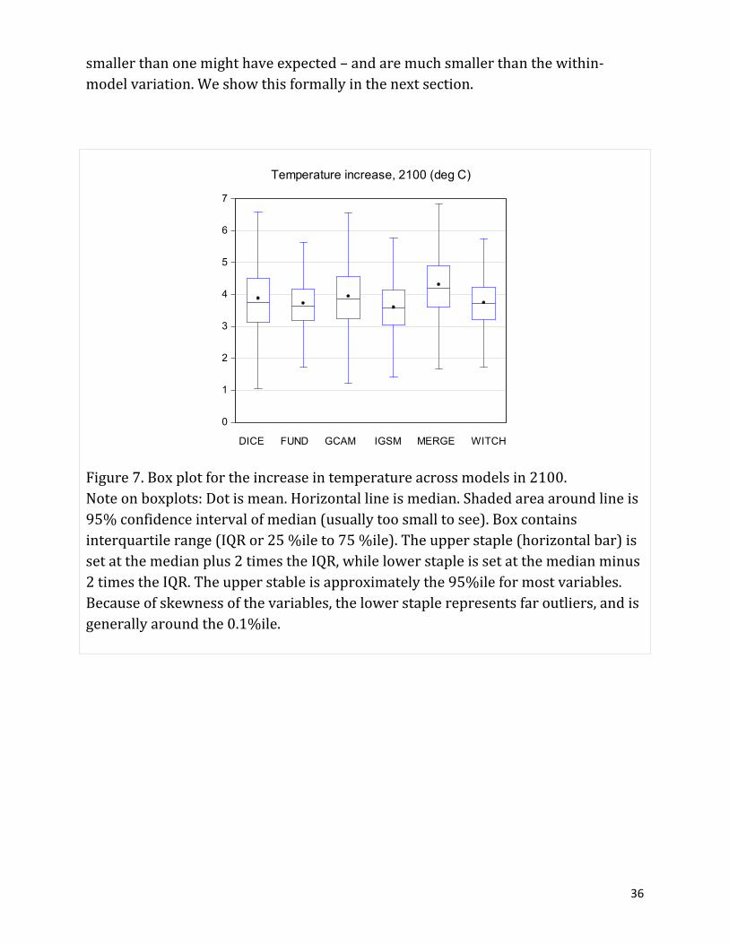
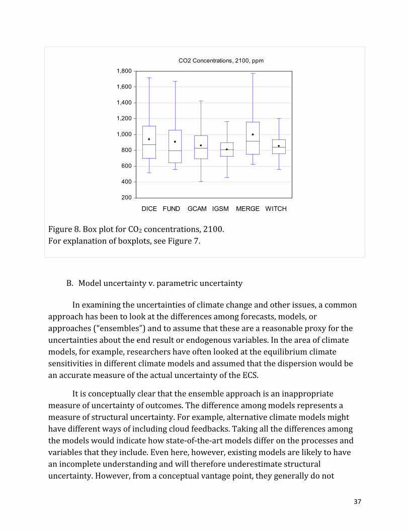
Theresultscanalsobeseeninboxplots.Figure7showstheboxplotfortemperatureincreaseto2100.Figure8showstheboxplotfortheCO2concentrationsfor2100.Bothoftheseunderscorethatwhiletherearedifferencesbetweenthemodelsinthewaythattheyarerunforthisstudy,theyareperhaps
36
smallerthanonemighthaveexpected–andaremuchsmallerthanthewithin‐modelvariation.Weshowthisformallyinthenextsection.
0
1
2
3
4
5
6
7
DICE FUND GCAM IGSM MERGE WITCH
Temperature increase, 2100 (deg C)
Figure7.Boxplotfortheincreaseintemperatureacrossmodelsin2100.Noteonboxplots:Dotismean.Horizontallineismedian.Shadedareaaroundlineis95%confidenceintervalofmedian(usuallytoosmalltosee).Boxcontainsinterquartilerange(IQRor25%ileto75%ile).Theupperstaple(horizontalbar)issetatthemedianplus2timestheIQR,whilelowerstapleissetatthemedianminus2timestheIQR.Theupperstableisapproximatelythe95%ileformostvariables.Becauseofskewnessofthevariables,thelowerstaplerepresentsfaroutliers,andisgenerallyaroundthe0.1%ile.
37
B. Modeluncertaintyv.parametricuncertainty
Inexaminingtheuncertaintiesofclimatechangeandotherissues,acommonapproachhasbeentolookatthedifferencesamongforecasts,models,orapproaches(“ensembles”)andtoassumethattheseareareasonableproxyfortheuncertaintiesabouttheendresultorendogenousvariables.Intheareaofclimatemodels,forexample,researchershaveoftenlookedattheequilibriumclimatesensitivitiesindifferentclimatemodelsandassumedthatthedispersionwouldbeanaccuratemeasureoftheactualuncertaintyoftheECS.
Itisconceptuallyclearthattheensembleapproachisaninappropriatemeasureofuncertaintyofoutcomes.Thedifferenceamongmodelsrepresentsameasureofstructuraluncertainty.Forexample,alternativeclimatemodelsmighthavedifferentwaysofincludingcloudfeedbacks.Takingallthedifferencesamongthemodelswouldindicatehowstate‐of‐the‐artmodelsdifferontheprocessesandvariablesthattheyinclude.Evenhere,however,existingmodelsarelikelytohaveanincompleteunderstandingandwillthereforeunderestimatestructuraluncertainty.However,fromaconceptualvantagepoint,theygenerallydonot
200
400
600
800
1,000
1,200
1,400
1,600
1,800
DICE FUND GCAM IGSM MERGE WITCH
CO2 Concentrations, 2100, ppm
Figure8.BoxplotforCO2concentrations,2100.Forexplanationofboxplots,seeFigure7.
38
explicitlymodelandconsiderparametricuncertainty.InIAMs,tocomeclosertohome,differencesinmodelsreflectdifferencesinassumptionsaboutgrowthrates,productionfunctions,energysystems,andthelike.Butfewmodelsexplicitlyincludeparametricuncertaintyaboutthesevariables.Differencesinpopulationgrowth,forexample,areverysmallrelativetomeasuresofuncertaintybasedonstatisticaltechniquesbecausemanymodelsusethesameestimatesoflong‐runpopulationtrends.
WecanusetheresultsoftheMonteCarlosimulationstoestimatetherelativeimportanceofparametricuncertaintyandmodeluncertainty.WecanwritetheresultsoftheMonteCarlosimulationsschematicallyasfollows.Assumethatthe
modeloutcomeforvariableiandmodelmis miY andthattheuncertainparameters
are and i ju u :
3 3
,1 1 1
jm m m m
i i i i i j i ji j i
Y u u u
Foragivendistributionofeachoftheuncertainparameters,thevarianceof iY
includingmodelvariationis:
3 32 2 2 2 2 2 2
,1 1 1
( ) ( ) ( ) ( ) ( ) ( ) ( )j
m mi i i i i j i j
i j i
Y u u u
Thefirsttermontherighthandsideisthevarianceduetomodeldifferences(orstructuraluncertainty),whilethesecondandthirdtermsarethevarianceduetoparameteruncertainty.Forthispurpose,weincludetheinteractionofthemodel
coefficients ,( and )m mi i j andtheparameteruncertainties 2[ ( )]iu asparametric
uncertaintybecausetheywouldnotbeincludedinensembleuncertainty.Theothertermsvanishbecauseweassumethattheparametricuncertaintiesareindependent.Whiledependencewilladdfurthertermsontheright‐handsideoftheequationforthevariance,itwillnotaffectthefractionduetostructuraldifferencesduetothefirstterm.
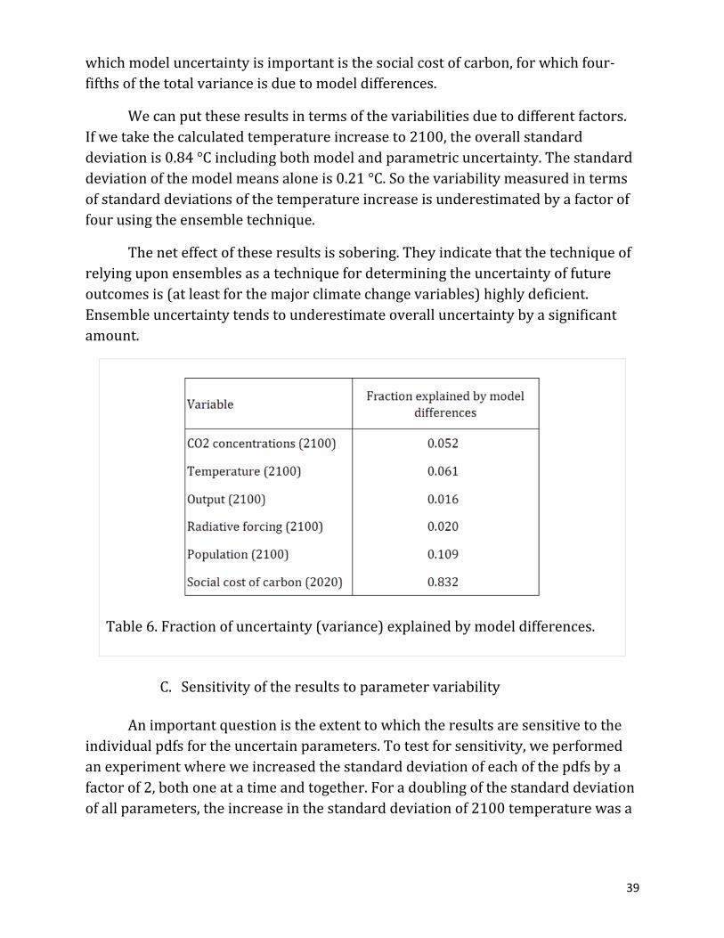
Wecaneasilyestimatethetotaluncertaintyandthestructuraluncertaintyfordifferentvariables.TheresultsareshowninTable6.Formostvariables,virtuallyallthevarianceisexplainedbyparametricuncertainty.Forexample,94%ofthevarianceofthe2100temperatureincreaseinallthemodelsisexplainedbyparametricuncertainty,andonly6%isexplainedbydifferencesinmodelmeans.ThisfactiseasilyseenintheboxchartsinFigures7and8.Theonlyvariablefor
39
whichmodeluncertaintyisimportantisthesocialcostofcarbon,forwhichfour‐fifthsofthetotalvarianceisduetomodeldifferences.
Wecanputtheseresultsintermsofthevariabilitiesduetodifferentfactors.Ifwetakethecalculatedtemperatureincreaseto2100,theoverallstandarddeviationis0.84°Cincludingbothmodelandparametricuncertainty.Thestandarddeviationofthemodelmeansaloneis0.21°C.Sothevariabilitymeasuredintermsofstandarddeviationsofthetemperatureincreaseisunderestimatedbyafactoroffourusingtheensembletechnique.
Theneteffectoftheseresultsissobering.Theyindicatethatthetechniqueofrelyinguponensemblesasatechniquefordeterminingtheuncertaintyoffutureoutcomesis(atleastforthemajorclimatechangevariables)highlydeficient.Ensembleuncertaintytendstounderestimateoveralluncertaintybyasignificantamount.
C. Sensitivityoftheresultstoparametervariability
Animportantquestionistheextenttowhichtheresultsaresensitivetotheindividualpdfsfortheuncertainparameters.Totestforsensitivity,weperformedanexperimentwhereweincreasedthestandarddeviationofeachofthepdfsbyafactorof2,bothoneatatimeandtogether.Foradoublingofthestandarddeviationofallparameters,theincreaseinthestandarddeviationof2100temperaturewasa
Table6.Fractionofuncertainty(variance)explainedbymodeldifferences.
40
factorof1.83forallmodelstogether.Webelievethatthisislessthantwobecausetheshort‐runtemperatureimpactisnotproportionaltotheECS.
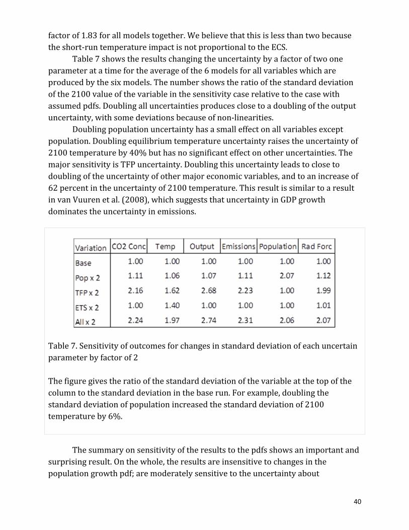
Table7showstheresultschangingtheuncertaintybyafactoroftwooneparameteratatimefortheaverageofthe6modelsforallvariableswhichareproducedbythesixmodels.Thenumbershowstheratioofthestandarddeviationofthe2100valueofthevariableinthesensitivitycaserelativetothecasewithassumedpdfs.Doublingalluncertaintiesproducesclosetoadoublingoftheoutputuncertainty,withsomedeviationsbecauseofnon‐linearities.
Doublingpopulationuncertaintyhasasmalleffectonallvariablesexceptpopulation.Doublingequilibriumtemperatureuncertaintyraisestheuncertaintyof2100temperatureby40%buthasnosignificanteffectonotheruncertainties.ThemajorsensitivityisTFPuncertainty.Doublingthisuncertaintyleadstoclosetodoublingoftheuncertaintyofothermajoreconomicvariables,andtoanincreaseof62percentintheuncertaintyof2100temperature.ThisresultissimilartoaresultinvanVuurenetal.(2008),whichsuggeststhatuncertaintyinGDPgrowthdominatestheuncertaintyinemissions.
Thesummaryonsensitivityoftheresultstothepdfsshowsanimportantandsurprisingresult.Onthewhole,theresultsareinsensitivetochangesinthepopulationgrowthpdf;aremoderatelysensitivetotheuncertaintyabout
Table7.Sensitivityofoutcomesforchangesinstandarddeviationofeachuncertainparameterbyfactorof2Thefiguregivestheratioofthestandarddeviationofthevariableatthetopofthecolumntothestandarddeviationinthebaserun.Forexample,doublingthestandarddeviationofpopulationincreasedthestandarddeviationof2100temperatureby6%.
41
equilibriumtemperaturesensitivityontemperature(aswellastodamagesandthesocialcostofcarbon,notshown);andareextremelysensitivetotheuncertaintyabouttherateofgrowthofproductivity.Whilelong‐runproductivitygrowthhasthegreatestimpactonuncertainty,itisalsotheleastcarefullystudiedofanyoftheparameterswehaveexamined.Thisresultsuggeststhatmuchgreaterattentionshouldbegiventodevelopingreliableestimatesofthetrendanduncertaintiesaboutlong‐runproductivity.
VIII. Conclusions
Thisstudyisthefirstmulti‐modelanalysisofparametricuncertaintyineconomicclimate‐changemodeling.Theapproachisbasedonestimatingclassicstatisticalforecastuncertainty.Thecentralmethodologyconsistsoftwotracks.TrackIinvolvesdoingasetofmodelcalibrationrunsforthesixmodelsandthreeuncertainparametersandestimatingasurfaceresponsefunctionfortheresultsofthoseruns.TrackIIinvolvesdevelopingpdfsforkeyuncertainparameters.ThetwotracksarebroughttogetherthroughasetofMonteCarlosimulationstoestimatetheoutputdistributionsofmultipleoutputvariablesthatareimportantforclimatechangeandclimate‐changepolicy.Thisapproachisreplicableandtransparent,andovercomesseveralobstaclesforexamininguncertaintyinclimatechange.
Herearethekeyresults.First,thecentralprojectionsoftheintegratedassessmentmodels(IAMs)areremarkablysimilaratthemodeler’sbaselineparameters.Thisresultisprobablyduetothefactthatmodelshavebeenusedinmodelcomparisonsandmayhavebeenrevisedtoyieldsimilarbaselineresults.However,theprojectionsdivergesharplywhenalternativeassumptionsaboutthekeyuncertainparametersareused,especiallyathighlevelsofpopulationgrowth,productivitygrowth,andequilibriumclimatesensitivity.
Second,despitethesedifferencesacrossmodelsforalternativeparameters,thedistributionsofthekeyoutputvariablesareremarkablysimilaracrossmodelswithdifferentstructuresandlevelsofcomplexity.Totakeyear2100temperatureasanexample,thequantilesofthedistributionsofthemodelsdifferbylessthan½°Cfortheentiredistributionuptothe95thpercentile.
Third,wefindthattheclimate‐relatedvariablesarecharacterizedbylowuncertaintyrelativetothoserelatingtomosteconomicvariables.Forthiscomparison,welookatthecoefficientofvariation(CV)oftheMonteCarlosimulations.AsshowninTable2,CO2concentrations,radiativeforcings,andtemperature(allfor2100)haverelativelylowCV.OutputanddamageshaverelativelyhighCV.Asexamples,themodel‐averagecoefficientofvariationforcarbondioxideconcentrationsin2100is0.28,whilethecoefficientofvariationfor
42
climate‐changedamagesis1.29.ThesocialcostofcarbonhasanintermediateCVwithinmodels,butwhenmodelvariationisincludedtheCVisclosetothatofoutputanddamages.Theseresultshighlighttheimportanceoffurtherresearchoneconomicvariablesanddamagefunctionsforreducinguncertaintyandimprovingpolicymaking(e.g.,seePizeretal.2014andDrouetetal.2015).
Fourth,wefindmuchgreaterparametricuncertaintythanstructural(acrossmodel)uncertaintyforalloutputvariablesexceptthesocialcostofcarbon.Forexample,inexaminingtheuncertaintyin2100temperatureincrease,thedifferenceofmodelmeans(ortheensembleuncertainty)isapproximatelyone‐quarterofthetotaluncertainty,withtherestdrivenbyparametricuncertainty.Whilelookingacrosssixmodelsbynomeansspansthespaceofmethods,thesixmodelsexaminedherearerepresentativeofthedifferencesinsize,structure,andcomplexityofIAMs.Thisresultisimportantbecauseofthewidespreaduseofensembleuncertaintyasaproxyforoveralluncertaintyandhighlightstheneedforare‐orientationofresearchtowardsexaminingparametricuncertaintyacrossmodels.
Afifthinterestingfindingofthisanalysisisthelackofevidenceinsupportoffattailsinthedistributionsofemissions,globalmeansurfacetemperature,ordamages.Populationgrowth,totalfactorproductivitygrowth,andclimatesensitivityareverylikelytobethreeofthekeyuncertainparametersinclimatechange.Yet,basedonbothinformalandformaltests,themodelsascurrentlyconstructedfindthatthetailsarerelativelythin.Thedeclineinprobabilitiesassociatedwithachangeinanyofthevariablesismuchlargerthanwouldbeassociatedwithaninfinite‐varianceParetoprocess.Asdiscussedabove,weemphasizethatthesefindingsshouldbeinterpretedinthecontextofthecurrentgroupofmodelsandtheassumedpdfs.Theresultsdonotruleoutfattails,buttheydoprovideempiricalevidenceagainstfattailsinoutcomesinvestigatedinthisstudyforthecurrentsetofmodelsandthedistributionsofthethreeuncertainvariablesconsideredhere.Theseresultstendtosupporttheuseofexpectedbenefit‐costanalysisforclimatechangepolicy,incontrasttosuggestionsbysomeauthorsthatneglectoffattaileventsmayvitiatestandardanalyses(Weitzman2009).
Sixth,wefindthatwithinawiderangeofuncertainty,changesindispersionoftwooftheuncertainparameterstakensinglyhavearelativelysmalleffectontheuncertaintyoftheoutputvariables,thesebeingpopulationgrowthandequilibriumtemperaturesensitivity.However,uncertaintyaboutproductivitygrowthhasamajorimpactontheuncertaintyofallthemajoroutputvariables.Thereasonforthisisthattheuncertaintyofproductivitygrowthfromtheexpertsurveycompoundsgreatlyoverthe21stcenturyandinducesanextremelylargeuncertainty
43
aboutoutput,emissions,concentrations,temperaturechange,anddamagesbytheendofthecentury. Asinanystudy,thisanalysisisintentionallysharplyfocused.Byanalyzingparametricuncertaintyinthreekeyparameters,wedonotclaimtobecapturingalluncertaintiesinclimatechange.Aswedescribeabove,therearemanyuncertaintiesthatcannotbecapturedusingthestatisticalframeworkdevelopedhere.ButbyprovidingdetailedestimatesofuncertaintyacrossarangeofIAMsthatarecurrentlybeingusedinthepolicyprocess,webelievethatwehavesignificantlyimprovedtheunderstandingofuncertaintyinclimatechange.Moreover,ournewtwo‐trackmethodologyiswell‐suitedforexpansiontoadditionalparametersandmodels,andcanbereadilyusedtoexploreadditionalconcerns,suchastheinteractionbetweencarbonpoliciesanduncertainty.
44
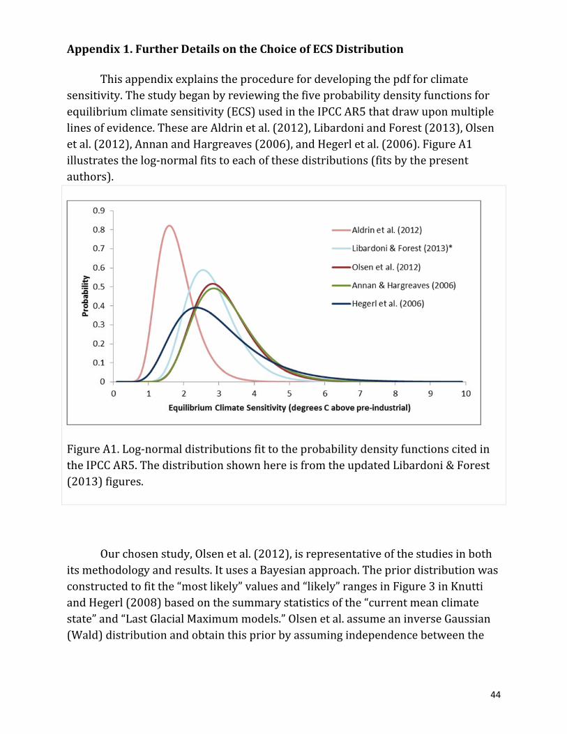
Appendix1.FurtherDetailsontheChoiceofECSDistribution
Thisappendixexplainstheprocedurefordevelopingthepdfforclimatesensitivity.Thestudybeganbyreviewingthefiveprobabilitydensityfunctionsforequilibriumclimatesensitivity(ECS)usedintheIPCCAR5thatdrawuponmultiplelinesofevidence.TheseareAldrinetal.(2012),LibardoniandForest(2013),Olsenetal.(2012),AnnanandHargreaves(2006),andHegerletal.(2006).FigureA1illustratesthelog‐normalfitstoeachofthesedistributions(fitsbythepresentauthors).
Ourchosenstudy,Olsenetal.(2012),isrepresentativeofthestudiesinbothitsmethodologyandresults.ItusesaBayesianapproach.Thepriordistributionwasconstructedtofitthe“mostlikely”valuesand“likely”rangesinFigure3inKnuttiandHegerl(2008)basedonthesummarystatisticsofthe“currentmeanclimatestate”and“LastGlacialMaximummodels.”Olsenetal.assumeaninverseGaussian(Wald)distributionandobtainthispriorbyassumingindependencebetweenthe
FigureA1.Log‐normaldistributionsfittotheprobabilitydensityfunctionscitedintheIPCCAR5.ThedistributionshownhereisfromtheupdatedLibardoni&Forest(2013)figures.
45
currentmeanclimatestateandthelastglacialmaximummodels,andthencomputingthemixturedistribution.
TheposteriordistributionisthencalculatedbyusingaMarkovChainMonteCarlosimulationtoupdatethepriorwithalikelihoodfunction.Thelikelihoodisbasedonseveraldifferenttracers,suchasglobalaverageatmosphericsurface/oceansurfacetemperaturesandglobaltotalheatcontent.ThesetracerscomefromtheUniversityofVictoriaESCMclimatemodel,whichconsistsofathree‐dimensionaloceangeneralcirculationmodelcoupledwithathermodynamic/dynamicsea‐icemodel.Theauthorsassumeindependence,sothatthelikelihoodofbothobservationsisequaltotheproductofthelikelihoods.
Theparametersofthelog‐normaldistributionfittoOlsenetal.areμ=1.10704andσ=0.264.Themajorsummarystatisticsofthereferencedistributioninthestudyarethefollowing:mean=3.13,median=3.03,standarddeviation=0.843,skewness=0.824,andkurtosis=4.23.InimplementingtheMonteCarloforeachmodel,weretainedthemeanECSforthatmodel.Wethenimposedalog‐normaldistributionthatretainedthearithmeticstandarddeviationoftheECS(i.e.,astandarddeviationof0.843)basedontheOlsenetal.(2012)distribution.
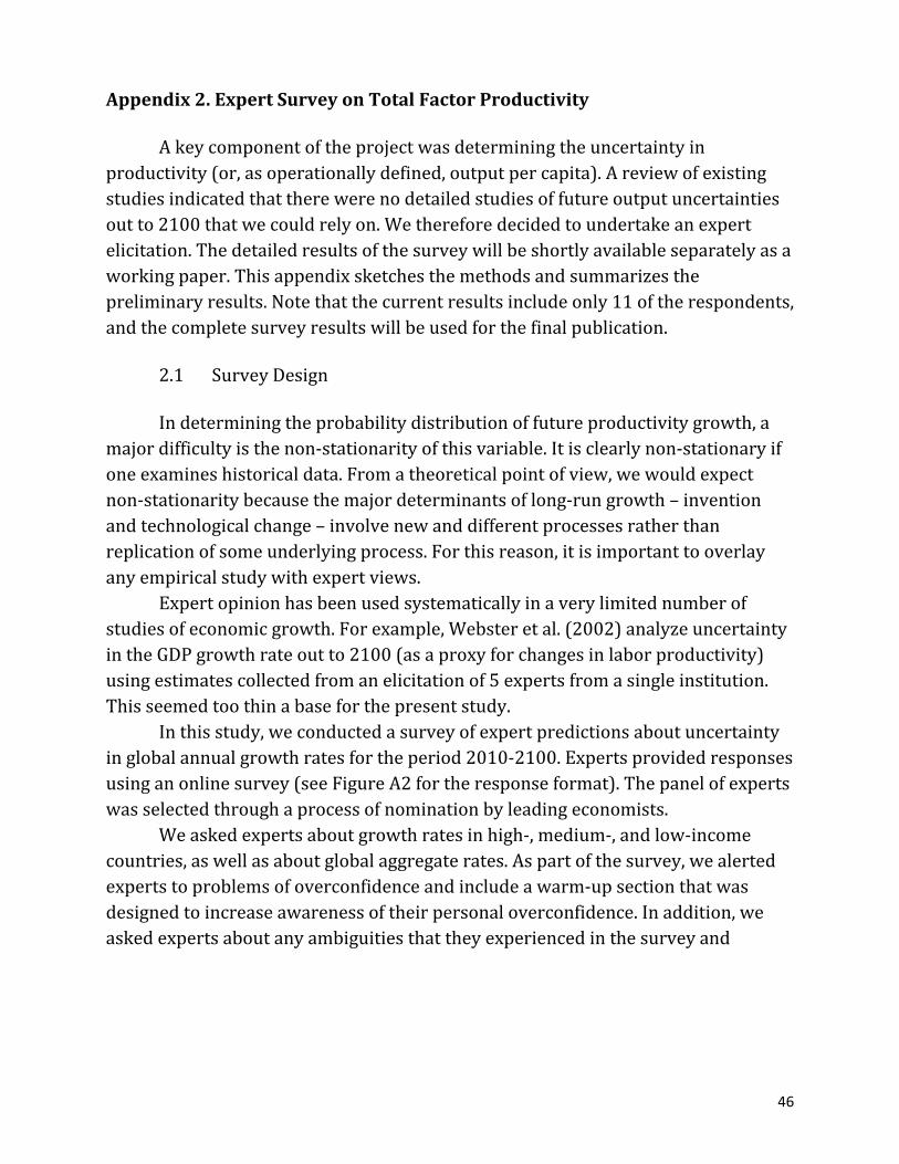
46
Appendix2.ExpertSurveyonTotalFactorProductivity
Akeycomponentoftheprojectwasdeterminingtheuncertaintyinproductivity(or,asoperationallydefined,outputpercapita).Areviewofexistingstudiesindicatedthattherewerenodetailedstudiesoffutureoutputuncertaintiesoutto2100thatwecouldrelyon.Wethereforedecidedtoundertakeanexpertelicitation.Thedetailedresultsofthesurveywillbeshortlyavailableseparatelyasaworkingpaper.Thisappendixsketchesthemethodsandsummarizesthepreliminaryresults.Notethatthecurrentresultsincludeonly11oftherespondents,andthecompletesurveyresultswillbeusedforthefinalpublication.
2.1 SurveyDesign
Indeterminingtheprobabilitydistributionoffutureproductivitygrowth,amajordifficultyisthenon‐stationarityofthisvariable.Itisclearlynon‐stationaryifoneexamineshistoricaldata.Fromatheoreticalpointofview,wewouldexpectnon‐stationaritybecausethemajordeterminantsoflong‐rungrowth–inventionandtechnologicalchange–involvenewanddifferentprocessesratherthanreplicationofsomeunderlyingprocess.Forthisreason,itisimportanttooverlayanyempiricalstudywithexpertviews.
Expertopinionhasbeenusedsystematicallyinaverylimitednumberofstudiesofeconomicgrowth.Forexample,Websteretal.(2002)analyzeuncertaintyintheGDPgrowthrateoutto2100(asaproxyforchangesinlaborproductivity)usingestimatescollectedfromanelicitationof5expertsfromasingleinstitution.Thisseemedtoothinabaseforthepresentstudy.
Inthisstudy,weconductedasurveyofexpertpredictionsaboutuncertaintyinglobalannualgrowthratesfortheperiod2010‐2100.Expertsprovidedresponsesusinganonlinesurvey(seeFigureA2fortheresponseformat).Thepanelofexpertswasselectedthroughaprocessofnominationbyleadingeconomists.
Weaskedexpertsaboutgrowthratesinhigh‐,medium‐,andlow‐incomecountries,aswellasaboutglobalaggregaterates.Aspartofthesurvey,wealertedexpertstoproblemsofoverconfidenceandincludeawarm‐upsectionthatwasdesignedtoincreaseawarenessoftheirpersonaloverconfidence.Inaddition,weaskedexpertsaboutanyambiguitiesthattheyexperiencedinthesurveyand
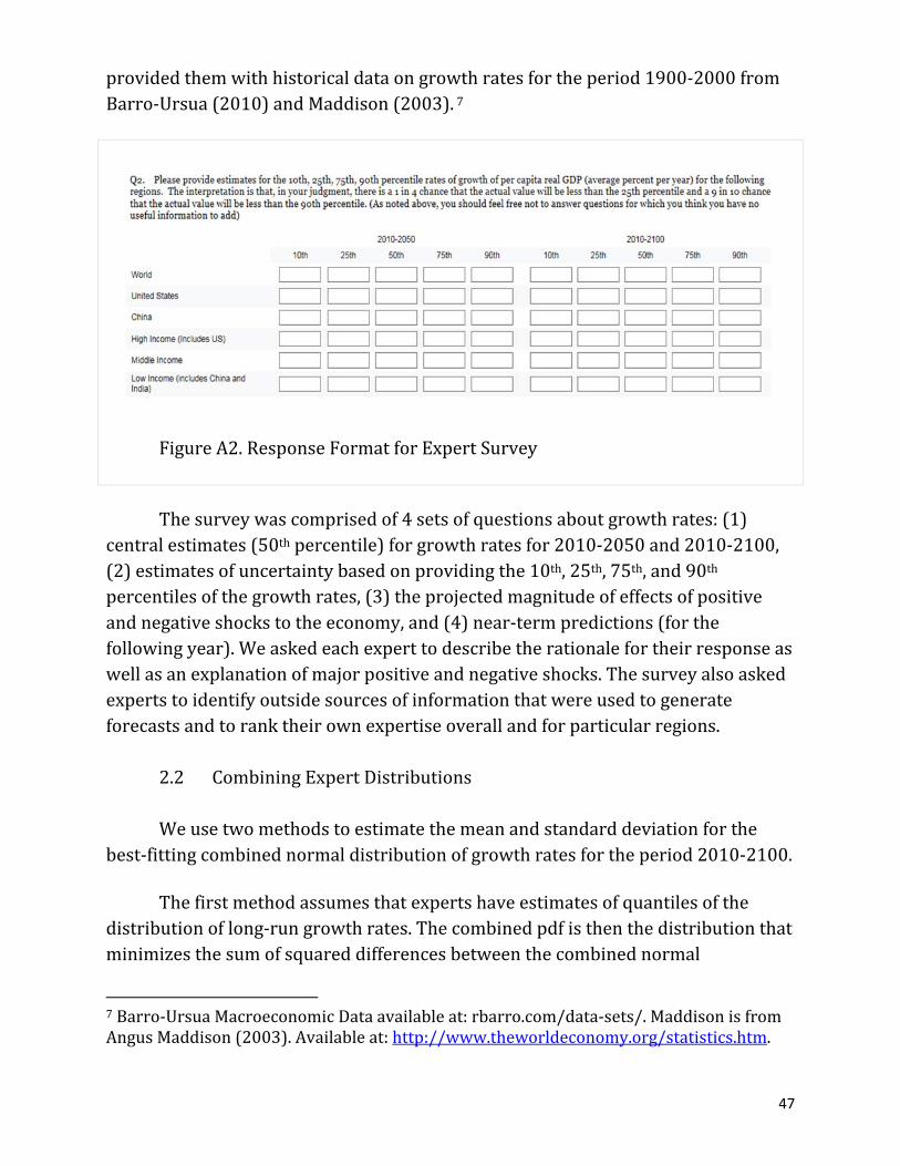
47
providedthemwithhistoricaldataongrowthratesfortheperiod1900‐2000fromBarro‐Ursua(2010)andMaddison(2003).7
Thesurveywascomprisedof4setsofquestionsaboutgrowthrates:(1)centralestimates(50thpercentile)forgrowthratesfor2010‐2050and2010‐2100,(2)estimatesofuncertaintybasedonprovidingthe10th,25th,75th,and90thpercentilesofthegrowthrates,(3)theprojectedmagnitudeofeffectsofpositiveandnegativeshockstotheeconomy,and(4)near‐termpredictions(forthefollowingyear).Weaskedeachexperttodescribetherationalefortheirresponseaswellasanexplanationofmajorpositiveandnegativeshocks.Thesurveyalsoaskedexpertstoidentifyoutsidesourcesofinformationthatwereusedtogenerateforecastsandtoranktheirownexpertiseoverallandforparticularregions.
2.2 CombiningExpertDistributions
Weusetwomethodstoestimatethemeanandstandarddeviationforthe
best‐fittingcombinednormaldistributionofgrowthratesfortheperiod2010‐2100.
Thefirstmethodassumesthatexpertshaveestimatesofquantilesofthedistributionoflong‐rungrowthrates.Thecombinedpdfisthenthedistributionthatminimizesthesumofsquareddifferencesbetweenthecombinednormal
7Barro‐UrsuaMacroeconomicDataavailableat:rbarro.com/data‐sets/.MaddisonisfromAngusMaddison(2003).Availableat:http://www.theworldeconomy.org/statistics.htm.
FigureA2.ResponseFormatforExpertSurvey
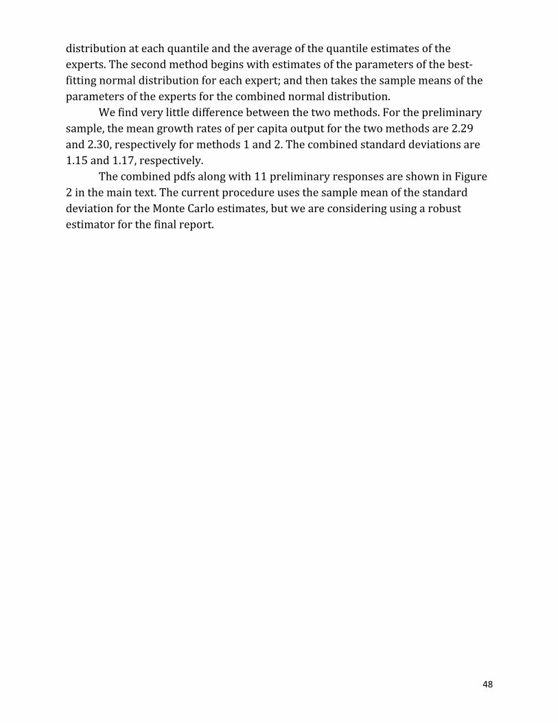
48
distributionateachquantileandtheaverageofthequantileestimatesoftheexperts.Thesecondmethodbeginswithestimatesoftheparametersofthebest‐fittingnormaldistributionforeachexpert;andthentakesthesamplemeansoftheparametersoftheexpertsforthecombinednormaldistribution.
Wefindverylittledifferencebetweenthetwomethods.Forthepreliminarysample,themeangrowthratesofpercapitaoutputforthetwomethodsare2.29and2.30,respectivelyformethods1and2.Thecombinedstandarddeviationsare1.15and1.17,respectively.
Thecombinedpdfsalongwith11preliminaryresponsesareshowninFigure2inthemaintext.ThecurrentprocedureusesthesamplemeanofthestandarddeviationfortheMonteCarloestimates,butweareconsideringusingarobustestimatorforthefinalreport.
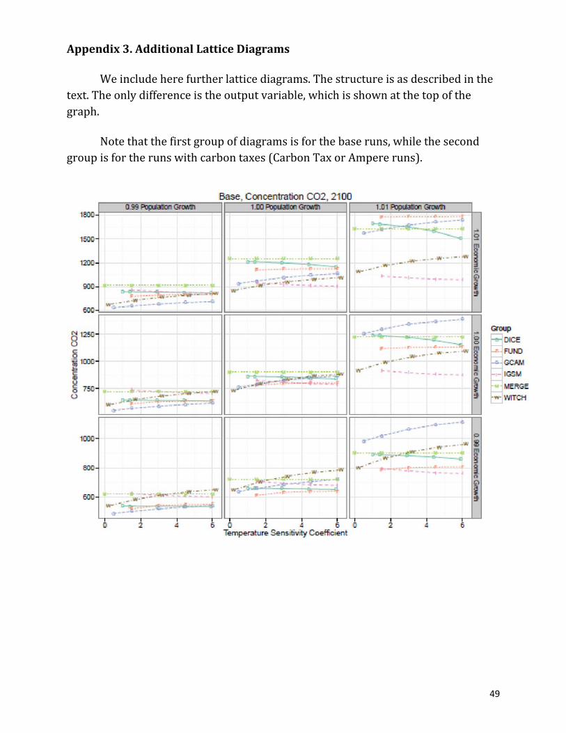
49
Appendix3.AdditionalLatticeDiagrams
Weincludeherefurtherlatticediagrams.Thestructureisasdescribedinthetext.Theonlydifferenceistheoutputvariable,whichisshownatthetopofthegraph.
Notethatthefirstgroupofdiagramsisforthebaseruns,whilethesecondgroupisfortherunswithcarbontaxes(CarbonTaxorAmpereruns).
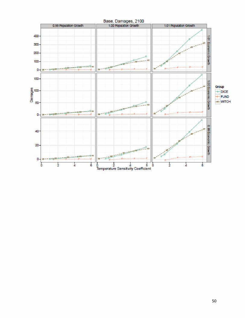
50
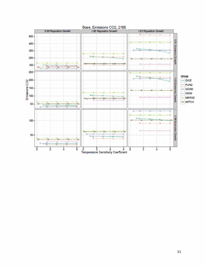
51
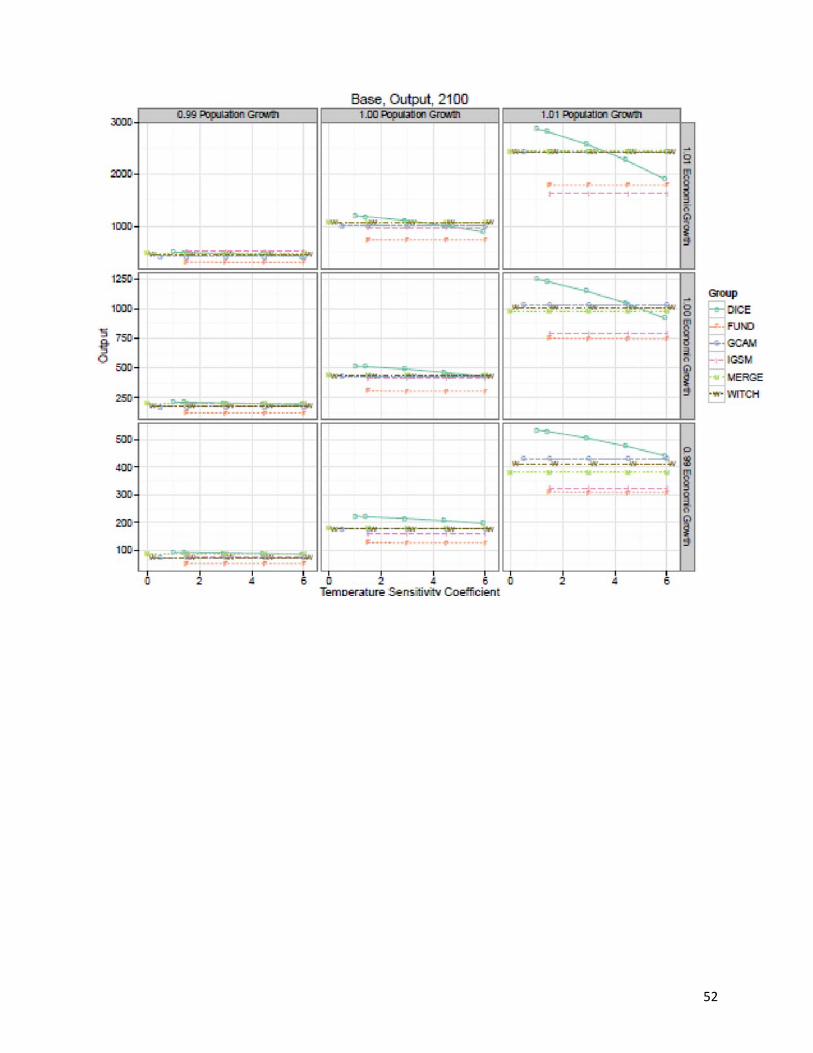
52
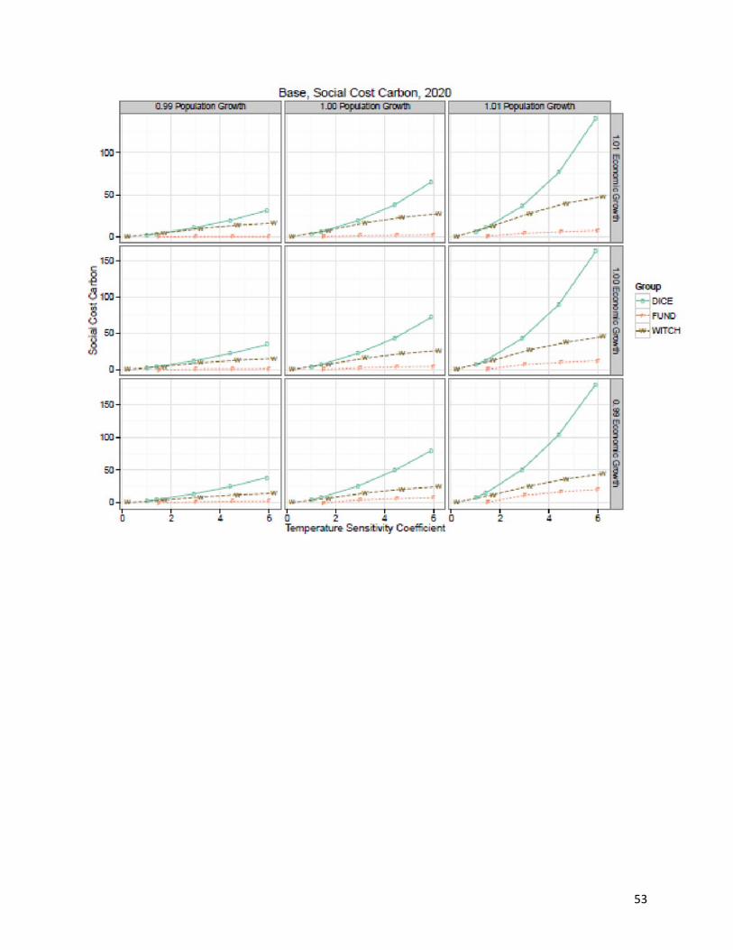
53
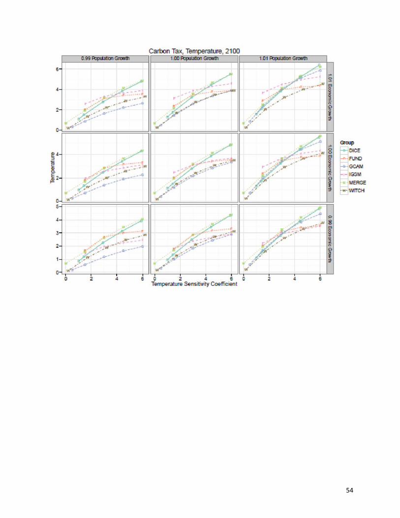
54
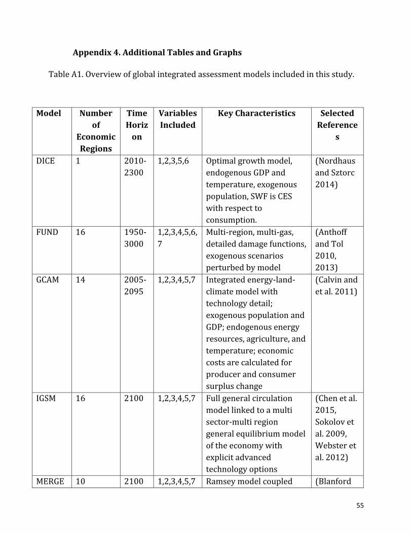
55
Appendix4.AdditionalTablesandGraphs
TableA1.Overviewofglobalintegratedassessmentmodelsincludedinthisstudy.
Model Numberof
EconomicRegions
TimeHorizon
VariablesIncluded
KeyCharacteristics SelectedReference
s
DICE 1 2010‐2300
1,2,3,5,6 Optimalgrowthmodel,endogenousGDPandtemperature,exogenouspopulation,SWFisCESwithrespecttoconsumption.
(NordhausandSztorc2014)
FUND 16 1950‐3000
1,2,3,4,5,6,7
Multi‐region,multi‐gas,detaileddamagefunctions,exogenousscenariosperturbedbymodel
(AnthoffandTol2010,2013)
GCAM 14 2005‐2095
1,2,3,4,5,7 Integratedenergy‐land‐climatemodelwithtechnologydetail;exogenouspopulationandGDP;endogenousenergyresources,agriculture,andtemperature;economiccostsarecalculatedforproducerandconsumersurpluschange
(Calvinandetal.2011)
IGSM 16
2100 1,2,3,4,5,7 Fullgeneralcirculationmodellinkedtoamultisector‐multiregiongeneralequilibriummodeloftheeconomywithexplicitadvancedtechnologyoptions
(Chenetal.2015,Sokolovetal.2009,Websteretal.2012)
MERGE 10 2100 1,2,3,4,5,7 Ramseymodelcoupled (Blanford
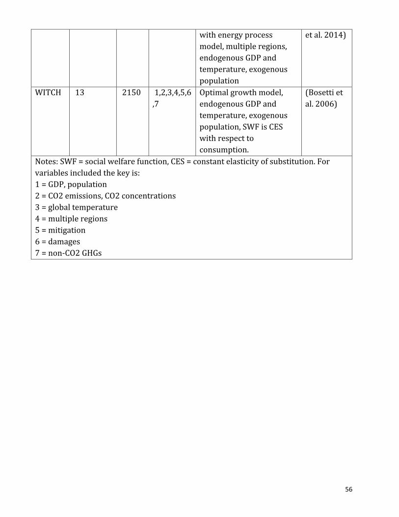
56
withenergyprocessmodel,multipleregions,endogenousGDPandtemperature,exogenouspopulation
etal.2014)
WITCH 13 2150 1,2,3,4,5,6,7
Optimalgrowthmodel,endogenousGDPandtemperature,exogenouspopulation,SWFisCESwithrespecttoconsumption.
(Bosettietal.2006)
Notes:SWF=socialwelfarefunction,CES=constantelasticityofsubstitution.Forvariablesincludedthekeyis:1=GDP,population2=CO2emissions,CO2concentrations3=globaltemperature4=multipleregions5=mitigation6=damages7=non‐CO2GHGs
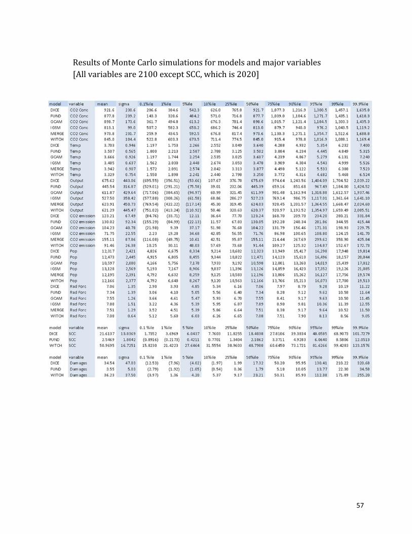
57
ResultsofMonteCarlosimulationsformodelsandmajorvariables[Allvariablesare2100exceptSCC,whichis2020]
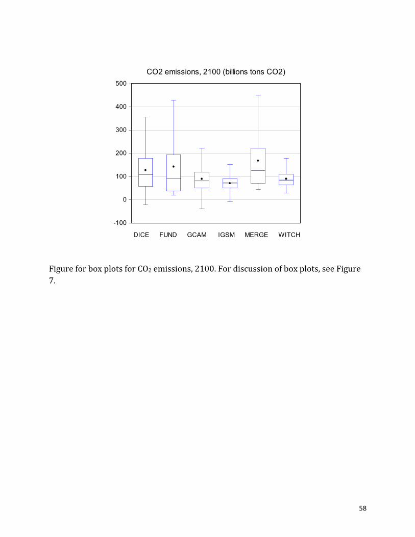
58
FigureforboxplotsforCO2emissions,2100.Fordiscussionofboxplots,seeFigure7.
-100
0
100
200
300
400
500
DICE FUND GCAM IGSM MERGE WITCH
CO2 emissions, 2100 (billions tons CO2)
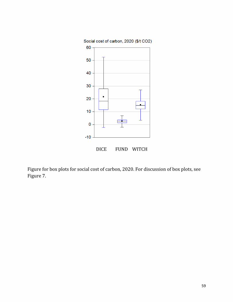
59
DICEFUNDWITCH
Figureforboxplotsforsocialcostofcarbon,2020.Fordiscussionofboxplots,seeFigure7.
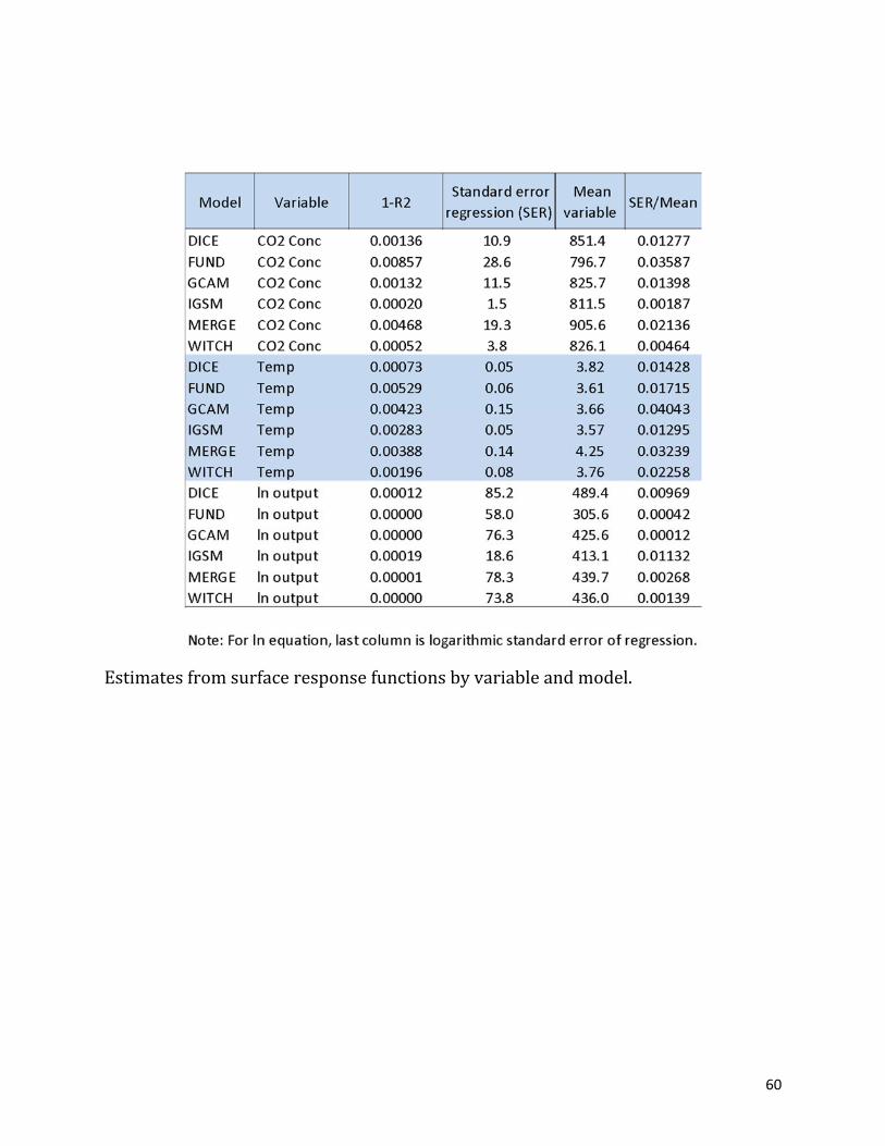
60
Estimatesfromsurfaceresponsefunctionsbyvariableandmodel.
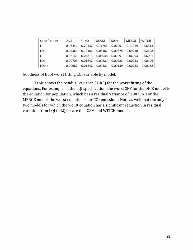
61
GoodnessoffitofworstfittingLQIvariablebymodel.
Tableshowstheresidualvariance(1‐R2)fortheworstfittingoftheequations.Forexample,intheLQIspecification,theworstSRFfortheDICEmodelistheequationforpopulation,whichhasaresidualvarianceof0.00706.FortheMERGEmodel,theworstequationisforCO2emissions.NoteaswellthattheonlytwomodelsforwhichtheworstequationhasasignificantreductioninresidualvariationfromLQItoLQI++aretheIGSMandWITCHmodels.
62
References
Acemoglu,D.,S.Johnson,andJ.Robinson.2005."InstitutionsasaFundamentalCauseofLong‐runGrowth."InHandbookofEconomicGrowth,editedbyPhilippeAghionandStevenDurlauf.North‐Holland.
Anthoff,D.,andR.Tol(2010)."OnInternationalEquityWeightsandNationalDecisionMakingonClimateChange."JournalofEnvironmentalEconomicsandManagement60(1):14‐20.
Anthoff,D.,andR.Tol(2013)."TheUncertaintyAbouttheSocialCostofCarbon:ADecompositionAnalysisUsingFUND."ClimaticChange117(3):515‐530.
Armstrong,J.Scott.(2001)."Combiningforecasts."Principlesofforecasting.SpringerUS,417‐439.
Baker,E.(2005)."UncertaintyandLearninginaStrategicEnvironment:GlobalClimateChange."ResourceandEnergyEconomics27(1):19‐40.
Batchelor,Roy,andPamiDua(1995)."Forecasterdiversityandthebenefitsofcombiningforecasts."ManagementScience41.1(1995):68‐75.
Blanford,G.,J.Merrick,R.Richels,andR.Steven(2014)."Trade‐offsBetweenMitigationCostsandTemperatureChange."ClimaticChange123(3‐4):527‐541.
Bosetti,V.,C.Carraro,M.Galeotti,E.Massetti,andM.Tavoni(2006)."WITCH:AWorldInducedTechnicalChangeHybridModel."EnergyJournal27(SI2):13‐37.
Bosetti,V.,C.Carraro,E.Massetti,andM.Tavoni.2014.ClimateChangeMitigation,TechnologicalInnovationandAdaptation:EdwardElgarPublishers.
Brynjolfsson,E.,andA.McAfee.2012.RaceAgainsttheMachine:HowtheDigitalRevolutionisAcceleratingInnovation,DrivingProductivity,andIrreversiblyTransformingEmploymentandtheEconomy:DigitalFrontierPress.
Calvin,K.,andetal.2011.GCAMWikiDocumentation.http://wiki.umd.edu/gcam/index.php?title=Main_Page.CollegePark,MD:JointGlobalChangeResearchInstitute.
CBO.2005.UncertaintyinAnalyzingClimateChange:PolicyImplications.Washington,DC:CongressionalBudgetOffice.
Chen,Y.‐H.,S.Paltsev,J.Reilly,J.F.Morris,andM.H.Babiker.2015.TheMITEPPA6Model:EconomicGrowth,EnergyUse,andFoodConsumption,MITJointProgramReportNumber278.Cambridge,MA.
63
Clarke,L.,andJ.Weyant(2009)."IntroductiontotheEMF22SpecialIssueonClimateChangeControlScenarios."EnergyEconomics31(2):S63.
Clemen,RobertT.,andRobertL.Winkler(1999)."Combiningprobabilitydistributionsfromexpertsinriskanalysis."Riskanalysis19.2:187‐203.
Clements,M.,andD.Hendry.1998.ForecastingEconomicTimeSeries.Cambridge,UK:CambridgeUniversityPress.
Clements,M.,andD.Hendry.1999.ForecastingNon‐stationaryEconomicTimeSeries.Cambridge,MA:MITPress.
deFinetti,B.(1937)."Laprevision:Sesloislogiques,sessourcessubjectives."Annalesdel'InstitutHenriPoincaré7:1‐68.
Edmonds,J.,andJ.Reilly(1983a)."GlobalEnergyandCO2totheYear2050."EnergyJournal4(3):21‐47.
Edmonds,J.,andJ.Reilly(1983b)."GlobalEnergyProductionandUsetotheYear2050."Energy8(6):419‐432.
Edmonds,J.,andJ.Reilly(1983c)."ALong‐termGlobalEnergy‐economicModelofCarbonDioxideReleaseFromFossilFuelUse."EnergyEconomics5(2):74‐88.
Ericsson,N.2001.ForecastUncertaintyinEconomicModeling.Washington,DC:BoardofGovernorsoftheFederalReserveSystemInternationalFinanceDiscussionPapers.
Fernald,J.,andC.Jones.2014.TheFutureofU.S.EconomicGrowth.Cambridge,MA:NationalBureauofEconomicResearchWorkingPaper19830
Freeman,R.2010."WhatDoesGlobalExpansionofHigherEducationMeanfortheUnitedStates?"InAmericanUniversitiesinaGlobalMarket,373‐404.UniversityofChicagoPress.
Gordon,R.2012.IsU.S.EconomicGrowthOver?FalteringInnovationConfrontstheSixHeadwinds.Cambridge,MA:NationalBureauofEconomicResearchWorkingPaper18315.
Greenstone,M.,E.Kopits,andA.Wolverton(2013)."DevelopingaSocialCostofCarbonforUSRegulatoryAnalysis:AMethodologyandInterpretation."ReviewofEnvironmentalEconomicsandPolicy7(1):23‐46.
Hammersley,J.M.,andD.C.Handscomb.1964.MonteCarloMethods.NewYork:JohnWileyandSons.
Hope,C.(2006)."TheMarginalImpactofCO2fromPAGE2002:AnIntegratedAssessmentModelIncorporatingtheIPCC'sFiveReasonsforConcern."IntegratedAssessment6(19‐56).
IAWG.2010.TechnicalSupportDocument:SocialCostofCarbonforRegulatoryImpactAnalysisUnderExecutiveOrder12866.Washington,DC:InteragencyWorkingGroupontheSocialCostofCarbon.
64
IAWG.2013.TechnicalSupportDocument:TechnicalUpdateoftheSocialCostofCarbonforRegulatoryImpactAnalysisUnderExecutiveOrder12866.Washington,DC:InteragencyWorkingGroupontheSocialCostofCarbon.
InterAcademyCouncil.2010.ClimateChangeAssessments:ReviewoftheProcessesandProceduresoftheIPCC,2010,HaroldShapiro,chair.
IPCC.2014.FifthAssessmentReportoftheIntergovernmentalPanelonClimateChange.Cambridge,UKandNewYork,NY:CambridgeUniversityPress.
Knutti,R.,andG.Hegerl(2008)."TheEquilibriumSensitivityoftheEarth'sTemperaturetoRadiationChanges."NatureGeoscience1:735‐743.
Kriegler,E.,N.Peterman,V.Krey,V.J.Schwanitz,G.Luderer,S.Ashina,V.Bosetti,J.Eom,A.Kitous,A.Mejean,L.Paroussos,F.Sano,H.Turton,C.Wilson,andD.VanVuuren(2015)."DiagnosticIndicatorsforIntegratedAssessmentModelsofClimateChange."TechnologicalForecastingandSocialChange90(A):45‐61.
Lemoine,D.,andH.McJeon(2013)."TrappedBetweenTwoTails:TradingOffScientificUncertaintiesviaClimateTargets."EnvironmentalResearchLetters8:1‐10.
Lenton,T.,H.Held,E.Kriegler,J.Hall,W.Lucht,S.Rahmstorf,andH.J.Schellnhuber(2008)."TippingElementsintheEarth'sClimateSystem."ProceedingsoftheNationalAcademyofSciences105(6):1786‐1793.
Lutz,W.,ed.1996.TheFuturePopulationoftheWorld:WhatCanWeAssumeToday?London:EarthscanPublicationLtd.
Lutz,W.,W.Butz,andS.KC.2014.WorldPopulationandHumanCapitalintheTwenty‐FirstCentury.Oxford,UK:OxfordUniversityPress.
Lutz,W.,W.Sanderson,andS.Scherbov.1998."Expert‐basedProbabilisticProjections."InFrontiersofPopulationForecasting,editedbyWolfgangLutz,J.W.VaupelandD.A.Ahlburg,139‐155.PopulationandDevelopmentReview.
Lutz,W.,W.Sanderson,andS.Scherbov.IIASA's2007ProbabilisticWorldPopulationProjections,IIASAWorldPopulationProgramOnlineDataBaseofResults2008.Availablefromhttp://www.iiasa.ac.at/web/home/research/researchPrograms/WorldPopulation/Reaging/2007_update_prob_world_pop_proj.html.
Manne,A.,R.Mendelsohn,andR.Richels(1999)."MERGE:AModelforEvaluatingRegionalandGlobalEffectsofGreenhouseGasReductionPolicies."EnergyPolicy23(1):17‐34.
Meinshausen,M.,S.C.Raper,andT.Wigley(2011)."EmulatingCoupledAtmosphere‐OceanandCarbonCycleModelswithaSimplerModel,MAGICC6‐PartI:
65
ModelDescriptionandCalibration."AtmosphericChemistryandPhysics11:1417‐1456.
Nordhaus,W.2008.AQuestionofBalance:WeighingtheOptionsonGlobalWarmingPolicies.NewHaven,CT:YaleUniversityPress.
Nordhaus,W.,andD.Popp(1997)."WhatistheValueofScientificKnowledge?AnApplicationtoGlobalWarmingUsingthePRICEModel."EnergyJournal18(1):1‐45.
Nordhaus,W.,andP.Sztorc.2014.DICE2013:IntroductionandUser'sManual.NewHaven,CT:YaleUniversity.
NRC.2000.BeyondSixBillion:ForecastingtheWorld'sPopulation.Washington,DC:NationalAcademyPress.
O'Neill,B.,D.Balk,M.Brickman,andM.Ezra(2001)."AGuidetoGlobalPopulationProjections."DemographicResearch4(8):203‐288.
Olsen,R.,R.Sriver,M.Goes,N.Urban,D.Matthews,M.Haran,andK.Keller(2012)."AClimateSensitivityEstimateUsingBayesianFusionofInstrumentalObservationsandanEarthSystemModel."GeophysicalResearchLetters117(D04103):1‐11.
Peck,S.,andT.Teisberg(1993)."GlobalWarmingUncertaintiesandtheValueofInformation:AnAnalysisUsingCETA."ResourceandEnergyEconomics15(1):71‐97.
Pizer,W.(1999)."OptimalChoiceofClimateChangePolicyinthePresenceofUncertainty."ResourceandEnergyEconomics21(3‐4):255‐287.
Pizer,W.,M.Adler,J.Aldy,D.Anthoff,M.Cropper,K.Gillingham,M.Greenstone,B.Murray,R.Newell,R.Richels,A.Rowell,S.Waldhoff,andJ.Wiener(2014)."UsingandImprovingtheSocialCostofCarbon."Science346(6214):1189‐1190.
Ramsey,F.1931."TruthandProbability."InTheFoundationsofMathematicsandOtherLogicalEssays,editedbyRichardBevanBraithwaite,156‐198.London,UK:Kegan,Paul,Trench,TrubnerandCompany.
Reilly,J.,J.Edmonds,R.Gardner,A.Brenkert(1987)"MonteCarloAnalysisoftheIEA/ORAUEnergy/CarbonEmissionsModel."EnergyJournal8:1‐29.
Revesz,R.,P.Howard,K.Arrow,L.Goulder,R.Kopp,M.Livermore,M.Oppenheimer,andT.Sterner(2014)."GlobalWarming:ImproveEconomicModelsofClimateChange."Nature508(7495):173‐175.
Robinson,A.,R.Calov,andA.Ganopolski(2012)."MultistabilityandCriticalThresholdsoftheGreenlandIceSheet."NatureClimateChange2:429‐432.
Rytgaard,Mette(1990)."EstimationintheParetodistribution."AstinBulletin20.02:201‐216.
66
Savage,L.1954.TheFoundationsofStatistics.NewYork:JohnWileyandSons.Schuster,EugeneF.(1984).”ClassificationofProbabilityLawsbyTailBehavior,”
JournaloftheAmericanStatisticalAssociation,Vol.79,No.388:936‐939.Sokolov,A.,P.H.Stone,C.Forest,R.Prinn,M.Sarofim,M.Webster,S.Paltsev,A.
Schlosser,D.Kicklighter,S.Dutkiewicz,J.Reilly,C.Wang,B.Felzer,J.Melillo,andH.Jacoby(2009)."ProbabilitisticForecastfor21stCenturyClimateBasedonUncertaintiesinEmissions(withoutPolicy)andClimateParameters."JournalofClimate22(19):5175‐5204.
Tol,Richard(1997)"OntheOptimalControlofCarbonDioxideEmissions‐AnApplicationofFUND."EnvironmentalModellingandAssessment,2:151‐163.
USInteragencyWorkingGroup.2013.TechnicalUpdateoftheSocialCostofCarbonforRegulatoryImpactAnalysisUnderExecutiveOrder12866.Washington,DC:ExecutiveOfficeofthePresident.
vanVuuren,D.,B.deVries,A.Beusen,andP.Heuberger(2008)."ConditionalProbabilisticEstimatesof21stCenturyGreenhouseGasEmissionsBasedontheStorylinesoftheIPCC‐SRESScenarios."GlobalEnvironmentalChange,18:635‐654.
Weaver,A.,M.Eby,E.Wiebe,C.Bitz,P.Duffy,T.Ewen,A.Fanning,M.Holland,A.MacFadyen,D.Matthews,K.Meissner,O.Saenko,A.Schmittner,H.Wang,andM.Yoshimori(2001)."TheUVicEarthSystemClimateModel:ModelDescription,Climatology,andApplicationstoPast,PresentandFutureClimates."Atmosphere‐Ocean39(4):361‐428.
Webster,M.(2002)."TheCuriousRoleofLearning:ShouldWeWaitforMoreData?"EnergyJournal23(2):97‐119.
Webster,M.,M.H.Babiker,M.Mayer,J.Reilly,J.M.Harnisch,M.Sarofim,andC.Wang(2002)."UncertaintyinEmissionsProjectionsforClimateModels."AtmosphericEnvironment36(22):3659‐3670.
Webster,M.,A.Sokolov,J.Reilly,C.Forest,S.Paltsev,A.Schlosser,C.Wang,D.Kicklighter,M.Sarofim,J.Melillo,R.Prinn,andH.Jacoby(2012)."AnalysisofClimatePolicyTargetsUnderUncertainty."ClimaticChange112(3‐4):569‐583.
Weitzman,M.(2009)."OnModelingandInterpretingtheEconomicsofCatastrophicClimateChange."ReviewofEconomicsandStatistics91(1):1‐19.