HAL Id: hal-01406676https://hal.inria.fr/hal-01406676

Submitted on 1 Dec 2016

HAL is a multi-disciplinary open accessarchive for the deposit and dissemination of sci-entific research documents, whether they are pub-lished or not. The documents may come fromteaching and research institutions in France orabroad, or from public or private research centers.

L’archive ouverte pluridisciplinaire HAL, estdestinée au dépôt et à la diffusion de documentsscientifiques de niveau recherche, publiés ou non,émanant des établissements d’enseignement et derecherche français ou étrangers, des laboratoirespublics ou privés.

Modeling Urban Behavior by Mining Geotagged SocialData

Emre Çelikten, Géraud Le Falher, Michael Mathioudakis

To cite this version:Emre Çelikten, Géraud Le Falher, Michael Mathioudakis. Modeling Urban Behavior by Min-ing Geotagged Social Data. IEEE transactions on big data, IEEE, 2016, pp.14. �10.1109/TB-DATA.2016.2628398�. �hal-01406676�

Modeling Urban Behavior by

Mining Geotagged Social Data

Emre Celikten Geraud Le Falher Michael MathioudakisComputer Science Inria, Univ. Lille Helsinki Institute for Information TechnologyAalto University CNRS UMR 9189 – CRIStAL Aalto UniversityHelsinki, Finland F-59000 Lille, France Helsinki, Finland

emre.celikten@aalto.fi geraud.le-falher@inria.fr michael.mathioudakis@hiit.fi

November 9, 2016

Abstract

Data generated on location-based social networks provide rich information on the where-abouts of urban dwellers. Specifically, such data reveal who spends time where, when, and onwhat type of activity (e.g., shopping at a mall, or dining at a restaurant). That informationcan, in turn, be used to describe city regions in terms of activity that takes place therein.For example, the data might reveal that citizens visit one region mainly for shopping in themorning, while another for dining in the evening. Furthermore, once such a description isavailable, one can ask more elaborate questions. For example, one might ask what featuresdistinguish one region from another – some regions might be different in terms of the type ofvenues they host and others in terms of the visitors they attract. As another example, onemight ask which regions are similar across cities.

In this paper, we present a method to answer such questions using publicly shared Foursquaredata. Our analysis makes use of a probabilistic model, the features of which include the exactlocation of activity, the users who participate in the activity, as well as the time of the dayand day of week the activity takes place. Compared to previous approaches to similar tasks,our probabilistic modeling approach allows us to make minimal assumptions about the data –which relieves us from having to set arbitrary parameters in our analysis (e.g., regarding thegranularity of discovered regions or the importance of different features).

We demonstrate how the model learned with our method can be used to identify the mostlikely and distinctive features of a geographical area, quantify the importance features used inthe model, and discover similar regions across different cities. Finally, we perform an empiricalcomparison with previous work and discuss insights obtained through our findings.

1 Introduction

Cities are massive and complex systems, the organisation of which we often find difficult to graspas individuals. Those who live in cities get to know aspects of them through personal experiences:from the cramped bar where we celebrate the success of our favorite sports team to the quiet cafewhere we read a book on Sunday morning. As our daily lives become more digitized, those personalexperiences leave digital traces, that we can analyse to understand better how we experience ourcities.

In this work, we analyze data from location-based social networks with the goal to understandhow different locations within a city are associated with different kinds of activity – and to seeksimilar patterns across cities. To offer an example, we aim to automatically discover a decomposition

1

of a city into (potentially overlapping) regions, such that one region is possibly associated, say, withshopping centers that are active in the morning, while another is associated with dining venues thatare active in the evening. We take a probabilistic approach to the task, so as to relieve ourselvesfrom having to make arbitrary decisions about crucial aspects of the analysis – e.g., the number ofsuch regions or the granularity level of the analysis. This probabilistic approach also provides aprincipled way to argue about the importance of different features for our analysis – e.g., is theseparation of regions mostly due to the different categories of venues therein, or is it due to thedifferent visitors they attract?

Our work belongs to the growing field of Urban Computing [1] and shares its motivation. First,as an ever-increasing number of people live in cities [2], understanding how cities are structured isbecoming more crucial. Such structure indeed affects the quality of life for citizens (e.g., how muchtime we spend commuting), influences real-life decisions (e.g., where to rent an apartment or howmuch to price a house), and might reflect or even enforce social patterns (e.g. segregation of citizensin different regions). Second, switching perspective from the city to the people, the increasingamount of data produced by urban dwellers offer new opportunities towards understanding howcitizens experience their cities. This understanding opens possibilities to improve the citizens’enjoyment of cities. For instance, by matching similar regions across cities, we could improve therelevance of out-of-town recommendations for travelers.

The data we use were generated on Foursquare, a popular location-based social network,and provide rich information about the offline activity of users. Specifically, one of the mainfunctionalities of the platform is enabling its users to generate check-ins that inform their friends oftheir whereabouts. Each check-in contains information that reveals who (which user) spends timewhere (at what location), when (what time of day, what day of week), and doing what (according tothe kind of venue: shopping at a grocery store, dining at a restaurant, and so on). The datasetconsists of a total of 11.5 million Foursquare checkins, generated by users around the globe(Section 2.1).

In the rest of the paper, we proceed as follows. For each city in the dataset, we learn aprobabilistic model for the geographic distribution of venues across the city. The trained modelsassociate different regions of the city with venues of different description. These venue descriptionsare expressed in terms of data features such as the venue category, as well as the time and users ofthe related check-ins (Section 2.2). From a technical point of view, we employ a sparse-modelingapproach [3], essentially enforcing that a region will be associated with a distinct description only ifthat is strongly supported by data.

Once such a model is learned for each city in our dataset through an expectation–maximizationalgorithm (Section 2.3), we examine how features are spatially distributed within a city, illustratingthe insights it provides for some of the cities in our dataset (Section 3). Subsequently, we make useof the learned models and address two tasks.

• The first is to understand which features among the ones we consider are more significant fordistinguishing regions in the same city (Section 4). Somewhat surprisingly, we find that whovisits a venue has higher distinguishing power than other features (e.g., the category of thevenue). This is a finding that is consistent across the cities that we trained a model for.

• The second is to find similar regions across different cities (Section 5). To quantify thesimilarity of two regions, we define a measure that has a natural interpretation within theprobabilistic framework of this work. First, we discuss its properties and describe how onewould employ them in an algorithmic search for similar regions across cities. Subsequently,we employ it on our dataset and find that the regions automatically detected in our modelprovide well-matching regions.

2

Having provided the results of our analysis, we compare our modeling approach to previouslyused approaches. Our empirical evaluation in Section 6 shows that our approach outperformsprevious attempts [4, 5, 6] in terms of predictive performance as well as finding more distinctlydescribed regions.

Finally, we review related work (Section 7), and discuss possible extensions and improvementsof this work in Section 8. Our code and anonymized versions of our dataset will be made publiclyavailable online1.

2 Data & Model

2.1 Dataset

Our dataset consists of geo-tagged activity from Foursquare, a popular location-based socialnetwork that, as of 2016, claims more than 50 million users2. It enables users to share theircurrent location with friends, rate and review venues they visit, and read reviews of other users.Foursquare users share their activity by generating check-ins using a dedicated mobile application3.Each check-in is associated with a web page that contains information about the user, the venue,and other details of the visit. Each venue is also associated with a public web page that containsinformation about it — notably the city it belongs to, its geographic coordinates and a category,such as Food or Nightlife Spot.

According to Foursquare’s policy, check-ins are private by default, i.e., they become publiclyaccessible only at the users’ permission. This is the case, for example, when users opt to share theircheck-ins publicly via Twitter4, a popular micro-blogging platform. We were thus able to obtainFoursquare data by retrieving check-ins shared on Twitter during the summer 2015. In order tohave data for the whole year, we add data from a previous work [7] collected in the same way. Wedid not apply any filtering during data collection, but for the purposes of this work, we focus onthe 40 cities with highest volume of check-ins in our data. The code for collecting the data is madepublicly available on github1.

The data from the 40 selected cities consist of approximately 6.7 million check-ins with 498thousand unique users, in total. As a post-processing step, we removed the check-ins of userswho contributed check-ins at less than five different venues, resulting in 6.3 million check-ins andapproximately 284 thousand unique users (i.e. more than 7,000 unique users per city) in our workingdataset. Details of the dataset can be found in Table 1.

The data represents three main types of entities, i.e., users, checkins, and venues, and we takea venue-centric view of the data. Specifically, we associate the following information with eachvenue.

• A geographic location, expressed as a longitude-latitude pair of geographic coordinates.

• The category of the venue, as specified by Foursquare’s taxonomy (e.g., ‘Art Gallery’, ‘IraniCafe’, ‘Mini Golf’). If more than one categories are associated with one venue, we keep the onethat is designated as the ‘main category’.

• A list of all check-ins associated with this venue in the working dataset. Each check-in is atriplet that contains the following data:

• The unique identifier of the user who performed it;

1At http://mmathioudakis.github.io/geotopics/.2According to https://foursquare.com/about/.3The Swarm application, http://www.swarmapp.com.4http://twitter.com

3

Table 1: Number of check-ins and venues for the 18 (out of 40) cities with most data. They covera large part of the world (Americas, Europe, Middle East and Asia).

City Check-ins Venues City Check-ins Venues

Ankara 104,002 16,983 Mexico City 122,561 28,779Barcelona 213,859 20,353 Moscow 397,008 51,871Berlin 141,161 18,544 New York 1,007,377 75,721Chicago 306,296 27,949 Paris 284,776 28,489Istanbul 578,042 69,008 Rio de Janeiro 47,743 13,394Izmir 190,303 20,529 San Francisco 432,625 22,384Kuala Lumpur 147,103 22,594 Seattle 103,575 10,591London 234,744 26,453 Washington 412,863 20,122Los Angeles 367,624 36,086 Tokyo 214,493 38,117

For the 40 cities; 6,335,350 Check-ins and 749,097 Venues in total

• The day of the week when the check-in occurred, expressed as a categorical variable withvalues Monday, Tuesday, ..., Sunday;

• The time of the day when the check-in occurred, expressed as a categorical variable withvalues morning, noon, ..., late night, defined as below

morning6 am 10 am

noon2 pm

afternoon6 pm

evening10 pm

night2 am

late night6 am

According to this view, each venue is a single data point described in terms of five features –namely location, category, users, times of day and days of week, and it takes a list of valuesfor each feature. For the first two – location and category – the size of the list is always 1 – i.e.,each venue is associated with a single location and a single category. Moreover, location valuesare continuous two-dimensional, while for all other features the values are categorical. For thecategorical features, i.e., category, times of day, days of week, and users, we’ll be using theterm dimensionality to refer to the number of values they can take. For example, the dimensionalityof times of day is always 6, that of days of week 7, that of category is about 700, and that ofusers has an average of more than 10, 000 within each city in the dataset.

2.2 Model Definition

Our analysis is based on a generative model that describes the venues we observe in a city. Moreprecisely, each data point generated by the model corresponds to a single venue, and is associatedwith a list of values for each feature described in Section 2.1.

Remember that our goal is to uncover associations between geographic locations and otherfeatures of venues. Such associations are captured as k topics in the model – i.e., each data pointis assigned probabilistically to one topic and different topics generate data venues with differentdistributions of features. As an example, one topic might generate venues (data points) that arelocated in the south of a city (feature: location) and are particularly popular in the morning(feature: time of the day), while another might generate venues that are located in the north of acity (feature: location) and predominantly restaurants, bars, and night-clubs (feature: category).

Specifically, to generate one data point, the model performs the following steps:

• Select one (1) out of k available topics {1, 2, . . . , k} according to a multinomial probabilitydistribution θ = (θ1, θ2, . . . , θk). Let the selected topic be z.

• Generate a geographic location loc = (x, y) from a bivariate Gaussian distribution with centerc = cz and variance matrix Σ = Σz.

4

Figure 1: Generative Model. Note that only the i-th categorical feature is depicted.

• For the i-th categorical feature, generate a list u = ui of N = Ni items, where Ni is specifiedas input for this data point. Each element in the list is selected randomly with replacement

from a set U = Ui = {u1, u2, . . . , um} according to multinomial probability β = β(i)z =

(βiz |1, βiz |2, . . . , β

iz |m), with βiz |j ≥ 0 and

∑j=1..m β

iz |j = 1.

The model is depicted in the plate diagram of Figure 1. The procedure described above isrepeated M times to generate a dataset of size M (i.e., M venues). We stress that there is a

different multinomial distribution β = β(i)z for the z-th topic and i-th feature. We will be using

non-subscript notation (β instead of β(i)z ) when we might refer to any such distribution vector –

and do the same with other notation symbols.Moreover, we assume that, for the i-th feature, the probability distribution βiz is derived from a

probability distribution µi and a deviation vector η = ηiz according to the following formula:

βiz ∝ exp(µi + ηiz). (1)

Firstly, the distribution µ models the ‘global’ log-probability that the model generate an elementu ∈ U . The model makes the assumption that all such probability distributions µi are equally likelya-priori (uniform prior). Secondly, the deviation vector ηiz quantifies how much the distribution βzof topic z deviates from global distribution µi. Following standard practice [3], the model makesthe assumption that each value of vector η is selected at random with prior probability

log p(η(i)z ) = −λ · |η(i)z |+ constant (2)

for some coefficient λ, provided as input. The model thus penalizes large deviations from ‘global’vectors µ, thus leading to ‘sparse’ vectors ηiz. The motivation for favoring sparce vectors η is thatwe wish to associate different topics with different distributions β only if we have significant supportfrom the data. For the remaining parameters of the model, we make the following assumptions: allcenters cz are equally likely (uniform prior), the value of Σz has a standard Jeffreys prior [8],

log p(Σz) = − log ‖Σz‖+ constant (3)

and all θ vectors are equally likely (uniform prior).

5

2.3 Learning

We learn one instance I of the model for each city in our dataset. Formally, learning correspondsto the optimization problem below.

Problem 1 Given a set of data points D = {d1, d2, . . . , dM}, and the generative model I, find

global log-probabilities µ, topic distribution θ, deviation vectors η, bivariate Gaussian centers c andcovariances Σ that maximize the probability

L = p({µ}, θ, {η}, {c}, {Σ} | D, I).

We perform the optimization by partitioning the dataset into a training and test dataset andfollowing a standard validation procedure. During training, we keep k and λ fixed and optimizethe remaining parameters of the model on the training dataset (80% of all data points). We thenevaluate the performance of the model on the test dataset (20% of all data points), by calculatingthe log-likelihood of the test data under the model produced during training. We repeat theprocedure for a range of values for k and λ to select an optimal configuration.

A max-likelihood vector µ is computed once for each feature from the raw relative frequencies ofobserved values of that feature in the dataset. For fixed k and λ, the maximum-likelihood value ofthe remaining parameters can be computed with a standard expectation–maximization algorithm.The steps of the algorithms are provided below,

E-Step

log qd(z) :=∑i=1..m

n(i)d log β(i)

z + logN (locd; cz,Σz) +

+ log θz + constant;∑z

qd(z) = 1

M-Step

θz :=∑d∈D

qd(z), normalized to∑z

θz = 1

cz =

∑d qd(z) · locd∑

d qd(z)

Σz :=

∑d∈D qd(z)(locd − cz)(locd − cz)T∑

d∈D qd(z) + 4

{η(i)z } := argmax{η(i)z }

∑d∈D

qd(z) · n(i)d · log β(i)z − λ · |η(i)z |,

with n(i)d the number of times the i-th element appears in data point d, and the latter optimization

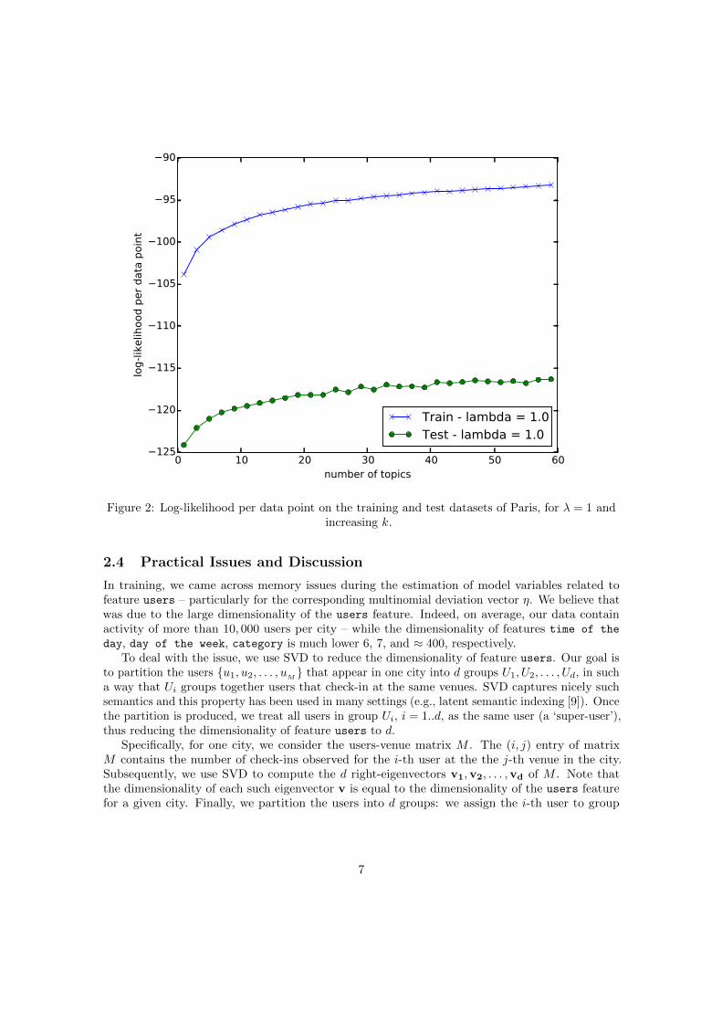
(for η values) performed numerically.To optimize with respect to k and λ, we experiment with a grid of values and select the pair of

values with the best performance on the test set. We found that λ ≈ 1 worked well for all cities weexperimented with, while improvement reached a plateau for values of k near k ≈ 50− 55. Figure 2shows the training plots for the city of Paris; similar patterns are observed for the other cities inthe dataset.

6

0 10 20 30 40 50 60number of topics

125

120

115

110

105

100

95

90

log-l

ikelih

ood p

er

data

poin

t

Train - lambda = 1.0Test - lambda = 1.0

Figure 2: Log-likelihood per data point on the training and test datasets of Paris, for λ = 1 andincreasing k.

2.4 Practical Issues and Discussion

In training, we came across memory issues during the estimation of model variables related tofeature users – particularly for the corresponding multinomial deviation vector η. We believe thatwas due to the large dimensionality of the users feature. Indeed, on average, our data containactivity of more than 10, 000 users per city – while the dimensionality of features time of the

day, day of the week, category is much lower 6, 7, and ≈ 400, respectively.To deal with the issue, we use SVD to reduce the dimensionality of feature users. Our goal is

to partition the users {u1, u2, . . . , uM} that appear in one city into d groups U1, U2, . . . , Ud, in such

a way that Ui groups together users that check-in at the same venues. SVD captures nicely suchsemantics and this property has been used in many settings (e.g., latent semantic indexing [9]). Oncethe partition is produced, we treat all users in group Ui, i = 1..d, as the same user (a ‘super-user’),thus reducing the dimensionality of feature users to d.

Specifically, for one city, we consider the users-venue matrix M . The (i, j) entry of matrixM contains the number of check-ins observed for the i-th user at the the j-th venue in the city.Subsequently, we use SVD to compute the d right-eigenvectors v1,v2, . . . ,vd of M . Note thatthe dimensionality of each such eigenvector v is equal to the dimensionality of the users featurefor a given city. Finally, we partition the users into d groups: we assign the i-th user to group

7

g ∈ {0, 1, . . . , d} such thatg = argmax

j∈{1,2,...,d}{v1[i],v2[i], . . . ,vd[i]}

This provides naturally the partition U1, U2, . . . , Ud we aimed to identify.Note that in our experimentation we employed SVD for a large range of dimensionality values

d ∈ [100, 103] and found that increasing d beyond d = 1000 did not significantly improve the modelperformance. We thus settled for d = 1000.

Flexible Number of Features

The model defined in Section 2.2 is employed on data that exhibit a particular set of categoricalfeatures, as described in Section 2.1. Nevertheless, this does not preclude that the model be appliedon data that exhibit a different (smaller or larger) number of categorical features. Suppose, forexample, that one wishes to train a model that takes into account only the location and category ofvenues, but not the check-in information (time and user of the check-in). A simple way to achievethis is to provide a single data point for each venue. The data point would contain the venueinformation (location and category) and some placeholder value for all the other features. Thisallow us to learn a model only for the category and location of venues. In practice, then, one couldsimply remove non-available features from the model – i.e., one would have vectors β(i) only for thefeatures at hand (see Figure 1) and train on them.

Location

The geographic component of the model we use does not match the notion of neighborhood asconceived in a more administrative sense, e.g., as a set of roads or other boundaries that enclose ageographical area. However, our goal in the paper is not to discover such neighborhoods, but ratherto discover geographical patterns that represent well, in a probabilistic sense, the activity observedin the data at hand. The geographical patterns we look for are associated with more loosely-definedregions, represented by two-dimensional Gaussians. Moreover, note that the model allows regionsto overlap and at the same time accommodate a number of categorical features.

In practice, this means that we might discover topics in the data that have highly overlappinggeographical regions, but are differentiated based on other features. For example, in training themodel, we might discover that there are two topics in the same region – one consisting of venuesthat operate early in the morning, and of venues that operate late in the evening. This is a basicdifference from related work such as [4], that aims to directly partition the area of a city intonon-overlapping regions.

Dataset Biases

One challenge that arises in using Foursquare checkins as our dataset is how to assess whetherthe activity (checkins) recorded in the data are representative of the actual activity in the city.In other words, are Foursquare data representative of what people actually do in the city? Suchan assessment is the material of future work that is beyond the scope of this paper, as it wouldrequire additional technical tools and additional ground-truth data. Until then, we are carefulabout the claims we make about the empirical findings of our method: these empirical findingssolely represent the urban activity contained within the Foursquare dataset.

8

3 Likely and distinctive feature values

Following the learning procedure defined in Section 2, we learn a single model for each city in ourdata. The value of these model instances is that they offer a principled way to answer questionsthat we cannot answer from raw data alone. To provide an example, suppose that an acquaintancefrom abroad visits our city and asks “if I stay at location l of the city, what is the most commonvenue category I find there?”. Raw data do not provide an immediate answer to the question. Theydo allow us, for example, to provide answers of the form “within radius r from l, the most commonvenue category is c with n out of N venues”. However such answers would depend on quantity r,that was not provided as input – and would probably never be, if our friend does not have anyknowledge about the city. Selecting too small a value for r (e.g., a few meters), would make theanswer sensitive to the exact location l; selecting too large a value for r (e.g., a few kilometers),would make the answer insensitive to the exact location l.

The unsupervised learning approach we take allows us to avoid such arbitrary choices in aprincipled manner. It learns topics associated with Gaussian distributions as regions, whose size islearned from the data; and under a model instance I, it allows us to answer our friend’s questionby simply considering the probability

p(category = c|location = l; I)

that at the given location we find a venue of category c, and answering with the category that isassociated with the highest probability value.

Given such model instances, we explore the geographical distribution of venues for the cor-responding cities. Due to space constraints, we provide only a few examples here and provide acomplete list of findings from this section on the project’s webpage1.

Most likely feature value Suppose a venue is placed at a given location loc = (x, y) – what isthe category most likely associated with it? In other words, we are asking for the category thatmaximizes the expression

p(category = c | location = l; I) (4)

that we just discussed above. We use our model to answer this question for New York. The resultsare shown in Figure 3(a). We can ask a similar question for the remaining categorical featuresrepresented in our model. For example, suppose a venue is placed at a given location, what is themost likely time a check-in occurs at that venue? The results for New York are given in Figure 3(b).

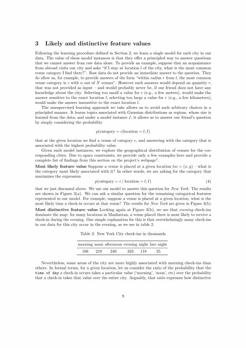
Most distinctive feature value Looking again at Figure 3(b), we see that evening check-insdominate the map: for many locations in Manhattan, a venue placed there is most likely to receive acheck-in during the evening. One simple explanation for this is that overwhelmingly many check-insin our data for this city occur in the evening, as we see in table 2.

Table 2: New York City check-ins in thousands

morning noon afternoon evening night late night

106 219 240 333 118 25

Nevertheless, some areas of the city are more highly associated with morning check-ins thanothers. In formal terms, for a given location, let us consider the ratio of the probability that thetime of day a check-in occurs takes a particular value (‘morning’, ‘noon’, etc) over the probabilitythat a check-in takes that value over the entire city. Arguably, that ratio expresses how distinctive

9

Home (private)

Theater

Office

(a) category

NOON

EVENING

(b) time of day

Thursday

Saturday

Friday

(c) day of week

Figure 3: Most likely category and checkin time of day, day of week across Manhattan.Note that the transparency of each point is equal to the probability that a venue is located at that

point.

that value is for this particular location. Formally, it is expressed as follows.

p(time of day = t | location = l; I)

p(time of day = t | I(5)

For example, suppose that a venue at a particular location loc receives a check-in in the morningwith probability 30%; and that on average across the city venues, a venue would receive a check-inin the morning with probability only 1%. Then, we can say that location loc is associated withvenues that are distinguished for the relatively high frequency of morning check-ins. Figure 4(b)indicates the most distinctive time of check-in across New York. We can ask a similar question forother categorical features. For example, what is the most distinctive category for the same location?The results for New York are shown in Figure 4(a).

4 Feature analysis

In the previous section, we employed the model instance of a city to ask questions about thegeographical distribution of a given feature. In this section, we study the importance of eachfeature in distinguishing the different topics that define a model instance. To further illuminatethe question, let us remember that the model is built upon a set of features {X} and that thedistribution of each feature is allowed to vary across topics. In plain terms, the question we ask isthe following: if we were forced to fix the distribution of feature X across topics, how much wouldthat hurt the predictive performance of the model? This question is important, not just for the

10

Speakeasy

Fried Chicken Joint

Baseball Field

Veterinarian

Steakhouse

Medical Center

(a) category

NIGHT

LATENIGHT

NOON

EVENING

AFTERNOON

MORNING

(b) time of day

Thursday

Saturday

Monday

Sunday

Friday

Wednesday

(c) day of week

Figure 4: Most distinctive category and checkin time of day, day of week across Manhattan.The transparency of each point is equal to the probability that a venue is located at that point.

purposes of feature selection in case one wanted to employ a simpler model, but also because itallows us to suggest on what features future work should be focused, in order to understand betterurban activity.

To be more specific, let us first consider the categorical features in our model: category, users,time of the day, day of the week. Within each topic of a model instance, the distributionβ of each of the aforementioned features deviates from the overall distribution µ by a vector η(Equation 1). To quantify to which extent a single categorical feature X contributes to the varianceacross topics, we perform a simple ablation study. That is, we select the same training set as forour best model, keep the value of parameters k and λ, and train a model instance by fixing the η offeature X equal to zero.

for categorical featureX : set η = 0

Subsequently we compare the log likelihood of both models (the best one and the ablated one) overall the data for the given city and measure the log-likelihood drop between the two. The higherthis drop, the higher the importance of that feature in explaining the variance across topics.

We perform a similar procedure for the location feature. Specifically, for the ablated model,we replace the bivariate Gaussian distribution Gz associated with each model with a distributionG0 that remains fixed across topics. G0 is set to be the mixture of Gaussians Gz across topics z,with mixture proportions equal to topic proportions θz.

for location : set G0 = mixture{Gz, θz}

Results are summarized for all cities in Figure 5. The immediate observation is that users

prominently stand out as a feature and that this is consistent across all cities. This suggests that,

11

at least for the urban activity represented in our dataset, who visits a venue has a more importantrole to play in distinguishing different venues, than where the venues are located and when theyare active. At this point, we should also stress that there is very little overlap in the users that

day of week location category time of day users0

2

4

6

8

10

12

14

16

18

perc

enta

ge o

f log

like

lihoo

d dr

op

Figure 5: Contribution of each feature to the data likelihood. The boxplots summarize how muchthe log likelihood drops once we fix the distribution of a single feature across topics. We observe aconsistent behavior across cities, in that the variance of users across topics is most important for

the predictive performance of the model.

check-in at different cities (see Figure 6). Among the remaining features, location and time of

the day, are consistently more important across cities than day of the week and category.

5 Similar regions across cities

In this section, we address the task of discovering similar regions across different cities. Addressingthis task would be useful, for example, to generate touristic recommendations for people who visita foreign city or generally to develop a better understanding of a foreign city based on knowledgefrom one’s own city. Specifically, we are given the trained models of two (2) cities as input and aimto identify one region from each city so that a similarity measure for the two regions is maximized.Following the conventions of this work, each region is spatially defined in terms of a bivariateGaussian distribution. Moreover, in the interest of simplicity, we consider only cases where thesimilarity measure concerns a single categorical feature. In what follows, we devise a measure toquantify the similarity of two regions and present an algorithm to find similar regions according tothat measure. Then, we describe some aggregate observations from employing this measure on ourdataset.

5.1 Similarity Measure

We start by defining a similarity measure jointsim that has a natural interpretation in our setting.It quantifies (i) how similar the venues of two regions are on average, according to the correspondingmodels, but also (ii) how many venues they contain, according to the model. The rationale for thesecond point is that one wishes to identify regions that have large probability under the model andavoid identifying pairs of tiny regions that are ‘spuriously’ similar.

Let us now define formally the jointsim measure, which operates under the following settings.We are given two model instances, I1 and I2, each corresponding to a city in our data. As explainedin earlier sections of the paper, each model instance describes the distribution of venues in itsrespective city, along with distributions over every features. Moreover, we are given two bivariate

12

AmsterdamAnkaraAntalyaAtlanta

BarcelonaBelo Horizonte

BerlinChicago

FortalezaHelsinkiHouston

Indianapolis

IstanbulKuala Lumpur

LondonLos AngelesMexico City

MoscowNew York

ParisPorto Alegre

Prague

RecifeRio de Janeiro

RomeSalvador

San DiegoSan Francisco

Santiago de ChileSao Paulo

SeattleSingapore

Saint LouisStockholm

Saint PetersburgTokyo

WashingtonYokohama

Amste

rdam

Ankara

Antalya

Atlanta

Barce

lona

BeloHoriz

onte

Berlin

Chicago

Fortalez

a

Helsin

ki

Houston

Indian

apolis

Istan

bul

KualaLum

pur

London

Los Angeles

Mex

icoCity

Mosc

ow

NewYork

Paris

PortoAleg

re

Prague

Recife

Riode Jan

eiroRom

e

Salvad

or

San Dieg

o

San Fra

ncisco

Santia

go de Chile

Sao Pau

lo

Seatt

le

Singap

ore

Sain

t Louis

Stock

holm

Sain

t Petersb

urg

Tokyo

Was

hingto

n

Yokohama

0

3

6

9

12

15

Figure 6: Jaccard coefficient between sets of users that appear in different pairs of cities.

13

model grid_1 grid_5 grid_10 som0.000

0.002

0.004

0.006

0.008

0.010

0.012

0.014jo

ints

im

Figure 7: The jointsim values for the best-matching regions returned by GeoExplore across allpairs of cities, for different sets of base-regions (model, grid-α and SOM).

Gaussian distributions, G1 and G2, each defining one geographic region in the respective modelI1 and I2. To define the similarity between the two regions with respect to feature X (e.g., X =category), we first define a random procedure R(I,G,X). Given a model instance I and a regionG, random procedure R generates a pair of values (x, s), with x ∈ Dom(X) and s ∈ R+. It isdefined as follows.

Definition 1 (R(I,G,X)) Perform the following steps.

• Generate a data point d ∼ I, with location loc = l and feature X value X = x.

• Let s = N (l) be the probability density of G at location l.

• Return the pair (x, s).

In plain terms, random procedure R(I,G,X) picks a random data point from model instance I,and associates it with (1) its value X = x for feature X and (2) the density of region-definingGaussian G. Similarity measure jointsim then answers the question: ‘if random procedure R isapplied on model I1 and region G1, on one hand, and model I2 and region G2, on the other, withrespective output pairs (x1, s1) and (x2, s2), what is the expected value of the expression

s1 · s2 · δx1x2 ,

over possible invocations of procedure R’? In the expression above, δx1x2 is the Kronecker delta –equal to one (1) only when x1 = x2 and zero (0) otherwise. In other words, jointsim combines theanswer of the following two questions: if we consider two random venues, one from each model I1and I2, then (1) what is the probability that they have the same value for feature X, and (2) ifthey do, how much are their locations covered by regions G1 and G2? The measure is formallydefined below:

14

Definition 2 (jointsim) Let (x1, s1) and (x2, s2) be the output of a single invocation of randomprocedure R(I1, G1, X) and R(I2, G2, X), respectively. Similarity jointsim is defined as the expectedvalue

jointsim(G1, G2; I1, I2, X) = ER[s1 · s2 · δx1x2] (6)

We now proceed to provide an analytical expression for jointsim. First, in the interest of simplic-ity, we fix model instances I1, I2 and featureX and write jointsim(G1, G2) = jointsim(G1, G2; I1, I2, X).Let us also write ψi(x, l) to denote the joint probability that model Ii (i ∈ {1, 2}), generates adata point with feature value X = x and location l,

ψi(x|l) = p(X = x, loc = l|Ii),

which can be expanded to

ψi(x|l) = p(X = x, loc = l; Ii)

= p(X = x, loc = l|Ii)=

∑z=1,...,k p(X = x, loc = l, topic = z|Ii)

=∑z=1,...,kNz(l)βz(v)θz

where Nz denotes the Gaussian probability density function for the Gaussian distribution associatedwith the z-th topic, z = 1, . . . , k, of model Ii. Finally, for locations l1 and l2, let us write h(l1, l2)for the inner-product function

h(l1, l2) =∑

x∈Dom(X)

ψ1(x, l1)ψ2(x, l2). (7)

With the notational conventions above, we now provide an analytical expression for jointsim.

jointsim(G1, G2) =

∫l1,l2

N1(l1)N2(l2)h(l1, l2)dl1dl2 (8)

Note that, in equation (8), N1 and N2 denote the probability density functions of Gaussians G1

and G2, respectively. Moreover, we approximate the integral of equation (8) with a discrete sumapproximation over a 100× 100 grid on each model.

Having defined our similarity measures, let us consider the corresponding maximization problem.

Problem 2 Consider two models I1, I2, and feature X. Identify two bivariate Gaussians G1, G2,such that jointsim(G1, G2) is maximized.

Problem 2 has two intuitive properties:

• all other things being equal, it favors regions G1 and G2 that cover areas with high probabilitymass according to models I1, I2,

• all other things being equal, it favors regions G1 and G2 that cover areas where data points areassociated with similar feature distributions.

To put in plain terms, Problem 2 favors regions that correspond to areas of many and similardata points. This is seen also in equations (7) and (8). Indeed, they take into account the similarityof data points (venues) in terms of feature X at locations within the two regions, but they alsotake into account the probability mass assigned to those regions by models I1 and I2. This makesProblem 2 appropriate to consider in cases when one does not have prior restrictions or preferencesfor the candidate regions that would comprise an optimal solution and at the same time wouldlike to avoid spurious solutions, i.e., pairs of regions that are very similar, but that cover too smallprobability mass of the respective models.

15

5.2 Best-First Search for jointsim

To the best of our knowledge, the problem of identifying similar regions across cities has not beendefined formally before within a probabilistic framework. In this section, we also propose the firstalgorithm, GeoExplore, to approach Problem 2. Algorithm GeoExplore follows a typical best-firstexploration scheme and comprises of the following two phases. Its first phase consists of one step:it begins with a candidate collection of regions G1 and G2 for each side (let us call them ‘baseregions’) and evaluates all pairwise similarities jointsim(G1, G2), for G1 ∈ G1, G2 ∈ G2. Itssecond phase consists of the remaining steps: it explores the possibility to improve the currentlybest jointsim measure by combining previously considered regions. This is motivated by the factthat Problem 2 favors regions of larger probability mass, and therefore combined regions mightyield better jointsim values.

Pseudocode for GeoExplore is shown in Algorithm 1. It repeats a three-steps Retrieve - Update- Expand procedure for each step. During Retrieve, the algorithm retrieves the next candidatesolution for Problem 2. Each candidate solution comes in the form of a triplet; two Gaussiansand their jointsim score. During Update, the algorithm updates the score of the best-matchingpair, if a better pair has just been retrieved. Finally, during Expand, the algorithm expands thelatest retrieved Gaussians to form Gaussians from each side, and thus new candidate solutions forProblem 2. Subroutine expand(G, I) operates as follows:

• When G is not specified (i.e., G = NULL in Algorithm 1), then expand simply returns theset of base regions G. This case occurs during the first expansions only. Moreover, each baseregion Gi ∈ G is associated with positive weight wi, either specified as input, or set to 1/‖G‖by default.

• When G = Gi for some Gi ∈ G, then expand returns the set of Gaussians {Gi}⋃{Gi∪Gj ;Gj ∈

G, j 6= i}, where Gi ∪Gj is defined as the best Gaussian-fit to the mixture model determinedby [Gi, Gj ], with respective proportions (wi, wj). The intuition for this step is that we expandthe best-performing pair of Gaussians by combining them with other base Gaussians.

• In a recursive fashion, when G = Gi ∪Gi′ . . . Gi′′ , then expand returns the set of Gaussians{G}

⋃{G ∪ Gj ;Gj ∈ G, j 6= i, i′, . . . , i′′} each defined as the best Gaussian-fit to the mixture

model determined by [G, Gj ], with respective proportions (wi + wi′ + . . .+ wi′′ , wj).

Note that in practice, to prevent the algorithm from exploring the combinatorially large space,we terminate GeoExplore after a number R of while loops. If k1, k2 are the number of topicsin the two model instances, we perform O(k1 + k2) expansions as well as O(k1 · k2) jointsim

evaluations in each loop. If the respective running-time costs of the operations are c1 = cexpansionand c2 = cjointsim, the total running time of the algorithm is O(R · ((k1 + k2)c1) + k1k2c2).

5.3 Empirical performance

We employed GeoExplore with R = 5 expansions on all pairs of cities in our dataset (Section 2.1)and report the jointsim values returned for different base region collections. Specifically, weexperimented with the following collections of base regions:

Model We simply used as collections G1, G2 the Gaussians associated with the respective topicsin the input model I1, I2, and assigned to each Gaussian a weight equal to the respective θparameter value found in the model.

Grid-a We used as collections G1, G2 Gaussians that covered in a grid-like fashion the respectivecities, each with size equal to 1/a the size of the median size of Gaussians found in model I1,I2.

16

Algorithm 1 GeoExplore

Input: models I1 and I2, base regions G1, G2

Output: Best Pair G1, G2

# INITIALIZEBestG1 = NULL, BestG2 = NULL, BestScore = 0H = MaxHeap()# Initialize max-heap with empty solution, zero scorePush(BestG1, BestG2, BestScore) to H

while H is Not Empty do# RETRIEVE top solution in max-heapPop (G1, G2, Score) from H# UPDATE best solutionif Score > BestScore then

BestG1 = G1, BestG2 = G2, BestScore = Scoreend if# EXPAND retrieved solutionfor Ga, Gb in expand(G1), expand(G2) 6= G1, G2 do

Score = jointsim(Ga, Gb|I1, I2)Push (Ga, Gb, Score) to H

end forend whilereturn best pair

Table 3: The improvement rate for each value of R, i.e., the fraction of times that the algorithmfound an improved solution out of all the times it reached that round.

R 1 2 3 4 5

improvement rate 53.0% 2.7% 2.3% 1.8% 1.6%

SOM We employed the method of Self Organized Maps [6] to generate a set of closed regions thatcover each city. Subsequently, for each such region, we find the smallest bivariate Gaussianso that the entire region is enclosed within two standard deviations of the Gaussian in eachdirection. We use these Gaussians as collections G1, G2 and employ GeoExplore.

The results are shown in Figure 7. We observe that using the model Gaussians as our base regionsleads to better performance compared with the grid baselines.

The reason we stopped expansions at R = 5 was that beyond that point we found it was veryunlikely to obtain an expansion that led to an improvement – see Table 3.

Finally, in Figure 8, we show two examples of pairs of regions with high jointsim score, whichwe discovered by running GeoExplore. In both cases, the first region is in San Francisco. As wecan see in blue on 8(a), it covers the Mission district and a part of the downtown area. Amongall the other cities in our data, GeoExplore found that the region 34 of New York (shown in greenon 8(c) and covering the city of Hoboken and West Village was most similar to it in the sense ofjointsim, as well as a region in Rome that covers the district of Monte Sacro (shown in red on8(d)). As explained earlier, these regions are not spuriously small and since we measure similaritywith respect to the category feature, it is not surprising that they have similar distributions of

17

(a) San Francisco: Missionand Downtown

0 5 10 15 20 25 30 35Percentage of venues

Entertainment

Education

Food

Nightlife

Outdoors

Shop and Service

Professional

Residence

Transport

Rome, Monte SacroSan Francisco, Mission & DowntownNew York, Hoboken & West Village

(b) Distributions of VenueCategories.

(c) New York: Hobokenand West Village

(d) Rome: Monte Sacro

Figure 8: Examples of regions identified as similar by GeoExplore.

checkins among Foursquare top categories – i.e., predominantly at Food, but also Shops and otherProfessional venues, as one can see on 8(b).

6 Comparison with previous approaches

In this section, we compare empirically our approach with previous works. Ideally, our comparisonwould be with works that address the same task as this paper, i.e., model the distribution of venuesacross a city. In such a case, we would have a natural and direct measure of comparison, namelythe predictive performance of each model in terms of log-likelihood. However, to the best of ourknowledge, no such work is readily available. Therefore, our comparison is with previous worksthat (i) address slightly different tasks and (ii) do not make explicit use of a probabilistic model.Nevertheless, the comparison serves as a ‘sanity check’ for our approach and helps demonstratebetter the proposed technique.

We compare with two methods that provide publicly available results, namely Livehoods5 andHoodsquare6. Their results cover three large US cities that also appear in our dataset. Bothmethods use Foursquare data and output a geographical clustering of venues within a city, witheach such cluster defining one region on the map of the city. In the case of Livehoods [4], theclusters are obtained through spectral clustering on a nearest-neighbor graph over venues, wherethe edge weights quantify the volume of visitors who check-in at both adjacent venues. In thecase of Hoodsquare [5], clusters are obtained by employing the OPTICS clustering algorithm onvenues, using a number of venue features (location, category, peak time of activity during the day,and a binary touristic indicator). Furthermore, we also implement the method of [6]. Although ituses Twitter data to classify land usage, it is also a simple non-parametric method based on SelfOrganized Maps (referred to as SOM hereafter) to segment the city by clustering geolocated tweets.

To compare, we perform the following procedure. First, we obtain the clusters returned byeach method. We interpret each of those clusters as a region that belongs to one topic, in thesense that we have been using the term in the context of our model. To map them to our setting,we approximate the shape of each region with the smallest bivariate Gaussian so that the entireregion is enclosed within two standard deviations of the Gaussian in each direction (see Figure 9for the visual results of this approximation in San Francisco). In this way, we obtain a number k of

5http://livehoods.org/maps6http://pizza.cl.cam.ac.uk/hoodsquare

18

Gaussians from each method. We then train an instance of our model on our data, using the samenumber k of topics, and keeping the Gaussians associated with each topic fixed to the Gaussiansextracted with the aforementioned steps. As in previous sections of the paper, we hold out 20% ofthe data as test set, on which we evaluate the log-likelihood of each learned model instance.

The log-likelihood achieved by the different models is shown in the first row of Table 4. As onecan see there, the results based on our model perform better in predicting the test set. This isnot surprising, since our approach optimizes predictive accuracy directly. Nevertheless, the resultsprovide evidence that our approach works reasonably well for the task it was designed to address.

To further quantify the differences between the four approaches, we report additional quantitiesfrom the learned models, described below. Essentially, those quantities capture how distinct theidentified regions of each model are in terms of the associated features.Mean Feature Entropy We consider each categorical feature separately and, for each topicregion in the respective model of the four approaches, we measure the entropy of the respectivemultinomial distribution β. Intuitively, we would like the regions that constitute our model instancesto capture the variance of the various features across the city. Therefore, we would like the βdistributions of the model instances to have lower entropy (i.e., be farther from uniform). Table4 reports the mean entropy of β across regions for each categorical feature and for each of themethods in the three US cities. The relevant lines in the table are the ones labelled ‘mean [feature]entropy’. As one can confirm, in the majority of cases the model instance based on our methodreturns β distributions of lower entropy.Jensen–Shannon Divergence from City Average Another way to quantify the distinctive-ness of the various regions is to measure the distance of the β distribution of each feature and topicin the model from the average distribution µ for the same feature across the city. One principledapproach to quantify this difference is to use Jensen–Shannon divergence JSD(β, µ), a symmetrizedversion of the Kullback–Leibler divergence KL(P ‖ Q) defined as:

JSD(β, µ) = 0.5 ·KL(β ‖ (β + µ)/2) + 0.5 ·KL(µ ‖ (β + µ)/2))

Intuitively, it is desirable for β distributions of different topics to differ from average city behavioras captured by µ distributions. Table 4 reports the average Jensen–Shannon divergence across thetopics for each categorical feature, city, and method. The relevant lines in the table are the oneslabelled ‘[feature] JSD from city’. Again, in the majority of cases, the model instance based on ourmethod returns β distributions that differ more from city average distribution than the methodswe compare with.

To summarize our findings from Table 4, our model has better predictive performance, whilegenerally identifying topic regions that are more distinct with each other and further from average,despite their high overlap. The results thus provide evidence that our approach discovers regionswith desirable properties.

7 Related Work

Urban Computing is an active area of research, partially due to the increasing volume of digitaldata related to human activity and the potential to use such data to improve life in cities. Below,we discuss related works that either address a similar task (finding geographical structure in cityactivity) or use a similar approach to ours to address different tasks. To the best of our knowledge,we are the first to employ a fully probabilistic approach to this task – and thus discuss further theconcept of sparse modeling. Finally, we discuss other Urban Computing tasks more loosely relatedto our work.

19

Table 4: Comparison in San Francisco, New York and Seattle between our model (with @k topics),SOM, Livehoods (LH) and Hoodsquare (HS, which has no neighborhoods available in Seattle).The last abbreviation, JSD, stands for the average Jensen–Shannon divergence between regions

and city-wide distributions of the four features we consider: category, users, dayOfWeek andtimeOfDay. Each group of two adjacent columns is a comparison between a competing method

and our model. The arrow after the name of each measure indicates whether higher or lowervalues are better.

San Francisco New York SeattleSOM Us@22 HS Us@13 LH Us@39 SOM Us@18 HS Us@12 LH Us@68 SOM Us@43 LH Us@64

likelihood per venue ↗ -198.2 -197.4 -202.9 -199.2 -197.0 -195.7 -270.4 -268.4 -335.3 -271.2 -264.2 -262.4 -175.6 -174.5 -174.7 -172.9

mean category entropy ↘ 4.786 4.740 4.959 4.754 4.808 4.808 4.847 4.737 4.905 4.784 4.864 4.815 5.178 5.196 5.141 5.216category JSD from city ↗ 0.070 0.079 0.053 0.066 0.066 0.059 0.061 0.079 0.051 0.070 0.056 0.056 0.004 0.004 0.009 0.001

mean dayOfWeek entropy ↘ 1.896 1.900 1.908 1.912 1.892 1.900 1.928 1.924 1.924 1.932 1.916 1.916 1.910 1.905 1.899 1.865dayOfWeek JSD from city ↗ 0.011 0.011 0.007 0.008 0.011 0.011 0.004 0.005 0.004 0.004 0.007 0.007 0.007 0.007 0.009 0.016

mean timeOfDay entropy ↘ 1.437 1.424 1.488 1.483 1.428 1.416 1.589 1.550 1.536 1.561 1.540 1.540 1.476 1.442 1.475 1.377timeOfDay JSD from city ↗ 0.030 0.033 0.018 0.024 0.031 0.035 0.014 0.024 0.014 0.023 0.022 0.024 0.025 0.033 0.025 0.048

mean user entropy ↘ 5.550 5.544 5.610 5.328 5.521 5.407 5.338 5.386 5.931 5.370 5.221 4.947 5.069 5.178 5.128 5.088user JSD from city ↗ 0.176 0.176 0.160 0.204 0.175 0.186 0.212 0.206 0.101 0.203 0.209 0.234 0.198 0.178 0.183 0.176

7.1 Finding Structure in Urban Activity

Finding cohesive geographical regions within cities has been attempted using a variety of datasources: public transport and taxi trajectories [10, 11], cellphone activity [12], geotagged tweets [6],social interactions [13] or types of buildings [14].

In that context, Location Based Social Networks (LBSNs) have also proven a rich source ofdata and were used by recent works. For instance, [4] collects checkins and build a m-nearestspatial neighbors graph of venues, with edges weighted by the cosine similarity of both venues’ userdistribution. The regions are the spectral clusters of this graph. Using similar data, [5] describesvenues by category, peak time activity and a binary touristic indicator. Venues are clustered inhotspots along all these dimensions by the OPTICS algorithm. The city is divided into a grid,with cells described by their hotspot density for each feature. Finally, similar cells are iterativelyclustered into regions. Like us, [15] considers venues to be essential in defining regions. The city isdivided into a grid of cells with the goal of assigning each cell a category label in a way that is asspecific as possible while being locally homogeneous. This is done through a bottom-up clusteringwhich greedily merge neighboring cells to improve a cost function formalizing this trade off.

Whereas these results are evaluated with user interviews and build upon well known algorithmictechniques, they rely on ad-hoc modeling decisions (such as graph construction and grid granularity)that do not derive directly from the data, thus questioning the statistical significance of the obtainedresults. Furthermore, because the clustering is not guided simultaneously by all the available datafeatures, such as time and aspects other than venue category, important information might be goingamiss in those approaches.

On the other hand, there are works that take a probabilistic approach, although their aim isdifferent than ours. For instance, [16] assigns venues to a grid and runs Latent Dirichlet Allocation(LDA) on their categories. However it does not output explicit regions, and the grid is a coarseapproximation for using spatial information. Instead, [17] fixes a number K of localized topics tobe discovered, as well as a set of N Gaussian spatial regions. Each region has a topic distributionand each topic is a multinomial distribution over all possible Flickr photos tags. Relaxing severalassumptions, notably the Gaussian shape, [18] extends Hierarchical Dirichlet Process to spatial

20

(a) Hoodsquare (b) Our method (c) Livehoods

(d) SOM

Figure 9: In San Francisco, the second panel shows the top 12 regions (sorted by decreasingweight) we obtained with our probabilistic model. On the left, Hoodsquare regions are extracted

from their website and transformed into Gaussians. On the right are the same picture forLivehoods and SOM. All methods show that the city activity occurs mainly downtown but it alsohighlights differences between approaches. For instance, although Livehoods exhibits some overlap,

it is only due to the Gaussian conversion whereas we do not restrain venues to serve a singlefunction in a single region by construction, but only let that happens if the data support it.

data, giving rise to an almost fully non-parametric model (as the number of regions still needs to beset manually). While such methods bear similarity with ours, the domain of application presentedby their authors forbids direct comparisons.

Closer to the task of finding regions, [19] performs LDA on checkins in New York. The fiveresulting topics are called urban activities, and venues are clustered by their topic proportion acrosstime. Contrary to us, this clustering does not produce clearly defined regions, since it is done as apost processing step. Indeed, their LDA model does not incorporate a spatial dimension. Movingfrom checkins to a dataset of 8 millions Flickr geotagged photos, [20] probabilistically assigns tagsto one of the three levels of a spatial hierarchy, where each node is associated with a multinomialdistribution over tags. Regions can then be characterized by finding their most descriptive tags.

7.2 Sparse Topic Model

We now present related applications of the Sparse additive generative model on spatial data. Theoriginal SAGE paper [3] evaluates its model effectiveness on the task of predicting the localizationof twitter users by learning not only topics about words but also about metadata (i.e., in whichregion was the tweet written) and shows good accuracy. Later, a simplified version of it was usedto find regions which exhibit geolocated idioms [21]. It is possible to better model user location bybuilding a hierarchy of regions [22]. Even though the sparsity of model is well suited to the sparsityof textual data, note that methods which do not use topic modelling give competitive results interms of accuracy [23, 24].

21

Another task hindered by data sparsity and which benefits from modeling user preferences isspatial item recommendation. The interested reader will find many examples exploiting LBSNin a recent survey [25], but here we give a taste of two approaches inspired by SAGE. In bothcases, topics are distributions over words and venues. Each user is endowed with her own topic,and so to are each region. [26] uses SAGE to model user topics as a variation from the overallglobal distribution. To improve out of town recommendation, [27] assigns to regions both local andtourist topics. Learning such high number of parameters is made possible by combining SAGE anda hierarchical model called spatial pyramid.

7.3 Other Urban Computing Problems

After finding regions in a city, a natural task is to compare them, within or across cities. One mightalso look at different granularity to perform such urban comparisons, whether points of interest orcities as a whole. Finally, one might focus on users and model their preferences through mobilitydata.

Comparing regions We saw that one way to compare regions is to assign them descriptivetags [20]. Others have looked at a more information retrieval approach [28], while in [7], authorscollect data from Foursquare and Flickr to associate venues with a features vector summarizingtheir time activity, their surroundings, their category and their popularity. They then define thesimilarity between two regions as the Earth Mover Distance between the two sets of venues featurevectors they contain. Finally they devise a pruning and clustering strategy to find similar regionsbetween cities.

Finding points of interest Regions are only one subdivision of the city, another one arepoints of interest, which are locations where the user activity show some specificities. Geotaggedphotos can be mined to extract the semantics of such locations [29, 30, 31, 32]. As a representativeexample, [33] compares various spatial methods to discover small areas in San Francisco where onephoto tag appears in burst. GPS trajectories provide useful information as well [34, 35, 36]. Forinstance, [37] extracts stay points from car GPS data and assess their significance by how manyvisitors go there, how far they traveled to reach them and how long they stay.

Comparing cities This has been done by comparing the spatial distribution of human hotspotsusing call data [38], the call data profile themselves [39], the distribution of venues category atvarious scales [40], or by building a network of city from urban residents mobility flow and computingcentrality measures [41].

Clustering users With venues, users are the other side of the coin of what defines a regionin a city, and some works have mine their activities to extract meaningful groups. For instance,[42] clusters users by the similarity of their venues category transition probability matrix. Anotherapproach is to consider users as document, checkins as word and apply LDA, thus revealing cohesivecommunities [43] and describing people lifestyle [44].

One can find other applications of Urban Computing in related literature surveys [1, 45].

8 Conclusions

In this work, we made use of a probabilistic model to reveal how venues are distributed in cities interms of several features. As most habitants of a city do not visit most of the available venues, wecope with the induced sparsity by adapting the sparse modeling approach of [3] to data at hand.Fitting our model to a large dataset of more than 11 million checkins in 40 cities around the world,we show the insights provided by such an unsupervised approach.

First, using the extracted model instances, we calculated the probability distribution of a singlefeature conditioned on the location in the city. This enabled us to construct a heatmap of that

22

feature to highlight what feature values are most likely and distinctive at different locations withina city.

Secondly, we described a principled approach to quantify the importance of different featureswithin the trained models. Whereas all features contribute, we discovered that the most definingfeature for the components uncovered by the model is the visitors of venues. This finding suggeststhat further analysis of user behavior is a promising direction for extracting additional insights.

Third, after focusing on the various regions of a single city, we used the extracted model instancesto find the most two similar regions between two cities, a task which was previously attemptedwith a more heuristic approach [7]. This time we also benefit of the solid theoretical grounds ofprobabilistic models to define a principled measure of similarity and we describe a procedure togreedily find two regions maximizing measure. We illustrate this matching process with anecdotalevidence in several cities.

Finally, we compare our approach with previous approaches that provide similar output andshow that our regions are both more consistent with the data (in terms of predictive performance)and have more sharply defined characteristics, meaning they are easier to distinguish from oneanother.

A review of recent related works in the Urban Computing field suggests that whereas the area isactive and that understanding urban activities is a worthy endeavour which benefits from geotaggeddata, it can be pushed further by the use of probabilistic models, as such models come with greatinterpretative power.

Looking beyond this paper, there are further directions in which we can improve our discoveryprocess, providing additional interpretations along the way:

• The first direction is to use a complementary evaluation process, one that would involve moreclosely users, since we show they are the main actor of the regions we discover. For instance,this could take the form of interviews. The purpose of this would be to identify and correct, ifany, significant biases that are embodied in particular datasets (Foursquare activity, in ourcase). One major difficulty, however, lies in finding local experts who have good knowledge ofthe structure and activity of each city.

• The model itself could also be extended, for instance by incorporating hierarchies of regions.This would both provide more structure to our results and allow us to apply our method tolarger geographical area while keeping sparsity and runtime under control. Hierarchy is awell studied concept in both spatial data mining and topic modelling [46] and thus we areconfident this would be a feasible improvement. Another direction would be to incorporateadditional features into the model (e.g., continuous features)

• Just as natural landscapes change with time, whether because of the day/night cycle or thepassing of seasons, so do cities. It is not far fetched to imagine than coastal areas of Barcelonaor San Francisco witness different patterns of activities in the winter than in the summer.Again, following the time evolution of topics has been addressed in different settings [47].

Acknowledgements

This work is supported by the European Community’s H2020 Program under the scheme ‘INFRAIA-1-2014-2015: Research Infrastructures’, grant agreement #654024 ‘SoBigData: Social Mining &Big Data Ecosystem’.

References

[1] Y. Zheng, L. Capra, O. Wolfson, and H. Yang, “Urban Computing: Concepts, Methodologies,and Applications,” ACM Transaction on Intelligent Systems and Technology, vol. 5, no. 3, pp.38:1–38:55, 2014.

23

[2] “World Urbanization Prospects, the 2014 Revision: Highlights,” United Nations, Departmentof Economic and Social Affairs, Population Division, New-York, Tech. Rep., 2014.

[3] J. Eisenstein, A. Ahmed, and E. P. Xing, “Sparse Additive Generative Models of Text,” inICML, Seattle, WA, 2011, pp. 1041–1048.

[4] J. Cranshaw, J. I. Hong, and N. Sadeh, “The livehoods project: Utilizing social media tounderstand the dynamics of a city,” in ICWSM, 2012, pp. 58–65.

[5] A. X. Zhang, A. Noulas, S. Scellato, and C. Mascolo, “Hoodsquare: Modeling and recommendingneighborhoods in location-based social networks,” in ASE/IEEE SocialCom, 2013, pp. 69–74.

[6] V. Frias-Martinez and E. Frias-Martinez, “Spectral clustering for sensing urban land use usingTwitter activity,” Engineering Applications of Artificial Intelligence, vol. 35, pp. 237–245,2014.

[7] G. Le Falher, Gionis Aristides, and M. Mathioudakis, “Where Is the Soho of Rome? Measuresand Algorithms for Finding Similar Neighborhoods in Cities,” in ICWSM, Oxford, 2015.

[8] J. O. Berger and D. Sun, “Objective priors for the bivariate normal model,” The Annals ofStatistics, pp. 963–982, 2008.

[9] S. C. Deerwester, S. T. Dumais, T. K. Landauer, G. W. Furnas, and R. A. Harshman, “Indexingby latent semantic analysis,” JAsIs, vol. 41, no. 6, pp. 391–407, 1990.

[10] N. J. Yuan, Y. Zheng, X. Xie, Y. Wang, K. Zheng, and H. Xiong, “Discovering UrbanFunctional Zones Using Latent Activity Trajectories,” Knowledge and Data Engineering, IEEETransactions on, vol. 27, no. 3, pp. 712–725, 2015.

[11] Jichang Zhao, Ruiwen Li, X. Liang, and K. Xu, “Segmentation and evolution of urban areasin beijing: A view from mobility data of massive individuals,” in Proceedings of the 12thInternational Conference on Service Systems and Service Management (ICSSSM), 2015.

[12] J. L. Toole, M. Ulm, M. C. Gonzalez, and D. Bauer, “Inferring Land Use from Mobile PhoneActivity,” in UrbComp, New York, NY, USA, 2012, pp. 1–8.

[13] J. R. Hipp, R. W. Faris, and A. Boessen, “Measuring ‘neighborhood’: Constructing networkneighborhoods,” Social Networks, vol. 34, no. 1, pp. 128–140, 2012.

[14] Z. Cao, S. Wang, G. Forestier, A. Puissant, and C. F. Eick, “Analyzing the Composition ofCities Using Spatial Clustering,” in UrbComp, New York, NY, USA, 2013, pp. 14:1–14:8.

[15] C. Vaca, D. Quercia, F. Bonchi, and P. Fraternali, “Taxonomy-Based Discovery and Annotationof Functional Areas in the City,” in ICWSM, 2015, pp. 445–453.

[16] J. Cranshaw and T. Yano, “Seeing a home away from the home: Distilling proto-neighborhoodsfrom incidental data with Latent Topic Modeling,” in NIPS’10 Workshop of ComputationalSocial Science and the Wisdom of the Crowds, 2010.

[17] Z. Yin, L. Cao, J. Han, C. Zhai, and T. Huang, “Geographical Topic Discovery and Comparison,”in WWW, 2011, pp. 247–256.

[18] C. C. Kling, J. Kunegis, S. Sizov, and S. Staab, “Detecting non-gaussian geographical topicsin tagged photo collections,” in WSDM, 2014, pp. 603–612.

24

[19] F. Kling and A. Pozdnoukhov, “When a city tells a story: urban topic analysis,” in SIGSPA-TIAL, 2012, pp. 482–485.

[20] M. Kafsi, H. Cramer, B. Thomee, and D. A. Shamma, “Describing and UnderstandingNeighborhood Characteristics through Online Social Media,” in WWW, Florence, 2015, pp.549–559.

[21] J. Eisenstein, “Written dialect variation in online social media,” in Handbook of Dialectology,2015.

[22] A. Ahmed, L. Hong, and A. J. Smola, “Hierarchical Geographical Modeling of User Locationsfrom Social Media Posts,” in WWW, Republic and Canton of Geneva, Switzerland, 2013, pp.25–36.

[23] R. Priedhorsky, A. Culotta, and S. Y. Del Valle, “Inferring the Origin Locations of Tweets withQuantitative Confidence,” in Proceedings of the 17th ACM Conference on Computer SupportedCooperative Work & Social Computing, New York, NY, USA, 2014, pp. 1523–1536.

[24] D. Flatow, M. Naaman, K. E. Xie, Y. Volkovich, and Y. Kanza, “On the Accuracy of Hyper-local Geotagging of Social Media Content,” in Proceedings of the Eighth ACM InternationalConference on Web Search and Data Mining, New York, NY, USA, 2015, pp. 127–136.

[25] J. Bao, Y. Zheng, D. Wilkie, and M. Mokbel, “Recommendations in location-based socialnetworks: a survey,” GeoInformatica, vol. 19, no. 3, pp. 525–565, 2015.

[26] B. Hu and M. Ester, “Spatial Topic Modeling in Online Social Media for Location Recommen-dation,” in Proceedings of the 7th ACM Conference on Recommender Systems, New York, NY,USA, 2013, pp. 25–32.

[27] W. Wang, H. Yin, L. Chen, Y. Sun, S. Sadiq, and X. Zhou, “Geo-SAGE: A GeographicalSparse Additive Generative Model for Spatial Item Recommendation,” in KDD, New York,New York, USA, 2015, pp. 1255–1264.

[28] C. Sheng, Y. Zheng, W. Hsu, M. Lee, and X. Xie, “Answering Top-k Similar Region Queries,”in Database Systems for Advanced Applications, 2010, vol. 5981, pp. 186–201.

[29] D.-P. Deng, T.-R. Chuang, and R. Lemmens, “Conceptualization of place via spatial clusteringand co-occurrence analysis,” in Proceedings of the 2009 International Workshop on LocationBased Social Networks, New York, New York, USA, 2009, pp. 49–56.

[30] M. Shirai, M. Hirota, S. Yokoyama, N. Fukuta, and H. Ishikawa, “Discovering MultipleHotSpots Using Geo-tagged Photographs,” in Proceedings of the 20th International Conferenceon Advances in Geographic Information Systems, 2012, pp. 490–493.

[31] R. Feick and C. Robertson, “A multi-scale approach to exploring urban places in geotaggedphotographs,” Computers, Environment and Urban Systems, 2014.

[32] Y. Hu, S. Gao, K. Janowicz, B. Yu, W. Li, and S. Prasad, “Extracting and understandingurban areas of interest using geotagged photos,” Computers, Environment and Urban Systems,vol. 54, pp. 240–254, 2015.

[33] T. Rattenbury and M. Naaman, “Methods for extracting place semantics from Flickr tags,”ACM Transactions on the Web, vol. 3, no. 1, pp. 1–30, 2009.

25

[34] M. R. Uddin, C. Ravishankar, and V. J. Tsotras, “Finding Regions of Interest from TrajectoryData,” in 2011 IEEE 12th International Conference on Mobile Data Management, vol. 1, 2011,pp. 39–48.

[35] C. Zhang, J. Han, L. Shou, J. Lu, and T. L. Porta, “Splitter: Mining Fine-Grained SequentialPatterns in Semantic Trajectories,” Proceedings of the VLDB Endowment, vol. 7, no. 9, pp.769–780, 2014.

[36] C. Parent, S. Spaccapietra, C. Renso, G. Andrienko, N. Andrienko, V. Bogorny, M. L. Damiani,A. Gkoulalas-Divanis, J. Macedo, N. Pelekis, Y. Theodoridis, and Z. Yan, “Semantic TrajectoriesModeling and Analysis,” ACM Comput. Surv., vol. 45, no. 4, pp. 42:1–42:32, 2013.

[37] X. Cao, G. Cong, and C. S. Jensen, “Mining significant semantic locations from GPS data,”Proceedings of the VLDB Endowment, vol. 3, no. 1-2, pp. 1009–1020, 2010.

[38] T. Louail, M. Lenormand, O. G. Cantu Ros, M. Picornell, R. Herranz, E. Frias-Martinez, J. J.Ramasco, and M. Barthelemy, “From mobile phone data to the spatial structure of cities,”Scientific Reports, vol. 4, 2014.

[39] S. Grauwin, S. Sobolevsky, S. Moritz, I. Godor, and C. Ratti, “Towards a comparative scienceof cities: Using mobile traffic records in new york, london, and hong kong,” in ComputationalApproaches for Urban Environments, 2015, vol. 13, pp. 363–387.

[40] D. Preotctiuc-Pietro, J. Cranshaw, and T. Yano, “Exploring Venue-based City-to-city SimilarityMeasures,” in UrbComp, New York, NY, USA, 2013, pp. 16:1–16:4.

[41] M. Lenormand, B. Goncalves, A. Tugores, and J. J. Ramasco, “Human diffusion and cityinfluence,” Journal of The Royal Society Interface, vol. 12, no. 109, 2015.

[42] D. Preotiuc-Pietro and T. Cohn, “Mining user behaviours: A study of check-in patterns inlocation based social networks,” in Proceedings of the 5th Annual ACM Web Science Conference,New York, NY, USA, 2013, pp. 306–315.

[43] K. Joseph, C. H. Tan, and K. M. Carley, “Beyond ‘Local’, ‘Categories’ and ‘Friends’: ClusteringFoursquare Users with Latent ‘Topics’,” in Proceedings of the 2012 ACM Conference onUbiquitous Computing, New York, NY, USA, 2012, pp. 919–926.

[44] N. J. Yuan, F. Zhang, D. Lian, K. Zheng, S. Yu, and X. Xie, “We Know How You Live:Exploring the Spectrum of Urban Lifestyles,” in Proceedings of the First ACM Conference onOnline Social Networks, New York, NY, USA, 2013, pp. 3–14.

[45] D. Tasse and J. Hong, “Using Social Media Data to Understand Cities,” in Proceedings ofNSF Workshop on Big Data and Urban Informatics, 2014.

[46] D. M. Blei, T. L. Griffiths, and M. I. Jordan, “The nested chinese restaurant process andbayesian nonparametric inference of topic hierarchies,” J. ACM, vol. 57, no. 2, pp. 7:1–7:30,2010.

[47] D. M. Blei and J. D. Lafferty, “Dynamic topic models,” in ICML, 2006, pp. 113–120.

26