Modelling a Tidal Turbine in Unsteady Flow

Simon Gant and Tim StallardSchool of Mechanical, Aerospace and Civil Engineering, University of Manchester

Manchester, UK

ABSTRACT

A brief review of the literature is provided on the characteristics of marine currents and the approaches used for simulating tidal turbines. The feasibility of using CFD models to simulate time-dependent turbulent flow around a tidal turbine is then explored. Two different approaches for specifying the structure of the turbulent inflow conditions in CFD models are compared: the von Kármán spectral approach and the Synthetic Eddy Method (SEM) of Jarrin et al. (2006). The former model is commonly employed in the wind industry and is coded into Garrad Hassan’s Tidal Bladed and NREL’s TurbSim. Different approaches are also tested for decomposing the turbulence at the inlet into resolved and modelled components. The results from these tests indicate that the turbulence produced using the SEM inlet conditions is slightly less susceptible to decay with downstream distance than the von Kármán approach provided that the modelled turbulent kinetic energy accounts for only a small fraction of the total turbulence energy.

Simulations of the unsteady flow around a tidal turbine, represented here as a simple porous disc, provide some insight into the effect of large-scale flow oscillations on the wake of the turbine. The wake structures obtained from unsteady CFD simulations are compared to those obtained using a steady approach. The results indicate that the presence of large coherent turbulent structures in the incident flow field produces a shorter wake than predicted by steady flow simulations.

This work represents the first stage in the development of a unified model which will couple meta-scale simulations of flow in an estuary or complete channel to detailed small-scale simulations of the flow around tidal turbine devices.

KEY WORDS: Tidal Stream Energy; Tidal Turbine; Turbulence; CFD; Unsteady Flow.

INTRODUCTION

The motivation for studying the wake of horizontal axis tidal stream turbines is to understand how device proximity influences both net power output from devices in an array and individual device loading. Over the last decade interest in tidal stream devices has grown rapidly. Major reviews of the resource characteristics and the devices presently in development have been produced by the Energy Policy Research Institute (EPRI 2005, 2006), BC Hydro (2003) and the Carbon Trust (2005, 2006). Much of the resource appraisal work has been aimed at evaluating the environmental impact of extracting energy from natural tidal streams. Studies by Garrett et al. (2005) and Bryden & Couch (2006) show that the amount of energy that can be extracted without significantly altering the flow through a channel is dependent on the

site bathymetry but that energy extraction of up to 20% of the kinetic energy of the free stream could be achieved at many sites. These environmental indicators and preliminary estimates of device performance indicate that up to 16.5TWh/yr (a mean output of 1.6GW) of electricity could be generated from sites in UK waters.

A wide range of tidal stream devices are presently in development. Although the design details vary between developers, most obviously in terms of the support mechanism and generator used, these can broadly be classified into three groups: vertical axis turbines and both open- and ducted-horizontal axis turbines. At the present time all three types of device are undergoing offshore testing (the ducted devices of Lunar Energy and OpenHydro at EMEC, the vertical axis devices Kobold in Italy and WPI in Norway amongst others) but perhaps the closest to commercial deployment are open-bladed horizontal axis turbines: Marine Current Turbines deployed in the Bristol Channel in 2000 (Seagen, DTI 2000) and Strangford Lough, Ireland in 2007 (Seaflow), Verdant Power in New York and Hammerfest Stromm in Norway (see Table 1).

Despite the progress made in device design and development, the nature of the high velocity marine flows at the planned deployment sites is still poorly understood. Tidal energy devices are subjected to loading by tidal current, surface waves and turbulent structures within the flow. Whilst the mean flow velocities are reasonably well understood, our understanding of the influence of combined wave and tidal loads and the long-term effects of turbulent loads is lacking.

Table 1. Details of commercial open-bladed horizontal-axis turbines

Manufacturer Marine Current Turbines

Verdant, Hammerfest Stromm

SMD Hydrovision

Rotor diameter

18 m(2 rotors)

5 m 18.5

Support Surface piercing monopile

Monopile to hub-height

Buoyant structure

Yaw No, fixed. Yes, of nacelle Yes, of structurePitch control yes yes no. variable

speed generatorRated flow speed (m/s)

3.0 2.1 2.3

The need to understand and quantify turbulent loads was identified by the US Energy Policy Research Institute (2005) and noted in both the Carbon Trust (2005) report and during the development of the DTI performance protocol for tidal energy devices (Couch et al., 2006). The importance of understanding turbulent loads was further emphasised by McCann (2007) who found that the fatigue loading due to combined wave and turbulence could significantly influence the design of a horizontal axis turbine. To develop reliable and robust turbine designs it is important to be able to:

Paper No. ISOPE-2008-__ Gant 7

• Quantitatively describe the environmental turbulence at a deployment site

• Describe the turbulent flow within the wake of an upstream device or structure

• Simulate the affect of turbulent flows on device performance and loading

At many tidal energy sites, high flow velocities occur over a relatively small area so it is desirable to place devices in close proximity to maximise power output from the available resource. It is therefore useful to understand how the mean flow velocity and the turbulence characteristics within a turbine wake differ from the incident flow. To-date, the device spacing assumed in deployment studies has generally drawn on data from the wind industry (Myers & Bahaj, 2005) but several numerical and experimental studies have also recently been completed. Myers & Bahaj (2005) presented measurements of the wake from a 400 mm diameter turbine and investigated how this deformed the free surface downstream. Sun and Bryden (2007) reported the depth-variation of mean velocity at several sections within the wake of a porous disc and showed that the free surface caused the centreline of the wake to drop below the horizontal. A brief comparison was also made with a porous disc model in steady flow. Batten et al. (2006) presented findings from 2D CFD simulations designed to investigate how the wake from an upstream device changes the turbulence incident on a downstream device. Rectilinear and staggered configurations were considered and, in some cases, the flow incident on a device located 10D downstream was found to have twice the turbulence intensity of that on the first device. Further experimental work has been conducted to assess device performance (e.g. Batten et al., 2007; Clarke et al., 2007) but these studies do not address the behaviour of the wake. Furthermore, the work reported to date regarding turbine wakes generally concerns behaviour in uniform or steady flow. A study of the influence of unsteady flow on wake formation and characteristics therefore seems relevant.

Environmental Turbulence

In general, three main types of deployment site can be considered for tidal energy extraction: channels between two bodies of water, headlands around which flow accelerates, and estuaries where restriction of the flood tide may affect the ebb tide. For channels, the blockage ratio and influence of channel walls must be considered whilst, near headlands, the flow domain is unconstrained so the flow direction may undergo greater variation (Dewey et al., 2005).

Full-scale measurements of tidal channel flows with average velocities suitable for energy extraction are sparse. Grant et al. (1964) reported measurements of the velocity fluctuations in a tidal channel on the east coast of Vancouver Island. At the location studied, mean velocities of up to 7.5 m/s (15 knots) were found to occur during 6 m/s (12 knot) tides, which corresponded to peak Reynolds numbers of the order of 2.5 × 108. Such tides were noted to be quite common at this location and contain violent turbulent structures. However, the short sample of the measurements taken from a towed probe limited analysis to the high-frequency range. More recently, a study has been completed by EDF (2006) of sites in Normandy and Brittany (France) and a further program of work is planned for 2008/9 but their initial analysis is focused on wave-induced velocities rather than turbulence. Flow velocities were recorded in Burra Sound as part of the EPSRC Supergen Marine programme (Bryden, 2006) and a monitoring

programme is in progress at the Falls of Warness at the European Marine Energy Centre (EMEC). Qualitative discussion of these measurements is reported by Norris et al. (2007) but summary characteristics (e.g. length scale, turbulence intensities) are not reported. The EMEC measurements indicated scales of turbulence similar to the turbine diameter (Bryden, personal communication, 2006). High turbulence intensities may also be inferred from the turbulence models required to simulate flows around islands with significant recirculation zones (Stansby, 2003), which may be complex (Stansby and Lloyd, 2001). These flows exhibit high horizontal vorticity and strain rates which are likely to produce high turbulence intensities across a range of length scales. Such flows are associated with variable topographical features like islands and headlands which often feature high tidal current speeds desirable for energy production, e.g. the Channel Islands, the Pentland Firth, the Orkneys, and the Anglesey Skerries (all UK).

At headland sites, topographical features cause recirculation and hence high turbulence intensities. However, in estuaries and channels, nearly parallel flows may be expected so turbulence intensities are expected to be lower. As part of the renewed EPSRC Supergen consortium, Queens University Belfast are presently conducting a series of measurements of the spatial and temporal variation of velocities within Strangford Lough, Ireland, close to the site proposed for the SeaFlow turbine. Unfortunately this data is not publicly available.

Although quantitative descriptions of flows with mean flow speeds suitable for energy extraction (e.g. U > 2 m/s) are minimal, some insight into turbulence characteristics can be obtained from published studies of full-scale measurements at lower flow speeds and from laboratory studies of channel and coastal flows. Examples of full-scale studies include Lu et al. (2000) who provided a detailed analysis of velocity measurements taken over two tidal cycles in a channel 1 km wide and 30 m deep, and Kawanisi & Yokosi (1994) and Shiono & West (1987) who studied velocity components over the course of two spring tides in the tidally driven Ota (Japan) and Conwy (UK) estuaries respectively. In these studies the channel geometry is comparable to the design environment for tidal energy devices but the maximum flow velocities recorded are significantly lower – generally less than 1 m/s.

In shallow water flows, the horizontal length scales are much greater than the vertical length scales (Jirka, 2001). Stansby (2003) investigated the use of a three dimensional boundary layer model of shallow water flow for simulating the formation of turbulent wakes behind a conical island. While a standard two-layer mixing-length model was used to determine the vertical turbulence length scale (lv), the horizontal length scale (lh) was defined as a multiple of the vertical length scale (lh = βlv). Comparison with experimental measurements of an island wake indicated that a length scale factor β = 6 provided an accurate simulation of the steady wake which formed. Both higher and lower values of β led to the formation of an unsteady wake inconsistent with physical observations. This disparity between horizontal and vertical length scales was attributed to the ‘lid’ effect of the free surface.

The characteristics of turbulent structures within some tidal streams appear to be quite different from the characteristics of turbulence within the atmospheric boundary layer, partly due to the confinement caused by the free surface. In particular, there appears to be a large disparity between horizontal and vertical length scales, the turbulence length scales are of a similar size to the device diameter and turbulence intensities vary as a function of the flow acceleration and direction. Numerical simulation of the behaviour of a device subjected to such flows presents difficulties at several modelling scales. In the remainder

Paper No. ISOPE-2008-__ Gant 7

of this paper, some of the available methods are discussed and an unsteady RANS model developed and evaluated.

DEVICE SIMULATION METHODS

Two techniques are widely used to study the behaviour of tidal current devices in operational conditions: Blade Element Methods (BEM), and Computational Fluid Dynamics (CFD). The former are typically employed for performance evaluation whereas CFD models are generally employed to study the flow-field in the vicinity of turbines.

Examples of BEM codes include Garrad Hassan’s Tidal Bladed and the NREL AeroDyn Module. These calculate the aerodynamic forces on turbine blades using two-dimensional aerofoil theory. To investigate turbulent flows, the unsteady flow field around the blades is generated separately as a pre-processing step. Blade loads are calculated by convecting the frozen (pre-defined) turbulent velocity field through the turbine. The models account for the influence of the flow field on the blades (incorporating effects such as dynamic stall) but do not generally provide two-way coupling to simulate the effect of the blades on the unsteady flow field in the wake. Examples of the BEM approach include the work of McCann (2007), who used GH Tidal Bladed to model the effects of free-stream turbulence intensity and wave height on the out-of-plane forces on turbine blades, and Batten et al. (2008), who describe the development and validation of their own in-house BEM code for marine current turbines.

CFD models provide insight into the flow field around the device in two or three dimensions and are capable of predicting the interaction of the flow with devices. Most CFD studies of wind and tidal turbines use very simplified “actuator disc” models of the turbine blades where the turbine is modelled as a porous disc through which the flow passes. The porosity of the disc is set according to the required thrust coefficient. A recent example of this approach applied to a tidal turbine is given by Sun et al. (2008). While the actuator disc approach accounts for the loss in momentum as the fluid passes through the turbine, it does not resolve the flow around individual blades or account for the additional turbulence or swirl induced in the wake. More sophisticated CFD approaches have been developed in the context of wind turbines that have incorporated two-dimensional aerofoil theory to calculate forces on blades (e.g. Sørensen & Myken, 1992) and several techniques have also been used to resolve the moving blades (e.g. Sørensen & Shen, 2002). In the present work, only a simple actuator disc model is employed.

Practically all CFD simulations of tidal devices have used steady Reynolds-Averaged Navier Stokes (RANS) turbulence models and considered only statistically stationary turbulent flows where only the time-averaged mean flow is resolved and all the effects of flow unsteadiness are modelled. Although in reality the tidal flow is likely to contain significant eddy structures with streamwise length scales roughly as large as the turbine, in these models such flow structures are effectively averaged-out. The present work explores methods for resolving the unsteady flow field around tidal turbines using CFD. Simulations of the unsteady flow field can be used to investigate fatigue loading on blades and predict power fluctuations, although the primary interest in the present study is to investigate its affect on the wake.

Specification of Unsteady Flow

To perform unsteady CFD simulations of flow around tidal turbines it

is necessary to specify the time-varying velocity field upstream of the device. There are three approaches that can be used to determine these conditions. Firstly, velocity data from measurements taken on-site can be used. Unfortunately, such data is not yet widely available in the public domain and is by its nature site specific. Secondly, meta-scale simulations of the flow in the channel surrounding the device can be undertaken to provide predictions of the flow field. Such simulations need to cover a sufficiently large area (scales of a kilometre or more) and should take account of the detailed geometry of the particular site in order to produce realistic turbulent structures. Thirdly, the turbulent flow field can be generated using assumed velocity profiles or turbulence spectra. Recommendations for appropriate assumed spectra for wind turbines are given in ISO 61400-1. In the present work, the third approach is explored using the following conditions:

• Turbine diameter of 20 metres situated at mid-height in a channel of depth 40 metres

• Mean flow velocity specified by a 1/7th power law with a velocity of 4 m/s at a height of 15 metres

• Turbulence intensity of 10% • Turbulence length scale of 14 metres (= 0.7 times the hub

height based on guidance provided in IEC 61400-1).

Note that the turbulence length scale is of a similar order to the diameter of the turbine. Structures of this scale and larger have been measured in Burra Sound by Bryden et al. (2006).

Two different methods for creating turbulent inflow conditions based on assumed profiles and spectra are tested. The first is the widely known von Kármán spectral approach (Veers, 1988), henceforth denoted VK. This is one of the standard turbulence spectra available in the software Tidal Bladed and NREL TurbSim. The flow field around the turbine is constructed based on the linear superposition of sinusoidal velocity fluctuations upon a mean velocity profile. The turbulent components are defined according to the velocity autospectrum (or power spectral density) and coherence. An inverse Fourier transform is taken to produce the velocity in physical space on a regular grid for a number of time-steps. The full source code for the TurbSim implementation of the von Kármán model is available online from NREL (http://wind.nrel.gov). This model takes as input parameters the mean velocity profile, turbulence intensity, and the longitudinal length scale.

The alternative approach investigated here to provide turbulent inflow conditions is the Synthetic Eddy Model (SEM) of Jarrin et al. (2006). Rather than being based on a spectral decomposition, this approach involves the superposition of turbulent eddies which are defined according to a specific shape function in physical space. The method is capable of reproducing first and second order one point statistics (mean velocities and Reynolds stresses) and autocorrelation functions. It takes as input parameters profiles of mean velocity, Reynolds stresses and turbulence length scales. In order to compare to the von Kármán spectral approach, the same mean velocity and turbulence profiles have been used, assuming isotropic Reynolds stresses.

TURBULENCE DISSIPATION STUDY

To simulate the interaction of large scale turbulent structures with a marine energy device it is necessary to understand how the resolved structures defined at the inlet evolve as flow propagates along a channel. CFD models of these flows which adopt an unsteady RANS treatment have a natural tendency to dissipate velocity fluctuations unless there is a driving force present that encourages flow instability,

Paper No. ISOPE-2008-__ Gant 7

such as a strong mean shear or body force. An initial series of tests has therefore been conducted to investigate the rate of dissipation of resolved turbulence with distance along an empty channel using the two inflow conditions discussed in the previous section.

The CFD simulations were undertaken using the commercial code, Fluent. Initial tests used an empty channel with dimensions (200 × 60 × 40) metres in the (streamwise × spanwise × wall-normal) directions. The computational domain was discretized using a hexahedral mesh with (60 × 60 × 60) nodes. User-Defined Functions (UDFs) in Fluent were used to specify the turbulent velocity field on the inlet face at each time-step from either the von Kármán (VK) or Synthetic Eddy Models (SEM). The side walls of the domain were treated as symmetry boundaries, the floor as a no-slip wall, the upper boundary a free-slip boundary and the outlet as a constant pressure boundary.

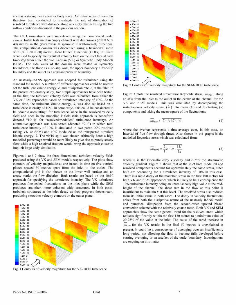
An unsteady-RANS approach was adopted for turbulence using the standard k-ε model. A number of different approaches could be used to set the turbulent kinetic energy, k, and dissipation rate, ε, at the inlet. In the present exploratory study, two simple approaches have been tested. In the first, the turbulent velocity field was calculated from either the VK or SEM approaches based on turbulence intensity of 10%. At the same time, the turbulent kinetic energy, k, was also set based on a turbulence intensity of 10%. In some ways, this could be considered to be “double accounting” for turbulence: once in the resolved velocity field and once in the modelled k field (this approach is henceforth denoted “10:10” for “resolved:modelled” turbulence intensity). An alternative approach was also tested (denoted “9:1”) in which total turbulence intensity of 10% is simulated in two parts: 90% resolved (using VK or SEM) and 10% modelled as the transported turbulent kinetic energy, k. The 90/10 split was chosen arbitrarily here: a high modelled percentage would be more likely to give rise to purely steady flow while a high resolved fraction would bring the approach closer to implicit large-eddy simulation. Figures 1 and 2 show the three-dimensional turbulent velocity fields produced using the VK and SEM models respectively. The plots show contours of velocity magnitude at one instant in time on five vertical planes spaced 50 metres apart from the inlet to the outlet. The computational grid is also shown on the lower wall surface and an arrow marks the flow direction. Both results are based on the 10:10 approach for specifying the turbulence intensity. The VK turbulence produces fine-scaled fluctuations on the inlet plane while the SEM produces smoother, more coherent eddy structures. In both cases, turbulent structures at the inlet decay as they progress downstream, producing smoother velocity contours on the outlet plane.

Fig. 1 Contours of velocity magnitude for the VK-10:10 turbulence

Fig. 2 Contours of velocity magnitude for the SEM-10:10 turbulence

Figure 3 plots the resolved streamwise Reynolds stress, resuu , along an axis from the inlet to the outlet in the centre of the channel for the VK and SEM models. This was calculated by decomposing the instantaneous velocity signal ( u~ ) into mean (U) and fluctuating (u) components and taking the mean-square of the fluctuations:

( ) ( )UuUuuu res −−= ~~ (1)

where the overbar represents a time-average over, in this case, an interval of five flow-through times. Also shown in the graphs is the modelled Reynolds stress which was calculated from:

xUkuu t ∂

∂−= ν232

mod (2)

where νt is the kinematic eddy viscosity and ∂U/∂x the streamwise velocity gradient. Figure 3 shows that at the inlet both modelled and resolved components account for approximately the same stress, since both are accounting for a turbulence intensity of 10% in this case. There is a rapid decay of the modelled stress in the first 100 metres for both VK and SEM approaches which is likely to be a consequence the 10% turbulence intensity being an unrealistically high value at the mid-height of the channel: the shear rate in the flow at this point is insufficient to maintain k at this level. The resolved stress also reduces from its initial value in both cases. The decay in velocity fluctuations arises from both the dissipative nature of the unsteady RANS model and numerical dissipation from the second-order upwind biased convection scheme with the relatively coarse mesh. Both VK and SEM approaches show the same general trend for the resolved stress which reduces significantly within the first 150 metres to a minimum value of 20-25% of the value at the inlet. The cause of the rapid increase in

resuu for the VK results in the final 50 metres is unexplained at present. It could be a consequence of averaging over an insufficiently long period, not allowing the flow to become fully-developed before starting averaging or an artefact of the outlet boundary. Investigations are ongoing on this matter.

Paper No. ISOPE-2008-__ Gant 7

0

0.02

0.04

0.06

0.08

0.1

0.12

0 20 40 60 80 100 120 140 160 180 200

Streamwise Distance

Stre

amw

ise

Rey

nold

s S

tress

VK Resolved VK Modelled SEM Resolved SEM Modelled

Fig. 3 Resolved and modelled streamwise Reynolds stress for VK and SEM, both using 10:10 turbulence intensity at the inlet.

0

0.02

0.04

0.06

0.08

0.1

0.12

0 20 40 60 80 100 120 140 160 180 200

Streamwise Distance

Stre

amw

ise

Rey

nold

s S

tress

VK Resolved VK Modelled SEM Resolved SEM Modelled

Fig. 4 Resolved and modelled streamwise Reynolds stress for VK and SEM, both using 9:1 turbulence intensity at the inlet.

The streamwise Reynolds stresses for the VK and SEM cases where at the inlet 90% of the turbulence energy was resolved and only 10% modelled are shown in Fig. 4. The difference between these results and the preceding 10:10 results is immediately apparent in the modelled stresses which start at a much lower (more realistic) value and are maintained at an almost constant level. Although the SEM resolved stress drops fairly sharply in the first 30 metres from the inlet, it thereafter remains relatively stable at a level above 40% of the inlet value. The VK resolved stress in contrast drops to value below 20% of the inlet value. The slightly less rapid decay of the SEM stress is probably due to the persistence of its more coherent eddy structures. The more stable behaviour of the SEM resolved stress is desirable, since it means that in later simulations where a tidal device is inserted into the channel the results should be less sensitive to the particular downstream position of the device.

HORIZONTAL AXIS DEVICE STUDY

Simulations have been performed to study the unsteady flow around a horizontal axis tidal current turbine using the Synthetic Eddy Method with 90% of the turbulence energy resolved and 10% modelled. The

swept area of the device was modelled in these simulations as a porous disc where the pressure drop through the disc was given by:

( )221 vkp ρ=∆ (3)

In the above expression k is the dimensionless resistance coefficient, ρ the density and v the velocity normal to the porous face. Taylor (1963) showed that the thrust coefficient for a flat sheet of porous material is given by:

( ) 2411 k

kCT+

= (4)

In order to simulate conditions where the turbine is operating at the Betz limit (i.e. the conditions where the theoretical maximum power coefficient is obtained, where CP = 0.59 and the corresponding thrust coefficient is CT = 0.89) the porosity of the disc in the CFD model has been set to k = 2.

Figures 5 and 6 compare the wake structure from simulations using a steady CFD approach and the unsteady SEM model. The results for the SEM are for just one instant in time. The extent of the wake region appears shorter in the unsteady results. There is also some motion of the wake in the unsteady simulations, which can be seen more clearly in animations (to be presented at the conference). At times, the wake is deflected closer to the floor, upwards or to the sides. To help understand the magnitude of these disturbances, Fig. 7 shows the velocity along the axis from the inlet to the outlet of the flow domain, passing through the centre of the actuator disc. The thick red line is the velocity predicted by a steady CFD simulation and the multiple coloured lines are the unsteady CFD results sampled at 500 instants in time over a period equivalent to five flow-through times (250 seconds). The plot indicates that, on average, the velocity recovers at a lower rate in the steady results. This is likely to be a consequence of the enhanced turbulent mixing in the unsteady case bringing in higher momentum fluid into the wake region. Overall, the results show similar trends to those of Sun et al. (2008), although the wake is somewhat longer here in terms of disc diameters. This is likely to be a consequence of the disc porosity, turbulence levels and Reynolds number being different in the two cases.

Paper No. ISOPE-2008-__ Gant 7

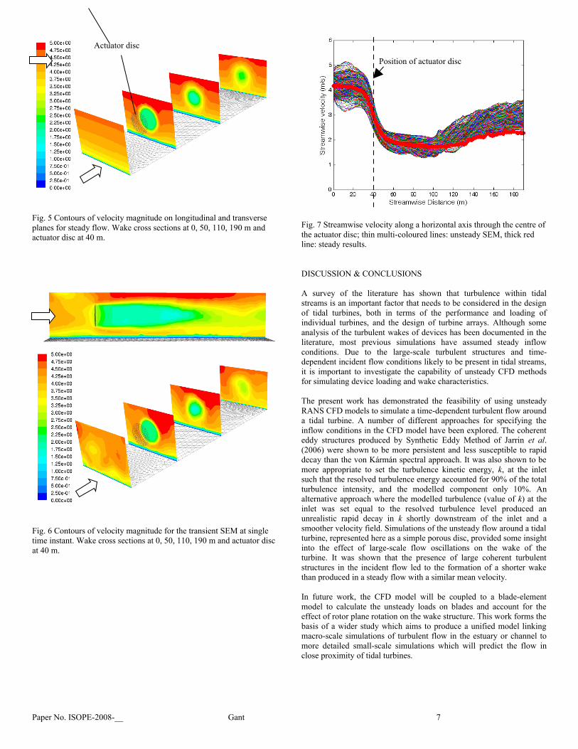
Fig. 5 Contours of velocity magnitude on longitudinal and transverse planes for steady flow. Wake cross sections at 0, 50, 110, 190 m and actuator disc at 40 m.

Fig. 6 Contours of velocity magnitude for the transient SEM at single time instant. Wake cross sections at 0, 50, 110, 190 m and actuator disc at 40 m.

Fig. 7 Streamwise velocity along a horizontal axis through the centre of the actuator disc; thin multi-coloured lines: unsteady SEM, thick red line: steady results.

DISCUSSION & CONCLUSIONS

A survey of the literature has shown that turbulence within tidal streams is an important factor that needs to be considered in the design of tidal turbines, both in terms of the performance and loading of individual turbines, and the design of turbine arrays. Although some analysis of the turbulent wakes of devices has been documented in the literature, most previous simulations have assumed steady inflow conditions. Due to the large-scale turbulent structures and time-dependent incident flow conditions likely to be present in tidal streams, it is important to investigate the capability of unsteady CFD methods for simulating device loading and wake characteristics.

The present work has demonstrated the feasibility of using unsteady RANS CFD models to simulate a time-dependent turbulent flow around a tidal turbine. A number of different approaches for specifying the inflow conditions in the CFD model have been explored. The coherent eddy structures produced by Synthetic Eddy Method of Jarrin et al. (2006) were shown to be more persistent and less susceptible to rapid decay than the von Kármán spectral approach. It was also shown to be more appropriate to set the turbulence kinetic energy, k, at the inlet such that the resolved turbulence energy accounted for 90% of the total turbulence intensity, and the modelled component only 10%. An alternative approach where the modelled turbulence (value of k) at the inlet was set equal to the resolved turbulence level produced an unrealistic rapid decay in k shortly downstream of the inlet and a smoother velocity field. Simulations of the unsteady flow around a tidal turbine, represented here as a simple porous disc, provided some insight into the effect of large-scale flow oscillations on the wake of the turbine. It was shown that the presence of large coherent turbulent structures in the incident flow led to the formation of a shorter wake than produced in a steady flow with a similar mean velocity.

In future work, the CFD model will be coupled to a blade-element model to calculate the unsteady loads on blades and account for the effect of rotor plane rotation on the wake structure. This work forms the basis of a wider study which aims to produce a unified model linking macro-scale simulations of turbulent flow in the estuary or channel to more detailed small-scale simulations which will predict the flow in close proximity of tidal turbines.

Paper No. ISOPE-2008-__ Gant 7

Actuator disc

Position of actuator disc

ACKNOWLEDGEMENTS

The authors would like to thank Dr. David Apsley, Dr. Antonio Filipponi, Prof. Peter Stansby, Prof. Dominique Laurence (all of the University of Manchester) for useful discussions. Special thanks also go to Nicholas Jarrin for providing the source code for the Synthetic Eddy Method. Funding provided by the NWDA Joule Centre through grant no. JSGP306/07 is appreciated.

REFERENCES

Batten, WMJ, Blunden, LS, Bahaj, AS, (2006). “CFD simulation of a small farm of horizontal axis marine current turbines”, Proceedings World Renewable Energy Congress (WREC) VIII, Florence, pp 19-25 Aug 2006.

Batten, WMJ, Bahaj, AS, Molland, AF and Chaplin, JR (2008). “The prediction of the hydrodynamic performance of marine current turbines”, Renewable Energy, (article in press).

BC Hydro (2002). Tidal Current Energy. Green Energy Study for British Columbia Phase 2: Mainland, Triton Consultants Ltd.

Carbon Trust (2005). Europe and global tidal stream resource assessment (Phase II), Black & Veatch (http://www.carbontrust.co.uk).

Carbon Trust (2006). Future Marine Energy Results of the Marine Energy Challenge: Cost competitiveness and growth of wave and tidal stream energy, (http://www.carbontrust.co.uk).

Couch, SJ, Jeffrey, HF and Bryden, IG (2006). “Proposed methodology for the performance testing of tidal current energy devices”, presented at Co-ordinated Action on Ocean Energy Workshop 4, Lisbon, 16-17th Nov 2006, (http://pmoes.ineti.pt).

Clarke, JA, Connor, G, Grant, AD and Johnstone, CM (2007). “Design and testing of a contra-rotating tidal current turbine”, Proc. IMechE Part A: J. Power and Energy, Vol 221, pp 171-179.

Dewey, R, Richmond, D and Garrett, C (2005). “Stratified tidal flow over a bump”, J. Phys. Oceanogr., Vol 35, pp 1911-1927.

DTI (2004). Atlas of UK marine renewable energy resources: Technical report. DTI Report No. R1106.

EPRI (2005). Tidal in Stream Energy Conversion (TISEC) devices: Survey and Characterisation. EPRI-TP-004 NA.

EPRI (2006). Methodology for Estimating Tidal Current Energy Resources and Power Production by Tidal In-Stream Energy Conversion (TISEC) Devices. EPRI-TP-001 NA Rev 2.

Garrad Hassan Ltd (2007). GH Tidal Bladed Theory Manual. Issue 17. Document No. 282/BR/009.

Gagnaire-Renou, E, Benoit, M, Buvat, C and Abonnel, C (2006). "Some lessons from tidal current and wave measurements at sea: Feedback of experience and analysis of measurements", presented at Co-ordinated Action on Ocean Energy Workshop 4, Lisbon, 16-17th

Nov 2006.Garrett, C and Cummins, P (2007). "The efficiency of a turbine in a

tidal channel". J. Fluid Mech. Vol 588, pp 243-251. doi:10.1017/S0022112007007781

Grant, HL, Stewart, RW and Moilliet, A (1961). “Turbulence spectra from a tidal channel”, J. Fluid Mech., Vol 12, pp 241-263.

IEC 61400-1:2005, Wind Turbines – Part 1: Design requirements (identical to BS EN 61400-1:2005).

Jarrin, N, Benhamadouche, S, Laurence, D and Prosser, R (2006). “A synthetic-eddy-method for generating inflow conditions for large-eddy simulations”, Int. J. Heat Fluid Flow, Vol 27, pp 585-593.

Jirka, GH (2001). “Large scale structures and mixing processes in shallow flows”, Journal of Hydraulics Research, Vol 39, pp 567–573.

Kawanisi, K and Yokosi, S (1994). “Mean and turbulence characteristics in a tidal river”, Estuarine, Coastal and Shelf Science, Vol 38, No 5, pp 447-469.

Lu, Y, Lueck, RG and Huang, D (2000). “Turbulence characteristics in a tidal channel”, J. Phys. Oceanogr., Vol 30, pp 855-867.

McCann, GN (2007). “Tidal current turbine fatigue loading sensitivity to waves and turbulence – a parametric study”, in Proc. 7th European Wave and Tidal Energy Conference, Porto, Portugal, 2007.

Myers LE, Bahaj AS (2005). “Simulated electrical power potential harnessed by marine current turbine arrays in the Alderney Race”, Renewable Energy, Vol 30, No 11, pp 1713–31.

Myers LE, Bahaj AS, (2005). "Wake Studies of a 1/30th scale Horizontal Axis Marine Current Turbine." in Proc. World Renewable Energy Congress (WREC) VII, Aberdeen, pp 1205–1210.

Norris, JV and Droniou, E (2007). "Update on EMEC activities, resource description, and characterisation of wave-induced velocities in a tidal flow", in Proc. 7th European Wave and Tidal Energy Conference, Porto, Portugal, 2007.

Shiono, K and West, JR (1987). “Turbulent perturbations of velocity in the Conwy estuary”, Estuarine, Coastal and Shelf Science, Vol 25, No 5, pp 533-553.

Sørensen, JN and Myken, A (1992). “Unsteady actuator disc model for horizontal axis wind turbines”, J. Wind Eng. Ind. Aerodyn., Vol 39, pp 139-149.

Sørensen, JN and Shen, WZ (2002). “Numerical modeling of wind turbine wakes”, J. Fluids Eng., Vol 124, pp 393-399.

Stansby, PK (2003). “A mixing length model for shallow turbulent wakes”, J. Fluid Mech., Vol 495, pp 369-384.

Sun, X, Chick, JP and Bryden, IG (2007). “Laboratory-scale simulation of energy extraction from tidal currents”, Renewable Energy, (article in press).

Taylor, GI (1963). “Air resistance of a flat plate of very porous material” and “The aerodynamics of porous sheets”, in The Scientific Papers of Sir Geoffrey Ingram Taylor, Vol. 3: Aerodynamics and the mechanics of projectiles and explosions, G.K. Batchelor, Editor. 1963, Cambridge University Press.

Veers, P (1988). Three-dimensional wind simulation, Sandia National Laboratories Report SAND-99-0152, Albuquerque, NM.

Paper No. ISOPE-2008-__ Gant 7