modelling and analysis for process control

Modelling andAnalysis for

Process Control4.1 ra INTRODUCTIONIn the previous chapter, solutions to fundamental dynamic models were developedusing analytical and numerical methods. The analytical integrating factor methodwas limited to sets of first-order linear differential equations that could be solvedsequentially. In this chapter, an additional analytical method is introduced thatexpands the types of models that can be analyzed. The methods introduced in thischapter are tailored to the analysis of process control systems and provide thefollowing capabilities:

1. The analytical solution of simultaneous linear differential equations with constant coefficients can be obtained using the Laplace transform method.

2. A control system can involve several processes and control calculations, whichmust be considered simultaneously. The overall behavior of a complex systemcan be modelled, considering only input and output variables, by the use oftransfer functions and block diagrams.

3. The behavior of systems to sine inputs is important in understanding how theinput frequency influences dynamic process performance. This behavior ismost easily determined using frequency response methods.

4. A very important aspect of a system's behavior is whether it achieves a steady-state value after a step input. If it does, the system is deemed to be stable; ifit does not, it is deemed unstable. Important control system analysis is basedon this behavior, and the methods in this chapter are applied to determine thestability of feedback control systems in Chapter 10.

98

CHAPTER 4Modelling andAnalysis for ProcessControl

All of the methods in this chapter are limited to linear or linearized systems ofordinary differential equations. The source of the process models can be the fundamental modelling presented in Chapter 3 or the empirical modelling presentedin Chapter 6.

The methods in this chapter provide alternative ways to achieve results thatcould, at least theoretically, be obtained for many systems using methods in Chapter 3. Therefore, the reader encountering this material for the first time might feelthat the methods are redundant and unnecessarily complex. However, the methods in this chapter have been found to provide the best and simplest means foranalyzing important characteristics of process control systems. The methods willbe introduced in this chapter and applied to several important examples, but theirpower will become more apparent as they are used in later chapters. The reader isencouraged to master the basics here to ease the understanding of future chapters.

4.2 n THE LAPLACE TRANSFORMThe Laplace transform provides the engineer with a powerful method for analyzingprocess control systems. It is introduced and applied for the analytical solution ofdifferential equations in this section; in later sections (and chapters), other applications are introduced for characterizing important behavior of dynamic systemswithout solving the differential equations for the entire dynamic response.

The Laplace transform is defined as follows:

£if(t)) = fis) = j°° me-xdt (4.1)

Before examples are presented, a few important properties and conventions arestated.

1. Only the behavior of the time-domain function for times equal to or greaterthan zero is considered. The value of the time-domain function is taken to bezero for t < 0.

2. A Laplace transform does not exist for all functions. Sufficient conditions forthe Laplace transform to exist are (i) the function fit) is piecewise continuousand (ii) the integral in equation (4.1) has a finite value; that is, the function /(/)does not increase with time faster than e~st decreases with time. Functions typically encountered in the study of process control are Laplace-transformableand are not checked. Further discussion of the existence of Laplace transformsis available (Boyce and Diprima, 1986).

3. The Laplace transform converts a function in the time domain to a functionin the "5-domain," in which s can take complex values. Recall that a complexnumber x can be expressed in Cartesian form as A + Bj or in polar form asRe*7" with

A = Re(;t) B = Im(jc) R = V' A2 + B2 <p = tan-1 (5) (4.2)

4. In this book, the Laplace transform of a function Tit) will be designated bythe argument s, as in Tis). The function and its transform will be designatedby the same symbol, which can be either a capital or a lowercase letter, andno overbar will be used for the transformed function. The function in thetime domain will be designated as the variable (as T) or with the time shownexplicitly [as 7X0], if needed for clarification.

5. The Laplace transform is a linear operator, because it satisfies the requirementsspecified in equation (3.36):

C[aFx (0 + bF2it)] = aC[Fx it)} + bC[F2it)] (4.3)

6. Tables of Laplace transforms are available, so the engineer does not have toapply equation (4.1) for many commonly occurring functions. Also, thesetables provide the inverse Laplace transform,

—iC~l[fis)) = fit) fort >0 (4.4)

Since the Laplace transform is defined only for single-valued functions, thetransform and its inverse are unique.

Before we proceed to the application of Laplace transforms to differentialequations, equation (4.1) is applied to a few functions that will be used in laterexamples. A more extensive list of Laplace transforms is given in Table 4.1.

99

The LaplaceTransform

ConstantFor/(0 = C,

C(C)Jo

Ce~st dt = - —es- S t C

s (4.5)

Step off Magnitude C at t = 0

For fit) = CUit) with 1/(0 =0 at t = 0+1 for t > 0+

CiCiUit))] = CC[Uit)] = CU e~st dt) = j(4.6)

Since the variable is assumed to have a zero value for time less than zero, theLaplace transforms for the constant and step are identical.

ExponentialFor fit) = e~at,

Cieat) -Lo o jat „-st -ea'e-sl dt = a — s

,-(.v-a)/|°°lo s — a (4.7)

100


TABLE 4.1

Laplace transformsN o . f { t )

12

3

4

5

6

7

8

9

10

1112

13

14

15

16

17

18

8, unit impulsei tt"

Uit), unit step or constant*n-\

in - 1)!

x

l + ^ - ^ e - "X

1 tn-le-'/Txn in - 1)!

1 + ( ^ - , ) e -

T'-V'/t, _ X2~a --/»

xx—aTi(r, -x2)

1 +T 2 - T i

sin i(ot)cos ioot)

e~a' cos (o>f)

e~a' sin icot)

, - ' / r i _ T 2 " a C i / W

72(T| - r2)

t 2 - r i

£e- sin[>/EI!r + 0t \ r

c j * : * + l j - - - / * ^\ - p l _ sia>re ,/r sin (art + cp)+\+C02X2 y / \+ (02X2

<f> = tan_I(—(*>x)

1 - 1VT=?

,-Wr sin 'VT^?■t + 4>

<j> = tan-1

/(0 =

' y / T ^

fi t - a ) t > a0 t < a

a, co, and t,- are real and distinct, 0 < £ < 1, n = integer

Ms)l1A\/sn

1TJ + 1

as + 17(t7+T)

1JxTTiy

as + 1(w +1)2

as + lsixs + l)2

flj + 1(riJ -I- l)(r2s + 1)

as + \sixxs + l)ix2s + 1)co/is2 + co2)s/is2 + co2)

s + ais + a)2

CO+ C02

(s + a)2 + C02

as + 1x2s2 + 2$xs + 1

CO

ixs + l)is2+co2)

1six2s2 + 2l-xs + \)

e-"sfis)

SineFor fit) = sin (cot),

r < x > r o o / j o t _ p - j ( o t \£(sin (at)) = / sin (a>t)e-st dt = / ( T j e~st

•oo /e-(s-ja))t _ e-(s+j<o)t

dt

-n_J_[e- (s -J

V )dt (4.8)

e-(s- j (o) t e - (s+ ja) t - I00 CO

co) (s + jco)]0 s2 + co2

PulseFor f(t) = C[UiO) - Uitp)] = C/tp for t = 0 to tp, and = 0 for t > tp, asgraphed in Figure 4.1,

f t p Q / . O OC(f(t)) = / -e-st dt + / Oe~st dt

J o h J t nC(\- e~stp) (4.9)

101


FIGURE 4.1

Pulse function.

An impulse function, which has zero width and total integral equal to C, is aspecial case of the pulse. Its Laplace transform can be determined by taking thelimit of equation (4.9) as tp -> 0 (and applying L'Hospital's rule) to give

C (1 - e~st")Y(s)\t.0 = lim

t P - + o t p s

= lim-c(-^)=cr » - > 0 s

(4.10)

Derivative off a FunctionTo apply Laplace transforms to the solution of differential equations, the Laplacetransform of derivatives must be evaluated.

(4.11)

This equation can be integrated by parts to give

c (r)= " i°° m(-s)e~5'dt+f{t)e~st= sf(s)-f(t)\t=0

The method can be extended to a derivative of any order by applying the integrationby parts several times to give

(4.12)

m-'f(s)

- (sn- /(OUo + s n-2 df(t)dt

in-1+ ...+ fit)

t=0 dtn~] J(4.13)

102n


In tegra l

By similar application of integration by parts the Laplace transform of an integralof a function can be shown to be

C (j* f(t') dA = j™ Qf f(t') dA e~st dt= f°° —fit) dt + \( f f(t) dt) —1 = -

J o s l \ J o ) s J / = o s

(4.14)f(s)

'AO

■ b '■

do

Different ia l Equat ions

One of the main applications for Laplace transforms is in the analytical solutionof ordinary differential equations. The key aspect of Laplace transforms in thisapplication is demonstrated in equation (4.13), which shows that the transform ofa derivative is an algebraic term. Thus, a differential equation is transformed into analgebraic equation, which can be easily solved using rules of algebra. The challengeis to determine the inverse Laplace transform to achieve an analytical solution inthe time domain. In some cases, determining the inverse transform can be complexor impossible; however, methods shown in this section provide a general approachfor many systems of interest in process control. First, the solutions of a few simplemodels involving differential equations, some already formulated in Chapter 3, arepresented.EXAMPLE 4.1.The continuous stirred-tank mixing model formulated in Example 3.1 is solvedhere. The fundamental model in deviation variables is

dCV - A = F ( C A Q - C A ) ( 4 . 1 5 )The Laplace transform is taken of each term in the model:

V [sC'Ais) - C'Ait)\tJ = F [C'AQis) - C'Ais)] (4.16)The initial value of the tank concentration, expressed as a deviation variable, iszero, and the deviation of the inlet concentration is constant at the step value fort > 0; that is, CA0(O = ACAoA- Substituting these values and rearranging equation(4.16) gives

CA(0 =ACAO 1 with x = — = 24.7 min (4.17)S X s + 1

The inverse transform of the expression in equation (4.17) can be determined fromentry 5 of Table 4.1 to give the same expression as derived in Example 3.1.

CA(0 = ACAO(l-<r'/r) (4.18)

'AO

CD' A l

bCO

'A2

EXAMPLE 4.2.The model for the two chemical reactors in Example 3.3 is considered here, andthe time-domain response to a step change is to be determined. The linear component material balances derived in Example 3.3 are repeated below in deviationvariables.

Vi dtAl = F iC ' -C ' ) -VkC '' A l (3.24)

103V 2 — A - = F ( C A 1 - C ^ ) - V k C A 2 ( 3 . 2 5 ) h m w h i b w i i — Ia i T h e L a p l a c e

The Laplace transforms of the component material balances in deviation variables, Transformnoting that the initial conditions are zero, are

sVC'Alis) = F(C'AOis) - C'AXis)) - VkC'Alis) (4.19)sVC'^is) = F (CAlis) - C'A2is)) - VkC'^is) (4.20)

These equations can be combined into one equation by eliminating C'A]is) fromthe second equation. First, solve for C'AXis) in equation (4.19):

KF + Vk)^C » = „ + 1 C a o ( 4 - 2 1 )

This expression can be substituted into equation (4.20) along with the input stepdisturbance, CAOis) = ACA0/s, to give

KpACApsixs + l)2C « W = ^ = ( 4 - 2 2 )

V m o l ewith x = -——- = 8.25 min ACA0 = 0.925 —r2 m o l e

K ^ ( - d v k ) = 0 m C „ . - 0 A U mJThe inverse transform can be determined from entry 8 of Table 4.1 to give theresulting time-domain expression for the concentration in the second reactor.

c^4V,[ i - ( . + i )^ ] (423)CA2(0 = 0.414 + 0.414(1 - <?-'/8-25) - 0.050f<r'/8-25

This is the same result as obtained in Example 3.3.

Time Translation or Dead TimeThe Laplace transform for a dead time of 0 units of time is

• o o / * o o/ • o o / » o o

C[fit -9))= fit - e)e~st dt = e~9s / /(/ - 0)*-*('-0) dit - 9)J o J o ( 4 2 4 )/•OO

= e~6s / fit')e~st' dt' = e~6sfis)Jo

When changing variables from it -9) to t', the lower bound of the integral remainedat 0 (did not change to t'-9), because the function is defined /(/) = Oforf < Oforthe Laplace transform. The expression in equation (4.31) is used often in processmodelling to represent behavior in which the output variable does not respondimmediately to a change in the input variable; this condition is often referred to asdead time.

104


0 LengthFIGURE 4.2Schematic of plug flow process.

•a"8■8 0.5E$« o

^* -0.5

i r i r i r

\—e—\

0 1 2 3 4 5 6 7Time

FIGURE 4.3Input and output for dead time (0) of one time unit.

time1 1 1 T 1 1 1 i i

1 0.5"O / \/ \2 / \ / — S ^O 0is V ^ y " ^>< i i i i i i i i i

10

EXAMPLE 4.3.The dynamic behavior of turbulent fluid flow in a pipe approximates plug flow, withthe fluid properties like concentration and temperature progressing down the pipeas a front. The dead time is 6 - L/v, i.e., the length divided by the fluid velocity.The inlet concentration to the pipe in Figure 4.2 is X, and the outlet concentrationis Y. For ideal plug flow,

Y i t ) = X i t - 6 ) ( 4 . 2 5 )The Laplace transform of this model can be evaluated using the results in equation(4.24) to give

Y i s ) = X i s ) e ~ 9 s ( 4 . 2 6 )The effect of a dead time for an arbitrary input concentration is shown in Figure 4.3.

Final Value Theorem

The final condition of the transient can be determined by applying the expressionfor the derivative of a function, equations (4.11) and (4.12), and taking the limitas s -» 0. ,0° dfit)

limu: dt -stdt\ = \\m[sf(s)-f(t)]t=0Changing the order of the limit and the integral gives

,0° dfit)/Jo

. dt = \im\sfis) - fit)]a t 5 - > o

/(oo) - /(OU = HmW(s) - fit)]s->0

/(oo) = lim sfis)s-*0

t=0

t = 0

(4.27)

(4.28)

Equation (4.28) provides an easy manner for finding the final value of a variable;however, one should recognize that a simpler method would be to formulate andsolve the steady-state model directly. The final value theorem finds use because thedynamic models are required for process control, and the final value can be easilydetermined from the Laplace transform without further modelling effort. Also, itis important to recall that the final value is exact only for a truly linear process andis approximate when based on a linearized model of a nonlinear process.

EXAMPLE 4.4.Find the final value of the reactor concentration, expressed as a deviation fromthe initial value, for the CSTRs in Example 4.2. The Laplace transform for theconcentration in response to a step in the inlet concentration is given in equation(4.22). The final value theorem can be applied to give

\\ms(CA2is)) = lim ( js - * 0 s - * 0 \ACAp Kp

s ixs + \) ) = KPACA0 = (7F7™) ACao (4-29)Note that this is the final value, which gives no information about the trajectory tothe final value.

The engineer must recognize a limitation when applying the final value theorem. The foregoing derivation is not valid for a Laplace transform fis) that isnot continuous for all values of s > 0 (Churchill, 1972). If the transform has adiscontinuity for s > 0, the time function fit) does not reach a final steady-statevalue, as will be demonstrated in the discussion of partial fractions. Therefore, thefinal value theorem cannot be applied to unstable systems.EXAMPLE 4.5.Find the final value for the following system.

KYis) = (AX) sixs — 1)

with r > 0

This transfer function has a discontinuity at s = 1/r > 0; therefore, the final valuetheorem does not apply. The analytical expression for Yit) is

Yit) = iAX)Ki\ -e"x) (4.30)The value of Yit) approaches negative infinity as time increases; this is not equalto the incorrect result from applying the final value theorem to the transfer function-KiAX).

Init ial Value TheoremThe initial value of a variable can be determined using the initial value theorem.The derivation begins in the same manner as the final value theorem, except that thelimit is taken as s -> co. Again, the order of the limit and integration is changed,resulting in the following equation:

105


'AO

doU-

' A l

db 'A2

Initial value theorem /(OUo = lim sf(s) (4.31)

106

CHAPTER4Modelling andAnalysis for ProcessControl

-Ao- W

do ' A l

do-A2

EXAMPLE 4.6.The model for the two series CSTR chemical reactors in Examples 3.3 and 4.2 isconsidered in this example with the alteration that the volumes of the two reactorsare not the same volume, Vi = 1.4 and V2 = 0.70 m3. Determine the time-domainresponse.

The Laplace transforms of the two linear component material balance modelsin deviation variables are

sViCM(s) = F[C'AOis) - CM(s)] - VxkCAlis) (4.32)

sViC^is) = F[C'Mis) - CA2is)] - V2kC'A2is) (4.33)These equations can be combined into one equation by solving for CA1 is) in equation (4.32) and substituting this into equation (4.33). Also, the input step disturbance can be substituted, C'Mis) = ACA0/s, to give

K p C A o ( s ) K p A C A oCWO = (xxs + \)ix2s + 1) sixxs + \)ix2s + 1) (4.34)

with

T i =V,

T 2 =v2 K,

\F + Vxk)\F + V2k)F + Vxk F+V2k "y \F + Vxk) \F + V2k tThe inverse Laplace transform can be evaluated using entry 10 in Table 4.1 (witha — 0) to determine the time-domain behavior of the concentration in the secondreactor.

CUt) = KPACA0 1 + ,-</*! - -^—e-<lAT 2 - T i J

(4.35)r 2 - x x - -This response is a smooth j-shaped curve, but it has different values at every timefrom the original CSTR system.

EXAMPLE 4.7.Using Laplace transforms, determine the response of the level in the draining tank(Example 3.6) to two different changes to the inlet flow, (a) a step and (b) animpulse.Data. Cross-section area A = 7 m2, initial flows in and out, = 100 m3/min, initiallevel = 7 m, kFX = 37.8 (m3/h)/(m-°-5). The model for the draining tank level isbased on an overall material balance of liquid in the tank depending on the flowin (Fo)andout(Fi).

dLpA— - pF0 - pFx (4.36)

The tank cross-sectional area is A. The flow out depends on the level in the tankthrough a nonlinear relationship, and after linearization, the level model is

t 1 T + l ' = k p f ° < 4 - 3 7 )with x = A/i0.5kF, L;0-5) = 0.98 h

Kp = \/i0.5kFXL;05) = 0.14 m/(m3/h)The Laplace transform of equation (4.37) can be taken to give

KrL'is) = xs + \ Fiis) (4.38)

(a) For a step change in the inlet flow rate, Fq(s) = AF0/(O; this expression canbe substituted into equation (4.38), and the inverse Laplace transform can beevaluated using entry 5 in Table 4.1. The resulting expression for the draininglevel response to a step flow change is

L ' i t ) = K p A F Q i \ - e - ' / x ) ( 4 . 3 9 )As.already determined in Example 3.6, the level dynamic response beginsat its initial condition and increases in a "first-order" manner to its final value,which it reaches after about four time constants.

(b) An impulse is a change that has a finite integral but zero duration! Beforeevaluating the impulse response, we should understand how this could occurphysically. For the level process, an impulse can be approximated by introducing additional liquid very rapidly: one method for implementing an impulsein this system would be to empty a bucket of liquid into the tank very fast. Theintegral of the impulse is evaluated as

/ F < J ( 0 d t = M m 3 ( 4 . 4 0 )

The Laplace transform of the impulse, F^is) = M, can be introduced intoequation (4.38) to give

xs + \The inverse Laplace transform can be evaluated using entry 4 in Table 4.1,which gives [substituting the definition of the gain Kp = x/iA)] the followingresult:

L ' i t ) = h E e - t h = M e _ t l x ( 4 4 1 )x AThe dynamic response of the draining tank level to an impulse of M = 20 m3 isshown in Figure 4.4. For the parameters in the example, the levels calculatedusing the nonlinear and linearized models are nearly identical. The level immediately increases in response to the addition of liquid. Since the inlet flowreturns to its initial value after the impulse, the level slowly returns to its initialvalue.

Part ia l Fract ionsThe Laplace transform method for solving differential equations could be limitedby the entries in Table 4.1, and with so few entries, it would seem that most modelscould not be solved. However, many complex Laplace transforms can be expressedas a linear combination of a few simple transforms through the use of partial fractionexpansion. Once the Laplace transform can be expressed as a sum of simplerelements, each can be inverted individually using the entries in Table 4.1, thusgreatly increasing the number of equations that can be solved. More importantly,the application of partial fractions provides very useful generalizations about theforms of solutions to a wide range of differential equation models, and thesegeneralizations enable us to establish important characteristics about a system'stime-domain behavior without determining the complete transient solution. Thepartial fractions method is summarized here and presented in detail in Appendix H.

108


10

9.5

1 1 1 r i i i i i

9 \ -

8.5 - \ ^ -

8 _ > v -

E£ 7 . 53

- ^ \ ^ ^ -7

6.5 — -

6 - -

5.5 -

1 1 1 1 1 1 _ l 1 J

0 0 . 5

FIGURE 4.4

1 . 5 2 2 . 5 3Time (h)

3.5 4.5

Response of the draining tank level in Example 4.7 to an impulse inthe flow in (F0) at time t = 0.50 h.

The reader may have noticed that nearly all Laplace transforms encountered tothis point are ratios of polynomials in the Laplace variable s. The partial fractionsmethod can be used to express a ratio of polynomials as a sum of simpler terms.For example, if the roots of the denominator are distinct, a ratio of higher-ordernumerator and denominator polynomials can be expressed as the sum of terms, allof which have constant numerators and first-order denominators, as given below.

Yis) = N(s)/D(s) = Ci/is - «i) + C2/(s - a2) + (4.42)

with Y(s) = Laplace transform of the output variableN(s) = numerator polynomial in s of order mD(s) = denominator polynomial in s of order n (n > m), termed the

characteristic polynomialC\ — constants evaluated for each problema,- = distinct roots of D(s) = 0

The inverse Laplace transform of the original term Y(s), which might not appearin a table of Laplace transforms, is the sum of the inverses of the simpler termsCi/(s — a,), which appear as entry 4 in Table 4.1. This method is extended torepeated and complex denominator roots in Appendix H, where it is applied todetermining the inverse of a complicated Laplace transform. However, the majorusefulness for partial fractions is in proving how several key aspects of a variable'sbehavior can be determined directly from the Laplace transform without solvingfor the inverse.

One key finding is summarized here, and another will be developed in Section4.5 on frequency response. For any differential equation which can be arranged

into the form of equation (4.42), the inverse Laplace transform will be of the form 109

Yit) = Ax** + --- + (Bl+B2t + -' •)«"'' + • ■ ■ +(4.43)

Number ofzero roots Terms in so lu t ion Is the system stab le?Only one Axe° = Ax — constant YesTwo (or more) (Bx + B2t)e° = (Bx + B2t) No, this term increases in

magnitude without limit

2. Damping. The nature of the roots of the characteristic polynomial determineswhether the dynamic response will experience periodic behavior for nonperi-odic inputs; complex roots of D(s) lead to periodic (underdamped) behavior,and real roots lead to nonperiodic (overdamped) behavior.

These two results enable the engineer to determine key features of the dynamicperformance of systems without evaluating the complete dynamic transient viainverse Laplace transform. The simplification is enormous!

Certainly, a process would be easier to operate when it is stable so that vari ablesrapidly approach constant values and no variables tend to increase or decreasewithout limit (based on a linearized model). Also, while oscillations are not usuallycompletely avoided, oscillations of large magnitude are generally undesirable.Thus, the nature of the roots of the characteristic polynomial and how processdesign and control algorithms affect these roots are important factors in designinggood processes and controls. These issues will be investigated thoroughly in PartIII on feedback control by evaluating the roots of the characteristic polynomial, andthe partial fraction method provides the mathematical foundation for this importantanalysis.

The Laplace[ C , C O S ( c o t ) + C 2 S i n ( c o t ) ] e a « ( + • • • T r a n s f o r m

This equation includes distinct (a\), repeated real (ap), and complex roots (aq), notall of which may appear in a specific solution, in which case some of the constants(A, B, or C) will be zero. Two important conclusions can be drawn:

1. Stability. The real parts of the roots of the characteristic polynomial, Dis),determine the exponents (a's) in the solution. These exponents determinewhether the function approaches a constant value after a long time. For example, when all real parts of the roots, i.e., all Re(a,), are negative, all terms onthe right of equation (4.43) approach a constant value after an initial transient;a system which tends toward a constant final value is termed stable. If anyRe(a,) is greater than zero, the function Yit) will increase (or decrease) in anunbounded manner as time increases; this is termed unstable.

We must look carefully at the case of roots with a value of zero. If onedistinct root has a value of zero, the system is stable, while if repeated rootshave values of zero, the system is unstable. This result is summarized in thefollowing.

110


'AO

CD'Al

do 'A2

EXAMPLE 4.8.Determine whether the concentration in the second reactor in Example 4.6 is stableand underdamped without solving for the concentration.

The roots of the denominator of the Laplace transform can be evaluated todetermine these key aspects of the dynamic behavior. The Laplace transform isrepeated below.

C'(s) = KPACAQs(xxs + l)(x2s + 1) (4.44)

The roots of the denominator, which are the exponents, are -1/ti, -1/t2, and 0.0.Since both nonzero time constants are positive, the roots are less than zero; also,only one zero root exists. Therefore, the concentration reaches a constant valueand is stable. Also, since the roots are real, the concentration is overdamped. Naturally, these conclusions are consistent with the equation defining the time-varyingconcentration derived in Example 4.5; however, the conclusions were reachedhere with minimal effort and can be determined for more complex Laplace transforms that do not appear in Table 4.1.

4.3 m INPUT-OUTPUT MODELS AND TRANSFER FUNCTIONSIn some cases the values for all dependent process variables need to be determinedto meet modelling goals, and the fundamental models used to this point in thebook, which provide expressions for all variables, can be used in these cases.For example, the model for two series CSTRs in Example 3.3 yields expressionsfor the concentrations in both reactors. Some models are not unduly complex;however, detailed models can involve a large number of equations. For example,a distillation tower with 40 trays and 10 components would require over 400differential equations.

A fundamental model solving for all dependent variables is often not requiredfor process control, because the control system is principally involved with allinput variables but only one or a few output variables. Thus, we need a methodfor "compressing" the model, which can be achieved by first grouping variablesinto three categories: input (causes), output (effects), and intermediate. For lineardynamic models used in process control, it is possible to eliminate intermediatevariables analytically to yield an input-output model, so that intermediate variablesare considered in the model even though they are not explicitly calculated. Thus,no further assumptions or simplifications are involved in input-output modellingof linear systems.

Examples of this approach have already been encountered in this chapter.For example, the basic model for two series CSTRs in Example 4.6 includedequations for the concentrations in both reactors, equations (4.32) and (4.33).After the Laplace transforms are taken and the equations are combined into oneequation, the model in equation (4.34) involves only the input, C'AOis), and theoutput, C'A2is). The intermediate variable, C'Alis), was eliminated, although alleffects of the first reactor are represented in the model.

A very common manner for presenting input-output models, which findsconsiderable application in process control, is the transfer function. The trans-

fer function is a model based on Laplace transforms with special assumptions,as follows.

I l l

The transfer function of a system is defined as the Laplace transform of the outputvariable, 7(0, divided by the Laplace transform of the input variable, Xit), with allinitial conditions equal to zero.

Transfer function = Gis) = Yjs)Xis) (4.45)

The assumptions of Y (0) = 0 and X(0) = 0 are easily achieved by expressing thevariables in the transfer function as deviations from the initial conditions. Thus, alltransfer functions involve variables that are expressed as deviations from an initialsteady state. All derivatives are zero if the initial conditions are at steady state.(Systems having all zero initial conditions are sometimes referred to as "relaxed.")These zero initial conditions are assumed for all systems represented by transferfunctions used in this book; therefore, the prime symbol"'" for deviation variablesis redundant and is not used here when dealing with transfer functions. Transferfunctions will be represented by Gis), with subscripts to denote the particularinput-output relationship when more than one input-output relationship exists.Before proceeding with further discussion of transfer functions, a few examplesare given.

EXAMPLE 4.9.Derive the transfer functions for the systems in Examples 4.1 and 4.2. The Laplacetransform of the model in Example 4.1 is in equation (4.16). This can be rearrangedto give the transfer function for this system:

Example 4.1: CA(0 1xs + 1

Vwith x = —F (4.46)CaoOOThe Laplace transform for the model in Example 4.2 can be rearranged to givethe transfer function for this system:

Example 4.2:KrCA2js) =

CAOis) ixs +1)2 (4.47)

with x =

Kp =

F + V kF

\F + Vk)The models from the previous examples could be used to form transfer functions,because they were in terms of deviation variables with zero initial conditions.

Note that the transfer function relates one output to one input variable. Ifmore than one input or output exists, an individual transfer function is defined foreach input-output relationship. Since the transfer function is a linear operator (as

112


'AO

Udo

V C A

a result of the zero initial conditions), the effects of several inputs can be summedto determine the net effect on the output.

EXAMPLE 4.10.Derive the transfer functions for the single CSTR with the first-order reaction inExample 3.2 for changes in the inlet concentration and the feed flow rate.

The two linear models for each input change can be determined by assumingthat all other inputs are constant. The basic model was derived in Example 3.2 andis repeated below.

V^£ = FiCM-CA)-VkCAat (4.48)

To determine whether the model is linear or not, the constant values are substituted(noting that the flow and inlet concentrations are now variables) to give

<2.1)^r = F(Ca° - Ca> - (2.D(0.040)CAdtThe model is nonlinear because of the products of flow times concentrations.Two linearized models can be derived from equation (4.48), one for each input(assuming the other input constant), to give

tca-dC\dt + CA = KCACA0

t f ^+C 'a = K fF '

withT«=Grrw) *«=GnW(4'49)

Taking the Laplace transforms and rearranging yields the two transfer functions,one for each input.

CAjs)CaoCO

= GcAis) = &CA

tCAs +1

£^1 = Gf(s) = - -F ( s ) F V x F s + 1

(4.51)

(4.52)

These models and transfer functions give the behavior of the system output forindividual changes in each input. If both inputs change, the overall effect is approximately the sum of the two individual effects. (If the process were truly linear,the total effect would be exactly the sum of the two individual effects.) Readersmay want to return to Section 3.4 to refresh their memory on linearization.

The transfer function clearly shows some important properties of the systembriefly discussed below.

Orde rThe order of the system is the highest derivative of the output variable in thedefining differential equation, when expressed as a combination of all individual equations. For transfer functions of physical systems, the order can be easilydetermined to be the highest power of s in the denominator.

PoleA pole is defined as a root of the denominator of the transfer function; thus, it isthe same as a root of the characteristic polynomial. Important information on thedynamic behavior of the system can be obtained by analyzing the poles, such as

1. The stability of the system2. The potential for periodic transients, as shown clearly in equation (4.43)

The analysis of poles is an important topic in Part III on feedback systems, sincefeedback control affects the poles.

ZeroA zero is a root of the numerator of the transfer function. Zeros do not influencethe exponents (Re(a)), but they influence the constants in equation (4.43). Thiscan most easily be seen by considering a system with n distinct poles subject to animpulse input of unity. The expression for the output, since the Laplace transformof the unity input impulse is 1, is

N ( s ) M i ( s )Y(s) = G(s)X(s) = G(s) = for i = 1, n (4.53)D(s) s — a,-For a system with no zeros, the numerator would be equal to a constant, N(s) = K,and the constant associated with each root is

With no zeros " U(*)/,«, (4.54)

Dt (s) is the denominator, with (s — a,) factored out. For a system with one or morezeros, the constant associated with each root is

With zeros 1 V Aco/,=_ff, (4.55)

Thus, the numerator changes the weight placed on the various exponential terms.This demonstrates that the numerator of the transfer function cannot affect thestability of the system modelled by the transfer function, but it can have a stronginfluence on the trajectory followed by variables from their initial to final values.A simple, but less general, example to demonstrate the effect of numerator zerosis seen in the following transfer function.

G ( s ) = ^ i i _ 1 ( 4 . 5 6 )w (3s + 1)(2.5j + 1) 2.5^ + 1The numerator zero cancelled one of the poles, with the result that the second-ordersystem behaves like a first-order system. Important examples of how zeros occurin chemical processes and how they influence dynamic behavior are presented inthe next chapter, Section 5.4.

Order of Numerator and Denominator

Physical systems conform to a specific limitation between the orders of the numerator and denominator; that is, the order of the denominator must be larger than

114


the order of the numerator. This limitation results from the observation that realphysical systems do not contain pure differentiation, as would be required for asystem with a numerator order greater than the denominator order.

Causa l i t yAs discussed in Chapter 1 in the introduction of feedback control, the "direction" ofthe cause-effect relationship is essential to control system design. This direction ispresented in the transfer function by identifying the variable in the denominator asan input (cause) and in the numerator as an output (effect). In designing feedbackcontrol strategies, the variable chosen to be adjusted must be an input, and themeasured controlled variable used for determining the adjustment must be anoutput. When the physical system is causal, the order of the denominator is greaterthan that of the numerator, and the value of the transfer function as s -> co isequal to 0. Such a transfer function is referred to as strictly proper.

Also, the current value of a system output variable can depend on past valuesof the output and inputs, but it cannot depend on future values of any variable.Therefore, the transfer function must not have prediction terms. By equation (4.24),the transfer function may not contain a term eds, which is a translation into the future(that cannot be eliminated by rearranging the transfer function). Such models arereferred to as noncausal or not physically realizable, because they cannot representa real physical system.

'AO

-W-do ' A l

■Wdb 'A2

Steady-State GainThe steady-state gain is the steady-state value of A Y/ AX for all systems whoseoutputs attain steady state after an input perturbation AX. The steady-state gain isnormally represented by K, often with a subscript, and can be evaluated by settings = 0 in the (stable) transfer function. This is exact for linear systems and givesthe linearized approximation for nonlinear systems.

EXAMPLE 4.11.Determine the stability and damping of the outlet concentration leaving the last oftwo isothermal CSTRs in Examples 4.2 and 4.9.

The transfer function for this system was derived in Example 4.9 and is repeated below.

CA2(Q = G ( ) _ KPC a o C O ( w + D 2 (4.57)

The order of the system is the highest power of s in the denominator, 2. This indicates that the process can be modelled using two ordinary differential equations.The poles are the roots of the polynomial in the denominator; they are repeatedroots, a = -1/t = -1/8.25 min-1 = -0.1212 min"1. The dynamic behavior is non-periodic (overdamped), because the poles are real and not complex. Also, thepoles are negative, indicating that the process is stable.

For a stable process, the steady-state gain can be determined by settings = 0 in the transfer function.

Steady-state gain: iGis))s=0 = KpAlso, the final value of the reactant concentration in the second reactor can be

e v a l u a t e d u s i n g t h e fi n a l v a l u e t h e o r e m . 1 1 5

— ) ( T T T T ) = K ' A C a o B l o c k D i a g r a m s

In a specific situation the behavior of an output variable, from time 0 to completion of the response, depends on its initial conditions, input forcing, and transferfunction (input-output) model. However, some very important properties of linear dynamic systems depend only on the transfer function, because the propertiesare independent of initial conditions and type of (bounded) forcing functions. Forexample, the stability of the system was shown in the previous section to be determined completely by the roots of the characteristic polynomial. The primary application of transfer functions is in the analysis of such properties of linear dynamicsystems, and they are applied extensively throughout the remainder of the book.

4.4 0 BLOCK DIAGRAMSThe transfer function introduced in the previous section describes the behavior ofthe individual input-output system on which it is based. Often, several differentindividual systems are combined, and the behavior of the combined system is tobe determined. For example, a control system could involve individual systemsfor a reactor, a distillation tower, a sensor, a valve, and a control algorithm. Theoverall model could be derived by writing all equations in a large set, taking theLaplace transforms, and combining into one transfer function. Another approachretains the distinct transfer functions of the individual systems and combines thesetransfer functions into an overall model. This second approach is usually preferredbecause

1. It retains individual systems, thereby simplifying model changes (e.g., a different sensor model).

2. It provides a helpful visual representation of the cause-effect relationships inthe overall system.

3. It gives insight into how different components of the system influence theoverall behavior (e.g., stability).

The block diagram provides the method for combining individual transferfunctions into an overall transfer function. The three allowable manipulations ina block diagram are shown in Figure 4.5a through c. The first is the transformof an input variable to an output variable using the transfer function; this is justa schematic representation of the relationship introduced in equation (4.45) anddiscussed in the previous section. The second is the sum (or difference) of twovariables; the third is splitting a variable for use in more than one relationship.These three manipulations can be used in any sequence for combining individualmodels. A more comprehensive set of rules based on these three can be developed(Distephano et al., 1976), but these three are usually adequate.

To clarify, a few illegal manipulations, which are sometimes mistakenly used,are shown in Figure A.5d through /. The first two are not allowed because the

116


Allowed

Yis)

X3is)

X2(s)Xxis) + X2is) = X3is)

i c ) i * - X 2 i s )

Xxis)—|

id)

Not Allowed

-<MW"

X2is)—* G{s) — ^ Y i s )

ie)* ( * )—•* Gis) —+- Yxis)

—▶ Y2is)

-+■ X3is)

Xxis) = X2is) = X3is)FIGURE 4.5

if) Xxis)

X2is)

X3is)

[Xlis)][X2is)]=X3is)

Summary of block diagram algebra: ia-c) allowed; id-f) notallowed.

'AO

- Udo ' A l

bdo 'A2

transfer function is defined for a single input and output, and the third is notallowed because the block diagram is limited to linear operations.

The block diagram can be prepared based on linearized models (transfer functions) of individual units and the knowledge of their interconnections. Then aninput-output model can be derived through the application of block diagram algebra, which uses the three operations in Figure 4.5a through c. The model reductionsteps normally followed are

1. Define the input and output variables desired for the overall transfer function.2. Express the output variable as a function of all variables directly affecting it

in the block diagram. This amounts to working in the direction opposite to thecause-effect relationships (arrows) in the diagram.

3. Eliminate intermediate variables by this procedure until only the output andone or more inputs appear in the equation. This is the input-output equationfor the system.

4. If a transfer function is desired, set all but one input to zero in the equationfrom step 3 and solve for the output divided by the single remaining input.This step may be repeated to form a transfer function for each input.

The following examples demonstrate the principles of block diagrams, andmany additional applications will be presented in later chapters.EXAMPLE 4.12.Draw the block diagram for the two chemical reactors in Example 4.2, and combinethem into one overall block diagram and transfer function for the input CA0 andthe output CA2. The individual transfer functions are given below and shown inFigure 4.6a.

ia)GAQis)

FCAXis)

FF+Vk F+Vk GA2is)

^-TS+ 1 TS+ 1

117

Block Diagrams

ib)CA0is)

F 2CA2is)

. F + V k

[TS + I]2

FIGURE 4.6Block diagrams for Example 4.12.

Gxis) =

G2is) =

CMjs)CAOis)CA2is)

K>xs + \

K2

with r =

with x =

F + VkV

K, =

K j =

F + VkF

(4.58)

(4.59)C a i ( j ) x s + \ F + V k ' " ' F + V kBlock diagram manipulations can be performed to develop the overall input

output relationship for the system.CA2 = G2is) CaiCs) = G2is) [Giis) CAOis)] = G2is) Gxis)CAOis)

KXK2 ;CAOis)(4.60)

ixs + l)2This can be rearranged to give the transfer function and the block diagram inFigure 4.6b.

Ca2(*) = = KXK2CAOis) {S) ixs +1)2 (4.61)

EXAMPLE 4.13.Derive the overall transfer functions for the systems in Figure 4.7. The system inpart (a) is a series of transfer functions, for which the overall transfer function isthe product of the individual transfer functions.

X„is) = Gnis) Xn-iis) = GM G„_,(j) X._2(j)= G„is) Ga-iis) Gn.2is) -Giis) Xois)

Xnjs)Xois)

(4.62)

= Y\G'i = i

The system in part (b) involves a parallel structure of transfer functions, andthe overall transfer function can be derived as

X3is) = X, is) + X2is) = G, is) X0is) + G2is) XQis)X3is)

(4.63)

Xois)= Gxis) + G2is)

118


(a)X0is)

Gxis)Xj(i)

G2X2is)

G3is) Gnis)Xnis)

(b)

Xois)-

1 *■ Gxis)Xxis)

*•<C

▶» G2is)X2is)

»•

<§>—+~X3is)

(c)Xxis)

X0is)-+-®—*- Gxis)X2is)

X3is) G2is) ^

FIGURE 4.7Three common block diagram structures considered in Example 4.13.

The system in part (c) involves a recycle structure of transfer functions, andthe overall transfer function can be derived as

X2is) = Gxis) Xxis) = Gxis) [X0is) + X3is)] = Gxis) [Xois) + G2is)X2is)]Gxis)X2js) =

Xois) \-Gxis)G2is)(4.64)

Examples of processes that can be represented by these structures, alongwith the effects of the structures on dynamic behavior, will be presented in the nextchapter.

It is perhaps worth noting that the block diagram is entirely equivalent to andprovides no fundamental advantage over algebraic solution of the system's linearalgebraic equations (in the s domain). Either algebraic or block diagram manipulations for eliminating intermediate variables to give the input-output relationshipwill result in the same overall transfer function. However, as demonstrated by theexamples, the block diagram manipulations are easily performed.

Two further features of block diagrams militate for their extensive use. Thefirst is the helpful visual representation of the integrated system provided by theblock diagram. For example, the block diagram in Figure 4.7c clearly indicates arecycle in the system, a characteristic that might be overlooked when working witha set of equations. The second feature of the diagrams is the clear representationof the cause-effect relationship. The arrows present the direction of these relationships and enable the engineer to identify the input variables that influence the

output variables. As a result, block diagrams are widely used and will be appliedextensively in the remainder of this book.

4.5 m FREQUENCY RESPONSE*An important aspect of process (and control system) dynamic behavior is theresponse to periodic input changes, most often disturbances. The range of possibledynamic behavior can be determined by considering cases (in thought experiments)at different input frequencies for an example system, such as the mixing tankin Figure 4.8. If an input variation is slow, with a period of once per year, theoutput response would be essentially at its steady-state value (the same as theinput), with the transient response being insignificant. If the input changed veryrapidly, say every nanosecond, the output would not be significantly influenced;that is, its output amplitude would be insignificant. Finally, if the input varies atsome intermediate frequency near the response time of the process, the output willfluctuate continuously at values significantly different from its mean value. Thebehavior at extreme frequencies is easily determined in this thought experiment,but the method for determining the system behavior at intermediate frequencies isnot obvious and is useful for the design process equipment, selection of operatingconditions, and formulation of control algorithms to give desired performance.Before presenting a simplified method for evaluating the effects of frequency, aprocess equipment design example is solved by determining the complete transientresponse to a periodic input.EXAMPLE 4.14.The feed composition to a reactor varies with an amplitude larger than acceptablefor the reactor. It is not possible to alter the upstream process to reduce the oscillation in the feed; therefore, a drum is located before the reactor to reduce thefeed composition variation, as shown in Figure 4.8. What is the minimum volumeof the tank required to maintain the variation at the inlet to the reactor (outlet of thetank) less than or equal to ± 20 g/m3?Assumptions. The assumptions include a constant well-mixed volume of liquid in the tank, constant density, constant flow rate in, and the input variation inconcentration is well represented by a sine. Also, the system is initially at steadystate.Data.1. F = 1 m3/min.2. CA0 is a sine with amplitude of 200 g/m3 and period of 5 minutes about an

average value of 200 g/m3.Solution. The model for this stirred-tank mixer was derived in Example 3.1 andapplied in several subsequent examples. The difference in this example is that theinput concentration is characterized as a sine rather than a step, CA0 = A sin icot).Thus, the model for the tank is

d CV — - A L = F i A s i n i c o t ) ) - F C ' A X ( 4 . 6 5 )dt

To more clearly evaluate the model for linearity, the values for all constants (in this

119

Frequency Response

Upstreamplant

Downstreamplant

FIGURE 4.8Intermediate inventory to attenuate

variation.

*The reader may choose to cover this material when reading Chapter 10.

120


example) can be substituted into equation (4.65), giving the following:

dCtAldt

= (l)[(200)sin(27r/5)]-(l)CA1

Since V is a constant to be determined, the equation is linear, and we can proceedwithout linearization. Equation (4.65) could be solved by using either the integrating factor or Laplace transforms. Here, the Laplace transform of equation (4.65)is taken to give, after some rearrangement,

CUs) =Aco 1' K)

is2 + co2)

vwith x = — (4.66)

The dynamic behavior of the concentration can be determined by evaluatingthe inverse of the Laplace transform. This expression appears as entry 16 in Table4.1. The resulting expression for the time behavior is given in the following equation:

C'AX(t) =Acox

1 + x2co2,-'/* + VT+ x2co2

sin icot + <f>) (4.67)

Results analysis. The first term in equation (4.67) tends to zero as time increases; thus, the response of the process after a long time of operation (aboutfour time constants) is not affected by this term. The second term describes the"long-time" behavior of the concentration in response to a sine input. It is periodic,with the same frequency as the input forcing and an amplitude that depends onthe input amplitude and frequency, as well as process design parameters. Forthis example, the output amplitude must be less than or equal to 20; by settingthe amplitude equal to the limit, the time constant, and thus the volume, can becalculated.

'Allmax — x/l + r V= 20

V = xF = F VVlCA'InuJ X _1QVV200 y20 J

CO 2it/5

(4.68)

= 7.9 m3 (4.69)

Note that the analytical solution provides valuable sensitivity information, suchas the amount the size of the vessel must be increased if the input frequencydecreases.

For general frequency response analysis, periodic inputs will be limited tosine inputs, which will be a mathematically manageable problem. Also, only the"long-time" response (i.e., after the initial transient, when the output is periodic)is considered. The periodic behavior after a long time is sometimes referred to as"steady-state"; however, it seems best to restrict the term steady-state to describesystems with zero time derivatives.

The periodic behavior of the input and output after a long time—the frequencyresponse—is shown in Figure 4.9, and frequency response is defined as follows:

The frequency response defines the output behavior of a system to a sine input aftera long enough time that the output is periodic. The output iY') of a linear system willbe a sine with the same frequency as the input iX'), and the relationship betweeninput and output can be characterized by

Amplitude ratio = output magnitude | Y'it) |rinput magnitude | X' it) |

Phase.angle = phase difference between the input and output

(4.70)

121

Frequency Response

For the system in Figure 4.9 the amplitude ratio = B/A, and the phase angle= —2niP'/P) radians. Note that P' is the time difference between the input andits effect at the output and can be greater than P.

The usefulness of the amplitude ratio was demonstrated in Example 4.14, andthe importance of the phase angle, while not apparent yet, will be shown to be veryimportant in the analysis of feedback systems. Recalling that feedback systemsadjust an input based on the behavior of an output, it is reasonable that the time(or phase) delay between these variables would affect the feedback system. Theanalysis of feedback systems using frequency response methods is introduced inChapter 10 and used in many subsequent chapters.

Example 4.14 demonstrates that the frequency response of linear systemscan be determined by the direct solution of the ordinary differential equations.However, this approach is time-consuming for complex systems. Also, the solutionof the entire transient response provides information not needed, because onlythe behavior after the initial transient is desired. Now a simpler approach for

E 1 1 , 1 1 1«VI> xVi / B \ ^ / \E / \ / \n£ V / k \ /oso ^ « ■ < ^ i ^ » — ^^ i i ! i i i

P'-

!-*i

p - \>s$\ 1 f x 'EoVI>>v>O / ; \ / \o \ /c \ /X

1 X . S , \ /Time

FIGURE 4.9

Frequency response for a linear system.

122


determining frequency response is presented; it is based on the transfer functionof the system.

The following expressions, which are derived in Appendix H, show how thelong-time frequency response of a linear system can be evaluated easily usingthe transfer function and algebraic manipulations. The long-time output Yjk depends on the dynamic system model, G(s), and the input sine amplitude, A, andfrequency, co.

YVR( t ) ^A \G( j 0 ) \ sm(co t + < f> ) ( 4 .71 )The two key parameters of the frequency response can be determined from

Amplitude ratio = AR = .l«*l« A | G ( » | = \G(ja»\

= jRe[Gijco)]2 + m[Gijco)]2

^ . ^ ^ ■ - ^ ; ^ ^ ( ^ g )

(4.72)

(4.73)

It is important to recognize that the frequency ico) must be expressed as radians/time.

Thus, the frequency response can be determined by substituting jco for s in thetransfer function and evaluating the magnitude and angle of the resulting complexnumber! This is significantly simpler than solving the differential equation.

Note that the frequency response is entirely determined by the transfer function. This is logical because the initial conditions do not influence the long-timebehavior of the system. Also, the derivation of the equations (4.72) and (4.73)clearly indicates that they are appropriate only for stable systems. If the systemwere unstable (i.e., if Re(a,) > 0 for any i), the output would increase withoutlimit (for the linear approximation). Also, this analysis demonstrates that the output of a linear system forced with a sine approaches a sine after a sufficiently longtime. How "long" this time is depends on all other terms; for most of the transientto have died out (i.e., e~at < 0.02), the time should satisfy at = t/x > 4. Thus,a long time can usually be taken to be about four times the longest time constant,or the smallest a.

EXAMPLE 4.15.Repeat the frequency response calculations for the mixing tank in Example 4.14and Figure 4.8, this time using the direct method based on the transfer function.The frequency response is determined by substituting jco for s in the first-ordertransfer function with x = 7.9.

Gis) = 1

Gijco) =

xs + \1

xcoj + 11 1 — xcoj 1 — xcoj

AR = |GO)| = a/IT x2co2

xcoj + 1 1 — xcoj

1

1 -I- x2co2

1

(4.74)

1 + x2co2 VI + x2co2 Vl+62.4a>2

0 = IGijco) = tan-1 i-cox) = tan_,(-7.9o>) (4.75)

InputcA0(t)

OutputcA(t)

10

W< W ^ W V N

1 0 " ' 1 0 °Frequency, co (rad/min)

10'

123

Frequency Response

1 I I i i i i 1 1 l 1 l l I I i 1 1 1 1 — i i i i i i

- 1 0 0 ' ' ' — ' I I I I I I 1 i i i i i i 1 1 i i i i i i i1 ( T 2 1 0 _ 1 1 0 ° 1 0 1

Frequency, co (rad/min)FIGURE 4.10

Frequency response for Example 4.15, CAiJ6))/CAOija))t presented as aBode plot.

A frequency response is often presented in the form of a Bode plot, in whichthe log of the amplitude and the phase angle are plotted against the log of thefrequency. An example of the Bode plot for the system in Example 4.15 is given inFigure 4.10. From this result, it can be determined that the amplitude ratio is nearlyequal to the steady-state gain for all frequencies below about 0.10 rad/min for thisexample, and it decreases rapidly as frequency increases from this value. Also, theamplitude ratio at a frequency of 27r/5 = 1.26 rad/min is the desired value of 0.10.Finally, this graph clearly indicates the sensitivity of the result to potential errors intime constant and frequency; for example, the output amplitude is insensitive tofrequency at low frequencies and quite sensitive at high frequencies.

EXAMPLE 4.16.The two isothermal series CSTRs in Examples 3.3 and 4.2 rely on upstream processes for the feed of reactant A. The upstream process producing A does not

'AO

do AT] ~ kdo ' A l

124


operate exactly at steady state. Based on an analysis of the data, the feed concentration to the first reactor varies around its nominal value in a manner that canbe approximated by a sine with an amplitude of 0.10 mol/m3 and frequency of0.20 rad/min. Would the second reactor concentration deviate from its steady-state value by more than 0.05 mol/m3? Variation greater than this amount is notacceptable to the customer.

To answer this question, the frequency response must be evaluated. The important behaviors can be stated as

CAoit) = CMss + A sin icot) orCa2 (0 = Cfi&s + B sin icot + <f>) or

CAOit) = Asm icot)C'A2it) = B sin icot+ $)

with A = 0.10 mole/m3, co = 0.20 rad/min, and B the unknown amplitude to beevaluated and compared with its maximum allowable variation magnitude. Thetransfer function based on component material balances for the two tanks wasderived in Example 4.9 and is repeated below.

K fCA2js) =CAOis) ixs + \)2 (4.76)

The gain is 0.448, and the time constants are both 8.25 minutes. The results inequations (4.71) to (4.73) demonstrate that the amplitude of the output variable canbe evaluated by setting s = jco and evaluating the magnitude. The expressions forthe frequency responses for many common transfer functions are provided laterin the book (e.g., Table 10.2), so the results of the algebraic manipulations aresummarized here without intermediate derivations being shown.

\GiJco)\ = KB(4.77)(l+a>2r2) A

The magnitude of the output concentration is the product of the input magnitudeand the amplitude ratio. Therefore,

* ' — A(4.78)

B =(l-ra>2r2)'

= (0.12)(0.10 mol/m3) = 0.012 mol/m3 < 0.050 mol/m3

Since the outlet concentration magnitude is lower than the maximum allowed, theoperation would be considered acceptable, but good engineering would call forcontinued efforts to reduce all variation in product quality. Note that in this case, nocontrol correction is required. We are seldom so fortunate, and we usually have tointroduce corrective control actions through process control to maintain consistentproduct quality.

The algebraic manipulations required to evaluate the amplitude ratio and phaseangle can be tedious. However, relationships to ease hand calculations are providedin Chapter 10 for the commonly occurring series combinations of individual units.For more complex structures the frequency response can be easily evaluated usingcomputer technology, because the amplitude ratio is the magnitude of the properlydefined function of a complex variable; likewise, the phase angle is the argumentof a complex variable. Many programming languages provide standard evaluationsof these functions.

In conclusion, the frequency response of a linear system can be easily determined from the transfer function using equations (4.72) and (4.73). The frequency

response gives useful information concerning how the process behaves for variousinput frequencies, and these results can be used for determining equipment design parameters, such as the size of a drum to attenuate fluctuations. The generalfrequency responses for some common systems are given in the next chapter forseveral common systems, such as first- and second-order, and important applications of frequency response to the analysis of feedback control systems are coveredin Part III.

4.6 - CONCLUSIONSThe methods in Chapters 3 and 4 can be combined in an approach, shown inFigure 4.11, designed to provide models in the format most useful for the analysisof process control systems. The initial steps involve the modelling procedure basedon fundamental principles summarized in Table 3.1. This procedure can be appliedto each process in a complex plant. Then the transfer function of each system isdetermined by taking the Laplace transform of the linearized model. The blockdiagram can be constructed to present the interactions among the individual transferfunctions, and the overall transfer function for the integrated system can be derivedthrough block diagram manipulation.

The overall transfer functions can be used to determine some important properties of the system without solving the defining differential equations. These properties include

1. The final value of the output variable2. The stability of the response3. The response of the output to a sine input

Determining this information without the entire dynamic response has two advantages:

1. It reduces the effort to establish these system properties.2. It assists in understanding the ways in which equipment design, operating

conditions, and control systems affect these properties.

Naturally, information about the entire transient is not obtained by analyzing thepoles of the transfer function or by the frequency response calculations. The complete transient response can be obtained if needed from analytical or numericalsolution of the algebraic and differential equations.

As noted in the previous chapter, many different processes—heat exchangers,reactors, and so forth—behave in similar ways. The transfer function method presented in this chapter gives us a useful way to compare models for processes andrecognize similarities and differences, which is the topic of the next chapter.

REFERENCESBoyce, W., and R. Diprima, Elementary Differential Equations, Wiley, New

York, 1986.Caldwell, W., G. Coon, and L. Zoss, Frequency Response for Process Control,

McGraw-Hill, New York, 1959.

~ ^ ~V.F=constant

V _ a _ = F ( c A 0 - C a ) - V / : C 2

dCkv-jT=^CM)-CA)-lVkC^+2VkCAs(CA-CfiS))

dc: K „+- c —-cdt T T '"A - T ^AO

V FF+2VkCA

K =p F+2VkC.

c;w _ *p' A W - " A V fl , a o T - r _sC'A(s)-CM)\n + T C M

ClJs) = ACL

Ca(s) =V C a5(w+ l )

Table 4.1, entry 5

CA(/)=tf ACA0(l-e- ' / r)

Formulate Model Based on Conservation Balances and Constitutive Relationships• "Exact" dynamic behavior described by model

cao(*)Kn

(zs+l) CAW

Shows cause-effect directionFIGURE 4.11

Steps in developing models for process control with sample results for a chemical reactor.

" i '

Linearize Nonlinear Terms• Easier to solve analytically• Useful for determining some

properties, e.g., stability

Numerical Simulation• Determine the complete

transient response

"Express in Deviation Variables

* Required so that transfer functions are linear operators

"

Take the Laplace Transform

% Pseudocode for Euler's integrationT ( l ) = 0 % I n i t i a l i z eCA(1)=CAINITFOR N = 2: NMAX

IF N>NSTEP, CAO » STEP, ENDDER= (F/V) * (CAO-CA(N-l) )

-K*(CA(N-D) *2CA(N) = CA(N-1)+DELTAT*DERT(N) =T(N-1) +DELTAT

END

1f "Solve Analytically

(Invert to time domain)• Use Table 4.1• Expand using partial fractions• General initial conditions and

input forcing

Formulate Transfer Function(Do not solve for entire dynamic response)

• Set all initial conditions to zero• Draw block diagram of system• Derive overall transfer function

using block diagram algebra

Results: Complete transient of thelinearized system

Results: Final value, stability, andfrequency response

Transfer Function: CA(s) Kn= G(s)

Cm{s) (w+ 1)

Final Value: lim CA(s) = lim sCA(s)/ - » » s - * 0

= lims ACA0 *ps-* 0 " ( ts+l)

= *,ACa

Stability: Pole s = ^ < 0

.*. stable

Frequency Response:

AR =ICOu))l =K „

Vl + wV

^O = Z G{j(o) = tan~'(-fiW)

Churchill, R., Operational Mathematics, McGraw-Hill, New York, 1972.Distephano, S., A. Stubbard, and I. Williams, Feedback Control Systems,

McGraw-Hill, New York, 1976.Jensen, V., and G. Jeffreys, Mathematical Methods in Chemical Engineering,

Academic Press, London, 1963.Ogata, K., Modern Control Engineering, Prentice-Hall, Englewood Cliffs, NJ,

1990.

127

Questions

ADDITIONAL RESOURCESThe following references provide background on Laplace transforms and provideextensive tables.

Doetsch, G., Introduction to the Theory and Application of Laplace Transforms, Springer Verlag, New York, 1974.

Nixon, R, Handbook of Laplace Transforms (2nd ed.), Prentice-Hall, Englewood Cliffs, NJ, 1965.

Spiegel, M., Theory and Problems of Laplace Transforms, McGraw-Hill, NewYork, 1965.

Frequency responses can be determined experimentally, although at the costof considerable disturbance to the process. This was done to ensure the conceptsapplied to chemical processes, as discussed in the references below, but the practicehas been discontinued.

Harriott, P., Process Control, McGraw-Hill, New York, 1964.Oldenburger, R. (ed.), Frequency Response, Macmillan, New York, 1956.

For additional discussions on the solution of dynamic problems for other typesof physical systems, see Ogata, 1990 (in the References) and

Ogata, K., System Dynamics (2nd ed.), Wiley, New York, 1992.Tyner, M., and F. May, Process Control Engineering, The Ronald Press, New

York, 1968.

All of the questions in Chapter 3 relating to dynamics can be solved using methods inthis chapter; thus, returning to those questions provides additional exercises. Also,when solving the questions in this chapter, it is recommended that the results beanalyzed to determine

• The order of the system• Whether the system can experience periodicity and/or instability• The block diagram with arrows properly representing the causal relationships• The final value

QUESTIONS4.1. Several of the example systems considered in this chapter are analyzed

concerning the violation of safety limits. A potential strategy for a safety

1 2 8 s y s t e m w o u l d b e t o m o n i t o r t h e v a l u e o f t h e c r i t i c a l v a r i a b l e a n d w h e n t h eMMdMBbmMmm^m variable approaches the safety limit (i.e., it exceeds a preset "action" value),CHAPTER 4 a response is implemented to ensure safe operation. Three responses areModelling and proposed in this question to prevent the critical variable from exceeding aAnalysis for Process maximum-value safety limit, and it is proposed that each could be initiated

when the measured variable reaches the action value. Critically evaluateeach of the proposals, and if the proposal is appropriate, state the value ofthe action limit compared to the safety limit.

The proposed responses are(i) Set the concentration in the feed (CAo) to zero.(ii) Set the inlet flow to zero,(iii) Introduce an inhibitor that stops the chemical reaction (for b).The critical variables and systems areid) Ca in the mixer in Example 4.1(b) Ca2 in the series of two chemical reactors in Example 4.2

4.2. Solve the following models for the time-domain values of the dependentvariables using Laplace transforms.(a) Example 3.2(b) Example 3.2 with an impulse input and with a ramp input, C'A0(t) = at

for t > 0 (with a an arbitrary constant)(c) Example 3.3 with an impulse input

4.3. The room heating Example 3.4 is to be reconsidered. In this question, amass of material is present in the room and exchanges heat with the airaccording to the equation Q = UAm(T - Tm), in which UAm is an overallheat transfer coefficient between the mass and the room air, and Tm is theuniform temperature of the mass.(a) Derive models for the temperatures of the air in the room and the mass.

Combine them into one differential equation describing T.(b) Explain how this system would behave with an on-off control and note

differences, if any, with the result in Example 3.4.

4.4. An impulse of a component could be introduced into a continuous-flowmixing tank.(a) Describe how the experiment could be performed; specifically, how

could the impulse be implemented in the experiment?(b) Derive a model for the component concentration in the tank, and solve

for the concentration of the component in the tank after the impulse.(c) Discuss useful information that could be determined from this exper

iment.

4.5. A CSTR has constant volume and temperature and is well mixed. Thereaction A -+ B is first-order and irreversible. The feed can contain animpurity which serves as an inhibitor to the reaction; the rate of reactionof A is /"a = -koe~E/RTC\/(\ + k\C\) where C\ is the concentrationof inhibitor. The reactor is initially at steady state and experiences a stepchange in the inhibitor concentration. Determine the dynamic response ofthe concentration of reactant A after the step based on a linearized model.(Hint: You must determine the concentration of inhibitor first.)

4.6. For the following systems, (a) apply the final value theorem and (b) calculate the frequency response.(i) Example 3.2(ii) Example 3.3(Hi) A level system with L(s)/Fm(s) = l/As, with Fm(s) = AF[n/s and

A = cross-sectional area [see equation (5.15)].For each case, state whether the result is correct, and if not, why.

4.7. The process shown in Figure Q4.7 is to be modelled and analyzed. It consists of a mixing tank, mixing pipe, and CSTR. Information for modellingis given below.(i) Both tanks are well mixed and have constant volume and temperature,(ii) All pipes are short and contribute negligible transportation delay,(iii) All flows are constant, and all densities are constant,(iv) The first tank is a mixing tank.(v) The mixing pipe has no accumulation, and the concentration Ca3 is

constant,(vi) The second tank is a CSTR with A -> products and ta = —kCA .(a) Derive a linear(ized) model (algebraic or differential equation) relating

C'A2(t) to C'A0(t).ib) Derive a linear(ized) model (algebraic or differential equation) relating

CA4(OtoCA2(0.(c) Derive a linear(ized) model (algebraic or differential equation) relating

cA5(otocA4(o.id) Combine the models in parts (i) to (iii) into one equation relating CA5 to

CA0 using Laplace transforms. Is the response unstable? Is the responseperiodic?

129

Questions

CAo /

mixing tank

mixingpipe

\CtA2 -A4

'A3

'A5

stirred-tank reactorFIGURE Q4.7

Mixing and reaction processes.

130


ie) Determine the analytical expression for CA5 it) for a step change in theinlet concentration, i.e., C'A0(t) = ACao > 0. Sketch the behavior ofCA5(f) in a plot vs. time.

4.8. Consider a modified version of the system in Example 4.14 with two tanksin series, each tank volume being one-half the original single-tank volume.id) Determine the transfer function relating the inlet and outlet concentra

tions.ib) Calculate the amplitude ratio of the inlet and outlet concentration for

the frequency response using equation (4.72).(c) Determine whether either of the two designs is better (i.e., always

provides the smaller amplitude ratio), for all frequencies. Explain youranswer and discuss how this analysis would be used in equipmentsizing.

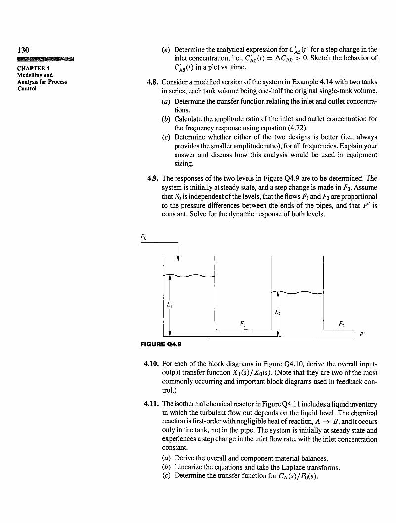
4.9. The responses of the two levels in Figure Q4.9 are to be determined. Thesystem is initially at steady state, and a step change is made in Fo. Assumethat Fo is independent of the levels, that the flows F\ and F2 are proportionalto the pressure differences between the ends of the pipes, and that P' isconstant. Solve for the dynamic response of both levels.

FIGURE Q4.9

4.10. For each of the block diagrams in Figure Q4.10, derive the overall input-output transfer function Xi (s)/Xq(s). (Note that they are two of the mostcommonly occurring and important block diagrams used in feedback control.)

4.11. The isothermal chemical reactor in Figure Q4.11 includes a liquid inventoryin which the turbulent flow out depends on the liquid level. The chemicalreaction is first-order with negligible heat of reaction, A -» B, and it occursonly in the tank, not in the pipe. The system is initially at steady state andexperiences a step change in the inlet flow rate, with the inlet concentrationconstant.id) Derive the overall and component material balances.ib) Linearize the equations and take the Laplace transforms.(c) Determine the transfer function for Ca(s)/F0(s).

ia)X0is) GAs) G2is) G3is) G4(s) Xx(s)

131

Questions

ib)X0is) ? — *■ G,(5)

+G2is) G3(s) G4is)_! i

'AO

XX(S)

FIGURE Q4.10

4.12. The frequency response of a system can be determined empirically by introducing a sine to an input variable, waiting until the initial transient isnegligible, and measuring the input and output amplitudes and the phaseangle (see Figure 4.9). If this procedure were performed for several input frequencies, how could you determine whether the real physical system were first-order or second-order? After selecting the proper transferfunction order, how could you determine the unknown parameters, gain,and time constant(s)? Also, discuss possible limitations to this empiricalmethod.

4.13. A single, isothermal, well-mixed, constant-volume CSTR is considered inthis question. The chemical reaction is

A ± > Bwhich is first-order with the forward and reverse rate constants k\ and k2,respectively. Only component A appears in the feed. The system is initiallyat steady state and experiences a step in the concentration of A in the feed.Formulate a model to describe this system, and solve for the concentrationsof A and B in the reactor.

4.14. Answer the following questions.id) The initial value of a variable can be determined in a manner similar

to the final value. Derive the general expression for the initial value.ib) The transfer function in equation (4.46) can be inverted to give

CAq(s) _ xs + 1CAis) " Kp

Discuss whether this is also a transfer function describing the process,(c) The transfer function is sometimes referred to as the impulse response

of the (linear) system. Demonstrate why this statement is true.id) If only the input-output relationship is required, why are all equations

for the system included in the model, rather than only those equationsinvolving the input and output variables?

L C *

FIGURE Q4.11

132


Th0 TCQ■1 '

n | T1 c

vh vc

FIGURE Q4.15

4.15. A heat exchanger would be difficult to model, because of the complexfluid mechanics in the shell side. To develop a simple model, consider thetwo stirred tanks in Figure Q4.15, in which heat is transferred through thecommon wall, with Q = UAiAT) and UA being constant.id) Using typical assumptions for the stirred tanks and ignoring energy

accumulation effects of the walls, derive an unsteady-state energy balance for the temperatures in both tanks.

ib) Solve for the analytical expression for both temperatures in responseto a step in 7/,o.

(c) Is it possible for this system to have periodic behavior?4.16. For the series of isothermal CSTRs in Example 3.3:

id) Derive the transfer function for CA2(s)/Fis).ib) Use this result to determine the response of Ca2 to an impulse in the

feed rate F.

4.17. The system in Figure Q4.17 has a flow of pure A to and from a drainingtank (without reaction) and a constant flow of B. Both of these flows goto an isothermal, well-mixed, constant-volume reactor with A + B ->products and rA = rB = -£CaCb. Make any additional assumptionsin determining analytical expressions for the dynamic responses from aninitial steady state.id) Determine the flow of A to the chemical reactor in response to a flow

step into the draining tank.ib) Determine the concentration of A in the chemical reactor in response

to id).

®

® ®

u

FIGURE Q4.17

4.18. The process in Figure Q4.18 involves a continuous-flow stirred tank witha mass of solid material. The assumptions for the system are:

(1) The tank is well mixed.(2) The physical properties are constant, and C„ «* Cp.(3) V = constant, F = constant [vol/time].(4) The solid material contributes a significant portion of the energy

storage, and the temperature is uniform throughout the solid.(5) The heat transfer from the liquid to the metal is UAiT — Tm).(6) Heat losses are negligible.(7) All variables are initially at steady state.

id) Determine the fundamental model equations that relate the behaviorof Tit) as 7bit) changes.

ib) Derive the Laplace transform T'is) as afunction of Tqis). This involvesthe linear(ized) deviation variables. Identify the time constants andgains,

(c) Draw a block diagram of the system of equations and derive the transferfunction Tis)/Tois).

id) State whether the system is stable or unstable and periodic or nonpe-riodic, and explain your answer.

ie) Solve the equations and sketch the dynamic response of T'it) for astep change in T it).

if) Describe briefly how the results in steps (c) through ie) would changeas UA -> oo.

133H f f l f a M M I —■

Questions

Uvcb rbT

M = massFIGURE Q4.18

modelling and analysis for process control

Documents