Modelling and Analysis of a Batch Plant Using Petri Nets

H. Yu1, T.C. Yang2, S. Cang3 and W. Chen4

1School of Informatics, Bradford University, Bradford BD7 1DP UK 2School of Engineering, University of Sussex, Falmer, Brighton, UK

3Department of Computer Science, University of Wales, Aberystwyth, SY23 3DB, UK 4Academy of Mathematics and System Sciences, Chinese Academy of Sciences, Zhongguancun Beijing 100080, P.R.China Keywords: Petri nets, Batch plant, Modelling, Performance analysis .

Abstract

Petri nets have widely been applied in different aspect of modelling, qualitative, quantitative analysis, supervisory and coordinate control, scheduling, planning, and hybrid system design of batch processes. The paper presents an example which shows how to use Petri nets to model and analysis a realistic batch plant. The modular modelling method is adopted to model a real batch processing plant with Petri nets The system properties, such as liveness, boundedness, and reversibility can be proofed by analysing each subnet. The combined Petri net model also preserves these properties. The techniques are very useful and can be also used to model the complicated batch plants.

1 Introduction

Batch processes take an important place in process industries. A batch process involves a sequence of phases that are carried out on a discrete quantity of material within a piece of operating equipment (e.g. reactors, blenders). Control of batch processes is discrete to achieve transitions between different control modes, and continuous within these modes. For example, in control of sequences and synchronisations there are two typical discrete control tasks, while the steady-state set-point control and tracking control are typical continuous control tasks. Modelling and control of dis crete event dynamics systems using Petri nets has been extensively investigated in the past three decades. Application of Petri net theory to a real life manufacturing system is a very important research area in order to develop modern manufacturing control systems. During past decade, there have been many researches conducted on Petri nets theory and applications. Petri nets have been used for modelling batch processes [1], for performing scheduling and optimisation by combining with Branch & Bound search method [5], with different types of AI based heuristics [9][10][11], with genetic algorithms [12], for panning [13]. The rule-based Petri net is developed in [6] to enhance the system decision capability. A generic Petri net is developed in [8] to enhance the Petri net modelling power. Petri nets can represent the activities, resources and constraints of such systems in a generic form. They are more

and more widely used for discrete event dynamic system modelling, scheduling and control design. There are many advantages in modelling a system using Petri nets. Examples of these advantages are: 1) They describe the mo delled system graphically and hence enable an easy visualization of complex systems [2]; 2) Petri nets can model a system hierarchically; systems can be represented in a top-down fashion at various levels of abstraction and detail [3]; 3) A systematic and qualitative analysis of the system is possible by well developed Petri net analysis techniques [2][4]; 4) Scheduling and Performance evaluation of systems is possible using timed Petri nets [4][5]. The objective of this paper is to apply Petri net techniques to a practical batch process system. This batch system is hierarchical and the control system is divided into two parts, that is, production control and process control. The former controls the plant working sequences which have a discrete-event nature and the latter controls the operation of the continuous-time plant devices. The synthesis and analysis of the first part of this batch processing system using Petri nets is presented in this paper. The Petri net concepts and modelling of the batch processing systems are briefly introduced. The batch process system running in BASF is analysed. Then the Petri net model for this system according to the above descriptions is presented. The system production rate and the utilisation of the resources in the system based on this model are investigated. The following tasks are reported in this paper:

• briefly introduce Petri net concepts and modelling, analysis and control of discrete event dynamic systems using Petri nets pertinent to the topics discussed in this paper;

• describe a batch process system running in BASF C+I Limited;

• present a Petri net model for this system according to the above descriptions;

• analyse the system production rate, investigate the utilisation of the resources in the system based on this model.

2. Petri Nets 2.1 Basic Concepts of Petri Nets In a Petri net, conditions are represented by places (circle) which are used to represent availabil i ty of resource, operations, or conditions, and events are

Control 2004, University of Bath, UK, September 2004 ID-074

represented by transitions (fil led rectangle) which are used to model the events, start , or termination of operations. Arcs indicate the relationship between places and transit ions. Tokens in places and their flow regulated by firing the enabled transit ions add the dynamics to Petri nets. Thus a marked Petri net can be used to study the dynamic behaviour of the modelled discrete event systems. A formal definit ion of a Petri net is [2][4] : [Definition 1]: A Petr i net is 5-tuple , PN=(P,T,I,O,M) where

• P={p 1 ,p 2 ,… ,p m} is a f ini te set of system states; • T={t 1 ,t 2 ,… ,t m} is a f ini te set of transit ions with

P∪T≠ 0 and P∩ T=0; • I : P× T→ N is the input (preincidence) function,

or direct arcs from P to T; • O: P× T→ N is the output (postincidence)

function or direct arcs from T to P; • M: P→N, where N={0,1,2, …}, is the M-

component marking vector whose ith component, m(p i ) is the number of tokens in the ith place. M 0 is an init ial marking.

The presence or absence of tokens indicates the status of a place, and the marking of places represents either the availabilit y of resources or the occurrence of operations. A transition t is enabled for a current marking M iff m(p i )≥I(p i , t) . An enabled transit ion may be chosen to f ire. The fir ing of the i th transit ion consists of removing I(p i , t ) tokens from each of i ts input places and adding O(p i , t) tokens to each of its output places. This yields a new marking mc(p)=m(p)-I(p,t)+O(p,t), ∀p∈ P. mc is said to be reachable from m. 2.2 Properties of Petri Nets [Definition 2:] Given a Petri net with the initial marking M 0 , t he set of all marking M’∈ PN reachable f rom M0 is called the reachabili ty set and is denoted by R(PN,M). The basic Petri net can be used to analysis the quali tative performance, such as boundedness, l iveness, and reversibil i ty of the system. Their former definit ions are: [Definition 3:] A p lace pi ∈P of a Petri net with initial marking M0 i s k-bounded if for al l M’∈PN, M’(p i )≤k . In Definit ion 2, if k=1, the PN is a safe Petri net . [Definition 4:] A Petri net with initial marking M0 is l ive if for all M’∈PN, i t is possible to ul t imately fire transit ion in the Petri net . [Definition 5:] A Petri net is reversible if for all M’∈PN then M 0 ∈R(PN,M). Based on the above definitions, there are three methods to perform the analysis using a Petri net. They are: 1) Reachability g raph method 2) Matrix equation method 3) and Reduction method

The reachabili ty graph method is fundamental to analyze the qualitative properties of the systems using a Petri net. However, it suffers from the

state explosion. The matrix equation method is ve ry useful, but i t may lose the information when the net is impure , i .e. there is a self- loop in the net . The reduction method itself is not a completed method. It translates the Petri net to a simple one and then either using the reachabil i ty method or the matrix equation method to perform the analysis . 2.3 Timed Petri Nets To perform quantitative analysis and increase the Petri net modelling power, t ime must be introduced. To add t ime to a Petri net model, the two main methods are the timed place and the t imed transition. The two methods are equivalent [2]. In this paper, the timed place model is used to preserve the convention of transit ions as instantaneous events and avoid the self loops. The formal definition is [Definition 6:] A timed Petri net, TPN=(PN,h), where • PN is a normal Petri net defined as definition 1; • h is the time delay (life -time) associated with

the relevant state. A token in a t imed place Petr i net may have two possible states: available or unavailable. In any t ime interval h, the present marking M=M a +M u , such that M a is made of available tokens and Mu is made of unavailable tokens. A transit ion is enabled if and only if M a(p i )≥I(p i ,t), where M a is the available tokens in the places. When a token arrives in a timed place, i t must remain there for a t ime interval h, to become an available token, where h is the delay time for the timed place. The t imed Petri net can be employed in a quantitative analysis, such as scheduling to either determine the minimum cycle time , or to locate bottleneck machines. 2.4 Petri Net Design Methods There are many strategies for developing Petri net models. The two main ones [3] are top-down and bot tom-up according to the differences in the p rocedures that are used to construct f inal system models. Bottom-up methods first divide the system into subsystems and specify them in detail . Then subsystems are modelled by subnets which are merged by sharing common transit ions, places, and/or paths to obtain the system model. Top-down methods, by contrast, use a macro -level model and neglect low- level detail initially. Then, the models are refined in a stepwise manner by expanding places and/or transitions to incorporate more detai ls into the models until the system is completely specified. A hybrid synthesis approach has also been formulated in which top-down refinement of operations in flexible manufacturing is fol lowed by bot tom-up modell ing of shared resources. The reali ty is often a compromise. For example, the solution could be top-down when it is obvious how to tackle the problem and bottom-up when experimentation is required to develop detailed models. A Petri net consists of places, transitions, bipartite arcs, and tokens. Places represent condit ions, which mean resource status

Control 2004, University of Bath, UK, September 2004 ID-074

(e.g. availabili ty of blenders, reactors, raw material etc.) or no resource status (e.g. operations which mean that material A and B are mixing in mixer C; intermediate storage). When they represent the former, they can be further divided into two cases. In case one, they stand for constants, e.g. , the number of blenders and reactors is f ixed; in case two, they stand for variables, e.g., the number of resource materials and products is changed depending upon the job. We call the places of case one C-places and places of case two as V-places. When they represent the later, they can also be divided into two cases, i .e. operation places where the operations are performed in the process units, and intermediate places where the in termediate material may be stored in intermediate storage (unlimited storage or f ini te storage) or process units (no-storage). The former are called O-places and the latter are called I-places. One or more tokens in a C-place or a V-place indicate that the unit (blender or reactor) or the material or the product is available and the absence of a token indicates that it is not available. A token in an O-place indicates that a job is being executed. A token in an I-place indicates that material is in intermediate storage (or wait ing in the process unit) and waits for the next process. Generally, O-places are timed places, and represent the processing time for a task. Transitions represent events which express either the start or complet ion of an operat ion and can be divided into two classes. One is a transition for the start of an operation and is called an S-transition. The rest are called E-transi t ions. Only S-transit ions can be conflict transit ions. Sometime, a n E-transit ion will also be an S-transition for the subsequent activity. Tokens reside in places and flow through transitions, which express the control logic embedded in the Petri net . 3. System Description The batch process system we studied produces two products (Terebec and Allotherm.). At the production processing, each product requires two production units (Reactor and Blender). A solvent tank farm consists of eight separate bulk storage solvent tanks. Each of them with its own header is connected (only four different solvents are used in this study for simplifying of the Petri net model) to each production unit (reactor and blender). A predetermined quantity of the required solvent is charged into a reactor or a blender via a controller / totalling control loop. The charging is controlled by a package external to distributed control system (DCS). In order to maintain the batch recipe the DCS will check if the bin identity and quantity charged complies with the recipe. The reactor required for the production is first cleaned and inserted. The suitable solvents for recipe are then charged into the reactor. If more than one solvent is needed, additions to the reactor are charged in series. Parallel charging of solvents to separate reactors is possible, but one solvent cannot be charged to several reactors simultaneously. Heating and ignition are applied to the reactor. During the heating phase, solids or more solvents

may be added. When the manufacturing steps within the reactor are finished, the product is transferred into the blender. The manufacturing steps within the blender require solids and solvent additions together with heating/cooling and agitation. At the end of blending, the product is tested, and if approved is transferred into one of the following areas.

1. Terebec can be transferred to either storage tanks, direct loading station or to the filling hall where it will be drained.

2. Allotherm can be transferred only to the filling hall for draining.

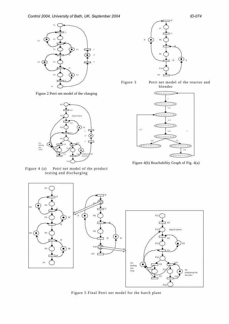
But if rejected the product would be kept in the blender to get more solvent. For the simplicity, we describe the system with one reactor and one blender. The physical model of the system is shown in Fig. 1. 4. Petri net model of the batch plant The system decomposition, refinement, and modular composition are described in terms of the synthesis process of Petri nets for the described batch plant. From Fig. 1, we can see that the batch plant consists of four parts. The first is the solvents charging, the second is the reaction part, the third is the blending, and the fourth is the product testing and discharging. We will use the modular composition methods to model the above four parts. 4.1 Modelling of Solvent Charging It is observed from Fig. 1 that there are four different kinds of solvents which are required before the reaction starts. The solvents are charged into the reactors one by one. Thus we need two places, which stand for the conditions, to model each solvent state. One place represents the solvent ready for charging and the other represents charging is in process. After charging, the solvent becomes ready again. This can be modelled using a Petri net as shown in Fig. 2. The illustration of the places and transitions of the above model is shown in Table 1.

Table 1 Illustration of places and transitions in Fig. 2. p1: Reactor available p2: Charging Solvent 1 to the reactor p3. Charging Solvent 2 to the reactor p4: Charging Solvent 3 to the reactor p5: Charging Solvent 4 to the reactor p6: Reaction in progress to the reactor S1: Solvent 1 S2: Solvent 2 S3: Solvent 3 S4: Solvent 4 t1: Start charging solvent 1 t2: Stop charging solvent 1 & start charging solvent 2 t3 : Stop charging solvent 2 & start charging solvent 3 t4: Stop charging solvent 3 & start charging solvent 4 t5: Stop charging solvent 4 & start reaction The initial marking is M0=[0 0 0 0 0 0 1 1 1 1 ]. To perform the analysis of liveness, safeness, and reversibility, an idle place p’ is initially marked with one token, and two transitions t’ and t” are associated with places p1 and p6. The resulted net is shown in Fig. 2 (see the dotted lines). It is noted that every place has exactly one input and one output transition, thus this subnet for modelling the solvent charging is a mark graph. The properties can be verified based on the facts on marked graphs [4]. Since every circuit

Control 2004, University of Bath, UK, September 2004 ID-074

in this subnet has at least one token, the net is live and reversible. Since no place have more than one token, this net is also safe. Liveness of the system means that there is no deadlock, safeness represents that there is no overflow, and reversible means that the system can go back its initial state through several actions. 4 .2 Modelling of Reactor and Blender Here, we model the reactor and blender together. The modelling sequence is that the solvents are first charged into the reactor, then the reaction takes place, after the reaction, it is discharged from the reactor and is charged into the blender, Finally, it is tested and is discharged to the filling tank. This is modelled in Fig. 3. The meaning of the places and transitions of the above model is shown in Table 2. The initial marking of this Petri net is [0 0 0 0 1 1 ]. It is noted that places p7 and p10 are macro-places which represent charging, testing and discharging. This Petri net is also a marked graph. there is a token and only a token in every circuit. Thus the Petri net is live, safe, and reversible.

Table 2 Illustration of places and transitions in Fig. 3. p7: Charging solvents p8: Reaction in progress to the reactor p9: Discharging reactor & charging blender p10: Blending&testing&discharging R: Reactor available B: Blender available t6: Start charging solvents t7: Stop charging solvents & start reaction t8 : Stop reaction&start charging blender t9: Stop charging&discharging & start blending t10: Stop discharging blender 4.3 Modelling of Quality Test The Petri net model of this part is shown in Fig. 4(a). The product is tested by an operator, O1 . The result is either accepted (i t can be discharged), p17 or rejected (it must charge more solvent and blending again) , p1 6 . This means that there is a choice in this net structure. In order to model the rework of the rejected product, a logic place, p1 3 , is introduced. The meaning of the places and transitions of the above model is shown in Table 3.

Table 3 Illustration of places and transitions in Fig. 4(a). p12: Ready for blending p13: Logical place for rejected material p14: Blending p15: Testing p16: Testing fail & require reblending p17: Testing success & discharging blender S5: Blending resource available O1: Operator available for testing O2: Operator available for discharging t12: Pumping to blender finish t13: Start blending t14 : Stop blending & start testing t15: testing finish (fail) t16: testing finish (success) & start discharging blender t17: Start reblending t16: Discharging finish The initial marking is [0 0 0 0 0 0 1 1 1]T. We can first introduce a dump place with two transitions as in Section 4.1 and construct a reachability graph of this Petri net shown

in Fig. 4(b). We can prove that this net is live, reversible and safe using the reachability graph shown in Fig. 4(b). 4.4 Combined Petri Nets The final Petri net is obtained by refining the p l aces p7 a n d p10 in Fig. 3 by the nets shown in Figs 2 and 4(a), respectively. Since both detailed nets in Figs 2 and 4(a) are live, reversible, and safe, these two refinements guarantee the resulting the final net to be l ive, reversible, and safe [2][4] . The combined Petri net is shown in Fig. 5. 5. Analysis of Timed Petri Nets

Performance evaluation of a batch production system provides the ability to perceive clearly the production plan of the system. It is used to identify the bottleneck in the production unit, estimate the raw material required for production and decide operating policies. Evaluation of the performance of a batch production system is not easy, because of the concurrent nature of the activities. A Petri Net model is convenient for evaluating the performance of a batch production process for one product flowing sequentially through a production line. As Petri Net model of the logical and casual dependencies in manufacturing system is not a sufficient tool to analyse the characteristics of the system such as time, resource availability, capacity and demand, we have introduced the concept of timed Petri net. Time to charge each solvent in Fig 2 is about 30 min. The total time for charging four solvents into the reactor is about 120 min and this can be reflected as a delay time in place p7. The time for reaction is 1080 min which represents the delay time in p8. The time for discharging the reactor/charging the blender is 60 min which represents the delay time in p9. The time for blending is 360 min. The time for testing and discharging is about 180 min. The delay time in p10 represents the sum of the blending time and the time for testing and discharging. It is noted that it is difficult to compute the accurate time for testing and reworking since the random nature exists in this task. To deal with this properly, the stochastic Petri net is required. This is beyond of the work reported here. We define an elementary circuit in a strongly connected graph as a directed path that goes back to the same node, while any other node is not repeated. Every place in a marked graph is restricted to being an input/output of exactly one transition. When the times are deterministic as in our example, we can compute, for any elementary circuit g, the following ratio called the cycle time of the circuit [2][4]: Cg = m(g)/M(g) For the marked graph, the minimum cycle time, Cm is Cm = Max { m(g)/M(g) } for g = { 1....q }

where q is the number of circuits in the model, m(g) is the sum of place delays in the circuit g, M(g) is the sum of tokens in the circuit g. Let us now calculate the cycle time of our model in order to find out the minimum cycle time or maximum performance of the production units in this system. To compute the result, it is important to list all the circuits produced by this model and show the minimum cycle time

Control 2004, University of Bath, UK, September 2004 ID-074

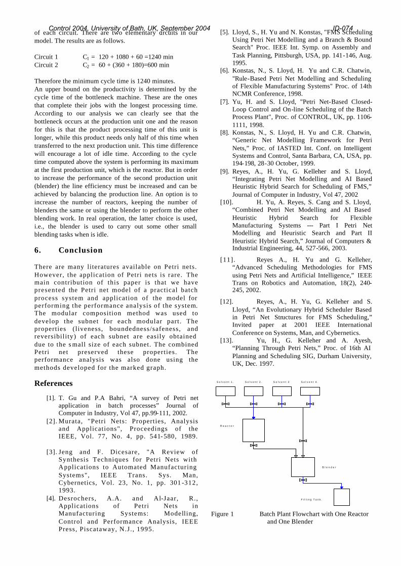
of each circuit. There are two elementary circuits in our model. The results are as follows. Circuit 1 C1 = 120 + 1080 + 60 =1240 min Circuit 2 C2 = 60 + (360 + 180)=600 min Therefore the minimum cycle time is 1240 minutes. An upper bound on the productivity is determined by the cycle time of the bottleneck machine. These are the ones that complete their jobs with the longest processing time. According to our analysis we can clearly see that the bottleneck occurs at the production unit one and the reason for this is that the product processing time of this unit is longer, while this product needs only half of this time when transferred to the next production unit. This time difference will encourage a lot of idle time. According to the cycle time computed above the system is performing its maximum at the first production unit, which is the reactor. But in order to increase the performance of the second production unit (blender) the line efficiency must be increased and can be achieved by balancing the production line. An option is to increase the number of reactors, keeping the number of blenders the same or using the blender to perform the other blending work. In real operation, the latter choice is used, i.e., the blender is used to carry out some other small blending tasks when is idle. 6. Conclusion There are many literatures available on Petri nets. However, the application of Petri nets is rare. The main contribution of this paper is that we have presented the Petri net model of a practical batch process system and application of the model for performing the performance analysis of the system. The modular composition method was used to develop the subnet for each modular part . The properties (l iveness, boundedness/safeness, and reversibil i ty) of each subnet are easily obtained due to the s mall size of each subnet. The combined Petri net preserved these properties. The performance analysis was also done using the methods developed for the marked graph. References

[1]. T. Gu and P.A Bahri, “A survey of Petri net application in batch processes” Journal of Computer in Industry, Vol 47, pp.99-111, 2002.

[2]. Murata, "Petri Nets: Properties, Analysis and Applications", Proceedings of the IEEE, Vol. 77, No. 4, pp. 541- 580, 1989.

[3]. Jeng and F. Dicesare, "A Review of Synthesis Techniques for Petri Nets with Applications to Automated Manufacturing Systems", IEEE Trans. Sys. Man, Cybernetics, Vol. 23, No. 1, pp. 301 -312, 1993.

[4]. Desrochers , A.A. and Al-Jaar, R. , Applications of Petri Nets in Manufacturing Systems: Modelling, Control and Performance Analysis, IEEE Press, Piscataway, N.J. , 1995.

[5]. Lloyd, S., H. Yu and N. Konstas, "FMS Scheduling Using Petri Net Modelling and a Branch & Bound Search" Proc. IEEE Int. Symp. on Assembly and Task Planning, Pittsburgh, USA, pp. 141-146, Aug. 1995.

[6]. Konstas, N., S. Lloyd, H. Yu and C.R. Chatwin, "Rule-Based Petri Net Modelling and Scheduling of Flexible Manufacturing Systems" Proc. of 14th NCMR Conference, 1998.

[7]. Yu, H. and S. Lloyd, "Petri Net-Based Closed-Loop Control and On-line Scheduling of the Batch Process Plant", Proc. of CONTROL, UK, pp. 1106-1111, 1998.

[8]. Konstas, N., S. Lloyd, H. Yu and C.R. Chatwin, “Generic Net Modelling Framework for Petri Nets,” Proc. of IASTED Int. Conf. on Intelligent Systems and Control, Santa Barbara, CA, USA, pp. 194-198, 28-30 October, 1999.

[9]. Reyes, A., H. Yu, G. Kelleher and S. Lloyd, “Integrating Petri Net Modelling and AI Based Heuristic Hybrid Search for Scheduling of FMS,” Journal of Computer in Industry, Vol 47, 2002

[10]. H. Yu, A. Reyes, S. Cang and S. Lloyd, “Combined Petri Net Modelling and AI Based Heuristic Hybrid Search for Flexible Manufacturing Systems --- Part I Petri Net Modelling and Heuristic Search and Part II Heuristic Hybrid Search,” Journal of Computers & Industrial Engineering, 44, 527-566, 2003.

[11]. Reyes A., H. Yu and G. Kelleher, “Advanced Scheduling Methodologies for FMS using Petri Nets and Artificial Intelligence,” IEEE Trans on Robotics and Automation, 18(2), 240-245, 2002.

[12]. Reyes, A., H. Yu, G. Kelleher and S. Lloyd, “An Evolutionary Hybrid Scheduler Based in Petri Net Structures for FMS Scheduling,” Invited paper at 2001 IEEE International Conference on Systems, Man, and Cybernetics.

[13]. Yu, H., G. Kelleher and A. Ayesh, “Planning Through Petri Nets,” Proc. of 16th AI Planning and Scheduling SIG, Durham University, UK, Dec. 1997.

S o l v e n t 1 . S o l v e n t 2 . S o l v e n t 3 . S o l v e n t 4 .

R e a c t o r

B l e n d e r

F i l l i n g T a n k .

Figure 1 Batch Plant Flowchart with One Reactor

and One Blender

Control 2004, University of Bath, UK, September 2004 ID-074

S 1

S 2

S 3

S 4

P 1

P 2

P 3

P 4

P 5

t1

t2

t3

t4

t5

P 6

p '

t '

t"

Figure 2 Petri net model of the charging

logical place

S5

P12

P13

P14

P15

P16 P 1 7

t 1 2

t 1 3

t 1 4

t 1 5t 1 6

t 1 7 t 1 8

O 1testingthe f ina lproduct O 2

emptiying the b lender

P 1 9

t '

t"

p "

Figure 4 (a) Petri net model of the product

test ing and discharging

R

B

P7

P8

P9

P 1 0

t6

t7

t8

t9

t10

Figure 3 Petri net model of the reactor and

blender

0 0 0 0 0 0 0 1 1 1 1

1 0 0 0 0 0 0 1 1 1 0

0 1 0 0 0 0 0 1 1 1 0

0 0 1 0 0 0 0 0 1 1 0

0 0 0 1 0 0 0 1 0 1 0

0 0 0 0 1 0 0 1 1 1 0 0 0 0 0 0 1 0 1 1 0 0

0 0 0 0 0 0 1 1 1 1 0

t '

t 1 2

t 1 3

t 1 4

t 1 5 t 1 6

t 1 7 t"

t 1 8

Figure 4(b) Reachability Graph of Fig. 4(a)

R

B

P7

P8

P9

P10

t6

t7

t8

t9

t 1 0

S1

S2

S3

S4

P1

P2

P3

P4

P5

t1

t2

t3

t4

t5

P6

logical place

S5

P12

P13

P14

P15

P16 P17

t12

t13

t14

t15t 1 6

t17 t 1 8

O 1testingthe finalproduct

O2emptiying the b lender

P19

Figure 5 Final Petri net model for the batch plant

Control 2004, University of Bath, UK, September 2004 ID-074