modelling and cfd simulation of hydrodynamics and … · computational fluid dynamics (cfd) was...
TRANSCRIPT
International Journal of Engineering and Technology sciences (IJETS) 2 (3): 223-242, 2014 ISSN 2289-4152 © Academic Research Online Publisher
Research Article
Modelling and CFD Simulation of Hydrodynamics and Mass Transfer in a
Miniature Bubble Column Bioreactor
Soheila Kheradmandnia, Seyyed Mohammad Mousavi *, Sameereh Hashemi-Najafabadi **,
Seyed Abbas Shojaosadati
Biotechnology Group, Chemical Engineering Faculty, Tarbiat Modares University, P.O.Box: 14115-114,
Tehran, Iran
* Corresponding author: Biotechnology Group, Chemical Engineering Faculty, Tarbiat Modares University,
P.O.Box: 14115-114, Tehran, Iran, Tel.: +98-21-82884917; Fax: +98-21-82884931
E-mail address: [email protected]
** Corresponding author: Biotechnology Group, Chemical Engineering Faculty, Tarbiat Modares University,
P.O.Box: 14115-114, Tehran, Iran, Tel.: +98-21-82884384; Fax: +98-21-82884931
E-mail address: [email protected]
A b s t r a c t
Keywords:
Computational fluid
dynamics (CFD),
Flow pattern,
Miniature bubble column
bioreactor(MBCR),
Volumetric mass transfer
coefficient (LK a ).
Computational fluid dynamics (CFD) was used to study a 3D simulation of
hydrodynamics and mass transfer in a miniature bubble column bioreactor
(MBCR). The ability of a two-fluid phase model to predict flow behaviour was
studied by applying the laminar and turbulence models. The volumetric mass
transfer coefficient (KLa) was predicted at different superficial gas velocities and
sparger pore sizes. The simulation results of KLa showed a good agreement with
the experimental data in a 30 μm sparger pore size. A similar behaviour was
observed in the liquid circulation, gas distribution and their relation in the MBCR
like as large scale bubble columns. Increasing the superficial gas velocity led to an
increase in the liquid circulation near the walls, followed by an increase of the gas
holdup and KLa. Decreasing the pore size of sparger produced smaller bubbles
which resulted in increased gas holdup and KLa. Linear relation between the
superficial gas velocity and interfacial area was investigated as the same as a short
bubble columns. Observation of the similar behaviour in the hydrodynamic
characteristics of traditional and miniature scales of the bubble columns may
encourage the researchers to develop the MBCRs in the high throughput
processes.
Accepted:26 April2014 © Academic Research Online Publisher. All rights reserved.
Kheradmandnia, S. et al. / International Journal of Engineering and Technology sciences (IJETS) 2 (3): 223-242, 2014
224 | P a g e
Nomenclature
General Symbols a Interfacial area (m
-1) Reb
Bubble Reynolds number
DC Drag force coefficient 0
0
4Re L
L
L
Q
d
Modified sparger Reynolds number
LC Concentration of dissolved oxygen (Kg.m-3
) S Interphase mass transfer (Kg.m-3
s-1
)
LC Saturation concentration of dissolved
oxygen (Kg.m-3
) L
L
ScD
Schmitt number
LC
Steady state concentration of dissolved
oxygen (Kg.m-3
) Sh Sherwood number
liftC Lift force coefficient t Time (s)
C Coefficient for turbulence viscosity u Velocity (m.s
-1)
1 2,C C Constants in k–ε model
D
Diffusion coefficient (m2.s
-1)
0d
Sparger pore size (m, μm) Greek Symbols
bd
Average bubble diameter (m) Phase volume fraction
Eo
Eötvös number eff Effective viscosity (pa.s
-1)
F
Interfacial force between liquid and gas
phase (N.m-3
)
Density (kg.m-3
)
DF
Drag force (N.m-3
) Turbulence dissipation rate of specific
phase (m2.s
-3)
LiftF
Lift force (N.m-3
) Surface tension (N.m-1
)
2
0
0
QFr
g d
Sparger Froude number
g Gravitational acceleration (ms-2
) Subscripts
k Turbulence kinetic energy of specific phase
(m2.s
-2)
b Bubble
LK Liquid mass transfer coefficient (ms-1
) D Drag
OUR Oxygen Uptake Rate (Kg.m-3
s-1
) G Gas
P Pressure (pa) k Phase
L Liquid
1. Introduction
In recent years, bioprocess development such as screening and optimization has been performed at
small scale systems [1]. Scaling down the volume of the bioreactors, performing parallel bioprocesses
and on-line monitoring the experiments create a good opportunity for saving in time, materials and
labor intensity [2]. Ability of the miniature bioreactors to examine a wide range of experimental
conditions and select the optimized conditions, makes them as high-throughput systems for bioprocess
development [3]. Parallel MBCRs are one of the suitable candidates for medium or strain
improvement and early-stage process development beside the other small scale systems [4]. Similar to
laboratory and large scale bubble columns, miniature columns are mechanically simple and their final
Kheradmandnia, S. et al. / International Journal of Engineering and Technology sciences (IJETS) 2 (3): 223-242, 2014
225 | P a g e
design cost is less than stirred tanks. They can be easily instrumented, automated and characterized [5,
6].
In the bubble column bioreactors, operation is performed via contact between gas and liquid phase.
Aeration and mixing are achieved by gas sparging from the bottom of the column. Sparger type,
superficial gas velocity and bubble size distribution as the main factors affect the transport
phenomena in these devices [7]. Sparger type and gas flow rate affect the size and behavior of the
released bubbles from the sparger, gas hold up, fluid mixing and oxygen transfer rate [8]. Despite the
simple design, the flow behaviour is complicated in the bubble columns. Three flow regimes occur in
these columns depending on the inlet gas flow rate and column diameter [9]. At low superficial gas
velocities (< 0.05 m.s-1
), homogeneous or bubbly flow is dominant in the column. In the
homogeneous regime, bubbles are small with a uniform distribution. Turbulence and bubble
coalescing or breaking can be neglected. Liquid circulation is small and finally the radial profiles of
gas hold up and liquid velocity is obtained. By increasing the superficial gas velocity, heterogeneous
condition is dominant in the system. In a heterogeneous regime, the bubble swarming occurs which is
directed towards the wall of the bioreactor. Large bubbles are formed by coalescence depending on
the column diameter. The recirculation rate in the vessel is increased, extensively. Hold up and liquid
velocity magnitude are at the maximum values at the center of the column and their profiles are
parabolic with the sharp peak. The third regime is the intermediate regime that is called transition
flow regime. This regime exists between the homogeneous and heterogeneous flows. The major
phenomenon in the transition flow is the coalescence and formation of larger bubbles rather than
homogeneous flow [6].
Performance of the bubble column reactors is determined by the flow regime and mass and
momentum transfer in the column [10]. Over the last few years, computational fluid dynamics (CFD)
have found a widespread application to describe the flow hydrodynamics and mass transfer in many
bioreactors, especially bubble columns [11, 12]. However, modelling of transport phenomena in the
miniature bioreactors is still rare. Lamping et al., successfully modelled liquid and gas speed, energy
dissipation rate, gas hold up and LK a in a miniature stirred tank bioreactor by CFD simulations [13].
Zhang et al., applied CFD to a single well of both 24-well and 96-well microtiter plates [14]. The
liquid velocity, gas liquid interface, power consumption and energy dissipation rate were predicted in
a well of microtiter plate during orbital shaking. Rihani et al., used CFD in a milli torus reactor with
k turbulent model to simulate flow pattern, turbulence and gas hold up profiles [15]. There is no
report on the CFD simulation of miniature bubble column bioreactors in literatures. Therefore, to
observe the potential of computational techniques in prediction of flow and mass transfer in the small
scale bioreactors, hydrodynamics and LK a have been simulated in the MBCR with 2 mL working
Kheradmandnia, S. et al. / International Journal of Engineering and Technology sciences (IJETS) 2 (3): 223-242, 2014
226 | P a g e
volume. Possible similarities and differences between the large and small scales of the bubble
columns are also investigated. To validate the model, results have been compared against the
experimental data presented by Doig et al., [16].
2. Experimental procedures
2.1. Geometry and grid of the miniature column
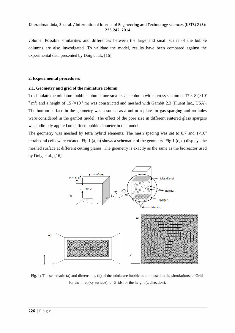
To simulate the miniature bubble column, one small scale column with a cross section of 17 × 8 (×10-
6 m
2) and a height of 15 (×10
-3 m) was constructed and meshed with Gambit 2.3 (Fluent Inc., USA).
The bottom surface in the geometry was assumed as a uniform plate for gas sparging and no holes
were considered in the gambit model. The effect of the pore size in different sintered glass spargers
was indirectly applied on defined bubble diameter in the model.
The geometry was meshed by tetra hybrid elements. The mesh spacing was set to 0.7 and 1×10⁵
tetrahedral cells were created. Fig.1 (a, b) shows a schematic of the geometry. Fig.1 (c, d) displays the
meshed surface at different cutting planes. The geometry is exactly as the same as the bioreactor used
by Doig et al., [16].
Fig. 1: The schematic (a) and dimensions (b) of the miniature bubble column used in the simulations. c: Grids
for the inlet (xy surface); d: Grids for the height (z direction).
Kheradmandnia, S. et al. / International Journal of Engineering and Technology sciences (IJETS) 2 (3): 223-242, 2014
227 | P a g e
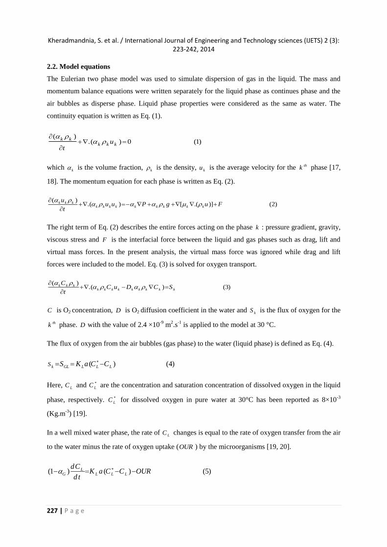
2.2. Model equations
The Eulerian two phase model was used to simulate dispersion of gas in the liquid. The mass and
momentum balance equations were written separately for the liquid phase as continues phase and the
air bubbles as disperse phase. Liquid phase properties were considered as the same as water. The
continuity equation is written as Eq. (1).
( ).( ) 0 (1)
k kk k ku
t
which k is the volume fraction,
k is the density, ku is the average velocity for the thk phase [17,
18]. The momentum equation for each phase is written as Eq. (2).
( ).( ) [ .( )] (2)k k k
k k k k k k k k k
uu u P g u F
t
The right term of Eq. (2) describes the entire forces acting on the phase k : pressure gradient, gravity,
viscous stress and F is the interfacial force between the liquid and gas phases such as drag, lift and
virtual mass forces. In the present analysis, the virtual mass force was ignored while drag and lift
forces were included to the model. Eq. (3) is solved for oxygen transport.
( ).( ) (3)k k k
k k k k k k k k k
CC u D C S
t
C is O2 concentration, D is O2 diffusion coefficient in the water and kS is the flux of oxygen for the
thk phase. D with the value of 2.4 ×10⁻⁹
m2.s
-1 is applied to the model at 30 °C.
The flux of oxygen from the air bubbles (gas phase) to the water (liquid phase) is defined as Eq. (4).
( ) (4)k GL L L LS S K a C C
Here, LC and *
LC are the concentration and saturation concentration of dissolved oxygen in the liquid
phase, respectively. *
LC for dissolved oxygen in pure water at 30°C has been reported as 8×10⁻³
(Kg.m-3
) [19].
In a well mixed water phase, the rate of LC changes is equal to the rate of oxygen transfer from the air
to the water minus the rate of oxygen uptake (OUR ) by the microorganisms [19, 20].
(1 ) ( ) (5)LG L L L
dCK a C C OUR
d t
Kheradmandnia, S. et al. / International Journal of Engineering and Technology sciences (IJETS) 2 (3): 223-242, 2014
228 | P a g e
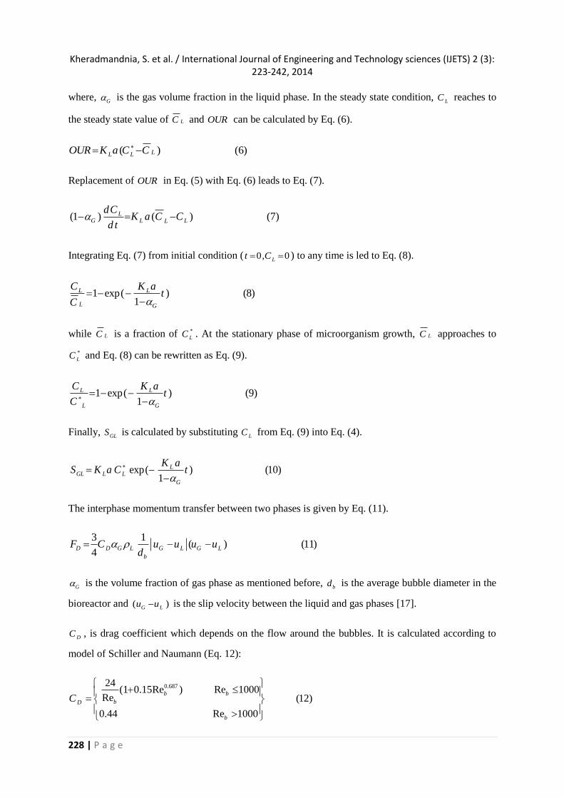
where, G is the gas volume fraction in the liquid phase. In the steady state condition,
LC reaches to
the steady state value of LC and OUR can be calculated by Eq. (6).
( ) (6)LL LOUR K a C C
Replacement of OUR in Eq. (5) with Eq. (6) leads to Eq. (7).
(1 ) ( ) (7)LG L LL
dCK a C C
d t
Integrating Eq. (7) from initial condition ( 0, 0Lt C ) to any time is led to Eq. (8).
1 exp( ) (8)1
L L
L G
C K at
C
while LC is a fraction of *
LC . At the stationary phase of microorganism growth, LC approaches to
*
LC and Eq. (8) can be rewritten as Eq. (9).
1 exp( ) (9)1
L L
L G
C K at
C
Finally, GLS is calculated by substituting LC from Eq. (9) into Eq. (4).
exp( ) (10)1
LGL L L
G
K aS K a C t
The interphase momentum transfer between two phases is given by Eq. (11).
3 1( ) (11)
4D D G L G L G L
b
F C u u u ud
G is the volume fraction of gas phase as mentioned before, bd is the average bubble diameter in the
bioreactor and ( )G Lu u is the slip velocity between the liquid and gas phases [17].
DC , is drag coefficient which depends on the flow around the bubbles. It is calculated according to
model of Schiller and Naumann (Eq. 12):
0.68724
(1 0.15Re ) Re 1000Re (12)
0.44 Re 1000
b b
bD
b
C
Kheradmandnia, S. et al. / International Journal of Engineering and Technology sciences (IJETS) 2 (3): 223-242, 2014
229 | P a g e
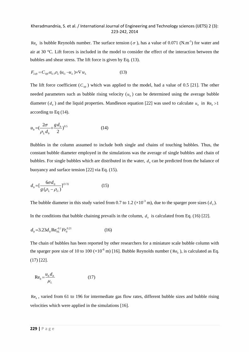
Reb is bubble Reynolds number. The surface tension ( ), has a value of 0.071 (N.m
-1) for water and
air at 30 °C. Lift forces is included in the model to consider the effect of the interaction between the
bubbles and shear stress. The lift force is given by Eq. (13).
( ) (13)Lift lift G L G L LF C u u u
The lift force coefficient (liftC ) which was applied to the model, had a value of 0.5 [21]. The other
needed parameters such as bubble rising velocity (bu ) can be determined using the average bubble
diameter (bd ) and the liquid properties. Mandleson equation [22] was used to calculate
bu in Re 1b
according to Eq (14).
0.52( ) (14)
2
bb
L b
gdu
d
Bubbles in the column assumed to include both single and chains of touching bubbles. Thus, the
constant bubble diameter employed in the simulations was the average of single bubbles and chain of
bubbles. For single bubbles which are distributed in the water, bd can be predicted from the balance of
buoyancy and surface tension [22] via Eq. (15).
(1/3)06[ ] (15)
( )b
L G
dd
g
The bubble diameter in this study varied from 0.7 to 1.2 (×10-3
m), due to the sparger pore sizes (0d ).
In the conditions that bubble chaining prevails in the column, bd is calculated from Eq. (16) [22].
0.1 0.21
0 0 03.23 Re (16)b Ld d Fr
The chain of bubbles has been reported by other researchers for a miniature scale bubble column with
the sparger pore size of 10 to 100 (×10-6
m) [16]. Bubble Reynolds number ( Reb ), is calculated as Eq.
(17) [22].
Reb , varied from 61 to 196 for intermediate gas flow rates, different bubble sizes and bubble rising
velocities which were applied in the simulations [16].
Re (17)b bb
L
u d
Kheradmandnia, S. et al. / International Journal of Engineering and Technology sciences (IJETS) 2 (3): 223-242, 2014
230 | P a g e
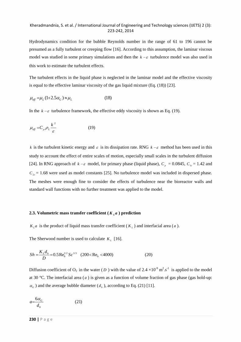
Hydrodynamics condition for the bubble Reynolds number in the range of 61 to 196 cannot be
presumed as a fully turbulent or creeping flow [16]. According to this assumption, the laminar viscous
model was studied in some primary simulations and then the k turbulence model was also used in
this work to estimate the turbulent effects.
The turbulent effects in the liquid phase is neglected in the laminar model and the effective viscosity
is equal to the effective laminar viscosity of the gas liquid mixture (Eq. (18)) [23].
(1 2.5 ) (18)eff L G L
In the k turbulence framework, the effective eddy viscosity is shown as Eq. (19).
k is the turbulent kinetic energy and is its dissipation rate. RNG k method has been used in this
study to account the effect of entire scales of motion, especially small scales in the turbulent diffusion
[24]. In RNG approach of k model, for primary phase (liquid phase), C = 0.0845, 1C = 1.42 and
2C = 1.68 were used as model constants [25]. No turbulence model was included in dispersed phase.
The meshes were enough fine to consider the effects of turbulence near the bioreactor walls and
standard wall functions with no further treatment was applied to the model.
2.3. Volumetric mass transfer coefficient (L
K a ) prediction
LK a is the product of liquid mass transfer coefficient (LK ) and interfacial area ( a ).
The Sherwood number is used to calculate LK [16].
1/2 1/30.5Re (200 Re 4000) (20)L bb b
K dSh Sc
D
Diffusion coefficient of O2 in the water ( D ) with the value of 2.4 ×10⁻⁹
m2.s
-1 is applied to the model
at 30 °C. The interfacial area ( a ) is given as a function of volume fraction of gas phase (gas hold-up:
G ) and the average bubble diameter (bd ), according to Eq. (21) [11].
6(21)G
b
ad
2
(19)eff L
kC
Kheradmandnia, S. et al. / International Journal of Engineering and Technology sciences (IJETS) 2 (3): 223-242, 2014
231 | P a g e
2.4. Numerical implementation
2.4.1. CFD model set up
Fluent as a commercial code was used to solve three dimensional governing equations. FLUENT 6.3
installed in a supercomputer system with two processors (each processor contained 12 cores) and 32
GB available RAM. The CFD model was solved with parallelization technique that has been
described in detail in the Fluent user guide [25]. The Eulerian two phase method, both of laminar and
turbulent flow regimes and unsteady state condition were also included in the model. The air was
selected as a unit component in the model. Thus, to consider the oxygen transfer from the air to the
water, oxygen concentration was expressed according to the LK a parameter. A user define function
(UDF) was implemented to the software to calculate oxygen concentration, LK a and GLS using the
equations discussed in sections 2.2 and 2.3. Unsteady state formulation and pressure-velocity coupling
were set to the first-order implicit and phase-coupled SIMPLE respectively. First-order upwind was
chosen for momentum, volume fraction and turbulent parameters. Under-relaxation factors for
pressure, momentum, volume fraction, turbulent kinetic energy, turbulent dissipation rate and
turbulent viscosity were set to 0.5, 0.7, 0.5, 0.7, 0.7 and 0.7, respectively. Time step and convergence
criterion for each scale residual component were specified as 1× 10⁻⁴
through the simulation. LK a was
obtained when the simulations reached to steady state and total gas hold up in the column remained at
a constant level.
2.4.2. Boundary conditions
The bottom plate of the column was modelled as a uniform gas inlet. The inlet gas velocity was equal
to the superficial gas velocity to consider the existence of many supposed pores on the plate.
The pressure outlet was chosen for outlet and no-slip boundary condition was applied to the walls.
The turbulence intensity for the boundary conditions was set at 0.05% to achieve low turbulence
system [25] which was near the laminar conditions.
3. Results and Discussion
3.1. Choosing the suitable viscous model
Homogeneous flow behavior is dominant in the columns with the small diameter and low superficial
gas velocity [5, 26]. Therefore, at the first step, the laminar (homogeneous) flow regime was
considered in the model. By applying the laminar model the characteristics of a turbulent regime such
Kheradmandnia, S. et al. / International Journal of Engineering and Technology sciences (IJETS) 2 (3): 223-242, 2014
232 | P a g e
as sharp peak of gas hold up in the center line was observed unexpectedly (results have not been
shown). It showed that this model had low ability to predict reasonable results for the simulations.
Other researchers have also reported the same heterogeneous behaviour when they used the laminar
model in simulation of laboratory scale bubble columns [27, 28]. Sokolichin et al., showed that by
increasing the grid refinement in their reactor with laminar model, convergence in the solution was
not gained and the number of circulation cells grows continuously. Grid dependency of the results is
not reliable. Therefore, they studied k model to apply the effect of small eddies and found that in
2D version of k model, the grid independent solution was achieved but the dynamic nature of
flow was not reproduced. According to their investigations, the experimental data were in the
agreement with the results of 3D turbulent model [23]. 2D and 3D versions of k model for
simulating the systems with low Reynolds number were used also by other researchers. For example
Mudde et al., observed the steady state solution in a 2D simulation of their bubble column, but
turbulent viscosity was high and the bubble plume was attached to the wall. It was caused by
overestimation of the turbulent viscosity. At the next step, using a 3D simulation, the small liquid
circulation was observed and the flow approached to the transient regime [29].
However some studies neglected the effect of virtual mass or lift forces in the simulation of the bubble
columns [29-31], but others studied the effect of these interfacial forces on the stability and reliability
of the hydrodynamic simulations in the bubble columns. Delnoij et al., applied drag, lift and virtual
mass forces to simulate the hydrodynamics behaviour of a laminar flow in a bubble column [32]. In
the simulated flow profiles of a bubble coumn studied by Monahan et al., all the interfacial forces had
significant role [21]. Silva et al., studied the effect of interfacial forces and turbulence models in a
bubble column to evaluate the flow pattern in the heterogeneous and homogeneous regimes [33].
The present work was followed by a 3D version of "RNG" k turbulence model to consider the
effect of turbulence formed and spread by small eddies in low Reynolds number. Drag and lift forces
were added to the model and the virtual mass force was neglected to avoid the instability of the
solution.
3.2. The effect of grid size on the simulation results
For checking the grid independency, three different grids were used. The mesh spacing was set to 1.0
for the first grid as a coarse grid and 6×10⁴ tetrahedral elements were created. The second grid was
finer and contained 1×10⁵ tetrahedral elements with 0.7 mesh spacing. The third grid was the finest
one with 0.5 mesh spacing and 2×10⁵ tetrahedral elements. The grid independency checking was done
Kheradmandnia, S. et al. / International Journal of Engineering and Technology sciences (IJETS) 2 (3): 223-242, 2014
233 | P a g e
at a constant sparger pore size of 30 μm and superficial gas velocity of 0.004 m.s-1
. The results of gas
volume fraction as well as the liquid and gas velocities were recorded for all 3 cases in 5 seconds
simulating. In this point the system reached to the stabilization. Total gas hold up and velocity profiles
reached to a constant level and no significant changing was observed during the further iterations. The
comparison of the calculated data with different grid sizes has been depicted in Table 1.
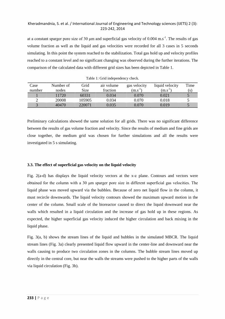
Table 1: Grid independency check.
Case
number
Number of
nodes
Grid
Size
air volume
fraction
gas velocity
(m.s-1
)
liquid velocity
(m.s-1
)
Time
(s)
1 11720 60331 0.034 0.070 0.021 5
2 20008 105905 0.034 0.070 0.018 5
3 40470 220071 0.035 0.070 0.019 5
Preliminary calculations showed the same solution for all grids. There was no significant difference
between the results of gas volume fraction and velocity. Since the results of medium and fine grids are
close together, the medium grid was chosen for further simulations and all the results were
investigated in 5 s simulating.
3.3. The effect of superficial gas velocity on the liquid velocity
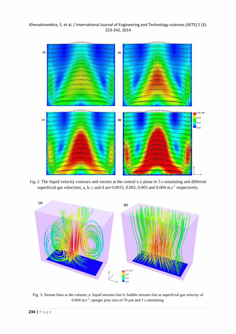
Fig. 2(a-d) has displays the liquid velocity vectors at the x-z plane. Contours and vectors were
obtained for the column with a 30 μm sparger pore size in different superficial gas velocities. The
liquid phase was moved upward via the bubbles. Because of zero net liquid flow in the column, it
must recircle downwards. The liquid velocity contours showed the maximum upward motion in the
center of the column. Small scale of the bioreactor caused to direct the liquid downward near the
walls which resulted in a liquid circulation and the increase of gas hold up in these regions. As
expected, the higher superficial gas velocity induced the higher circulation and back mixing in the
liquid phase.
Fig. 3(a, b) shows the stream lines of the liquid and bubbles in the simulated MBCR. The liquid
stream lines (Fig. 3a) clearly presented liquid flow upward in the center-line and downward near the
walls causing to produce two circulation zones in the columns. The bubble stream lines moved up
directly in the central core, but near the walls the streams were pushed to the higher parts of the walls
via liquid circulation (Fig. 3b).
Kheradmandnia, S. et al. / International Journal of Engineering and Technology sciences (IJETS) 2 (3): 223-242, 2014
234 | P a g e
Fig. 2: The liquid velocity contours and vectors at the central x-z plane in 5 s simulating and different
superficial gas velocities; a, b, c and d are 0.0015, 0.002, 0.003 and 0.004 m.s-1
respectively.
Fig. 3: Stream lines at the column; a: liquid streams line b: bubble streams line at superficial gas velocity of
0.004 m.s-1
, sparger pore size of 30 μm and 5 s simulating.
Kheradmandnia, S. et al. / International Journal of Engineering and Technology sciences (IJETS) 2 (3): 223-242, 2014
235 | P a g e
This flow behaviour was also investigated by Delnoij et al., for simulating a short bubble column with
cross section of 0.175×0.175 m2 and the ratio of height to diameter (aspect ratio) smaller than 1.0
[34]. For larger bubble columns with aspect ratio more than 1.0, the flow field changed to a more
complex with s-shaped path through the column or shifted from left to right and vise versa at fully
turbulent regime [35, 36].
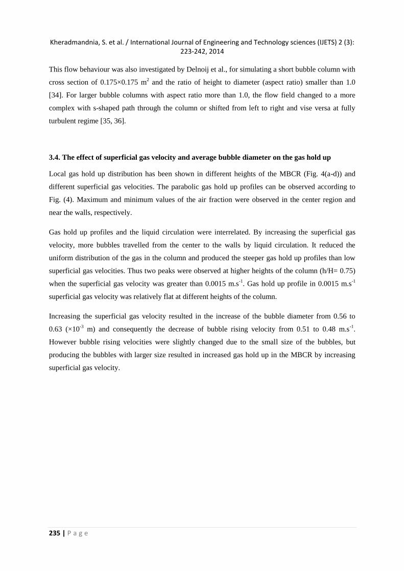
3.4. The effect of superficial gas velocity and average bubble diameter on the gas hold up
Local gas hold up distribution has been shown in different heights of the MBCR (Fig. 4(a-d)) and
different superficial gas velocities. The parabolic gas hold up profiles can be observed according to
Fig. (4). Maximum and minimum values of the air fraction were observed in the center region and
near the walls, respectively.
Gas hold up profiles and the liquid circulation were interrelated. By increasing the superficial gas
velocity, more bubbles travelled from the center to the walls by liquid circulation. It reduced the
uniform distribution of the gas in the column and produced the steeper gas hold up profiles than low
superficial gas velocities. Thus two peaks were observed at higher heights of the column (h/H= 0.75)
when the superficial gas velocity was greater than 0.0015 m.s-1
. Gas hold up profile in 0.0015 m.s-1
superficial gas velocity was relatively flat at different heights of the column.
Increasing the superficial gas velocity resulted in the increase of the bubble diameter from 0.56 to
0.63 (×10-3
m) and consequently the decrease of bubble rising velocity from 0.51 to 0.48 m.s-1
.
However bubble rising velocities were slightly changed due to the small size of the bubbles, but
producing the bubbles with larger size resulted in increased gas hold up in the MBCR by increasing
superficial gas velocity.
Kheradmandnia, S. et al. / International Journal of Engineering and Technology sciences (IJETS) 2 (3): 223-242, 2014
236 | P a g e
Fig. 4: Gas volume fraction vs. normalized distance for the various axial heights in 5 s simulating. Superficial
gas velocity at a, b, c, d is 0.0015, 0.002, 0.003 and 0.004 m.s-1
, respectively.
In the MBCR simulated in this study the height to diameter ratio is low. Thus, as the same as other
short bubble columns, the bubble coalescence and break up would not be strongly affected by the
column height at low superficial gas velocities. In a short bubble column gas hold up and the
interfacial area were proportional to the superficial gas velocity. Gopal et al., reported the linear
relation between the interfacial area and superficial gas velocity for a column with aspect ratio of 1.0
and diameter of 0.2 m [37]. Ravinath et al., investigated the increased of gas hold up to a maximum
value in the aspect ratio of 1.0 and decrease of it at the higher aspect ratios in a bubble column with
multipoint sparger. Their observation at higher aspect ratios was related to coalescence of the bubbles
and producing the equilibrium bubble size [38].
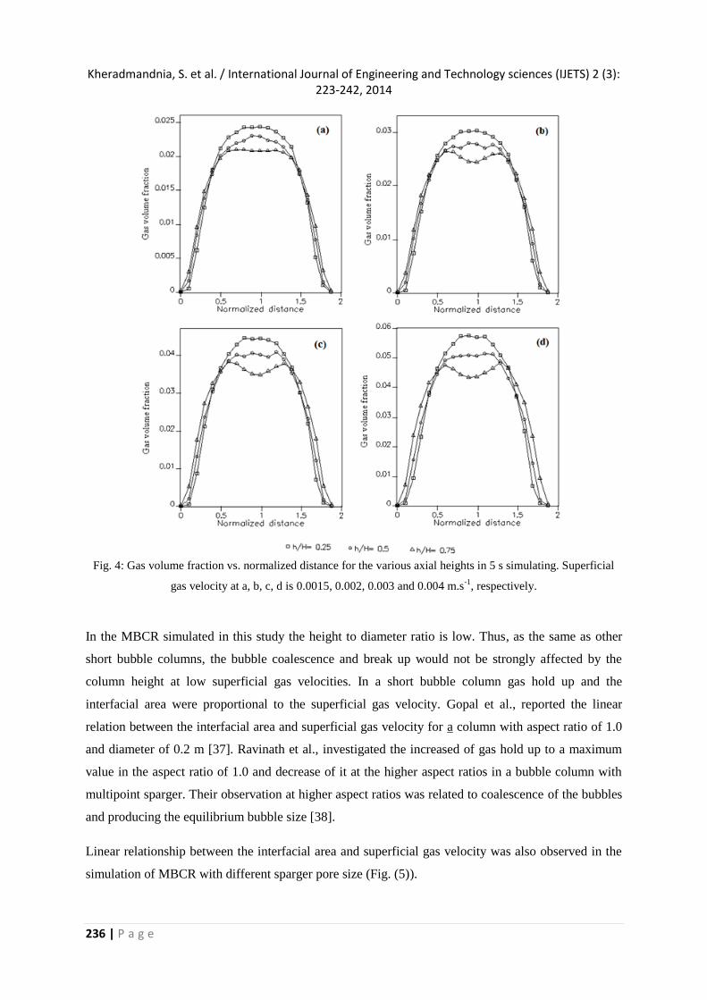
Linear relationship between the interfacial area and superficial gas velocity was also observed in the
simulation of MBCR with different sparger pore size (Fig. (5)).
Kheradmandnia, S. et al. / International Journal of Engineering and Technology sciences (IJETS) 2 (3): 223-242, 2014
237 | P a g e
Fig. 5: Linear relation between interfacial area and superficial gas velocity for different sparger pore sizes.
3.5. The effect of sparger pore size on the liquid velocity and the gas hold up
According to the literature, the multipoint sparger obtains higher gas hold up rather than single nozzle
gas spargers [17, 39, 40]. Higher value of gas hold up and interfacial area were obtained in the column
with the uniform sparged gas at the bottom. In a tall and large bubble column, type and design of the
gas sparger is not critical in the turbulent flow [6, 37]. But in a short bubble column gas sparger
design significantly affects the performance of the column [8, 38]. Sintered glass sparger with
different pore size used in this study to simulate the liquid circulation and gas hold up profiles in the
MBCR.
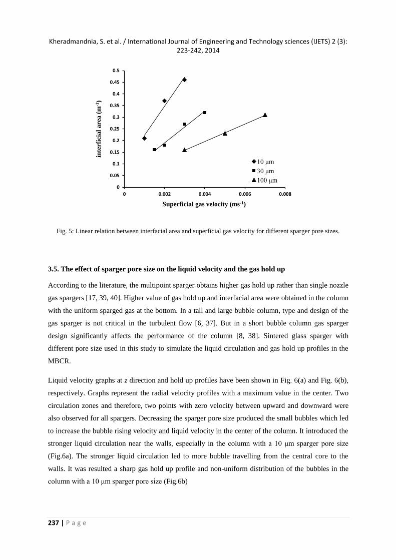
Liquid velocity graphs at z direction and hold up profiles have been shown in Fig. 6(a) and Fig. 6(b),
respectively. Graphs represent the radial velocity profiles with a maximum value in the center. Two
circulation zones and therefore, two points with zero velocity between upward and downward were
also observed for all spargers. Decreasing the sparger pore size produced the small bubbles which led
to increase the bubble rising velocity and liquid velocity in the center of the column. It introduced the
stronger liquid circulation near the walls, especially in the column with a 10 μm sparger pore size
(Fig.6a). The stronger liquid circulation led to more bubble travelling from the central core to the
walls. It was resulted a sharp gas hold up profile and non-uniform distribution of the bubbles in the
column with a 10 μm sparger pore size (Fig.6b)
0
0.05
0.1
0.15
0.2
0.25
0.3
0.35
0.4
0.45
0.5
0 0.002 0.004 0.006 0.008
inte
rfic
ial
are
a (
m-1
)
Superficial gas velocity (ms-1)
10 μm
30 μm
100 μm
Kheradmandnia, S. et al. / International Journal of Engineering and Technology sciences (IJETS) 2 (3): 223-242, 2014
238 | P a g e
Fig. 6: a) Liquid z- velocity graphs at different pore sizes of spargers; b) Gas volume fraction profiles at
different pore sizes of spargers. All graphs were obtained at the central x-z plane, superficial gas velocity of
0.003 m.s-1
and 5 s simulating.
By decreasing the sparger pore size, more number of the small bubbles entered in the column at a
defined velocity and the volume fraction of gas increased subsequently. It was resulted in increased
LK a . In the column with smaller pore size of the sparger. The values of average bubble diameter,
bubble rising velocity, gas hold up and LK a for different spargers at the superficial gas velocity of
0.003 m.s-1
have been shown in Table 2.
Table 2: Average bubble diameter, bubble rising velocity, gas hold up and LK a values for different sparger
pore sizes.
Sparger pore size (μm) bd
(1)(×10
-3m)
bu(2)
(m.s-1
) G LK a(3)
(s-1
)
100 0.81 0.43 0.021 0.033
30 0.61 0.48 0.027 0.069
10 0.42 0.58 0.032 0.13 (1)
bd is the average amount of bubble diameter calculated from equations (15) and (16) (2)
bu
is calculated from equation (14) (3)
LK a is predicted by CFD simulations according to equations (20) and (21).
3.6. Validation of the model
To prove the validity of the model, LK a was compared with the experimental data presented by Doig
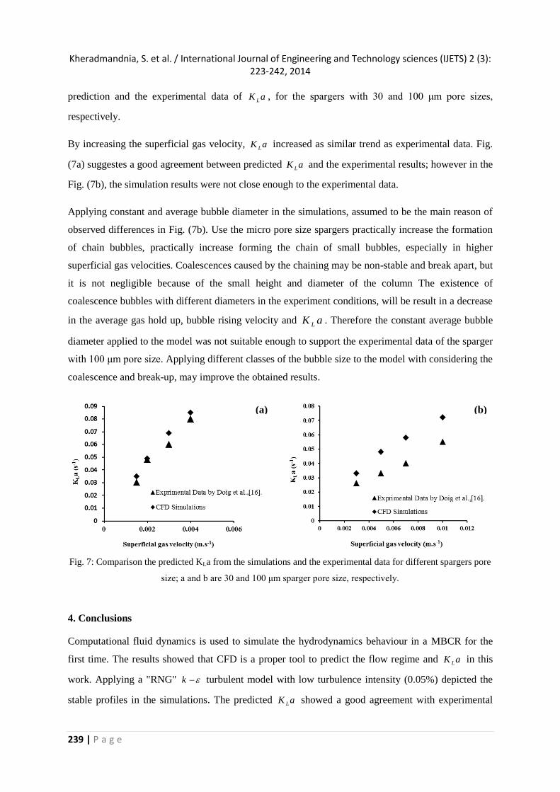
et al., [16] at different superficial gas velocities. Fig. (7a-b), shows a comparison between the model
Kheradmandnia, S. et al. / International Journal of Engineering and Technology sciences (IJETS) 2 (3): 223-242, 2014
239 | P a g e
prediction and the experimental data of LK a , for the spargers with 30 and 100 μm pore sizes,
respectively.
By increasing the superficial gas velocity, LK a increased as similar trend as experimental data. Fig.
(7a) suggestes a good agreement between predicted LK a and the experimental results; however in the
Fig. (7b), the simulation results were not close enough to the experimental data.
Applying constant and average bubble diameter in the simulations, assumed to be the main reason of
observed differences in Fig. (7b). Use the micro pore size spargers practically increase the formation
of chain bubbles, practically increase forming the chain of small bubbles, especially in higher
superficial gas velocities. Coalescences caused by the chaining may be non-stable and break apart, but
it is not negligible because of the small height and diameter of the column The existence of
coalescence bubbles with different diameters in the experiment conditions, will be result in a decrease
in the average gas hold up, bubble rising velocity and LK a . Therefore the constant average bubble
diameter applied to the model was not suitable enough to support the experimental data of the sparger
with 100 μm pore size. Applying different classes of the bubble size to the model with considering the
coalescence and break-up, may improve the obtained results.
Fig. 7: Comparison the predicted KLa from the simulations and the experimental data for different spargers pore
size; a and b are 30 and 100 μm sparger pore size, respectively.
4. Conclusions
Computational fluid dynamics is used to simulate the hydrodynamics behaviour in a MBCR for the
first time. The results showed that CFD is a proper tool to predict the flow regime and LK a in this
work. Applying a "RNG" k turbulent model with low turbulence intensity (0.05%) depicted the
stable profiles in the simulations. The predicted LK a showed a good agreement with experimental
(a)
(a)
(a)
(b)
Kheradmandnia, S. et al. / International Journal of Engineering and Technology sciences (IJETS) 2 (3): 223-242, 2014
240 | P a g e
data presented by Doig et al., [16] for the column with a 30 μm sparger pore size in this work. Liquid
circulation, gas distribution and their relation in the MBCR were as the same as the short bubble
columns with an aspect ratio lower than 1.0. Observation the similar trend in the hydrodynamic
characteristics of traditional and miniature scales of the bubble columns can encourage the researchers
to design the miniature bioreactors besides the lab scales and develop the industrial bioprocesses
using high-throughput systems.
Acknowledgments
The authors gratefully acknowledge the financial support of Biotechnology Development Council of
Islamic Republic of Iran (project Number: TMU88-8-66).
References
[1] Islam RS, Tisi D, Levy MS, Lye GJ. Scale-up of Escherichia coli growth and recombinant protein
expression conditions from microwell to laboratory and pilot scale based on matched kLa.
Biotechnology and Bioengineering. 2008;99:1128-39.
[2] Kostov Y, Harms P, Randers-Eichhorn L, Rao G. Low-cost microbioreactor for high-throughput
bioprocessing. Biotechnology and Bioengineering. 2001;72:346-52.
[3] Funke M, Diederichs S, Kensy F, Müller C, Büchs J. The baffled microtiter plate: Increased
oxygen transfer and improved online monitoring in small scale fermentations. Biotechnology and
Bioengineering. 2009;103:1118-28.
[4] Doig SD, Diep A, Baganz F. Characterisation of a novel miniaturised bubble column bioreactor
for high throughput cell cultivation. Biochemical Engineering Journal. 2005;23:97-105.
[5] Merchuk JC, Ben-Zvi S, Niranjan K. Why use bubble-column bioreactors? Trends in
Biotechnology. 1994;12:501-11.
[6] Kantarci N, Borak F, Ulgen KO. Bubble column reactors. Process Biochemistry. 2005;40:2263-
83.
[7] Betts JI, Baganz F. Miniature bioreactors: Current practices and future opportunities. Microbial
Cell Factories. 2006;5:21-35.
[8] Dhotre MT, Ekambara K, Joshi JB. CFD simulation of sparger design and height to diameter ratio
on gas hold-up profiles in bubble column reactors. Experimental Thermal and Fluid Science.
2004;28:407-21.
[9] Olmos E, Gentric C, Vial C, Wild G, Midoux N. Numerical simulation of multiphase flow in
bubble column reactors. Influence of bubble coalescence and break-up. Chemical Engineering
Science. 2001;56:6359-65.
Kheradmandnia, S. et al. / International Journal of Engineering and Technology sciences (IJETS) 2 (3): 223-242, 2014
241 | P a g e
[10] Ekambara K, Dhotre MT, Joshi JB. CFD simulations of bubble column reactors: 1D, 2D and 3D
approach. Chemical Engineering Science. 2005;60:6733-46.
[11] Darmana D, Deen NG, Kuipers JAM. Detailed modeling of hydrodynamics, mass transfer and
chemical reactions in a bubble column using a discrete bubble model. Chemical Engineering Science.
2005;60:3383-404.
[12] Dhaouadi H, Poncin S, Hornut JM, Midoux N. Gas-liquid mass transfer in bubble column
reactor: Analytical solution and experimental confirmation. Chemical Engineering and Processing:
Process Intensification. 2008;47:548-56.
[13] Lamping SR, Zhang H, Allen B, Ayazi Shamlou P. Design ofa prototype miniature bioreactor for
high throughput automated bioprocessing. Chemical Engineering Science. 2003;57:747-58.
[14] Zhang H, Lamping SR, Pickering SCR, Lye GJ, Shamlou PA. Engineering characterisation of a
single well from 24-well and 96-well microtitre plates. Biochemical Engineering Journal.
2008;40:138-49.
[15] Rihani R, Guerri O, Legrand J. Three dimensional CFD simulations of gas-liquid flow in milli
torus reactor without agitation. Chemical Engineering and Processing: Process Intensification.
2011;50:369-76.
[16] Doig SD, Ortiz-Ochoa K, Ward JM, Baganz F. Characterization of oxygen transfer in miniature
and lab-scale bubble column bioreactors and comparison of microbial growth performance based on
constant kLa. Biotechnology Progress. 2005;21:1175-82.
[17] Li G, Yang X, Dai G. CFD simulation of effects of the configuration of gas distributors on gas-
liquid flow and mixing in a bubble column. Chemical Engineering Science. 2009;64:5104-16.
[18] Zhang T, Wei C, Feng C, Zhu J. A novel airlift reactor enhanced by funnel internals and
hydrodynamics prediction by the CFD method. Bioresource Technology. 2012;104:600-7.
[19] Doran PM. Bioprocess engineering principles. first ed. London: Academic press; 1995.
[20] Krishna R, van Baten JM. Mass transfer in bubble columns. Catalysis Today. 2003;79-80:67-75.
[21] Monahan SM, Vitankar VS, Fox RO. CFD predictions for flow-regime transitions in bubble
columns. AIChE Journal. 2005;51:1897-923.
[22] Bhavaraju SM, Russell TWF, Blanch HW. The design of gas sparged devices for viscous liquid
systems. AIChE Journal. 1978;24:454-66.
[23] Sokolichin A, Eigenberger G. Applicability of the standard k-ε turbulence model to the dynamic
simulation of bubble columns: Part I. Detailed numerical simulations. Chemical Engineering Science.
1999;54:2273-84.
[24] Yakhot V, Orszag SA, Thangam S, Gatski TB, Speziale CG. Development of turbulence models
for shear flows by a double expansion technique. Physics of Fluids A. 1992;4:1510-21.
[25] Fluent A. Fluent 6.3 Users Guide. Fluent Inc. 2006.
Kheradmandnia, S. et al. / International Journal of Engineering and Technology sciences (IJETS) 2 (3): 223-242, 2014
242 | P a g e
[26] Ruzicka MC, Zahradník J, Drahoš J, Thomas NH. Homogeneous-heterogeneous regime
transition in bubble columns. Chemical Engineering Science. 2001;56:4609-26.
[27] Sokolichin A, Eigenberger G, Lapin A, Lṻbert A. Dynamic numerical simulation of gas-liquid
two-phase flows Euler/Euler versus Euler/Lagrange. Chemical Engineering Science. 1997;52:611-26.
[28] Delnoij E, Kuipers JAM, van Swaaij WPM. Computational fluid dynamics applied to gas-liquid
contactors. Chemical Engineering Science. 1997;52:3623-38.
[29] Mudde RF, Simonin O. Two- and three-dimensional simulations of a bubble plume using a two-
fluid model. Chemical Engineering Science. 1999;54:5061-9.
[30] Krishna R, van Baten JM. Eulerian simulations of bubble columns operating at elevated
pressures in the churn turbulent flow regime. Chemical Engineering Science. 2001;56:6249-58.
[31] Sokolichin A, Eigenberger G, Lapin A. Simulation of buoyancy driven bubbly flow: Established
simplifications and open questions. AIChE Journal. 2004;50:24-45.
[32] Delnoij E, Lammers FA, Kuipers JAM, van Swaaij WPM. Dynamic simulation of dispersed gas-
liquid two-phase flow using a discrete bubble model. Chemical Engineering Science. 1997;52:1429-
58.
[33] Silva MK, d’Ávila MA, Mori M. Study of the interfacial forces and turbulence models in a
bubble column. Computers and Chemical Engineering. 2012;44:34-44.
[34] Delnoij E, Kuipers JAM, van Swaaij WPM. Dynamic simulation of gas-liquid two-phase flow:
effect of column aspect ratio on the flow structure. Chemical Engineering Science. 1997;52:3759-72.
[35] Mousavi SM, Jafari A, Yaghmaei S, Vossoughi M, Turunen I. Experiments and CFD simulation
of ferrous biooxidation in a bubble column bioreactor. Computers & Chemical Engineering.
2008;32:1681-8.
[36] Wiemann D, Mewes D. Calculation of flow fields in two and three-phase bubble columns
considering mass transfer. Chemical Engineering Science. 2005;60:6085-93.
[37] Gopal JS, Sharma MM. Mass transfer characteristics of low H/D bubble columns. The Canadian
Journal of Chemical Engineering. 1983;61:517-26.
[38] Ravinath M, Kasat GR, Pandit AB. Mixing Time in a Short Bubble Column. The Canadian
Journal of Chemical Engineering. 2003;81:185-95.
[39] Bahadori F, Rahimi R. Simulations of Gas Distributors in the Design of Shallow Bubble Column
Reactors. Chemical Engineering & Technology. 2007;30:443-7.
[40] Buwa VV, Ranade VV. Dynamics of gas-liquid flow in a rectangular bubble column:
experiments and single/multi-group CFD simulations. Chemical Engineering Science. 2002;57:4715-
36.