modelling and evaluation of serial and parallel density

Faculty of Industrial Engineering, Mechanical Engineering andComputer Science

University of Iceland2019

Faculty of Industrial Engineering, Mechanical Engineering andComputer Science

University of Iceland2019

Modelling and Evaluation of Serialand Parallel Density-Based

Clustering for Acute RespiratoryDistress Syndrome

Chadi Barakat

MODELLING AND EVALUATION OF SERIALAND PARALLEL DENSITY-BASED

CLUSTERING FOR ACUTE RESPIRATORYDISTRESS SYNDROME

Chadi Barakat

60 ECTS thesis submitted in partial fulfillment of aMagister Scientiarum degree in Bioengineering

M.Sc. committeeDr. Sigurður Brynjólfsson

Dr. Morris Riedel

ExaminerDr. Helmut Wolfram Neukirchen

Faculty of Industrial Engineering, Mechanical Engineering and ComputerScience

School of Engineering and Natural SciencesUniversity of IcelandReykjavik, May 2019

Modelling and Evaluation of Serial and Parallel Density-Based Clustering for Acute Res-piratory Distress SyndromeClustering ARDS using Serial and Parallel DBSCAN60 ECTS thesis submitted in partial fulfillment of a M.Sc. degree in Bioengineering

Copyright c© 2019 Chadi BarakatAll rights reserved

Faculty of Industrial Engineering, Mechanical Engineering and Computer ScienceSchool of Engineering and Natural SciencesUniversity of IcelandTæknigarður - Dunhagi 5107, ReykjavikIceland

Telephone: 525 4700

Bibliographic information:Chadi Barakat, 2019, Modelling and Evaluation of Serial and Parallel Density-BasedClustering for Acute Respiratory Distress Syndrome, M.Sc. thesis, Faculty of IndustrialEngineering, Mechanical Engineering and Computer Science, University of Iceland.

Reykjavik, Iceland, May 2019

To my parents and my brothers for keeping me grounded,to my professors for pushing me forward,

and to my friends for reminding me to have fun along the way.

Abstract

Acute Respiratory Distress Syndrome (ARDS) is a highly heterogeneous conditionthat affects a relatively low number of mechanically-ventilated intensive care pa-tients, though its mortality rate is quite high, hence the need to develop early di-agnosis methods. In this thesis we developed, modelled, and evaluated an approachto extract patient data and evaluate it, perform pre-processing steps, and cluster itusing the density-based DBSCAN clustering algorithm. At the same time we madeuse of available High Performance Computing (HPC) technology in order to par-allelise the data manipulation processes. Our implementation showed a significantspeed-up in the performance of the highly compute- and data-intensive tasks whenusing the parallel computing infrastructure as opposed to running them in serial.Additionally, this process was used to assist in selecting the most effective values forthe clustering parameters. These results set the path for future implementations ofparallel computing in the large scale data extraction and analysis steps necessaryfor real-time diagnosis in a hospital environment. Furthermore, the pre-processingmethods developed in this thesis can easily be adapted to other conditions in theICU through the use of a HPC-ready Jupyter Notebook, which ultimately makesparallel computing accessible to clinicians without the need for expertise in parallelcomputing script development.

Útdráttur

Brátt andnauðarheilkenni er fjölþætt ástand sem hefur áhrif á tiltolulega fáa sjúk-linga í öndunarvél á gjörgæslu en hefur hins vegar háa dánartíðni, því er nauðsynað þróa snemmskimunaraðferðir. Í þessu verkefni var þróað og sett upp líkan, aðferðtil að sækja gögn sjúklinga ákvörðuð, forvinnsluskref framkvæmd og gögn þyrpuðeftir þéttleika með því að nota reikniritið DBSCAN. Einnig var notuð háafkastaútreikningatækni (e. High-Perfomance Computing (HPC)) til að samhliða reikninga.Útfærslun sýndi marktæka hraðaaukningu í afköstum útreikninga og meðferð gagnaþegar notaðir eru samhliða útreikningar miðað við raðbundnar keyrslur. Þetta ferlivar notað til að velja á gildi fyrir þyrpingar. Þessar niðursör leggja grunn að raun-tíma samhliða vinnslu á gagnagreiningu í umhverfi sem er á sjúkrahúsum. Ennfre-mur er hægt að aðlaga forvinnsluaðferðirnar í þessari rannsókn fyrir aðrar aðstæðurinnan gjörgæsludeilda með því að nota hugbúnaðinn Jupyter Notebook, sem gerirklínískum sérfræðingum kleift að nýta sér samhliða gagnagreiningu án þess að hafaþá sérfræðiþekkingu á samhliða gagnagreiningar kóða.

v

Contents

List of Figures ix

List of Tables xi

Abbreviations xv

Acknowledgments xvii

1. Introduction 11.1. Motivation . . . . . . . . . . . . . . . . . . . . . . . . . . . . . . . . . 11.2. Research Questions . . . . . . . . . . . . . . . . . . . . . . . . . . . . 21.3. Thesis Structure . . . . . . . . . . . . . . . . . . . . . . . . . . . . . . 2

2. Foundations 52.1. The MIMIC-III Database . . . . . . . . . . . . . . . . . . . . . . . . 52.2. Acute Respiratory Distress Syndrome . . . . . . . . . . . . . . . . . . 62.3. Unsupervised Learning and the DBSCAN Algorithm . . . . . . . . . 7

2.3.1. Unsupervised Learning . . . . . . . . . . . . . . . . . . . . . . 72.3.2. Principal Component Analysis . . . . . . . . . . . . . . . . . . 82.3.3. Clustering using DBSCAN . . . . . . . . . . . . . . . . . . . . 9

2.4. Parallel Computing and Clustering . . . . . . . . . . . . . . . . . . . 102.4.1. Parallel Computing and High Memory . . . . . . . . . . . . . 102.4.2. HPDBSCAN and Further Work . . . . . . . . . . . . . . . . . 11

3. Related Work 133.1. Clustering and Feature Analysis in the MIMIC Database . . . . . . . 133.2. Use of HPC Technology in ARDS Data Analysis and Clustering . . . 14

4. Data Analysis and Modelling Process 174.1. Business Understanding . . . . . . . . . . . . . . . . . . . . . . . . . 18

4.1.1. Business Objectives . . . . . . . . . . . . . . . . . . . . . . . . 184.1.2. Situation Assessment . . . . . . . . . . . . . . . . . . . . . . . 184.1.3. Goal Description . . . . . . . . . . . . . . . . . . . . . . . . . 204.1.4. Project Plan . . . . . . . . . . . . . . . . . . . . . . . . . . . . 21

4.2. Data Understanding . . . . . . . . . . . . . . . . . . . . . . . . . . . 224.2.1. Collecting Initial Data . . . . . . . . . . . . . . . . . . . . . . 22

vii

Contents

4.2.2. Data Description . . . . . . . . . . . . . . . . . . . . . . . . . 224.2.3. Data Exploration . . . . . . . . . . . . . . . . . . . . . . . . . 234.2.4. Verifying Data Quality . . . . . . . . . . . . . . . . . . . . . . 26

4.3. Data Preparation . . . . . . . . . . . . . . . . . . . . . . . . . . . . . 264.3.1. Dataset Description . . . . . . . . . . . . . . . . . . . . . . . . 264.3.2. Rationale for Data Selection . . . . . . . . . . . . . . . . . . . 274.3.3. Cleaning the Data . . . . . . . . . . . . . . . . . . . . . . . . 294.3.4. Constructing the Data . . . . . . . . . . . . . . . . . . . . . . 29

4.4. Modelling . . . . . . . . . . . . . . . . . . . . . . . . . . . . . . . . . 314.4.1. Selecting the Modelling Technique . . . . . . . . . . . . . . . . 314.4.2. Designing the Validation Process . . . . . . . . . . . . . . . . 324.4.3. Building the Model . . . . . . . . . . . . . . . . . . . . . . . . 324.4.4. Assessing the Model . . . . . . . . . . . . . . . . . . . . . . . 36

5. Evaluation 395.1. Experimental Setup . . . . . . . . . . . . . . . . . . . . . . . . . . . . 395.2. Evaluating Relevance of Data and Code Provisioning for ARDS . . . 405.3. Pre-processing and Clustering Result Evaluation . . . . . . . . . . . . 425.4. Gridsearch Result Evaluation . . . . . . . . . . . . . . . . . . . . . . 435.5. Review of Applied Processes . . . . . . . . . . . . . . . . . . . . . . . 43

6. Conclusion 47

References 48

Bibliography 49

A. Appendix 53

viii

List of Figures

2.1. Description of DBSCAN Clustering Parameters. . . . . . . . . . . . . 10

4.1. Overview of the modelling process. . . . . . . . . . . . . . . . . . . . 17

4.2. Number of admissions for an attributeID in the MIMIC database. . . 24

4.3. Number of patients for an attributeID in the Imputed Data. . . . . . 25

4.4. Number of patients for an attributeID in the reduced data. . . . . . . 28

4.5. Result changes at three steps of pre-processing. . . . . . . . . . . . . 30

4.6. Component analysis of the data. . . . . . . . . . . . . . . . . . . . . . 33

4.7. K-distance graph of the data. . . . . . . . . . . . . . . . . . . . . . . 35

5.1. Graphical depiction of attribute selection at the major steps of themodelling process and pre-processed data provisioning pipeline formedical users. . . . . . . . . . . . . . . . . . . . . . . . . . . . . . . . 41

5.2. Different possible combinations of minpts and epsilon and the numberof clusters produced . . . . . . . . . . . . . . . . . . . . . . . . . . . . 43

5.3. Four different clustering results with their respective parameters. . . . 45

5.4. ARDS patients as diagnosed using the Horowitz index. . . . . . . . . 46

ix

List of Tables

2.1. Selected information about the MIMIC-III database[1]. . . . . . . . . 6

5.1. Technical specifications of each of the servers in the JURON cluster[2]. 39

5.2. Technical specifications of the DEEP-ER SDV Prototype[3]. . . . . . 40

5.3. Time required to complete the pre-processing section of the code oneach type of architecture. . . . . . . . . . . . . . . . . . . . . . . . . . 42

xi

List of Code Snippets

4.1. Print number of patients for each attribute in MIMIC . . . . . . . . . 234.2. Extracting the number of patients from the imputed data represented

in each attribute. . . . . . . . . . . . . . . . . . . . . . . . . . . . . . 254.3. Selecting patients based on number of samples . . . . . . . . . . . . . 274.4. Reading imputed data and extracting the relevant features. . . . . . . 284.5. Initial pre-processing steps, revised below. . . . . . . . . . . . . . . . 294.6. Pre-processing the data by applying rolling average for smoothing

and standardising. . . . . . . . . . . . . . . . . . . . . . . . . . . . . 304.7. Diagnosing ARDS using the Horowitz index. . . . . . . . . . . . . . . 324.8. Determining principal components of the data based on information

content. . . . . . . . . . . . . . . . . . . . . . . . . . . . . . . . . . . 334.9. Applying PCA and computing the K-distance values. . . . . . . . . . 344.10. Applying the DBSCAN algorithm and saving the results to an output

file. . . . . . . . . . . . . . . . . . . . . . . . . . . . . . . . . . . . . . 344.11. Applying gridsearch in serial. . . . . . . . . . . . . . . . . . . . . . . 36

5.1. Writing diagnosis results in the output file. . . . . . . . . . . . . . . . 44

A.1. The code that was developed for this thesis. This code is only meantfor serial implementation. . . . . . . . . . . . . . . . . . . . . . . . . 53

xiii

Abbreviations

• AF - Atemfrequenz (breathing rate)

• ARDS - Acute Respiratory Distress Syndrome

• ASIC - Algorithmic Surveillance of ICU Patients

• CPU - Central Processing Unit

• CRISP-DM - Cross-Industry Standard Process for Data Mining

• csv - Comma-Separated Values

• DBSCAN - Density-Based Spatial Clustering of Applications with Noise

• DDR - Directly Density Reachable

• DEEP-ER - Dynamical Exascale Entry Platform - Extended Reach

• EHR - Electronic Health Record

• eps - Epsilon

• FiO2 - Fraction of Inspired Oxygen

• HF - Herzfrequenz (heart rate)

• HPC - High Performace Computing

• HPDBSCAN - Highly Parallel DBSCAN

• ICCA - IntelliSpace Critical Care and Anesthesia

• ICU - Intensive Care Unit

• ICD - International Statistical Classification of Diseases and Related Health

xv

List of Code Snippets

Problems

• JURON - JUelich neuRON

• MIMIC-III - Medical Information Mart for Intensive Care III

• minpts - Minimum Number of Points

• PaO2 - Partial Pressure of Arterial Oxygen

• PCA - Principal Component Analysis

• PEEP - Positive End-Expiratory Pressure

• Pplat - Plateau Pressure

• RWTH - Rheinisch-Westfaelische Technische Hochschule

• SMITH - Smart Medical Information Technology for Healthcare

• SQL - Structure Query Language

• Vt - Tidal Volume

xvi

Acknowledgments

I would like to express my deepest gratitude to everyone who has been a part of myexperience during these two years working towards achieving my Masters Degree atthe University of Iceland, but most notably Prof. Sigurður Brynjólfsson and Prof.Dr.-Ing. Morris Riedel for their constant support, follow-up, and guidance. Mythanks also go to every Professor and Instructor with whom I have taken courses,and the staff of the School of Engineering and Natural Sciences.

Additionally, I would like to thank Prof. Dr. med. Gernot Marx and Prof. Dr. rer.nat. Andreas Schuppert for their assistance at Uniklinik-RWTH Aachen and as partof the Joint Research Centre for Computational Biomedicine respectively, as well asmembers of staff in both institutions, most notably Oliver Maassen, Richard Polzin,and Konstantin Sharafutdinov.

Finally, my thanks go to the staff at Forschungszentrum Juelich for providing mewith access to the JURON and DEEP-ER SDV clusters in order to complete myresearch, and specifically to Dr. Gabriele Cavallaro and Rocco Sedona for theirassistance along the way.

xvii

1. Introduction

1.1. Motivation

In the statement of the rationale for the Algorithmic Surveillance of ICU patients(ASIC) use case, which is part of the Smart Medical Information Technology forHealthcare (SMITH) consortium [4], the researchers claim that around two millionpatients are currently being treated at Intensive Care Units (ICUs) around Germanyand that number will only increase in the coming years [4]. It is safe to assumethat this information is somewhat applicable around the world, and will thus posenew challenges that the medical community will have to overcome in order to keepproviding effective healthcare. For this reason, and since the advent of ElectronicHealth Records (EHRs) [5], much research has been done towards the integration oftechnology in the analysis of patients’ medical data in order to assist in forecasting,prevention, diagnosis, and treatment [5–11].

This thesis offers an approach to extract, process, and cluster patient medical infor-mation which highlights the benefits of applying advanced computing technologiesfor the service of healthcare research and industry. In essence, this master thesis in-vestigates the use of parallel and High Performance Computing (HPC) technology toread information from the Medical Information Mart for Intensive Care III (MIMIC-III) database [1], extract relevant information towards diagnosing Acute RespiratoryDistress Syndrome (ARDS) [12], perform pre-processing steps and dimensionalityreduction, and apply density-based clustering on the resulting data.

In order to perform these tasks, we (a) use state-of-the-art tools including an HPC-ready implementation of the Jupyter Notebook as a programming environment,which in itself is an immense advancement in terms of making HPC more accessi-ble and usable by clinical experts, (b) develop a pre-processing algorithm that canefficiently extract information from a medical database and can easily be adaptedto any medical condition given that the required parameters are known, and (c)perform a gridsearch that allows the visualisation of the most effective parametervalues for clustering the pre-processed data, thus performing an initial exploratorydata analysis while more elaborate models will be investigated in subsequent PhDstudies.

1

1. Introduction

Through this approach, we aim to highlight the significant speedup that can beachieved in data read-write processes by using parallel programming and HPC ar-chitecture. To properly structure the description of the modelling and evaluationprocesses involved in this research, we structure them based on the Cross-IndustryStandard Process for Data Mining (CRISP-DM) [13].

Finally, we use the Berlin definition [14] for ARDS diagnosis in order to develop atool that creates a list of the patients from the available pool that fulfill the criteriafor ARDS, which is then used to evaluate the clustering results.

1.2. Research Questions

In this thesis we discuss the background information acquired, the methods andapproaches implemented, the obstacles faced, and the solutions developed in theprocess of answering the following research questions:

• Can we develop methods to extract relevant data from the MIMIC-III database,label patient data, and pre-process them for ARDS research?

• Can we employ current HPC technology and different available HPC archi-tectures (JURON, DEEP-SDV) in order to accelerate the data pre-processingand clustering of large patient datasets while not losing sight of usability formedical experts?

• Can we investigate Density-Based clustering techniques on patient data ofARDS in the ICU as a first step of an exploratory data analysis?

1.3. Thesis Structure

This thesis is divided into six chapters as follows:

• Chapter 1 presents the general relevance of the research in question and intro-duces the research questions that we attempt to answer.

• Chapter 2 presents the background information and the fundamental conceptsupon which our research is based.

• Chapter 3 reviews related work in the field and discusses the current state of

2

1.3. Thesis Structure

affairs in terms of clustering applications and HPC use in ARDS research.

• Chapter 4 follows the initial phases of the CRISP-DM model by introducingthe tools that will be used and describes the model that was developed in orderanswer the research question from Chapter 1.

• Chapter 5 continues with further CRISP-DM phases and describes the exper-imental setup used to perform the modelling steps, discusses the results of ourmodelling, and evaluates them with respect to the available validation tools.

• Finally, Chapter 6 provides a summary of the work that was done and presentsthe future work that this research paves the way for.

3

2. Foundations

2.1. The MIMIC-III Database

Acquiring access to Electronic Health Records (EHRs) [5] of patients in the IntensiveCare Unit (ICU) is in most cases problematic as it raises concerns in terms of thepatients’ privacy. It is well established in the medical field that some information isshared among medical professionals to draw conclusions as to a specific condition,prepare a treatment plan, follow up on progress of the medical condition, and ifpossible gain new information from the changes in the patients’ state. It is howevernot always clear what extent of the data can be shared within the broader publicmedical sciences community, and what should be kept private. Similarly, dealingwith real-world data that is constantly being updated poses the risk of corrupting theinformation contained within and is not a viable option when it comes to analysingprocedures and their success rates. Hence, the MIMIC database was established andmade available to the medical community as a free-to-access resource comprising alarge population of ICU patients [1].

MIMIC-III (Medical Information Mart for Intensive Care III) is the third and mostrecent version of the database, containing data from around 40.000 patient ICUstays between 2001 and 2012 at the Beth Israel Deaconess Medical Center, BostonMA. The patient information contained within the database is deidentified and madeavailable freely to medical professionals and researchers, and has been used as thebasis for research in many publications dealing with respiratory conditions [9], sepsis[7][8], and computer-assisted diagnosis of the patient’s medical state [5].

Though access to the database is free, it is not fully open, but access is grantedonly to parties that have completed a course on the proper handling of medical andother such sensitive information, and who can provide a general direction in whichthe data will be employed as long as it is not for profit. In our case, the course wascompleted and access was granted based on proof of supervision as part of a MastersThesis and a description of the type of research that the data will be employed in.

The information is stored in the database as part of tables, describing much of thepatient’s stay in the hospital from admission (e.g. including time, date, religion, basis

5

2. Foundations

of admission, initial prognosis, International Statistical Classification of Diseasesand Related Health Problems (ICD) codes etc.) through ICU stay highlightingventilation parameters, physiological measurements, and blood gas and other suchanalysis data, and finally detailing discharge (whether to hospital, to home, or deathof the patient). The database, the size of which exceeds 40GB, is obtained from thePhysioNet servers in Structure Query Language (SQL) format, while manipulation ofthe data in our case was done using code that queries the dataset, extracts relevantinformation to the research questions presented above, processes it, and outputsresults as will be discussed in the further sections of this report.

Table 2.1: Selected information about the MIMIC-IIIdatabase[1].

Data collected between 2001 and 2012Beth Israel Deaconess Medical Center26 Tables> 40.000 PatientsAll Intensive Care Unit patients47GB Database size + 26GB for Indexes

2.2. Acute Respiratory Distress Syndrome

Acute Respiratory Distress Syndrome (ARDS) is a condition that affects mechani-cally ventilated patients in such a way that there is an observed increase in breathingrate, a drop in blood oxygen levels, a loss of lung compliance, and a presence of flu-ids in the alveoli [12] as first described by Ashbaugh et al. in 1967. At the time,it was noted that the patients exhibited similar symptoms to those observed ininfantile respiratory distress syndrome, while onset of the condition was generallypreceded either by severe trauma or viral infection. Additionally, the authors firstdescribed the condition due to the curious case that those affected would not re-spond to traditional respiratory therapies, while other treatments including PositiveEnd-Expiratory Pressure (PEEP) control and corticosteroid therapy were success-ful to some extent [12]. Since then, much research has been done on the natureof ARDS, its onset, prevalence, prevention, diagnosis, and treatment as will be de-scribed hereafter, though it remains a highly heterogeneous condition.

In their paper on the incidence and outcome of ARDS, Villar et al. analyse hospitaladmissions in several areas in Spain between 2008 and 2009 and highlight ARDSdiagnosis during this time interval [15]. Their findings highlight the low incidenceof ARDS in patients (7,2 cases per 100.000 patients) while it sheds light on the highmortality rate of this condition where it proved fatal in 42.7% of diagnosed ICU

6

2.3. Unsupervised Learning and the DBSCAN Algorithm

patients. Additionally, the heterogeneity of ARDS is obvious in the discussion ofthe paper’s results where the authors mention the existence of different criteria fordiagnosis of the condition depending on the location of the hospital.

To combat the confusion and uncertainty in defining ARDS, the Berlin Definition ofARDS was introduced in 2012 [14] which clearly defines the physiological parametersbased on which accurate diagnosis of patients can be made. The Berlin Definitionalso takes into consideration defining the severity of the condition based on thePEEP value as well as the ratio of the partial pressure of arterial oxygen PaO2 tothe fraction of inspired oxygen in the air FiO2 (i.e. the amount of oxygen suppliedin the mechanical ventilation airflow) as follows:

• Mild ARDS: 200 mmHg ≤ PaO2/FiO2 ≤ 300 mmHg, PEEP ≥ 5 cmH2O.

• Moderate ARDS: 100 mmHg ≤ PaO2/FiO2 ≤ 200 mmHg, PEEP ≥ 5 cmH2O.

• Severe ARDS: PaO2/FiO2 ≤ 100 mmHg, PEEP ≥ 5 cmH2O.

Even though since the implementation of the Berlin Definition the diagnosis ofARDS has been standardised in medical institutions, the condition remains at thecentre of extensive research due to the difficulty in treating it and the differentfactors that lead to its onset.

Furthermore, in-depth analyses of ARDS patient data have shown that even thoughthe condition is highly heterogeneous, two distinct phenotypes can be defined withone showing a lower mortality rate, while the other presents more severe inflam-mation. These findings were discussed in two separate papers by Bos et al. [16]and by Calfee et al [17]. In fact, Bos et al. define the subphenotypes as either "un-inflamed" or "reactive" which coincide with "phenotype 1" and "phenotype 2" asdefined by Calfee et al. These findings show that there are intricacies to this con-dition that physicians should take into consideration before deciding on the mosteffective treatment method.

2.3. Unsupervised Learning and the DBSCANAlgorithm

2.3.1. Unsupervised Learning

In machine learning applications, unsupervised learning is the process through whichrelevant information is obtained from a given dataset without any prior knowledge

7

2. Foundations

of the data itself, as opposed to supervised learning where the program is providedwith a learning set that allows it to draw features based on which future decisionswill be made [18]. In essence, the totality of the data is loaded into the learningapplication and, based on distance or similarity metrics, relevance and/or internalrelationships between the data points are highlighted.

Unsupervised Learning processes are often considered in the analysis of big data[18] and are used to get a better understanding of the data itself. Their potentialapplications are in clustering data, detecting outliers and noise, and reducing di-mensionality in order to simplify grouping and analysis of the dataset in question.From these processes we are mainly interested in dimensionality reduction whichwill be applied to large datasets such as those obtained from EHRs and clusteringwhich will link together points that are evaluated as being similar. The dimension-ality reduction techniques, as well as the potential clustering approaches that willbe discussed in the following section constitute part of the exploratory data analysisprocesses through which relevant information can be extracted from relatively noisydatasets [18].

Below we discuss one major dimensionality reduction technique, Principal Compo-nent Analysis (PCA) [18], then after introducing the feature engineering and selec-tion techniques with dimensionality reduction, we discuss the DBSCAN algorithm,a clustering method that uses distance and density to draw relevant informationfrom a given dataset.

2.3.2. Principal Component Analysis

Principal Component Analysis (PCA) is a commonly used method for dimensionalityreduction in high dimensional data. Before explaining the process of how PCA isapplied, we first need to introduce the concept of dimensionality reduction. As Shaiet al. explain it, dimensionality reduction is the process of taking a high dimensionaldataset and "mapping" it to a new space of lower dimensions which would make iteasier and less compute-intensive to analyse, graph, or comprehend [18].

PCA achieves the tasks described above by performing linear transformations on thedata in such a way that the variances of the original data with respect to the newspace are sorted in descending order. These variances are seen as vectors and eachrepresents one principal component of the data that represents a significant part ofthe whole. By analysing the information content of each vector we can determinehow many components we need so as to represent the original dataset in a lowerdimension, without too much loss of information.

8

2.3. Unsupervised Learning and the DBSCAN Algorithm

2.3.3. Clustering using DBSCAN

Choosing a specific approach to clustering a dataset often has a great effect on howthe results are interpreted in the end and therefore, it is essential to understand thedata being analysed as well as to know the specific means by which the clusteringalgorithm will find relevant features within the information. Knowing that medicaldata is rarely ever complete, especially given the fact that the information containedin the dataset selected in this research is of a relatively large size and extends over along duration, our selection of a clustering algorithm needs to take into considerationthe fact that noise constitutes a major part of the dataset, that missing values haveto be accounted for, and that the high dimensionality of the data might hinder theanalysis process.

Ester et al. [19] proposed in 1996 in their paper "A density-based algorithm fordiscovering clusters in large spatial databases with noise" a clustering approach thatfulfils most of the requirements described above. Their algorithm named DBSCAN(Density-Based Spatial Clustering for Applications with Noise) is one of the mostwidely used clustering methods that is currently still in use and has had manyvariations that have allowed it to adapt to a wide range of applications as will bediscussed below.

In contrast to other clustering techniques like K-means clustering [20], DBSCANalgorithm does not take into consideration a pre-defined number of clusters. Asshown in Figure 2.1, and in order to identify an arbitrary number of clusters, itrather defines each point as either a core, border, or noise point. This definition isdone by counting the number of datapoints within a radius ε around each point; ifthe number of samples including the point being considered is equal to or greaterthan a predefined minpts value (minimum number of points), then the point isconsidered a core point. The points within the ε radius are thus directly densityreachable (DDR) and belong to the same cluster. Points that do not achieve minpts,but are directly density reachable are considered to be border points and thus definethe borders of a cluster. Finally, data points that are not directly density reachableand do not achieve minpts are thus considered noise points.

As ε and minpts are the only parameters necessary for the application of the DB-SCAN algorithm, the process of selecting these values greatly affects the number,shape, and size of the obtained clusters. Accordingly, we choose minpts and ε basedon specific criteria which will be introduced in the Modelling and Evaluation chap-ters.

One of the major advantages of density-based clustering is the fact that non-globularclusters do not pose a challenge to the algorithm, as opposed to K-means and hier-archical clustering. The approach of defining core, border, and noise points allows

9

2. Foundations

Figure 2.1: Description of DBSCAN Clustering Parameters.

DBSCAN to discover clusters within clusters. Furthermore, DBSCAN specificallypresents the extra advantage of taking noise into consideration in its application,thus filtering the output results further and ultimately providing more precision interms of clustering.

On the other hand, DBSCAN presents some shortcomings when the densities of theclusters vary greatly, thus causing erroneous readings. Additionally, the resultingclusters greatly depend on the choice of ε and minpts which requires the researcherto verify their choice of parameters or otherwise risk obtaining incorrect results.In fact, the interpretation of results based on the use of different parameters forclustering needs to be evaluated by medical experts and as such can not be fullyperformed in this master thesis. Instead as the SMITH Project advances, feedbackwill be provided in order to enhance these results. Finally, DBSCAN is not effectivewhen it comes to clustering high-dimensional data which, especially in our case,would require a reduction in the dataset’s dimensionality, a step which, if the datais not well understood, might cause erroneous readings.

2.4. Parallel Computing and Clustering

2.4.1. Parallel Computing and High Memory

Despite the constant advancements in technology leading to the development ofcheaper, more efficient, and more powerful electronic components, Moore’s Law,which states that the number of transistors within a processor will double every twoyears, seems to be reaching a plateau at this time as the size of the componentsdraws closer to the atomic scale. This however, is countered by the implementationof parallel processing and High Performance Computing (HPC) technology which

10

2.4. Parallel Computing and Clustering

allow for a great amount of scaling and speed-up.

HPC is the concept of developing architectures that allow Central Processing Units(CPUs) to intercommunicate efficiently via high-performing interconnections, thuscompleting highly compute-intensive operations by dividing the workload. This ispossible through the use parallel computing which is a process by which severalcores/CPUs perform a given task in a cooperative manner [21]. Programming inparallel, in any language, is a challenging prospect as it requires the person to thinkin such a way as to make use of the available architecture and cores in the mostefficient manner. In this type of programming the maximum speed-up occurs whenthe load is balanced on all components. Among other things, this technology hasallowed the visualisation and simulation of extremely complex concepts such as fluidflows, both laminar and turbulent.

In this report we perform analyses on two HPC architectures of the Forschungszen-trum Juelich (FZ-Juelich) the properties of which are discussed in tables 5.1 and5.2 presented in Chapter 5. These supercomputers are JURON (JUelich neuRON)and the Dynamical Exascale Entry Platform - Extended Reach (DEEP-ER), and willprovide the platform over which data manipulation is performed in a semi-automatedfashion, as well as to assist in the selection of the most effective parameters for theclustering algorithm.

2.4.2. HPDBSCAN and Further Work

Knowing that applying DBSCAN clustering on a dataset as large as the MIMIC-IIIdatabase, which involves time series data for several attributes of tens of thousandsof patients, would be a heavy load for any basic computer, the rational next stepwould be to perform the required calculations using more advanced architecturesthan standard laptop or desktop PCs. Hence, we look into the research of Götz etal. [22] in their paper "HPDBSCAN - Highly parallel DBSCAN" which presents anapplication of the aforementioned clustering algorithm that is adapted to parallelcomputing architectures including scalable data infrastructure. In their paper, theresearchers describe their approach and compare it to other attempts at parallelisingthe DBSCAN algorithm, which comes down to three features: 1) reducing the totalworkload by splitting the tasks to be performed over the totality of the availablearchitecture, 2) preprocessing the data indices so that all parts of the data areknow by the system and every part can be traced and collected, and 3) a rule-based merging scheme for the created clusters whereby the clusters formed at eachnode can be linked together to define the final clustering scheme that was producedby the algorithm. They were able to show that HPDBSCAN presents sustainablescalability and speed-up with increasing size of a given dataset that was used forbenchmarking as opposed to another approach at DBSCAN parallelisation. At the

11

2. Foundations

time of writing, it appears to be the best parallel and scalable DBSCAN approachfor HPC systems and is therefore picked in this thesis as one potential tool for dataanalysis.

12

3. Related Work

3.1. Clustering and Feature Analysis in the MIMICDatabase

As described in the Foundations chapter, the MIMIC-III database is a treasure troveof information for biomedical researchers given that it deals almost exclusively withcritically ill patients and contains a large amount of medical parameters, physiologi-cal signals, and waveforms. For this reason much research has been done on clinicalconditions that occur in the ICU by analysing the data contained within the MIMICdatabase and drawing conclusions from the observed patterns. In this section wewill consider two such approaches, one attempting to map patient trajectories usingdeep learning while the other deals with sepsis, and then discuss other work dealingwith the computational processing of MIMIC and other EHR data. Hence, to thebest of our knowledge, no published work on clustering with feature analysis onARDS has been done.

Beaulieu-Jones et al. [5] implemented deep learning techniques on patient data ex-tracted from the MIMIC database and were able to develop an algorithm that pre-dicts patient state evolution and response to the healthcare being provided. In theirapproach, they applied autoencoders to reduce the dimensionality of the data andto group them into clusters. This data would then be analysed in a unsupervisedmanner (and evaluated using supervised learning techniques) to predict possibleoutcomes for the patient and select the most likely. No specific condition was anal-ysed for this approach, though the authors refer to potential applications in chronicdiseases such as type 2 diabetes.

Ghalati et al. [7] considered phase transition in their research on sepsis, focusingmainly on the warning signs that highlight the impending shift in a patients statefrom chronic to acute. Their approach required the implementation of machinelearning techniques such as support vector machines and logistic regression as well asa new concept of surprise loss to analyse the data and differentiate non-sepsis patientfrom those developing septic shock, while also highlighting the markers leading tothe tipping point so as to signal disease onset.

13

3. Related Work

In their research, Afshar et al. [10] applied Natural Language Processing (NLP) andMachine Learning (ML) techniques on the medical records of burn and trauma ICUadmissions in order to diagnose ARDS. Their approach provided diagnosis with anaccuracy of 83% as opposed to 67.3% for the traditional approach of determiningthe PaO2/FiO2 ratio and PEEP at 7 days after the onset of lung injury.

Similarly, Huddar et al. [9] showed the potential effectiveness of analysing clinicalnotes in assisting diagnosis of critical respiratory failure. Their research takes intoconsideration an earlier version of the MIMIC database, and extracts from it featuresthat indicate the onset of post operative respiratory failure well before it is diagnosedby the clinicians involved.

Komorowski et al. [8] implemented machine learning techniques, namely reinforce-ment learning to create a computational model that is able to diagnose sepsis andsuggest treatment strategies in order to curb the progression of the condition. Theirresearch shows the potential that such machine learning and automated data anal-ysis techniques have as diagnosis tools as they are able to detect patterns in largescale data that would otherwise go unnoticed by a human observer.

3.2. Use of HPC Technology in ARDS DataAnalysis and Clustering

While reviewing related work and publications regarding ARDS and HPC, we foundthat, regardless of the research done on both of these concepts separately, little tono work has been done on combining them. However, we did find a paper that,instead of analysing or clustering ARDS data, attempts to model it in a simulationenvironment on HPC. The paper by Das et al. [11] describes the development of amodel that simulates the effects that ARDS has on cardiovascular and pulmonarysystems of patients. Their model, which runs on HPC systems at the Universityof Warwick, takes for input patient data and implements it in such a way as tobe able to respond to changes in the environment where the researchers were ableto highlight similarities between the outputs of the virtual patient and the clinicaltrials.

This work defines the potential applications that HPC has in ARDS research as itprovides an efficient platform over which to develop simulations that could eitherbe used to train physicians or adapted to predict the direction in which a patient’shealth state is evolving.

On the other hand, the available literature does present a growing interest in HPC

14

3.2. Use of HPC Technology in ARDS Data Analysis and Clustering

applications in healthcare as can be seen in the workshop report on "High Perfor-mance Computing in Health Research", detailing the discussions and outcomes ofthe workshop organised by the European Commission in Brussels in October of 2014[6]. In this report we can highlight the trend towards encouraging the developmentof HPC in the European Union, as well as the growing market for this technologyin healthcare applications, mainly in drug development and health research.

15

4. Data Analysis and ModellingProcess

After introducing the basic concepts that govern the work presented in this thesis,and describing research that attempts similar approaches or deals with similar med-ical conditions, we move towards describing the work that we set out to achieve inour study. The process by which the data is selected, manipulated, and analyseddescribed in this chapter, as well as the evaluations steps in the following chapterare organised and presented following the Cross-Industry Standard Process for DataMining (CRISP-DM) [13]. The major steps of this process are laid out in Figure 4.1presented below.

Figure 4.1: Overview of the modelling process.

17

4. Data Analysis and Modelling Process

4.1. Business Understanding

4.1.1. Business Objectives

As discussed in Chapter 2, ARDS is a highly heterogeneous condition that affects asignificant number of mechanically ventilated ICU patients and has a high morbidityand mortality rate (42.7% [15]). Treatment methods of ARDS vary in effectivenessdepending on their implementation period, and therefore early detection and warn-ing systems would be an invaluable tool in combating this condition.

The business objectives of this thesis, as defined by the research questions presentedin Chapter 1, are to develop a system that can analyse an input set of ICU patientinformation, uncover underlying interactions and connections, and cluster the datain an unsupervised manner which will allow us to identify subgroups of patients thatmay develop ARDS.

In the process of achieving the objectives described above, we provide a tried-and-tested method of data manipulation in terms of pre- and post-processing, analysis,and storage, both in a serial and parallel environment, that will be freely accessibleby colleagues in the Algorithmic Surveillance of ICU Patients (ASIC) use case ofthe SMITH project in specific, as well as future researchers in this field in general.In terms of the specific clustering results obtained using our method, namely DB-SCAN, the analysis method used is a novel approach and the parallelisation of thework paves the way for new methods for dealing with compute- and data-intensiveanalyses of medical information. It goes without saying that objectives with respectto the clear interpretation of clustering results and further predictive models requiremedical know-how and is as such out of scope of this master thesis.

4.1.2. Situation Assessment

Inventory of Resources

For the purpose of completing the tasks defined in our research objectives we em-ploy an extensive set of resources and tools; these include the database itself, theprogramming language used to analyse it and the modules it employs in order toperform the tasks, and finally the platforms, both hardware and software, over whichthe process is done. What follows is a description of these tools.

The MIMIC-III database is available for download from the Physionet servers for

18


confirmed and approved research purposes as was described in the foundations sec-tion in more detail. After approval, querying the data is done using a SQL connectionvia the programming software being used. In our case, all programming was donein Python running on a Jupyter Notebook [23], with the scikit-learn, feather, pan-das, numpy, matplotlib, and mpi4py modules installed. These modules are mainlyadapted for analysis, lightweight storage, data manipulation and read-write pro-cesses, array operations, and data visualisation respectively.

Keeping in mind the size of the database (upwards of 40GB), the platform overwhich the work is done is of great importance as storage capacity and memory willultimately affect performance. For this reason, the analysis is first performed locallyon a personal computer in order to provide a benchmark representing serial workingenvironments and illustrating their shortcomings. The local machine is a MacBookPro (2015) with a 2,7 GHz Intel Core i5 processor, 250GB of internal SSD storagecapacity, and 8GB of 1867 MHz DDR3 RAM.

Another resource that will be used in the remainder of the data analysis is the JU-RON cluster of the Jülich Supercomputing Centre, which is a pilot system developedby IBM and NVIDIA, and the DEEP-ER SDV cluster, which is a prototype clusterdeveloped as part of the DEEPprojects, a collaborative research project funded bythe European commission. JURON is made up of 18 servers, while the DEEP-ERcluster has 16 nodes and a booster of 8 CPUs. The specifications of both HPCclusters are presented in Tables 5.1 and 5.2 provided in Chapter 5.

Constraints

In terms of data use, manipulation, and distribution, a lot of the work done inthis project involves dealing with information that is either meant for personal useor completely confidential. Certainly this would pose several risks which will bediscussed below, however the restrictions on the data also put limitations as to howit can be used. In essence, though the MIMIC database is open, access to it is limitedto research purposes that have been approved by the providers, and accordingly isnot meant for distribution. Thus, the results of the research being performed canbe discussed, though special care must be placed in the process so that none of theoriginal data is divulged.

Similarly, analysis that was performed by the Bayer pharmaceutical group resulted ina list of subjects from the database that were confirmed ARDS patients, which wouldgreatly simplify the validation and evaluation of the clustering results. However,since their research has not been made public and is completely confidential, itcannot be used in this master thesis, but is available for further research in the jointSMITH project.

19


Risks and Contingencies

In terms of risks involved in the process of answering the research questions listedabove, the analysis being performed is expected to not lead to divulging any infor-mation that is determined to be confidential or for internal use. The data obtainedfrom Bayer cannot reasonably be used without risk of it being inferred from theresults and is thus dropped from analysis.

On the other hand, information is freely transferred between the partners in theASIC use case for the purpose of advancing the project towards fruition, howeverit is not yet published and should thus not be made public in any way that mayundermine the work being done. In the same scope, the work that is describedin this thesis will ultimately benefit the partners in this project in terms of thedata manipulation that was performed, the programming that was done, and thehardware that was employed. On the larger scale, other potential researchers in thediagnosis and treatment of ARDS will benefit from this research after the publicationof our approach and results. By taking care of leaving sensitive material out anddiscussing with project partners, it is clear that the Master Thesis can be publishedas is.

4.1.3. Goal Description

While attempting to uncover features and signs that pinpoint the onset of ARDSin the patient data is our ultimate goal, we first need to understand the data itself.This becomes mostly clear when we are faced with the large amount of informationthat every individual patient ID is associated with in terms of admission notes,vital signs, drug supply, nursing and doctor’s notes, ICD codes, etc. Hence, it isessential to perform a significant amount of data reduction and manipulation beforeeven attempting to consider the individual patients themselves. Afterwards, furtheranalysis and reduction is applied to the dataset that will result in data that canbe clustered in a meaningful manner. This process of navigating the database,highlighting the relevant information, collecting, cleaning, and analysing it, andfinally storing it in easily accessible files for clustering is in itself one of the ultimategoals of this research. The reason for this inclusion is to simplify the preliminarywork that future researchers in this area will have to perform by providing a roadmap for adapting MIMIC-III data so that it can be used in ARDS research.

In parallel, the goal of unsupervised learning in general is to underline features withina given dataset that would imply correlation, causality, or similarity, which wouldnot be immediately apparent. This goal is mirrored in our approach of cluster-then-predict where we intend to highlight inherent differences between ICU patients that

20


would ultimately lead some of them to develop ARDS, as well as between subclassesof ARDS patients as was discussed in the papers by Bos et al. and Calfee et al.Another goal is to use High Performance Computing (HPC) to speed-up the dataanalysis process and to provide access for medical experts in a seamless fashion (e.g.using Jupyter Notebook instead of SSH Connections). This is needed since medicalexperts require access to the clustering tool, but are not technical experts to performSSH-key based access or to use scheduling principles of HPC machines.

4.1.4. Project Plan

In attempting to answer the research questions proposed in the introduction of thisthesis report, we employ several tools and techniques as described above that willassist in the development of our problem solving approach. The choice of these toolsis described hereafter, though it is mainly based on the current state of the art interms of technology, trends in programming, and in some cases, necessity.

In first place, performing our analysis on the MIMIC-III database is an essentialpart of the project and is based on its ready availability for research such as ours.Logistically speaking, working with a team from the Uniklinikum Aachen, we wouldhave been able to request access to the IntelliSpace Critical Care and Anesthesia(ICCA) database [24], however it is significantly smaller than the MIMIC dataset,is proprietary, confidential, and only accessible to faculty and staff of the Universityof Aachen.

Second, and given our understanding of the data, we know that the samples areinherently noisy, numerous, and high-dimensional. The choice of DBSCAN, analgorithm having noise reduction and outlier detection as a major part of its appli-cation, with confirmed uses on large scale datasets [25], for clustering the data isthus explained.

Third, employing Python in all phases of project development, from pre- to post-processing, passing through clustering, is based on this specific programming lan-guage’s extensive relevant literature, modularity, and widespread implementation inmachine learning applications. It is a relatively easy language to learn and apply,and the add-on modules available make it a sturdy tool for use in data manipulationand unsupervised learning approaches as the ones described in this report.

Finally, and given the data- and compute-intensive nature of the application inquestion, we seek out the substantial speed-up and storage that can only be achievedusing parallel computing architectures. Though the database and all processingwas initially performed on a local machine, loading the data onto the clusters andimplementing parallelisation of the program presented larger capacity for file storage

21


and scale-up. The benefit of scale- and speed-up however should not come at thecost of usability for medical expert users and as a consequence, Jupyter Notebookis planned as a compromise between technical difficulty and usability.

4.2. Data Understanding

4.2.1. Collecting Initial Data

After completing a required course on the ethical handling of patient data andobtaining access to the MIMIC database, it can be cloned onto a local machine andread via a SQL database management software as described in the extensive tutorialposted on the Physionet website. In our case, we obtained access to the RWTH-Aachen University servers which contain a copy of the database (thus eliminatingthe need to store it locally) and can be accessed using a Python code. By calling thefunction getCnx() defined in this code, and naming the specific required table (fromthe list presented in the Foundations section), we can load patient information intoa Pandas dataframe [26] for analysis.

The tables that were loaded are “chartevents” and “labevents” as they hold theattributes most closely related to the research we are performing. The obtaineddataframe consisted of approximately 45.000 unique patient IDs. It is worth notingat this point that these patients have all been admitted to the ICU but, given thatwe are only interested in mechanically ventilated patients as the population mostlikely to develop ARDS, further data reduction is necessary.

The reduction was done by project partners from the University of Aachen who wereable to select only the mechanically ventilated patients from the list and presentthem as individual files in .feather format [27]. The number of patients was thusreduced to 24.918 while some data manipulation was performed on the attributesand the values contained within each file.

4.2.2. Data Description

The data that is loaded from the MIMIC database is a time series data that hasmany attribute IDs, several of which represent the same measured value. This ismade obvious in the figures presented below in our exploration of the data, thoughin this section it is mentioned in order to justify the data imputation that wasperformed. A sample of the attributes is presented in Chapter 5.

22


The imputed data that was received from our partners at Aachen University, be-sides having a smaller number of patients (having only selected the ones undergoingmechanical ventilation), also has a smaller number of attributes, a more consistenttimestamp, and no missing values beyond the first recorded value for each attribute,i.e. the only “NaN” values present in the data are either at the start of the signal, orin completely empty attributes. In total, each patient has a “charttime” attributewhich is the timestamp value in 30 minute increments beginning at admission andending at either discharge or death, followed by 44 attributes listing different vitalsigns including, but not limited to, heart rate, breathing rate, tidal volume, bloodpH, breathing parameters, blood gas analysis results, and blood test results. Eachpatient’s information is saved in a feather format file with title including the uniquepatient ID. Though this step reduced the overall size of the dataset, it was stillsomewhat bulky, taking up a total of 5,3GB of space.

4.2.3. Data Exploration

In this section we describe the attributes present in the dataset at the three ma-jor steps before we begin our main pre-processing phase. These steps are (1) thecomplete MIMIC dataset, (2) the imputed data obtained from our partners, and (3)after selection of the most relevant attributes to our research.

What follows is a visualisation of the number of patients who have data recorded fora given attribute in the datasets. The first graph presents the results obtained whenquerying the MIMIC database, and it clearly shows the large number of attributesand patients, while also the fact that many of them are empty.

Code Snippet 4.1: Print number of patients for each attributein MIMIC

params_intersection = pd.DataFrame ()for i,attr in enumerate(attids):

query = """(select distinct(subject_id) from↪→ labevents where itemid ={0}) union (select↪→ distinct(subject_id) from chartevents where↪→ itemid ={0}) """.format(attr)

query = query.replace(’[’, ’(’).replace(’]’, ’)’)data = pd.read_sql(query , cnx)params_intersection = pd.concat ([

↪→ params_intersection ,data], ignore_index=↪→ True , axis =1)

print(i)params_intersection.columns = attidsparams_intersection.columns = labels# for each attribute ID list the number of admissionswidth = 18height = 14plt.figure ()params_intersection.count().sort_values(ascending =

↪→ False).plot.bar(figsize =(width ,height), color

23


↪→ =(0.2 ,0.4 ,0.6 ,0.6))ax = plt.gca()ax.set_ylabel("Number of admissions with values for an

↪→ attributeid", size = 20)ax.set_title(’Number of admissions for an attributeid ,

↪→ mimic’, size = 24)ax.set_xlabel(’Attributeid in mimic’, size = 24)ax.grid(True)ax.tick_params(axis=’both’, which=’major’, labelsize

↪→ =16)plt.tight_layout ()plt.show()

Figure 4.2: Number of admissions for an attributeID in theMIMIC database.

The graph in Figure 4.2 was obtained after running the code presented in CodeSnippet 4.1 which queried the database and sorted the output. This code wasadapted from the code that our partners at Aachen University use to access theICCA healthcare database.

Clearly, the number of attributes with little or no values is large and they can beremoved; many attributes figure more than once and they can be merged, and givenour knowledge that some of these patients were not mechanically ventilated we can

24


further reduce the dataset. Hence we perform similar steps to chart the numberof attributes that figure in the imputed dataset obtained from our partners. Thecode to perform these actions is provided below, followed by the resulting bar graph.

Code Snippet 4.2: Extracting the number of patients from theimputed data represented in each attribute.

for file in list(glob.glob("mimic /*. feather")):ds = feather.read_dataframe(file)abc = ds.isna().all()abc ^= Trueabc = abc.rename(file.replace(’mimic/data’,’’).

↪→ replace(’.feather ’,’’))out = out.append(abc.drop(’charttime ’))

out.sum(axis =0).sort_values(ascending = False).plot.↪→ bar(figsize =(width ,height), color↪→ =(0.2 ,0.4 ,0.6 ,0.6))

Figure 4.3: Number of patients for an attributeID in theImputed Data.

Here we can see the immediate reduction in the number of patients from around45.000 to 24.918 while also the total number of attributes was reduced to 44. We canstill observe that many attributes are not represented in a majority of the patients,

25


while that total number of attributes itself would result in very high-dimensionaldata. For that reason, we decide to further reduce the selected number of attributesto those present in at least two thirds of the total number of patients as will bediscussed below.

4.2.4. Verifying Data Quality

In terms of quality, the data that we are using in our research can be divided intotwo parts: the raw data obtained from the MIMIC database and the imputed dataobtained from the Aachen University partners. The quality of the data figuring inthe MIMIC database has been verified on several occasion and in several publishedpapers, has been used on several occasions to uncover patterns in ICU, and has beenthe basis of much research on automation of diagnosis before rollout to the clinicalenvironment.

The imputed data we received from our partners was drawn directly from the MIMICdatabase, with little manipulation beyond merging of the attributes and using in-ternal averages to fill missing values. A similar approach was employed within thesame team and employed in a published research concerning sepsis [7] and thus wecan deduce that the quality of the data can also be verified. From this we can safelysay that we base our research on information that is not altered in any way that canskew the results in any direction.

4.3. Data Preparation

4.3.1. Dataset Description

In the previous sections we described the goals that we aim to achieve in our project,at which point we highlighted the benefits that this work would yield regardless of itsultimate success at the clustering phase. Additionally, we also discussed in relativedetail the dataset to be analysed in the process. At that level, it became clear thatperforming our analysis on the whole MIMIC-III database would be cumbersomeand inefficient as it presents an excess of information, most of which cannot be usedto answer our research questions.

Similarly, the imputed data that was provided by our partners from Aachen Uni-versity, though significantly reduced in size and complexity, still contains data oflittle to no relevance to our research. Based on this information, we performed fur-

26


ther data manipulation that ultimately resulted in selecting the attributes that werejudged as most relevant to our research, with a particular focus on ARDS, as wellas decreasing the total number of unique patient files to be analysed. At the endof this process we obtained a total of 4385 individual patient files, taking up 1,2GBof storage space, and each containing 9 attributes that were decided to be the mostrelevant to breathing and oxygenation and most represented. Below we will discussthe process by which this reduction was done and the rationale behind it.

4.3.2. Rationale for Data Selection

After studying the data files we found that their sizes are greatly variable rangingfrom a minimum of 3 timestamps to a maximum of 14.133 timestamps. Knowingthat files with very few samples would yield little relevant information while thosewith an excessively large number of samples would unnecessarily complicate thedata analysis process, we opted to select the patient files that fit within a windowof 800 to 2000 timestamps. Below is a snippet of the code that performs the neces-sary filtering and outputs the patient IDs to a .csv file followed by the bar graph ofpatients per attribute obtained after this reduction.

Code Snippet 4.3: Selecting patients based on number ofsamples

samples = 200times = []for file in sorted(list(glob.glob("mimic /*. feather")))

↪→ :patient = feather.read_dataframe(file)if (4* samples < len(patient.charttime) < 10*

↪→ samples):times.append ([id])

times = pd.DataFrame(times)times.columns = [’PatientID ’]times.to_csv(’allPatients.csv’, index=False)

In parallel, and from Figure 4.4 presented above, we can see that the attributes are allrelated to breathing parameters (rate, volume, pressure), cardiovascular data (heartrate, arterial pressure), or blood analysis values (oxygen saturation, immunity, pH,etc.). From these parameters we disregard the ones that are represented in less than75% of the total number of patients, that is we set out cutoff at 18.700 patients. Fromthe remaining attributes we initially select FiO2 (the fraction of inspired oxygen),PaO2 (the partial pressure of arterial oxygen), and PEEP (positive end-expiratorypressure) which are directly related to ARDS diagnosis as per the Berlin Definitionof the condition.

Additionally, and based on prior knowledge in physiology, we select the remain-

27


Figure 4.4: Number of patients for an attributeID in thereduced data.

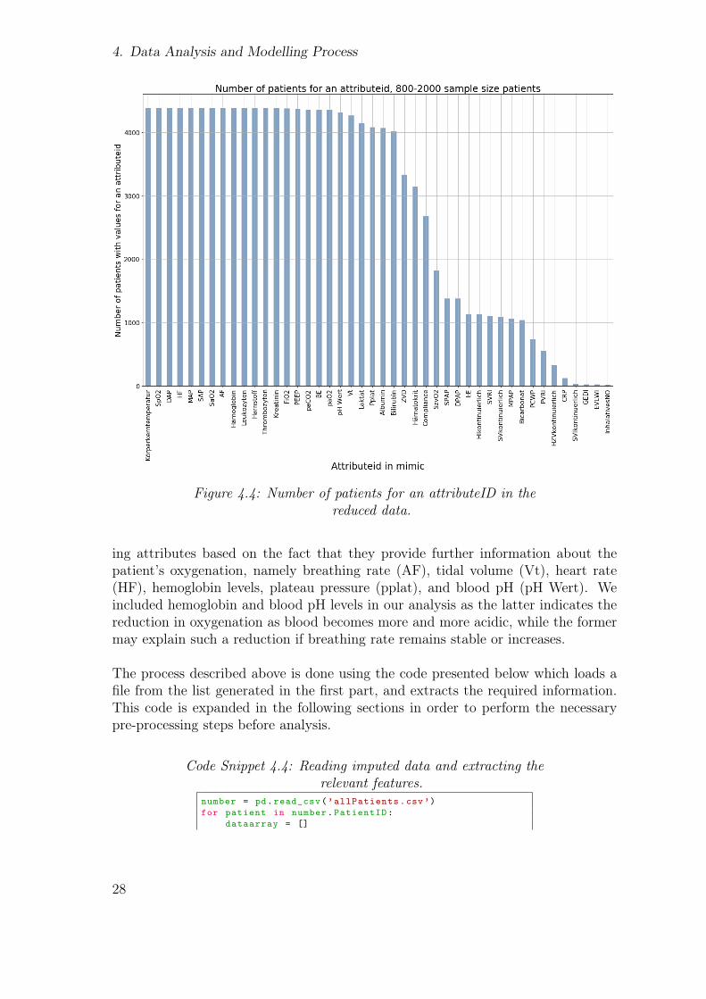
ing attributes based on the fact that they provide further information about thepatient’s oxygenation, namely breathing rate (AF), tidal volume (Vt), heart rate(HF), hemoglobin levels, plateau pressure (pplat), and blood pH (pH Wert). Weincluded hemoglobin and blood pH levels in our analysis as the latter indicates thereduction in oxygenation as blood becomes more and more acidic, while the formermay explain such a reduction if breathing rate remains stable or increases.

The process described above is done using the code presented below which loads afile from the list generated in the first part, and extracts the required information.This code is expanded in the following sections in order to perform the necessarypre-processing steps before analysis.

Code Snippet 4.4: Reading imputed data and extracting therelevant features.

number = pd.read_csv(’allPatients.csv’)for patient in number.PatientID:

dataarray = []

28


ds = feather.read_dataframe("mimic/data {0}. feather↪→ ".format(patient))

data = ds[[’charttime ’,’AF’,’Vt’,’PEEP’,’Pplat’,’↪→ FiO2’,’paO2’,’Hämoglobin ’,’HF’,’pH Wert’]]

4.3.3. Cleaning the Data

When the imputed data was received from our colleagues at Aachen University,they mentioned that missing values within the data were filled out using the meanof their surrounding points. This however did not cover the missing data at thebeginnings and ends of the patient attribute values which we needed to fill. Themethod used also filled in the values with a mean value so as not to affect the signalin any significant way.

After taking care of missing values it was necessary to remove outliers which figurein our plots as spikes in the data and greatly affect the mean and the standarddeviation of the signals. This was done by applying a rolling average function onthe data which resulted in signal smoothing.

Finally, before attempting to cluster in any way, it was necessary to standardise thedata so that the means and standard deviations are within the same ranges. Thiswas done by applying the built-in StandardScaler function of the scikit-learn modulein Python.

The code for the pre-processing that we applied is presented below followed by theplot results for one patient attribute before and after applying the filters.

Code Snippet 4.5: Initial pre-processing steps, revised below.data = data.fillna(data.mean())data = data.fillna (0)X2 = data.iloc [: ,1:]. rolling (10).mean()X2 = X2.fillna(data.mean())X2 = X2.fillna (0)newdata = pd.DataFrame(StandardScaler ().

↪→ fit_transform(X2))newdata.columns = data.drop(columns =[’charttime ’])

↪→ .columns

4.3.4. Constructing the Data

Based on the Berlin Definition, the current standard used to define ARDS onset inmechanically ventilated ICU patients, diagnosis is based on the value of the Horowitz

29


Figure 4.5: Result changes at three steps of pre-processing.

index at 7 days after onset of the injury or of reduced oxygenation as well as otherparameters including PEEP and lung compliance. The Horowitz index is defined asthe ratio of the partial pressure of arterial oxygen (PaO2) to the fraction of inspiredoxygen (FiO2) and it defines the severity of the condition as follows: a measurementis marked as mild ARDS for a value between 300 and 200, moderate for a valuebetween 200 and 100, and severe for a value below 100.

In order to have label generation for our patient set so as to validate the clusteringresults, we implement a model to calculate the Horowitz index of every patient andstore it as a separate column within the patient file. The function to perform thecalculation was obtained from work done by colleagues at Aachen University for thepurposes of their research and implemented at the pre-processing phase of our dataanalysis. The Horowitz value as well as a copy of the PEEP value were preservedwhile the remainder of the parameters were standardised.

After performing the tasks described above, every patient’s data was exported to anindividual file in .csv format so that the calculations need only be done once but thedata can be accessed repeatedly. All of the processes described here are presentedin the code snippet below.

Code Snippet 4.6: Pre-processing the data by applying rollingaverage for smoothing and standardising.

data[’horowitz ’] = horowitz_sample.↪→ calculate_horowitz(data)

X2 = data.iloc [: ,1:]. rolling (10).mean()X2 = X2.fillna(data.mean())X2 = X2.fillna (0)

30

4.4. Modelling

X2[’PEEP2’] = X2.PEEPnewdata = pd.DataFrame(StandardScaler ().

↪→ fit_transform(X2.drop(columns =[’horowitz ’,↪→ ’PEEP2 ’])))

newdata[’horowitz ’] = X2.horowitznewdata[’PEEP2’] = X2.PEEPnewdata.columns = X2.columnsnewdata.to_csv("data -averaged /{0}. csv".format(

↪→ patient), index=False)

4.4. Modelling

4.4.1. Selecting the Modelling Technique

The goal of this project is also to cluster the data in order to draw out of it somerelevant features to our research on ARDS, therefore our modelling technique will beadapted so as to simplify the clustering process. The DBSCAN algorithm that willbe employed to cluster the data is able to find arbitrary-shaped clusters efficientlyas opposed to other available clustering techniques, as discussed in the foundationssection of this report, though it is not well suited to high dimensional data such asthat we have obtained thus far. For that reason we apply methods of reducing thedimensionality of the data, namely Principal Component Analysis (PCA).

In order to apply PCA to the datasets, prior analysis is required to pinpoint thenumber of attributes that best represent the data in question. For this, fitting ofthe PCA function is first performed on the data that is loaded into one file, at whichpoint a graph can be plotted which shows roughly how many attributes are requiredso as to represent the data with adequate precision. After this step, when thenumber of components is selected, PCA is applied and the data is further reducedin such a way that it is better adapted for clustering using DBSCAN.

Additionally, though DBSCAN does not require us to know the number of clustersbeforehand, it does take for input two parameters that need to be determined beforeit can be applied. The epsilon radius is determined by plotting the K-distance graphand selecting the distance at which the curve presents an “elbow.” The minimumnumber of points minpts is selected as either the number of attributes +1 or itsdouble [19]. Finally, through our analysis of the data it became clear that thepotential clusters will not be globular or of any consistent shape, which means thatmore common clustering techniques such as K-means cannot be used. The sectionsthat follow will present the processes by which the above-mentioned values wereselected.

31


4.4.2. Designing the Validation Process

After completing the clustering of our data we aim to validate our results in orderto determine whether the clustering was able to find any relevant patterns in ourdataset. We perform this action so that at the roll-out phase we can be certain thatthe resulting clusters will provide relevant, non-random, information that can beused to diagnose ARDS or highlight the potential that a patient will develop it. Todo this validation step, we will need to highlight which patients did develop ARDSby applying the Berlin Definition of the condition.

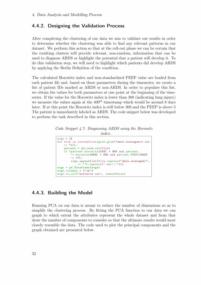
The calculated Horowitz index and non-standardised PEEP value are loaded fromeach patient file and, based on these parameters during the timeseries, we create alist of patient IDs marked as ARDS or non-ARDS. In order to populate this list,we obtain the values for both parameters at one point at the beginning of the time-series. If the value for the Horowitz index is lower than 300 (indicating lung injury)we measure the values again at the 400th timestamp which would be around 8 dayslater. If at this point the Horowitz index is still below 300 and the PEEP is above 5The patient is immediately labeled as ARDS. The code snippet below was developedto perform the task described in this section.

Code Snippet 4.7: Diagnosing ARDS using the Horowitzindex.

avgs = []for file in sorted(list(glob.glob("data -averaged /*.csv

↪→ "))):patient = pd.read_csv(file)if (patient.horowitz [150] < 300 and patient.

↪→ horowitz [400] < 300 and patient.PEEP2 [400]↪→ >7):avgs.append(int(file.replace("data -averaged/",

↪→ ’’).replace(’.csv’,’’)))avgs = pd.DataFrame(avgs)avgs.columns = [’id’]avgs.to_csv(’horowitz.csv’, index=False)

4.4.3. Building the Model

Running PCA on our data is meant to reduce the number of dimensions so as tosimplify the clustering process. By fitting the PCA function to our data we cangraph to which extent the attributes represent the whole dataset and from thatdraw the number of components to consider so that the ultimate results would mostclosely resemble the data. The code used to plot the principal components and thegraph obtained are presented below.

32

4.4. Modelling

Figure 4.6: Component analysis of the data.

Code Snippet 4.8: Determining principal components of thedata based on information content.

# Load all averaged patient data and store them in a↪→ dataframe

allPatients = pd.read_csv(’allPatients.csv’)patients = pd.DataFrame ()for id in allPatients.PatientID:

patients = patients.append(pd.read_csv("data -↪→ averaged /{0}. csv".format(id)))

# Apply PCA to all patients in order to find the↪→ number of

# principal components that most closely represents↪→ the data.

patients = patients.drop(columns =[’horowitz ’,’PEEP2’])pca = PCA().fit(patients)plt.figure(figsize =(20 ,20))plt.grid(True)plt.semilogy(pca.explained_variance_ratio_ ,’--o’)plt.semilogy(pca.explained_variance_ratio_.cumsum (),’

↪→ --o’)plt.savefig(’pca.png’, bbox_inches = "tight")

In the plot we see that we can perform our cutoff at the 5th component since, atthat level, the major part of the data is represented and the information contentis not increasing much; thus we can proceed without risk of affecting our results in

33


a negative way. We apply PCA to the each data file and reduce it to 5 principalcomponents then perform K-nearest neighbour calculations using the "cosine" dis-tance metric for the components over the whole time series and store all the sorteddistance results in one variable. Each row of the resulting dataframe is averagedproducing a list of the average distances within the whole dataset that is then plot-ted and the resulting figure is presented below.

Code Snippet 4.9: Applying PCA and computing theK-distance values.

# Apply PCA based on the number of components that was↪→ decided on.

dist = pd.DataFrame(index=range (0 ,2000))for id in allPatients.PatientID:

pat = pd.read_csv("data -averaged /{0}. csv".format(↪→ id))

comp = pd.DataFrame(PCA(n_components =5).↪→ fit_transform(pat.drop(columns = [’horowitz↪→ ’,’PEEP2’])))

# Save the data of each patient as a separate file↪→ after applying PCA (to reduce read -write cycles↪→ )comp.to_csv("data -pca/comp {0}. csv".format(id),

↪→ index = False)nbrs = NearestNeighbors(n_neighbors =5,algorithm=’

↪→ brute ’,metric=’cosine ’).fit(comp.values[↪→ range(0,len(comp)) ,:])

distance ,indices = nbrs.kneighbors(comp)for i in range(0,len(distance)):

distance[i] = np.average(distance[i,:])distance = pd.DataFrame(sorted(distance [:,0]))distance = distance.iloc [::-1]distance = distance.reset_index ()distance = distance.drop(columns=’index’)dist = pd.concat ([dist ,distance],axis = 1)

dist.columns = allPatients.PatientID# Compute the average of the k-distances and plot the

↪→ k-distance graphavg = []for i in range (0 ,2000):

avg.append(np.average(dist.values[i,:]))plt.figure(figsize =(15 ,15))plt.grid(True)plt.plot(avg)plt.savefig(’distance.png’, bbox_inches = "tight")

Selecting the epsilon value for DBSCAN is not a straightforward approach butrather requires a bit tuning. From the distance graph in Figure 4.7 we select epsilonbetween 0,01 and 0,02. As for minpts we will perform clustering based on both rec-ommended values (dim+1 and dim*2) [19] and study other potential values usingthe gridsearch method. Additionally, the clustering is done at one point for all thepatient files, which is a point 4 days after initial signs of lung injury. The code belowdescribes how DBSCAN is applied to the data.

34

4.4. Modelling

Figure 4.7: K-distance graph of the data.

Code Snippet 4.10: Applying the DBSCAN algorithm andsaving the results to an output file.

# Select a specific timepoint for every patient and↪→ store in a dataframe

start = time.time()extract = []for file in list(glob.glob("data -pca/*.csv")):

comp = pd.read_csv(file)extract.append(comp.values [300 ,:])

extract = pd.DataFrame(extract)# Apply DBSCAN clustering on the selected timepoint

↪→ for each# patient with eps selected based on the k-distance

↪→ graph.clust = cluster.DBSCAN(eps =0.015 , min_samples =10,

↪→ metric=’cosine ’)q = clust.fit_predict(extract)allPatients[’clusters ’] = qallPatients.to_csv(’results.csv’)end = time.time()print(end -start) # Displays the total time to complete

↪→ this task in seconds

Finally, given that there is a large amount of data that needs to be processed andan equally large amount that is produced in our attempt to cluster patients for

35


ARDS diagnosis, we proposed to run the code using parallel computing technologyin order to gauge the potential speed-up that may be achieved when running suchdata- and compute-intensive applications on a supercomputer as opposed to runningthem on a local machine. Pre-processing the data and creating individual patientfiles, and loading the data to calculate distances are the two steps that require themost computing time and power and are therefore the parts of the data that can beparallelised so as to speed up the analysis process.

4.4.4. Assessing the Model

The final part to consider in the modelling phase of this project is the assessment ofour parameter selection in terms of the clustering method and the number of coresin running the compute-intensive parts of the code.

When it comes to applying DBSCAN to our data, simply selecting values for epsilonand minpts may not mean that the best values were selected; therefore, we imple-ment a grid search method to provide a list of the most effective combinations ofthe two parameters. This method, the code for which is provided below, was imple-mented both in a serial and a parallel environment and the speed-up was recorded.The results are also presented in a Figure 5.2 and will be further investigated in theevaluation chapter that will follow.

Code Snippet 4.11: Applying gridsearch in serial.eps = list(range (5,26))eps [:] = [x / 1000 for x in eps]minpts = list(range (6 ,27))grid = pd.DataFrame(index=minpts , columns=eps)start = time.time()extract = []for file in list(glob.glob(’/data -pca /*.csv’)):


extract = pd.DataFrame(extract)for i in minpts:

for j in eps:# Apply DBSCAN clustering on the selected timepoint

↪→ for each# patient with eps selected based on the k-distance

↪→ graph.clust = cluster.DBSCAN(eps=j, min_samples=i,

↪→ metric=’cosine ’)q = clust.fit_predict(extract)grid.values[i-6,int(j*1000 -5)] = len(np.unique

↪→ (q))-1end = time.time()print(end -start)

Running any snippet of code in parallel requires a different approach to solving the

36

4.4. Modelling

problem and for that reason it is not often straightforward to select the number ofcores to call on to run our code. In the case of the data preparation step, we judgedthat running the program on one node should be sufficient to achieve a significantspeed-up, given that a node has 48 cores. On the other hand using 48 cores torun the gridsearch code below would be wasteful and counterproductive as in eitherdimension, the selected range is 21 steps, so we can break the first for loop andassign 21 cores with the task of running the remainder of the loop to complete theclustering implementation.

37

5. Evaluation

5.1. Experimental Setup

In this chapter we break down our results in order to draw our conclusions as to theeffectiveness of the approaches that were implemented in our attempt to answer theresearch questions posed at the beginning of this report. By continuing with theCRISP-DM process with respect to model evaluation, we need a proper experimentalsetup over which to perform our evaluation. This section of the chapter analyses thecomputing and data infrastructures, as well as tools and methods that were used inthe process and highlights the key aspects of the methods by which the results willbe judged.

We opted to perform our benchmarking steps for speed-up related to large scaledata-processing applications using a laptop computer and the JURON and DEEP-ER SDV HPC clusters. While not loosing sight of general usability elements withJupyter, the idea is to show the speed-up that can be achieved with the properarchitecture. Similarly, we needed to program certain elements of the applicationfor running in parallel and making use of the available threads, which allowed us togauge the speed-up of the data processing between parallel and serial programmingon the same system. Tables 5.1 and 5.2 present the specifications of the two HPCclusters employed in the parallelisation approach.

Table 5.1: Technical specifications of each of the servers in theJURON cluster[2].

Processor 2 IBMPOWER8 processors (up to 4.023GHz, 2x 10cores, 8 threads/core)

Memory 256GB DDR4 attached to CPUGPU 4 NVIDIA Tesla P100 ("Pascal")Memory 4x16 GByte HBM memory attached to GPUNon-Volatile Memory ∼ 1TB GST Ultrastar SN100 Series NVMe SSDOperating System CentOS 7.3, Linux kernel 3.10.0-514.21.1.el7

When it comes to software, the Jupyter Notebook was a major tool in writing,testing, running, and evaluating the code that would extract the data and perform

39

5. Evaluation

Table 5.2: Technical specifications of the DEEP-ER SDVPrototype[3].

Cluster 16 dual-socket Intel R© Xeon R© E5-2680v3 nodesCluster Memory 128GB DRAM, 400GB NVMBooster 8 Adams Pass Intel Xeon Phi 7210 CPUBooster Memory/Node 16GB on-package memory, 96GB DRAM, 200GB

NVMStorage 2 storage servers (spinning disks, 57TB)

the necessary pre-processing steps before clustering. For that reason, being able touse it in order to perform the same tasks that would be done locally, but on a largescale HPC cluster was extremely convenient and was instrumental in completing theresearch that we set out to perform. It is worth noting that, until the implementationof this tool into the parallel computing environment, all tasks to be performed ona supercomputer had to involve job scripts and required the user to run all of theircode every time in one go. The benefit of using the Jupyter Notebook on HPC inthis case, regardless of it still being a work in progress and only a recent endeavour,is the fact that it offers the added convenience of providing a graphical interface tovisualise the code and the output at the same time and of running only part of thecode as desired, thus allowing us to break down the tasks into parts and measurespeed up over all of them. The Jupyter environment can be also easily extendedfor future studies in ARDS and is thus massively flexible for further research bymedical doctors. Additionally, the research in this thesis contributed to overcomingissues with technical job scripts, ssh logins and keys, and other technical elementsby focusing on a seamless approach that can also be used by non-technical-savvymedical experts.

5.2. Evaluating Relevance of Data and CodeProvisioning for ARDS

Although our main goal in the data preparation and pre-processing phases was toproduce samples with high relevance to the condition in question, we also aimedto reduce the datasets in size as much as possible. On the one hand this processwould reduce noise from either irrelevant or inconsistently recorded attributes, whileon the other hand it allowed a reduction in the density of the data manipulationjob. Ultimately the selected attributes were judged as the most relevant to ARDSdiagnosis based on the likelihood that a patient will have values recorded for theseattributes in their record, but also based on our prior understanding of the conditionand of physiology. Figure 5.1 below presents the different stages of the data, as well

40

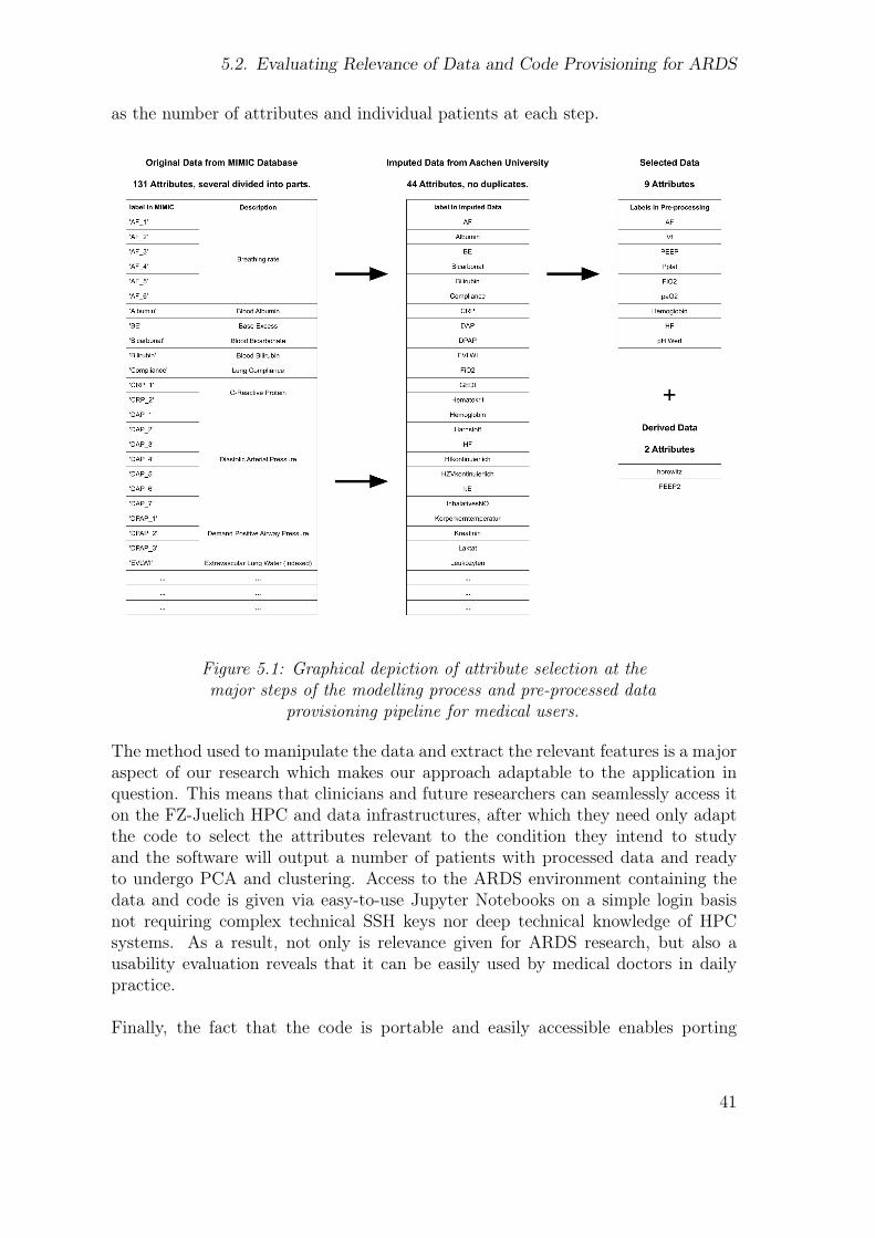
5.2. Evaluating Relevance of Data and Code Provisioning for ARDS

as the number of attributes and individual patients at each step.

Figure 5.1: Graphical depiction of attribute selection at themajor steps of the modelling process and pre-processed data

provisioning pipeline for medical users.

The method used to manipulate the data and extract the relevant features is a majoraspect of our research which makes our approach adaptable to the application inquestion. This means that clinicians and future researchers can seamlessly access iton the FZ-Juelich HPC and data infrastructures, after which they need only adaptthe code to select the attributes relevant to the condition they intend to studyand the software will output a number of patients with processed data and readyto undergo PCA and clustering. Access to the ARDS environment containing thedata and code is given via easy-to-use Jupyter Notebooks on a simple login basisnot requiring complex technical SSH keys nor deep technical knowledge of HPCsystems. As a result, not only is relevance given for ARDS research, but also ausability evaluation reveals that it can be easily used by medical doctors in dailypractice.

Finally, the fact that the code is portable and easily accessible enables porting

41

5. Evaluation

the Jupyter script to cloud infrastructures like the European Open Science Clouds(EOSC-Nordic) [28]

5.3. Pre-processing and Clustering ResultEvaluation

One of the research questions of this thesis was to apply HPC to prepare for largerupcoming versions of the MIMIC database in general and to enable a speed-up andinteractive clustering for users. In Section 1 of Chapter 4, our approach to modellingrequired comparing results obtained from a local machine with those obtained froma parallel application of the adapted code. For that purpose we attempted to runthe code locally, though it became immediately obvious that the processing powerand memory were not enough to complete the tasks required. For that reason, andeven though our main focus is on the potential speed-up that parallelising may offer,we will also make note of the effect that running such data- and compute-intensiveapplications on a local machine can have.

In the data preparation and pre-processing phases, the most time and energy con-suming part of the code involves reading from the imputed data files, extracting therelevant information and then storing in separate files in csv format. The speed-upfor this process is presented in Table 5.3 below.

Table 5.3: Time required to complete the pre-processingsection of the code on each type of architecture.

Local JURON Serial Parallel (48 cores)1099,99 seconds 2370,72 seconds 68,32 seconds

It is worth mentioning that though the process took longer as a serial application onthe JURON cluster than on the laptop, the latter was clearly beginning to exhibitperformance issues including overheating and lag.

After applying PCA to the dataset and reducing it to five principal components,clustering was attempted and we immediately realised that the output would begreatly dependent on the selected parameters of epsilon and minpts as the resultswould vary greatly. Additionally our approach required comparison of the clusteringresults to the diagnosis obtained by using the Horowitz index as per the Berlindefinition of ARDS. This process proved difficult and thus we decided to rely on thegridsearch method to find the best combination of the parameters. The steps thatfollowed are discussed below where we discuss the parallel and serial implementationsof gridsearch as well as the ultimate results.

42

5.4. Gridsearch Result Evaluation

5.4. Gridsearch Result Evaluation

Performing the gridsearch to find the most effective range of values for minpts andepsilon on a local machine required a total of 215,15 seconds (3,58 minutes) while inparallel it completed in 40,17 seconds. Another iteration of the code was preparedthat allowed for scaling up the number of processors and increasing the range ofminpts and epsilon which ran the code in 64,42 seconds. Finally, one early versionof this code was inefficient and required a total of 3 hours to complete in serial onJURON while in parallel completed in 1093,04 seconds (18 minutes). The resultsof the output of the gridsearch code is presented below in Figure 5.2 with the mostviable parameter highlighted in green, and acceptable values in yellow.

Figure 5.2: Different possible combinations of minpts andepsilon and the number of clusters produced

5.5. Review of Applied Processes

Using the gridsearch method described in Section 4, we select a few values for theDBSCAN parameters to attempt clustering the patients. In order to validate theeffectiveness of clustering we implemented the Berlin definition of diagnosing ARDSand were able to highlight some patients as fulfilling the criteria for the condition.We implemented the code below in order to cross match patient IDs that appear in

43

5. Evaluation

both the main patient list and the Horowitz list. Of course, this evaluation is onlyfor showing technical feasibility of the selected approach while more research frommedical experts is needed to derive medically relevant results from clustering suchas detecting early stage ARDS for example.

Code Snippet 5.1: Writing diagnosis results in the output file.allPatients = pd.read_csv(’allPatients.csv’)allPatients[’ards’] = 0allPatients = allPatients.set_index(’PatientID ’)ards = pd.read_csv(’horowitz.csv’)for i in ards.id:

allPatients.loc[i].ards = 1allPatients.to_csv(’allPatients.csv’)

Similarly, when clustering is performed based on the chosen parameter values, theresults are also written into the main patients list. Thus we were able to comparethe results of clustering for the four parameter values highlighted in Figure 5.2 withthose of the diagnosis process. Figure 5.3 presented below highlights the differencesthat small changes in the parameters would cause in how the data is understood. Weunderline the fact that in this case the clustering results for only 2 of the 5 principalcomponents are presented. On the other hand, Figure 5.4 shows the diagnosis resultsbased on the Horowitz index and highlights the fact that further work needs to bedone from medical experts that take advantage of the results of this master thesisin order to improve the clustering results.

We note that, in general, an early detection of the ARDS is a hot topic in researchconcerning this condition, especially given the challenging situation that the timeseries data recordings of ICU patients are usually only often short or inconsistent.This in turn makes it difficult to detect patterns and highlights the potential benefitthat unsupervised methods may to have in ARDS research today.

44

5.5. Review of Applied Processes

Figure 5.3: Four different clustering results with theirrespective parameters.

45

5. Evaluation

Figure 5.4: ARDS patients as diagnosed using the Horowitzindex.

46

6. Conclusion

In this thesis we presented our work of preparing and exploring data by performingthe analysis of large scale data from healthcare with a particular focus on ARDSpatients, and the attempt of using state-of-the-art technology in HPC, unsupervisedlearning, and parallel programming in order to highlight features within the analyseddata. In our approach, we developed a Python code that reads patient data fromclinical database entries, selects a set of the most well-represented parameters relatedto the condition in question, in this case ARDS, and performs the necessary pre-processing steps to prepare this data for clustering.

Additionally, our aim was to highlight the potential benefits of using HPC tech-nology and our knowledge in parallel programming techniques to accelerate thework and reduce the workload which ultimate proved successful given the speed-upthat was observed in our applications. This was done using an HPC- and parallelcomputing-ready version of the Jupyter Notebook which recently became availableon the JURON cluster of FZ-Juelich, and is the product of years of research towardsmaking parallel computing more accessible despite of the fact that it is usually ratherbatch-driven instead of interactive. Given the fact that our approach takes advan-tage of the availability of Jupyter in a parallel environment, we believe our workopens up the path for clinicians to begin using this technology in their work, a stepwhich would have been improbable with traditional HPC approaches.

Finally, we applied DBSCAN clustering in order to highlight structures in the datathat could be used in the diagnosis of ARDS. Afterwards, we implemented a gridsearch algorithm that was able to output the most effective combinations of param-eters for clustering. In parallel, and using the literature on ARDS diagnosis, wecoded a program that listed the IDs of all patients that fit the criteria of the Berlindefinition and attempted to use its result to evaluate our clustering technique. Toconclude, the thesis results pave the way with a sound technical solution of makingARDS research faster yet flexible and usable for clinicians today.

As a product developed under the scope of several institutions, the code describedin this project will be available to all participants in the SMITH project throughaccess to the FZ-Juelich HPC and data infrastructure. One of the next steps ofthis thesis is to explore the possibility to make the code and data available in theResearch Data Alliance (RDA) Interest Group (IG) on Big Data that is co-chaired

47

6. Conclusion

by FZ-Juelich. This is useful to expose the thesis findings to a broader internationalaudience and goes far beyond the SMITH consortium.

The code is going to be edited, adapted, and used on a somewhat regular basis aspart of the ASIC use case of the SMITH project as well as other potential uses whereother researchers might see fit, therefore it will receive maintenance in a consistentmanner. In light of the close cooperation of the University of Iceland and FZ-Juelichin several medical projects, the idea is to work together with Lanspítalinn in thecontext of ARDS in general and with the developed thesis approaches in particular.

Concerning future work in this field, our future research will most certainly revolvearound discovering patterns of how the clustered patients are similar, what theiridentifying features are, and how this understanding can help improve future clus-tering results. Additionally, it would be interesting to focus further on the sizesof the created clusters, instead of only looking at the number, and finding ways tomaximise that size. Similarly, given the easy access to HPC technology, it would befeasible to cluster at several points of the timeseries data in order to visualise howthe patients are evolving towards or away from being diagnosed as ARDS.

On the other hand, we might also consider developing methods to parallelise differentparts of the pre-processing phase, PCA implementation, and K-distance calculation.The code will constantly be revised so that it can be easily implemented whereneeded and adapted to the research questions posed in this thesis as the outcomesof this research with respect to pre-processing are also suitable for research in otherconditions in the ICU. Furthermore, we see potential in adapting our processes formore advanced clinical applications and use cases with large scale datasets wheretraditional approaches have failed.

48

Bibliography

[1] A. E. Johnson, T. J. Pollard, L. Shen, L.-w. H. Lehman, M. Feng, M. Ghassemi,B. Moody, P. Szolovits, L. Anthony Celi, and R. G. Mark, “MIMIC-III, afreely accessible critical care database,” Scientific Data, vol. 3, no. 160035,May 2016. [Online]. Available: https://doi.org/10.1038/sdata.2016.35

[2] A. Eekhoff, B. Tweddell, and D. Pleiter, “BeeGFS Benchmarks on JURON,” oct2017. [Online]. Available: https://www.beegfs.io/docs/whitepapers/JURON_OpenPOWER_NVMe_by_ThinkParQ_FZ-Juelich.pdf

[3] “DEEPprojects prototypes,” 2017. [Online]. Available: https://www.deep-projects.eu/hardware/prototypes.html

[4] A. Winter, S. Stäubert, D. Ammon, S. Aiche, O. Beyan, V. Bischoff,P. Daumke, S. Decker, G. Funkat, J. E. Gewehr, A. de Greiff, S. Haferkamp,U. Hahn, A. Henkel, T. Kirsten, T. Klöss, J. Lippert, M. Löbe, V. Lowitsch,O. Maassen, J. Maschmann, S. Meister, R. Mikolajczyk, M. Nüchter,M. W. Pletz, E. Rahm, M. Riedel, K. Saleh, A. Schuppert, S. Smers,A. Stollenwerk, S. Uhlig, T. Wendt, S. Zenker, W. Fleig, G. Marx,A. Scherag, and M. Löffler, “Smart medical information technology forhealthcare (SMITH),” Methods Inf Med, vol. 27, no. 1, 2018. [Online].Available: https://doi.org/10.3414/ME18-02-0004

[5] B. K. Beaulieu-Jones, P. Orzechowski, and J. H. Moore, “Mappingpatient trajectories using longitudinal extraction and deep learning in theMIMIC-III critical care database,” bioRxiv, aug 2017. [Online]. Available:https://doi.org/10.1101/177428

[6] “Report on the workshop on "High Performance Computing in Health Re-search",” 2014. [Online]. Available: https://ec.europa.eu/digital-single-market/en/news/workshop-high-performance-computing-hpc-health-research

[7] P. F. Ghalati, S. S. Samal, J. S. Bhat, R. Deisz, G. Marx, and A. Schuppert,“Critical transitions in intensive care units: A sepsis case study,” arXive-prints, 02 2019. [Online]. Available: https://arxiv.org/pdf/1902.05764.pdf

[8] M. Komorowski, L. A. Celi, O. Badawi, A. Gordon, and A. Faisal, “Theartificial intelligence clinician learns optimal treatment strategies for sepsis

49

https://doi.org/10.1038/sdata.2016.35

https://www.beegfs.io/docs/whitepapers/JURON_OpenPOWER_NVMe_by_ThinkParQ_FZ-Juelich.pdf

https://www.beegfs.io/docs/whitepapers/JURON_OpenPOWER_NVMe_by_ThinkParQ_FZ-Juelich.pdf

https://www.deep-projects.eu/hardware/prototypes.html

https://www.deep-projects.eu/hardware/prototypes.html

https://doi.org/10.3414/ME18-02-0004

https://doi.org/10.1101/177428

https://ec.europa.eu/digital-single-market/en/news/workshop-high-performance-computing-hpc-health-research

https://ec.europa.eu/digital-single-market/en/news/workshop-high-performance-computing-hpc-health-research

https://arxiv.org/pdf/1902.05764.pdf

BIBLIOGRAPHY

in intensive care,” Nature Medicine, vol. 24, 10 2018. [Online]. Available:https://doi.org/10.1038/s41591-018-0213-5

[9] V. Huddar, K. Desiraju, V. Rajan, S. Bhattacharya, S. Roy, andC. Reddy, “Predicting complications in critical care using heterogeneousclinical data,” IEEE Access, vol. 4, pp. 1–1, 01 2016. [Online]. Available:https://doi.org/10.1109/ACCESS.2016.2618775

[10] M. Afshar, C. Joyce, A. Oakey, P. Formanek, P. Yang, M. Churpek, R. Cooper,S. Zelisko, R. Price, and D. Dligach, “A computable phenotype for acute respi-ratory distress syndrome using natural language processing and machine learn-ing,” AMIA ... Annual Symposium proceedings. AMIA Symposium, vol. 2018,pp. 157–165, 12 2018.

[11] A. Das, M. Haque, M. Chikhani, W. Wang, J. G. Hardman, andD. G. Bates, “Creating virtual ARDS patients,” in 2016 38th AnnualInternational Conference of the IEEE Engineering in Medicine andBiology Society (EMBC), Aug 2016, pp. 2729–2732. [Online]. Available:https://doi.org/10.1109/EMBC.2016.7591294

[12] D. G. Ashbaugh, D. B. Bigelow, T. L. Petty, and B. E. Levine, “Acuterespiratory distress in adults,” The Lancet, vol. 290, no. 7511, pp. 319 –323, 1967, originally published as Volume 2, Issue 7511. [Online]. Available:http://www.sciencedirect.com/science/article/pii/S0140673667901687

[13] P. Chapman, “The CRISP-DM user guide,” 1999. [Online]. Available:https://s2.smu.edu/~mhd/8331f03/crisp.pdf

[14] The ARDS Definition Task Force, “Acute Respiratory Distress Syndrome: TheBerlin Definition of ARDS,” JAMA, vol. 307, no. 23, pp. 2526–2533, Jun 2012.[Online]. Available: https://doi.org/10.1001/jama.2012.5669

[15] J. Villar, J. Blanco, J. M. Añón, A. Santos-Bouza, L. Blanch, A. Ambrós,F. Gandía, D. Carriedo, F. Mosteiro, S. Basaldúa, R. L. Fernández, R. M.Kacmarek, and the ALIEN Network, “The ALIEN study: incidence andoutcome of acute respiratory distress syndrome in the era of lung protectiveventilation,” Intensive Care Medicine, vol. 37, no. 12, pp. 1932–1941, Dec2011. [Online]. Available: https://doi.org/10.1007/s00134-011-2380-4

[16] L. D. Bos, L. R. Schouten, L. A. van Vught, M. A. Wiewel, D. S. Y. Ong,O. Cremer, A. Artigas, I. Martin-Loeches, A. J. Hoogendijk, T. van der Poll,J. Horn, N. Juffermans, C. S. Calfee, and M. J. Schultz, “Identification andvalidation of distinct biological phenotypes in patients with acute respiratorydistress syndrome by cluster analysis,” Thorax, vol. 72, no. 10, pp. 876–883,2017. [Online]. Available: https://thorax.bmj.com/content/72/10/876

50

https://doi.org/10.1038/s41591-018-0213-5

https://doi.org/10.1109/ACCESS.2016.2618775

https://doi.org/10.1109/EMBC.2016.7591294

http://www.sciencedirect.com/science/article/pii/S0140673667901687

https://s2.smu.edu/~mhd/8331f03/crisp.pdf

https://doi.org/10.1001/jama.2012.5669

https://doi.org/10.1007/s00134-011-2380-4

https://thorax.bmj.com/content/72/10/876

BIBLIOGRAPHY

[17] C. S. Calfee, K. Delucchi, P. E. Parsons, B. T. Thompson, L. B. Ware, M. A.Matthay, and the NHLBI ARDS Network, “Subphenotypes in acute respiratorydistress syndrome: latent class analysis of data from two randomised controlledtrials,” Respiratory Medicine, vol. 2, no. 8, May 2015. [Online]. Available:https://doi.org/10.1016/S2213-2600(14)70097-9

[18] S. Shalev-Shwartz, S. Ben-David, and Cambridge Univer-sity Press, Understanding Machine Learning: From The-ory to Algorithms. Cambridge University Press, 2015. [Online].Available: https://www.cs.huji.ac.il/~shais/UnderstandingMachineLearning/understanding-machine-learning-theory-algorithms.pdf

[19] M. Ester, H.-P. Kriegel, J. Sander, and X. Xu, “A density-based algorithmfor discovering clusters in large spatial databases with noise,” in Proceedingsof the Second International Conference on Knowledge Discovery and DataMining, ser. KDD’96. AAAI Press, 1996, pp. 226–231. [Online]. Available:http://dl.acm.org/citation.cfm?id=3001460.3001507

[20] P.-N. Tan, M. Steinbach, A. Karpatne, and V. Kumar, Introduction to DataMining. Pearson, 2005.

[21] G. Hager and G. Wellein, Introduction to High Performance Computing forScientists and Engineers. Chapman & Hall/CRC Computational Science, 2010.

[22] M. Götz, C. Bodenstein, and M. Riedel, “HPDBSCAN: Highly parallelDBSCAN,” in Proceedings of the Workshop on Machine Learning inHigh-Performance Computing Environments, ser. MLHPC ’15. NewYork, NY, USA: ACM, 2015, pp. 2:1–2:10. [Online]. Available: https://doi.org/10.1145/2834892.2834894

[23] “Project jupyter.” [Online]. Available: https://jupyter.org/

[24] “Intellispace critical care and anesthesia.” [Online]. Avail-able: https://www.philips.co.uk/healthcare/product/HCNOCTN332/intellispace-critical-care-and-anesthesia

[25] M. Götz, M. Kononets, C. Bodenstein, M. Riedel, M. Book, and O. P. Palsson,“Automatic water mixing event identification in the koljö fjord observatorydata,” International Journal of Data Science and Analytics, vol. 7, no. 1, pp. 67–79, Feb 2019. [Online]. Available: https://doi.org/10.1007/s41060-018-0132-z

[26] “Python data analysis library.” [Online]. Available: https://pandas.pydata.org/

[27] “feather-format.” [Online]. Available: https://pypi.org/project/feather-format/

[28] “European open science cloud.” [Online]. Available: https://www.eosc-portal.eu/

51

https://doi.org/10.1016/S2213-2600(14)70097-9

https://www.cs.huji.ac.il/~shais/UnderstandingMachineLearning/understanding-machine-learning-theory-algorithms.pdf

https://www.cs.huji.ac.il/~shais/UnderstandingMachineLearning/understanding-machine-learning-theory-algorithms.pdf

http://dl.acm.org/citation.cfm?id=3001460.3001507

https://doi.org/10.1145/2834892.2834894

https://doi.org/10.1145/2834892.2834894

https://jupyter.org/

https://www.philips.co.uk/healthcare/product/HCNOCTN332/intellispace-critical-care-and-anesthesia

https://www.philips.co.uk/healthcare/product/HCNOCTN332/intellispace-critical-care-and-anesthesia

https://doi.org/10.1007/s41060-018-0132-z

https://pandas.pydata.org/

https://pypi.org/project/feather-format/

https://www.eosc-portal.eu/

https://www.eosc-portal.eu/

A. Appendix

Code Snippet A.1: The code that was developed for this thesis.This code is only meant for serial implementation.

import numpy as npimport pandas as pdimport matplotlib.pyplot as pltimport mathimport globimport timeimport horowitz_samplefrom sklearn.neighbors import NearestNeighborsfrom sklearn.decomposition import PCAfrom sklearn.preprocessing import StandardScalerfrom sklearn import clusterfrom scipy import signalfrom scipy import stats

# Query the database and print Figure \ref{fig:mimic}import helperscnx = helpers.getCnx("mimic_oracle")

data = pd.read_excel(’mimic_factor.xlsx’)attids = data.itemidlabels = data.label

params_intersection = pd.DataFrame ()for i,attr in enumerate(attids):

query = """(select distinct(subject_id) from labevents where↪→ itemid ={0}) union (select distinct(subject_id) from↪→ chartevents where itemid ={0}) """.format(attr)

query = query.replace(’[’, ’(’).replace(’]’, ’)’)data = pd.read_sql(query , cnx)params_intersection = pd.concat ([ params_intersection ,data],

↪→ ignore_index=True , axis =1)print(i)

params_intersection.columns = attidsparams_intersection.columns = labels# for each attribute ID list the number of admissionswidth = 18height = 14plt.figure ()params_intersection.count().sort_values(ascending = False).plot.

↪→ bar(figsize =(width ,height), color =(0.2 ,0.4 ,0.6 ,0.6))ax = plt.gca()ax.set_ylabel("Number of admissions with values for an attributeid

↪→ ", size = 20)ax.set_title(’Number of admissions for an attributeid , mimic ’,

↪→ size = 24)ax.set_xlabel(’Attributeid in mimic’, size = 24)ax.grid(True)ax.tick_params(axis=’both’, which=’major’, labelsize =16)plt.tight_layout ()

53

A. Appendix

plt.show()

# Query imputed data and print Figure \ref{fig:imputed}for file in list(glob.glob("mimic /*. feather")):

ds = feather.read_dataframe(file)abc = ds.isna().all()abc ^= Trueabc = abc.rename(file.replace(’mimic/data’,’’).replace(’.

↪→ feather ’,’’))out = out.append(abc.drop(’charttime ’))

out.sum(axis =0).sort_values(ascending = False).plot.bar(figsize =(↪→ width ,height), color =(0.2 ,0.4 ,0.6 ,0.6))

# Prepare a list of patients fitting within the set window of↪→ samples

samples = 200times = []for file in sorted(list(glob.glob("mimic /*. feather"))):

patient = feather.read_dataframe(file)if (4* samples < len(patient.charttime) < 10* samples):

times.append ([id])times = pd.DataFrame(times)times.columns = [’PatientID ’]times.to_csv(’allPatients.csv’, index=False)

# Perform Pre -processingnumber = pd.read_csv(’allPatients.csv’)for patient in number.PatientID:

dataarray = []ds = feather.read_dataframe("mimic/data {0}. feather".format(

↪→ patient))data = ds[[’charttime ’,’AF’,’Vt’,’PEEP’,’Pplat’,’FiO2’,’paO2’,

↪→ ’Hämoglobin ’,’HF’,’pH Wert’]]data[’horowitz ’] = horowitz_sample.calculate_horowitz(data)X2 = data.iloc [: ,1:]. rolling (10).mean()X2 = X2.fillna(data.mean())X2 = X2.fillna (0)X2[’PEEP2’] = X2.PEEPnewdata = pd.DataFrame(StandardScaler ().fit_transform(X2.drop(

↪→ columns =[’horowitz ’, ’PEEP2 ’])))newdata[’horowitz ’] = X2.horowitznewdata[’PEEP2’] = X2.PEEPnewdata.columns = X2.columnsnewdata.to_csv("data -averaged /{0}. csv".format(patient), index=

↪→ False)

# Diagnose ARDS based on Horowitz indexavgs = []for file in sorted(list(glob.glob("data -averaged /*.csv"))):

patient = pd.read_csv(file)if (patient.horowitz [150] < 300 and patient.horowitz [400] <

↪→ 300 and patient.PEEP2 [400] >7):avgs.append(int(file.replace("data -averaged/",’’).replace(

↪→ ’.csv’,’’)))avgs = pd.DataFrame(avgs)avgs.columns = [’id’]avgs.to_csv(’horowitz.csv’, index=False)

# Load all averaged patient data and store them in a dataframeallPatients = pd.read_csv(’allPatients.csv’)patients = pd.DataFrame ()for id in allPatients.PatientID:

patients = patients.append(pd.read_csv("data -averaged /{0}. csv"↪→ .format(id)))

# Apply PCA to all patients in order to find the number of# principal components that most closely represents the data.

54

patients = patients.drop(columns =[’horowitz ’,’PEEP2’])pca = PCA().fit(patients)plt.figure(figsize =(20 ,20))plt.grid(True)plt.semilogy(pca.explained_variance_ratio_ ,’--o’)plt.semilogy(pca.explained_variance_ratio_.cumsum (),’--o’)plt.savefig(’pca.png’, bbox_inches = "tight")

# Apply PCA based on the number of components that was decided on↪→ from Figure \ref{fig:pca}.

dist = pd.DataFrame(index=range (0 ,2000))for id in allPatients.PatientID:

pat = pd.read_csv("data -averaged /{0}. csv".format(id))comp = pd.DataFrame(PCA(n_components =5).fit_transform(pat.drop

↪→ (columns = [’horowitz ’,’PEEP2’])))# Save the data of each patient as a separate file after applying

↪→ PCA (to reduce read -write cycles)comp.to_csv("data -pca/comp {0}. csv".format(id), index = False)nbrs = NearestNeighbors(n_neighbors =5,algorithm=’brute ’,metric

↪→ =’cosine ’).fit(comp.values[range(0,len(comp)) ,:])distance ,indices = nbrs.kneighbors(comp)for i in range(0,len(distance)):

distance[i] = np.average(distance[i,:])distance = pd.DataFrame(sorted(distance [:,0]))distance = distance.iloc [::-1]distance = distance.reset_index ()distance = distance.drop(columns=’index’)dist = pd.concat ([dist ,distance],axis = 1)

dist.columns = allPatients.PatientID# Compute the average of the k-distances and plot the k-distance

↪→ graph from Figure \ref{fig:distance}avg = []for i in range (0 ,2000):

avg.append(np.average(dist.values[i,:]))plt.figure(figsize =(15 ,15))plt.grid(True)plt.plot(avg)plt.savefig(’distance.png’, bbox_inches = "tight")

# Select a specific timepoint for every patient and store in a↪→ dataframe

start = time.time()extract = []for file in list(glob.glob("data -pca/*.csv")):


extract = pd.DataFrame(extract)# Apply DBSCAN clustering on the selected timepoint for each# patient with eps selected based on the k-distance graph.clust = cluster.DBSCAN(eps =0.015 , min_samples =10, metric=’cosine ’)q = clust.fit_predict(extract)allPatients[’clusters ’] = qallPatients.to_csv(’results.csv’)end = time.time()print(end -start) # Displays the total time to complete this task

↪→ in seconds

# Save ARDS Diagnosis results into main patient fileallPatients = pd.read_csv(’allPatients.csv’)allPatients[’ards’] = 0allPatients = allPatients.set_index(’PatientID ’)ards = pd.read_csv(’horowitz.csv’)for i in ards.id:

allPatients.loc[i].ards = 1allPatients.to_csv(’allPatients.csv’)

55

A. Appendix

# Perform Gridsearcheps = list(range (5,26))eps [:] = [x / 1000 for x in eps]minpts = list(range (6 ,27))grid = pd.DataFrame(index=minpts , columns=eps)start = time.time()extract = []for file in list(glob.glob(’/data -pca /*.csv’)):


extract = pd.DataFrame(extract)for i in minpts:

for j in eps:# Apply DBSCAN clustering on the selected timepoint for each# patient with eps selected based on the k-distance graph.

clust = cluster.DBSCAN(eps=j, min_samples=i, metric=’↪→ cosine ’)

q = clust.fit_predict(extract)grid.values[i-6,int(j*1000 -5)] = len(np.unique(q)) -1

end = time.time()print(end -start)

56

modelling and evaluation of serial and parallel density

Documents