modelling and simulation of research concept...
TRANSCRIPT

Modelling and simulation of Research Concept Vehicle using MBD-FEM
approach
Tarun Mallikarjuna Rao
Master of Science Thesis MMK 2015:105 MKN 148
KTH Industrial Engineering and Management
Machine Design SE-100 44 STOCKHOLM

Modelling and simulation of Research Concept Vehicle using MBD-FEM approach
Tarun Mallikarjuna Rao
Master of Science Thesis MMK 2015:105 MKN 148
KTH Industrial Engineering and Management
Machine Design
SE-100 44 STOCKHOLM

i
Examensarbete MMK 2015:105 MKN 148
MBD-FEM-ansats för modellering och simulering av ”Research Concept Vehicle”
Tarun Mallikarjuna Rao
Godkänt
2015-10-13
Examiner
Ulf Sellgren
Supervisor
Kjell Andersson
Uppdragsgivare
ITRL
Kontaktperson
Peter Georén
SAMMANFATTNING
Nyckelord MBD, FEM, Flexibla kroppar, ADAMS/Car
Det här arbetet belyser konstruktionsprocessen för att bygga en MBD-modell (Multi-Body
Dynamics) med flexibla komponenter av konceptfordonet RCV (Research Concept Vehicle).
Fullständiga fordonsdynamiska simuleringar med flexibla komponenter utfördes för olika lastfall
och resultaten jämfördes med en MBD-modell med stela komponenter. Dessutom diskuteras FE
modellering av RCVs olika delsystem, val av kopplingsnoder, generering och verifiering av
”Modal Neutral Files” (MNFs).
RCV är ett konceptfordon som utvecklats vid Kungliga Tekniska Högskolan, KTH, som en
forskningsplattform för att implementera, validera och demonstrera resultaten av olika
forskningsprojekt. Fordonet består av delsystemen; chassi, hjulupphängning, och däck, vilka har
utvecklats tidigare i separata projekt. Chassit består i sin tur av delsystemen; ”rollcage”,
”subframe” och ”baseplate”. I detta projekt har en MBD-modell av RCV utvecklats i
ADAMS/CAR för att simulera olika körfall och beräkna de krafter som verkar mellan dessa
delsystem och att också studera skillnaden i belastning av främre resp. bakre ”subframe”. FE
modeller importeradesäven till modellen för att studera effekten av elasticiteten hos
komponenterna på fordonets beteende.
RVC är ett fordon som konstant utvecklas med tillägg av nya komponenter för att implementera
och testa olika forskningsresultat. För att studera tillämpningen av denna metod skapades två
modeller av RCV med olika konstruktiva förändringar vilkas inverkan på fordonet studerades.
En modell av RCV utan ”rollcage” och en modell med styv länk som förbinder olika delar av
chassit skapades och resultaten av dynamiska simuleringar jämfördes med simuleringsresultat
för den befintliga RCV-designen.
När flexibiliteten hos basplattan beaktades i modellerna observerades förändringar i dynamiken
hoschassit vad gäller vertikala förskjutningar och vinkelförskjutningar. Utifrån dessa
simuleringar kan vi dra slutsatsen att den utvecklade metoden är användbar för att studera
effekter av konstruktionsförändringar på det dynamiska beteendet hos fordonet.

ii

iii
Master of Science Thesis MMK 2015:105 MKN 148
Modelling and simulation of Research Concept Vehicle using MBD-FEM approach
Tarun Mallikarjuna Rao
Approved
2015-10-13
Examiner
Ulf Sellgren
Supervisor
Kjell Andersson
Commissioner
ITRL
Contact person
Peter Georén
ABSTRACT
Keywords: MBD, FEM, Flexible Bodies, ADAMS/Car
This work highlights the design process to build a MBD (Multi-Body Dynamics) model with
flexible parts for a RCV (Research Concept Vehicle). Full vehicle dynamic simulations of the
RCV model with flexible parts were performed for different load cases and the results were
compared with that of a MBD model with rigid body components. In addition, FE modelling of
the RCV body parts, selection of attachment nodes, generation and verification of Modal Neutral
Files (MNFs) are discussed.
RCV is a concept vehicle developed at KTH Royal Institute of technology as a research platform
to implement, validate and demonstrate results of various research projects. The vehicle consists
of body, suspension and tire subsystems which were designed and developed as individual
projects. The body subsystem comprises of rollcage, subframe and a composite baseplate .In this
project, a MBD model of the RCV was developed in ADAMS/CAR to measure the forces acting
at the interface of these body components and also to consider the suspension forces acting on
the individual front and rear subframe parts. Finite element (FE) models were incorporated to
consider the flexibility of the body components.
The RCV is a vehicle constantly evolving with addition of new components to implement and
test various research results. To study the application of this method, two Models of the RCV
with design modifications were developed and studied. A model of the RCV without rollcage
and a model with a rigid link connecting the body components were built and the results of
dynamic simulations were compared with that of the existing RCV design.
When flexibility of the baseplate was considered in the models, an overall change in dynamics of
the body components was observed. Further, observing the results from models with design
modifications, it was evident that this method can be used to study the effect of these
modifications on the dynamic behaviour of the vehicle.

iv
FOREWORD
First of all, I would like to thank my mother, Rajalakshmi and father, C Mallikarjuna Rao for
providing me with all the support and encouragement to perform this master course.
I wish to express my gratitude to Professor Ulf Sellgren and Kjell Andersson of KTH Machine
Design and Peter Georén of Integrated Transport Research Lab for providing me with this thesis
project and assisting me throughout its duration.
I would also like to extend my thanks to Professor Mikeal Nybacka and Per Wennhage for
assisting me with my queries during the project.
Tarun Mallikarjuna Rao
Stockholm, September 2015

v
NOMENCLATURE AND SOFTWARE Notations and abbreviations are continuously explained throughout the master thesis, a
summary of these are presented in the lists below.
Abbreviations
ADAMS Automated Dynamic Analysis of Mechanical Systems
CAD Computer aided design
CoG Centre of Gravity
DOF Degrees of Freedom
FEM Finite Element Method
MBD Multi-Body Dynamics
MBS Multi-Body Simulation
MNF Modal Neutral File
RCV Research Concept Vehicle
Used software
ADAMS/Car MSC Software
Corp. version 2012
ANSYS/APDL ANSYS
, Inc. version 14.0
Solid Edge Siemens PLM Software, Inc. version ST5

vi
Notations
Symbol Description
ϕ Mode shapes
u Linear deformation of finite element nodes
q Modal co-ordinates vector
uB Boundary DOF
uI Interior DOF
I, 0 Identity and Zero matrices
ΦIC Physical displacement of the interior DOF in the constraint modes
ΦIN Physical displacement of the interior DOF in the normal modes
qC Modal coordinates of the constraint modes
qN Modal coordinates of the fixed- boundary normal modes
𝑈𝐵 Boundary DOFs
�̂� Generalised mass matrix
�̂� Generalised stiffness matrix

vii
TABLE OF CONTENTS
SAMMANFATTNING ................................................................................ i
ABSTRACT ................................................................................................. iii
FOREWORD ........................................................................................................ iv
NOMENCLATURE AND SOFTWARE ............................................................ v
1 INTRODUCTION ............................................................................................. 9
1.1 Background ............................................................................................ 9
1.2 Problem statement and scope ................................................................. 10
1.3 Delimitations .......................................................................................... 10
1.4 Method ................................................................................................... 11
1.4.1 Modelling and simulation softwares ........................................... 12
2 FRAME OF REFERENCE ............................................................................... 13
2.1 Research Concept Vehicle (RCV) ......................................................... 13
2.1.1 Body subsystem .......................................................................... 14
2.1.2 Suspension subsystem ................................................................. 16
2.1.3 Tyre subsystem ........................................................................... 17
2.2 Multibody modelling and simulation in ADAMS/Car .......................... 17
2.2.1 MBD model terminology ............................................................ 18
2.3 Reference RCV model ........................................................................... 19
2.3.1 Body subsystem .......................................................................... 19
2.3.2 Suspension subsystem ................................................................. 20
2.4 Flexible bodies in ADAMS .................................................................... 20
2.4.1 Modal superposition .................................................................... 21
2.4.2 Component mode synthesis: Craig-Brampton method ............... 21
2.4.3 Mode shape orthonormalisation .................................................. 23
2.5 Modal Neutral Files [MNF] ................................................................... 24
2.6 Generating MNF in ANSYS .................................................................. 24

viii
3 MODELLING PROCESS ................................................................................. 26
3.1 MBD models .......................................................................................... 26
3.1.1 RCV model with new body subsystem ....................................... 26
3.1.2 RCV MBD model with new joint definition .............................. 29
3.2 Flexible parts .......................................................................................... 31
3.2.1 Baseplate ..................................................................................... 31
3.2.2 Rollcage....................................................................................... 35
3.2.3 Subframe ..................................................................................... 37
3.3 RCV MBD models ................................................................................. 38
3.3.1 RCV with flexible parts .............................................................. 38
3.4 Design modifications ............................................................................. 39
3.4.1 Model with rollcage and subframes joined by rigid link ............ 39
3.4.2 RCV model without rollcage ...................................................... 41
3.5 Load cases .............................................................................................. 41
4 RESULTS AND DISUSSIONS ........................................................................ 44
4.1 Introduction ............................................................................................ 44
4.2 RCV model with flexible components ................................................... 44
4.3 RCV with flexible baseplate and parts joined by a link ........................ 47
4.4 RCV without rollcage ............................................................................ 53
5 CONCLUSIONS ............................................................................................... 55
6 RECOMMENDATIONS AND FUTURE WORK ........................................... 56
6.1 Recommendations .................................................................................. 56
6.2 Future work ............................................................................................ 56
REFERENCES ..................................................................................................... 57
APPENDIX I ........................................................................................................ 58
ANSYS APDL Codes .................................................................................. 58

9
1 INTRODUCTION
The introduction chapter explains the background to the thesis and the previously conducted
work. The purpose and deliverables of the thesis are also established together with the
delimitations of the project.
1.1 Background
The future of transportation is moving towards new products and services established on
radically novel business models. Currently, the focus is shifting towards development of
environmentally friendly and resource efficient transportation solutions. The new technical
concepts are multidisciplinary and ever changing. Particularly at a university level, the
opportunity to integrate findings from different departments could be beneficial in developing
and testing these new transportation concepts (O.Wallmark,M.Nybacka,D.Malmquist et al 2014).
The Integrated Transport Research Lab (ITRL) at KTH Royal Institute of Technology (KTH) is
addressing future transportation challenges by developing radically new and holistic technical
solutions from across multiple research disciplines at the university. The ITRL has developed a
Research Concept Vehicle (RCV), as a platform to implement, validate and demonstrate various
research projects at KTH. Currently, the projects tested are from different departments like
lightweight technology, vehicle dynamics and thereby making this vehicle an integral part in
various research projects. The first generation model of the RCV is a pure electric vehicle, with
four wheel drive and four wheel steer capability. It has identical corner wheel modules with an
in-hub motor mounted on the wheel. Each wheel module can be steered individually using steer
by wire technology and it is equipped with active camber that can be controlled irrespective of
the angle in other wheel modules.
Figure 1. The RCV platform
The vehicle in its current form is a passenger model capable of carrying two passengers. It
consists of four key structural components - a bottom plate which acts as the body frame, on to
which two suspension sub-frames and a roll-cage are mounted. The bottom plate is made of
carbon fibre sandwich structure and the suspension sub-frames are bolted to inserts integrated
into the bottom plate. Hence, the sub-frames can be fitted on bottom plate platforms of different
lengths. The vehicle and the components were previously designed and developed by several
prior student-projects, internships and are constantly undergoing development along with
addition of electronic components to make it suitable for testing various applications.

10
1.2 Problem statement and scope
Traditionally, component analyses have been performed to size the components while assuming
a set of loads that are not synonymous with real life conditions (Shahidi, Stuhec,
Shahidi,Tavakkoliet al., 2006). In reality the behaviour of components are dependent on the
location, strength and orientation of the components to which they are attached. Hence, system
design analysis helps to identify the influence of individual components on the performance of
the overall mechanism. Considering the flexibility of these components further helps to improve
accuracy as the component flexibility can have a significant impact on load distribution
(ADAMS/Flex, 2012).
In the context of the automotive industry, full vehicle model simulations are increasingly being
used to shorten design time and improve accuracy. Martin Kieltsch, (2000) presents an overview
of the full vehicle models used at Volkswagen and further elaborates on the process of a full
vehicle simulation, which starts with the gathering of subsystems, namely the suspension,
engine, brakes, steering, tires along with the use of flexible bodies of chassis, suspension sub-
frame and axles. The subsystems are assembled in ADAMS/Car and analyses are performed to
determine the vehicle handling, engine displacements, wheel envelopes and comfort analyses.
Gupta, Bardhan, Khange and Matharu (2011) conducted a comparative study of rigid and
flexible model of suspension systems and concluded that the flexible dynamic simulations are
more accurate for force calculations, as in force transferred to the vehicle body.
The purpose of this project was to perform a full vehicle dynamic simulation considering the
flexibility of the components. Thereby comparing the rigid body model with flexible body
model. This includes developing a Multibody Dynamic (MBD) model to determine the forces
acting at the interface of different body subsystems and also investigating the effect of structural
modifications. The goals of the work were to answer the following questions.
1. How to develop a MBD model to determine the forces acting on the different RCV
subsystems ?
2. How to model flexible bodies of the RCV sub-systems for multibody simulations ?
3. Can the vehicle model be used to consider the flexibility of the bottom plate ?
4. How does connecting the rollcage and sub frames together influence the behaviour of
the vehicle ?
5. How does the rollcage affect the dynamic behaviour of the vehicle ?
1.3 Delimitations
The following are the delimitations
Detailed tyre characteristics were not considered for the simulations. The tyre model
from the reference RCV model was used.
The insert and bolt connection properties were not considered for the bottom plate
The mass inertia of the models was set to be similar while comparing two models
The trans shear stiffness factor for the bottom plate was not considered while modelling
in ANSYS

11
No experimental verifications were performed. The reference model was used to verify
the new MBD models
1.4 Method
In terms of design method, the final goal of the project was to perform full vehicle dynamic
simulations to answer the questions mentioned in the problem statement. In order to achieve the
final goal, RCV MBD models with flexible components were to be developed. The modelling
process was performed in two parallel steps leading to the final model of the RCV with Flexible
bodies obtained by using Finite Element (FE) modelling.
On one hand, two new MBD models with rigid body sub-system were developed based on an
existing reference model. The models were verified by comparing results of dynamic simulations
with that of the reference model. In parallel, the subsystem FE models were modelled in
ANSYS, with help of CAD files.
The resulting models were verified based on verification steps suggested in literature. The
modelling was performed in an iterative manner until satisfactory models were obtained. The
resulting models of the two processes were combined to create the RCV MBD model with
flexible body components. The overall process can be summarized by the following flowchart.
Figure 2. Flowchart showing parallel processes of creating MBD model and flexible parts
The RCV MBD model with flexible body components from the above process was used to
compare the results with the rigid component RCV model. To further investigate the influence of
design changes in the body, the model with flexible body component was used. Two different
flexible body models were developed to observe the influence of connecting the rollcage and
subframe with a rigid link and the influence of the rollcage respectively as shown in Figure 3.

12
Figure 3. Flowchart showing the utilisation of the model with flexible components
1.4.1 Modelling and simulation softwares
The project involved creating MBD models of the RCV and for this purpose, the following
softwares were used
Multibody Dynamics, MBD
ADAMS/Car 2012 from MSC Software was used for modelling the RCV and performing
dynamic simulations,
Computer-aided Design, CAD
The CAD models were accessed in Solid Edge ST5. The 3D part geometries were exported from
CAD software as parasolid models to be used in ADAMS/Car. Further, the location and keypoint
co-ordinates of the parts and the model in whole were obtained with the help of CAD software.
Finite Element Analysis, FEA
ANSYS APDL was used for developing FEMs and MNFs. The ADAMS macro in
ANSYSAPDL was used to generate the MNF files for the models.
Verification
In this work, verification of FEM models was done by comparing the results in ANSYS
Workbench. The verification of MNFs was performed using ADAMS/View Software.

13
2 FRAME OF REFERENCE
This chapter describes the method used to be able to fulfil the thesis deliverables and purpose.
2.1 Research Concept Vehicle (RCV)
The overall purpose and features of the RCV were discussed in the background section. In this
section it would be beneficial to go through the different sub-systems in the RCV and the
structural components that constitute these sub-systems. The CAD Model of the RCV is shown
in Figure 4.
Figure 4. CAD model of the RCV
RCV vehicle data is presented in Table 1.
Table 1. RCV vehicle data (O.Wallmark, M.Nybacka, D.Malmquist et al 2014)
Vehicle Total Mass 380 Kg
Track Width 1.5 m
Wheel Base 2 m
Tyre Radius 0.31 m
Wheel unsprung Mass 25 Kg
Steer angle interval [-25̊,25̊]
Camber angle interval [-15̊,10̊ ]
Structurally, the RCV is made up of following sub-systems,
1. Body sub-system
2. Front and rear suspension subsystems
3. Front and rear tyre subsystems
Though, the majority of the work was concentrated on the body sub-system, it would be
beneficial to introduce the different sub-systems in detail in the following paragraphs for better
understanding of the work in the subsequent sections.

14
2.1.1 Body subsystem
Body subsystem of the RCV is shown in figure 5. The body comprises of a carbon fibre
baseplate, rollcage and front and rear sub frames bolted together with the help of aluminium
inserts. The steering system is attached to the rollcage. The electronic components and battery
module are mounted on the subframes. These components have not been represented in the
image as they were not considered in this work.
Figure 5. CAD image of body subsystem
Subframes
The suspension subframes, also referred to as subframes, are attached to the bottom plate with
the help of inserts. The major function of the subframes is to support the control arms and rocker
arms from the suspension subsystem, along with camber actuators and steering systems. In
addition the top mount of the subframe is used to support the battery, computer mounts and other
electronic components. There are two sub systems mounted on the baseplate in the front and
rear. The subframes are identical in construction and their modular nature makes it possible to
mount the frames on baseplates of different lengths. Figure 6 shows a CAD image of the
subframe component. The subframe is made of steel and weighs about 30kg and is mounted to
the bottom plate at 10 attachment points.
Figure 6. CAD image of the sub frame component

15
Rollcage
The current model of the RCV is a passenger version capable of carrying two passengers. The
rollcage, as shown in Figure 7, was included as a safety feature to protect the passengers in the
event of the vehicle rolling over. The rollcage is also mounted to the baseplate, similar to the
subframes with the help of inserts. The rollcage is made of steel, weighs around 47kg and is
attached at 8 locations to the baseplate. In addition, the rollcage also supports the steering system
and has provisions for attaching seat belts.
Figure 7. Cad image of the rollcage
Baseplate
The light weight baseplate forms an integral part of the body and is made of carbon fibre
sandwich structure. The plate is 2610 mm long and 1500 mm wide and can be divided into 2
sections based on geometry and material properties as marked in Figure 8. Section 1 is the
narrow region in the front and rear of the baseplate with a length of 705 mm and width of 1500
mm and 534 mm at its ends. The suspension subframes are mounted to this section of the bottom
plate. Section 1 consists of 11 layers of carbon fibre with a central core made of PET ac115
material. The central section with a length of 1200 mm and width of 1500 mm constitutes section
2, and the core is made of material H80.
Figure 8. Dimensions and sections of the bottom plate

16
The holes as seen in Figure 8 represent the location of attachment points on the baseplate, on to
which the body subsystems are mounted. It is to be noted that these attachment points are the
ones available on the actual vehicle and few points were not considered in order to simplify the
model. The rollcage and the subframes are attached to the bottom plate by means of aluminium
inserts as shown in the Figure 9.The inserts are bonded to the baseplate using an epoxy adhesive.
Figure 9. Aluminium inserts (left), the under body of the RCV showing the inserts (O.Wallmark, M.Nybacka,
D.Malmquist et al 2014) (right)
Figure 10, shows the baseplate assembly along with the attachment locations for the different
body components. Mounting rails refers to the aluminium rails used in the vehicle to support the
seats. The attachment points of the rollcage and subframes are of primary interest for this work.
Figure 10. CAD image of the baseplate assembly highlighting the attachment points for the body components
2.1.2 Suspension subsystem
The RCV has a double wishbone suspension system as shown in the Figure 11. The suspension
subsystem modules at all the four corners are identical and are diagonally interchangeable,
meaning the front left module is similar to the rear right subsystem. The different suspension
components can be seen in the Figure 11.

17
Figure 11. CAD image of suspension module
2.1.3 Tyre subsystem
The RCV has four motorcycle tyres of dimensions 170/60 R17. The tyre has an overall diameter
of 620 mm and nominal section width of 170mm as shown in Figure 12.
Figure 12. Dimension of tyre used in the RCV vehicle
2.2 Multibody modelling and simulation in ADAMS/Car
ADAMS is acronym for Automated Dynamics Analysis of Mechanical Systems, developed by
MSC software. It is a multibody system package software that helps to generate a mathematical
model of a multibody system through a user interface. ADAMS/Car is a specialized environment
for modelling vehicles. The software can create assemblies of suspensions and full vehicles and
analyse them using standard dynamic simulations. Figure 13 shows the modelling methodology
followed in ADAMS/Car. The software allows users to create assemblies by defining vehicle
subsystems, such as body subsystem, steering and suspensions. The sub-systems are based on the
corresponding standard ADAMS/Car templates. The templates are parameterized models in
which the topology of the vehicle components is defined.
In ADAMS/Car the joint between two different sub-systems are defined with the help of
communicators. There are two types of communicators, the input communicator and output

18
communicator, which help to determine the connection between two subsystems. For example,
the joint between the suspension and body subframe are defined during the modelling of the
individual part templates, the mount part defined in the suspension automatically creates an input
communicator. Now to define the location of this joint in the body subsystem, an output
communicator is to be created thereby aiding in creation of full vehicle assemblies.
Figure 13. ADAMS/Car modelling methodology (ADAMS/Car, 2012)
While working with assemblies, ADAMS/Car aids creation of different test environments. The
user can develop different terrains like pothole, bump, inclined road or a track circuit based on
the load case requirements for the test. Apart from this, the user can perform different dynamic
simulation tests with user defined steering and acceleration control like single lane change, step
steer or constant velocity drive. In addition, ADAMS is capable of interfacing with FEM
softwares and thereby supports FE models that are used to consider the flexibility of the
components in the system.
2.2.1 MBD model terminology
The modelling of structural members in a multibody system can be classified as shown in Table
2. Classification of structural members (Kiviniem and Holopainen, 1998).Throughout this report
the structural members will be referred based on the following terminologies.
Table 2. Classification of structural members
Flexibility not considered Flexibility considered
Without mass and inertia Rigid link Massless flexible body
With inertia Rigid body Flexible body

19
2.3 Reference RCV model
Prior to this work, a MBD model of the RCV was developed in ADAMS/Car 2012, primarily to
study the suspension forces and overall dynamic characteristics of the vehicle. The model
consisted of five different sub-systems and the steering, camber angle and suspension properties
were controlled by the inputs from the co-simulation model. In order to incorporate the flexible
bodies and to determine the forces at joints of different body parts, the subsystems were
remodelled.
Figure 14. Rigid body model of RCV in ADAMS/Car
2.3.1 Body subsystem
The body subsystem was modelled as a single rigid body in ADAMS/Car. The following two
characteristics of this subsystem needed to be changed in the new model for this work. Figure 15
shows a representation of the reference RCV MBD body subsytem, the lock denotes the single
joint used to define the subsytem as a part.
Figure 15. Body subsytem of the reference RCV MBD model
Firstly, the body sub-system in the reference model was defined as a single rigid body and did
not differentiate between the rollcage, subframes and the baseplate parts. Hence, it was not
possible to determine the forces acting at the interface of different body subsystems. In addition,
for this work it was required to replace each rigid body component with its flexible model and to
do so it was required to define the individual parts and their connection joints.

20
Secondly, In ADAMS the joint locations of two subsystems are defined by the means of
communicators. As this model had only one part defined in the body sub-system, the joint
location was defined at that part through the communicators. In order to get better
representations of the suspension forces acting on the front and rear subframe of the body, the
joint locations needed to be reassigned.
These changes were required in order to develop a model to study the flexibility of the
components. The changes made to this model to achieve the desired results are explained in
detail in the design process section.
2.3.2 Suspension subsystem
The suspension sub-system in ADAMS is defined as rear and front suspension sub-systems.
Each subsystem consists of both the left and right modules. As discussed earlier the RCV
suspension subsystems consists of steering actuator, camber actuators and hub motors, these
components are controlled by a co-simulation model in the suspension sub-system.
2.4 Flexible bodies in ADAMS
Flexible bodies integrated in a template or sub-system helps to consider the inertial and
compliance effects during dynamic simulations and also study the deformation of the bodies.
This in turn provides more realistic results during dynamic simulations of a vehicle (Pg, 42,
ADAMS/Car, Getting Started with ADAMS/Car).
Steve Pilz (2008) gives a good insight on the need to use flex components. Most mechanical
assemblies are modelled as rigid body parts connected by joints as it is time efficient. But, it
often fails to provide accurate data as all bodies are not rigid in nature. It is important to predict
if the system will survive the first cycle or will parts resist buckling and deformation. Hence, in
order to obtain relatively accurate results the flexibility of the parts and joints needs to be
included in the simulation.
Though the solution time on rigid body dynamics is shorter than flexible body dynamics, the
latter provides the complete deformation, stress and strain data for the parts, in addition to the
velocity and acceleration data provided in a rigid body simulation. In industry terms, time is
valuable and it was important to combine the accurate results of flexible body simulations with
the shorter solution time of rigid body simulations. This led to the development of methods to
combine their benefits.
Kiviniem and Holopainen, (1998) gives a description of flexible bodies and how the elastic
behaviour of the component is determined as a boundary value problem, which in turn is
analysed using FE method. The total numbers of degrees of freedom of the body depends on the
discretization in terms of element type and mesh refinement, and in order to reduce the number
of degrees of freedom, reduction methods like component mode synthesis are used.
Sellgren, U., (2003) discusses about the different reduction methods available for generating a
reduced FE problem along with the method used in ADAMS software, where the flexible bodies
are referred by a new element called FLEX_BODY. The assumption behind FLEX_BODY is
that only small, linear deformations relative to the reference frame are considered while the
reference frame is undergoing large and non-linear global motion.
To understand the theory behind flex bodies in ADAMS, it is important to know about the
following topics as presented in (ADAMS FLEX Theory, 2012)

21
Modal superposition
Component Mode Synthesis (CMS)
Mode shape orthonormalisation
2.4.1 Modal superposition
The discretization of a body into a finite element model results in finite number of nodal DOFs,
which represents the infinite DOFs of the flexible component. The linear deformations of the
nodes of the finite element mode, u, can be approximated as a linear combination of a smaller
number of mode shapes, ϕ as represented in equation (1).
𝑢 = ∑ 𝜙𝑖𝑀𝑖=1 𝑞𝑖 (1)
Where, M is the number of mode shape. The scale factors or amplitudes, q are the modal co-
ordinates. In order to represent the deformation behaviour of a component with a very large
number of nodal DOFs, in terms of smaller number of modal DOF, modal superposition is used.
Figure 16, illustrates how a complex shape is built as a linear combination of simple shapes. This
reduction in DOF is referred to as modal truncation.
Figure 16. Illustration of mode superposition
Equation (1) in matrix form can be expressed as,
𝑢 = 𝛷 𝑞 (2)
Where, q is the vector of modal co-ordinates and Φ represents the modes ϕ in a matrix form.
After modal truncation, Φ becomes a rectangular matrix. The modal matrix is transformation
from the small set of modal coordinates, q, to the larger set of physical co-ordinates.
2.4.2 Component mode synthesis: Craig-Brampton method
Craig-Brampton method is a component mode synthesis method that allows users to select a
subset of DOF that are not to be subjected to modal superposition. This is an advantage of this
method over others as it considers the effect of attachments on flexible bodies by allowing the
user to exclude a selection of DOFs from Modal superposition. These DOFs are referred to as
boundary DOF (attachment DOF or interface DOF) and are preserved with no loss in resolution
when higher order modes are truncated.
This is achieved mainly by dividing the system DOFs into boundary DOF, 𝑈𝐵 and interior DOF,
𝑈𝐼. The two sets of mode shapes are defined as

22
Constraint modes: These modes are static shapes obtained by giving each boundary
DOF a unit displacement while all the other DOFs are held fixed. The basis of constraint
mode spans all possible motions of the boundary DOFs, with a one to one
correspondence between the modal co-ordinates of the constraint modes and the
displacement in the corresponding boundary DOF, 𝑞𝐶 = 𝑈𝐵. Figure 17 gives a
representation of constraint modes for a beam with attachment points at two ends.
Figure 17. Constraint mode for unit translation (left) and unit rotation (right)
Fixed boundary normal modes: These modes are obtained by computing the Eigen
solution for fixed boundary DOF. The fixed normal modes are input by the user and
define the modal expansion of the boundary DOF. The quality of this modal expansion is
proportional to the number of modes retained by the user.
Figure 18. Fixed boundary normal modes for beam with attachment points at two ends
The relationship between the physical DOF and the Craig-Brampton modes and their modal co-
ordinates is given by equation (3),
𝑢 = {𝑢𝐵
𝑢𝑙} = [
𝐼 0𝛷𝐼𝐶 𝛷𝐼𝑁
] {𝑞𝐶
𝑞𝑁} (3)
Where,
𝑢𝐵 – Boundary DOF
𝑢𝐼 – Interior DOF
𝐼, 0 –Identity and Zero matrices
𝛷𝐼𝐶 –Physical displacement of the interior DOF in the constraint modes
𝛷𝐼𝑁 –Physical displacement of the interior DOF in the normal modes
𝑞𝐶 – Modal coordinates of the constraint modes
𝑞𝑁 – Modal coordinated of the fixed- boundary normal modes
The generalized stiffness matrices corresponding to the Craig-Brampton model basis are
obtained via modal transformation. The stiffness transformation is given as in equation (4).

23
�̂� = 𝛷𝑇𝐾𝛷 = [𝐼 0
𝛷𝐼𝐶 𝛷𝐼𝑁]
𝑇
[𝐾𝐵𝐵 𝐾𝐵𝐼
𝐾𝐼𝐵 𝐾𝐼𝐼] [
𝐼 0𝛷𝐼𝐶 𝛷𝐼𝑁
] = [�̂�𝐶𝐶 0
0 �̂�𝑁𝑁
] (4)
Mass transformation is given as,
�̂� = 𝛷𝑇𝑀𝛷 = [𝐼 0
𝛷𝐼𝐶 𝛷𝐼𝑁]
𝑇
[𝑀𝐵𝐵 𝑀𝐵𝐼
𝑀𝐼𝐵 𝑀𝐼𝐼] [
𝐼 0𝛷𝐼𝐶 𝛷𝐼𝑁
] = [�̂�𝐶𝐶 �̂�𝑁𝐶
�̂�𝐶𝑁 �̂�𝑁𝑁
] (5)
The subscripts I, B, N, C denote internal DOF, boundary DOF, normal mode and constraint
mode, respectively. �̂� and �̂� are generalized mass and stiffness matrices.
2.4.3 Mode shape orthonormalisation
The Craig-Brampton method is capable of capturing both the desired attachment effects and
desired level of dynamic content by tailoring the modal basis. But, there are some deficiencies in
the Craig-Brampton method that makes it unsuitable for direct use in a dynamic system. The
problems are:
1. The Craig-Brampton constraint modes have 6 rigid body DOFs that must be eliminated
before ADAMS analysis because ADAMS provides its own large-motion rigid body DOF.
2. The Craig-Brampton constraint modes are the result of a static condensation. Hence, these
modes do not advertise the dynamic frequency content that they must contribute to the flex
body.
3. Craig-Brampton constraint modes cannot be disabled, because to do so would be equivalent
to applying a constraint on the system.
These above issues are addressed by applying a simple mathematical operation on the Craig-
Brampton modes. The Craig- Brampton modes are not orthogonal set of modes, as evident by the
fact that their generalized mass and stiffness matrices are not diagonal.
By solving an Eigen value problem,
K̂q = λM̂q (6)
Eigenvectors are obtained, which can be arranged in a transformation matrix N, which
transforms the Craig-Brampton modal basis to an equivalent, orthogonal basis with modal co-
ordinates.
𝑁𝑞∗ = 𝑞 (7)
The effect on the superposition formula is,
𝑢 = ∑ 𝜙𝑖𝑞𝑖𝑀𝑖=1 = ∑ 𝜙𝑖 𝑁
𝑀𝑖=1 𝑞∗ = ∑ 𝜙𝑖
∗𝑞∗𝑀𝑖=1 (8)
Where ϕi∗ are the orthogonalised Craig-Brampton modes.
The orthogonalised Craig-Brampton modes are not eigenvectors of the original system. They are
eigenvectors of Craig-Brampton representation of the system and as such have a natural
frequency associated with them. The following are observed with the modes.

24
Fixed-boundary normal modes are replaced with an approximation of the eigenvectors of the
unconstrained body. This is an approximation because it is based only on the Craig-Brampton
modes. Out of these modes, 6 modes are usually the rigid body modes.
Constraint modes are replaced with boundary eigenvector,
It can be concluded that orthonormalisation of the Craig-Brampton modes address the problems
identified earlier, because:
1. Orthonormalisation yields the modes of the unconstrained system, 6 of which are rigid
body modes, which are usually identified disabled by the software.
2. Following the second Eigen solution, all modes have an associated natural frequency.
Problems arising from modes contributing high frequency content can now be
anticipated.
2.5 Modal Neutral Files [MNF]
MNF is a binary file format used by MSC ADAMS that contains the data of a flexible body. It
contains information like the invariants of the inertia matrix, the mode shapes, frequencies of the
modal base derived from fixed boundary Eigen modes and constraint modes through
orthonormalisation. This data is obtained from a linear FE analysis (Eigen mode analysis, sub
structuring) and the major commercially available FE-solvers can write this file ready for import
in ADAMS. The reduced modal representation of the deformable body contains much less
degrees of freedom than the original nodal representation as the higher frequency modes are
usually truncated. The FE model created in ANSYS is saved as a MNF before being imported
into ADAMS.The contents of a MNF can be summarized as shown in Table 3.
Table 3. Information in an MNF (Gang, Yan, Fanli, and Liping, (2012))
Block Information
Header Date, program name and version, title, MNF Version, units
Body Properties Mass, moment of inertia, centre of mass
Interface points Reduced Stiffness and mass matrices
Interface modes Requested number of modes
Constraint mode Interface constraint modes
2.6 Generating MNF in ANSYS
The MNF is generated in ANSYS with the help of the ADAMS macro. Through the ADAMS-
connection option the model can be exported as a MNF. The following steps highlight the
process of generating a MNF in ANSYS APDL.
The export to ADAMS option is accessed from the solution menu:
Solution →ADAMS Connection →Export to ADAMS

25
Once, the export to ADAMS option is selected the following pop-up shown in Figure 19 (left)
prompts the user to select all the interface points for the model. Following which the export to
ADAMS menu as shown in Figure 19 (right) allows the selection of model units system, number
of normal modes to be extracted for the model (as discussed in theory section 2.4.2), along with
the file directory the MNF is to be stored in. It is also possible select the stress and strain results
for the elements to include in the MNF. On completion the MNF is generated and saved in the
specified folder.
Figure 19. Attachment nodes selection popup (left) export to ADAMS pop up (right)

26
3 MODELLING PROCESS
This chapter describes the processes for modelling of MBD systems and FE models. The
different RCV MBD models with integrated flexible parts and the load cases for the dynamic
simulation are further discussed.
3.1 MBD models
The RCV MBD model was developed based on the reference model discussed in section 2.3.
Certain changes were performed on this model to make it suitable for this work. First a RCV
model with new body subsystem was developed and was verified with the reference model with
the help of dynamic simulations. The new model was further modified to develop the final RCV
MBD model with the new joints, which was verified with the help of other models.
3.1.1 RCV model with new body subsystem
Body subsystem
The Body subsystem includes the bottom plate, roll cage and two suspension subframe
components. The subsystem used in the reference model considered all the body components as
a single rigid body. To consider the flexible nature of the individual parts, each part was to be
replaced by a flexible model of that component. Hence, it was required to redefine the body
subsystem with individual rigid bodies representing the rollcage, baseplate and the two
suspension subframes. In addition, by defining the body components as individual rigid bodies it
was possible to measure the forces acting at the joints of these components. The schematic of the
body is shown in Figure 20, the locks in the figure represent the location of the joints connecting
the body components.
Figure 20. Representation of the new body subsytem with individaul rigid bodies
Suspension subsystem
The suspension subsystems were initially designed to be controlled by a co-simulation model.
Hence, a new simplified suspension model was created based on the suspension template from
FSAE database. The hardpoints, spring, damper and bumpstop properties were modified to meet
that of the reference model. The steering actuator and associated parts were not considered in this
model as a steering subsystem was used in the assembly.
Verification

27
In order to verify the new model with the reference model, standard dynamic tests were
performed on both the new model as well as the reference model.
Load case: pothole test
This test involved the RCV model driving in a straight path with a pot hole of 10mm depth, 400
mm length and 4 m width. Vehicle was travelling with an initial speed of 30 km/h. The pothole
test is a suitable test to determine the suspension forces and the body sub system forces. This test
was particularly used as there was no means to control the steering input of the reference model
without sufficient modification or developing a co-simulation model. Hence, the vehicle driving
into a pothole in a straight line was considered sufficient for the purpose of verification. The
mass of the models were set to be similar to obtain closely similar results.
Figure 21. Representation of the pothole test
Results
The measurements from the pothole simulation are shown in the form of graphs below. Three
parameters, namely the chassis vertical displacement, front suspension force and rear suspension
force at upper control arm (UCA) rocker to frame joints are reported.
Figure 22. Comparison of chassis vertical displacement
From Figure 22, it can be observed that the vertical chassis displacement of both the models
match closely. The minor difference in the magnitude of the displacement is due to the difference
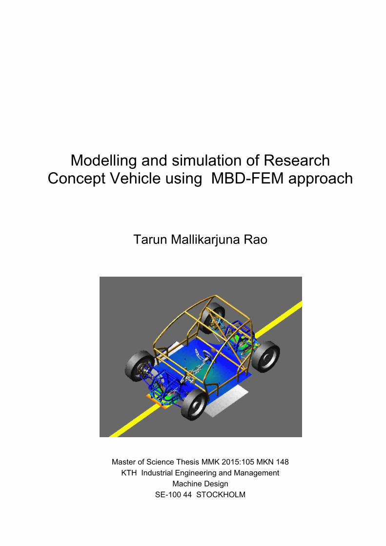
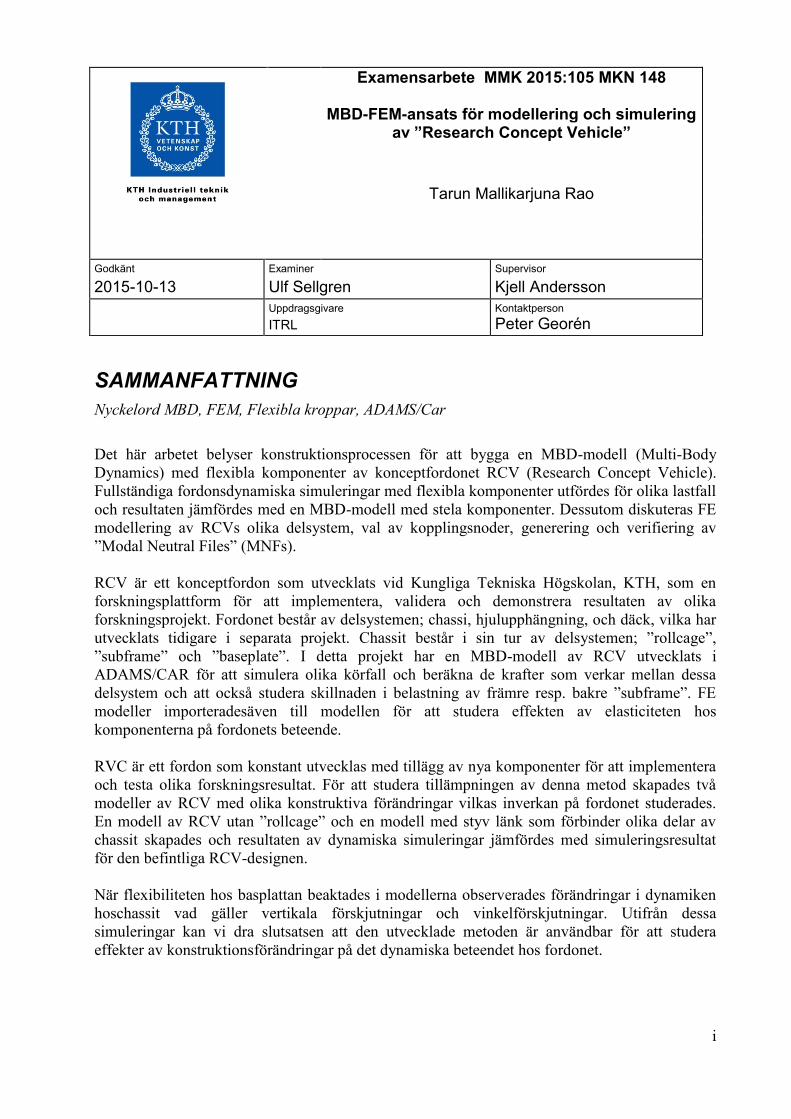
in the total mass and inertia of the complete assembly model. Similarly Figure 23 and Figure 24
give the front and rear suspension forces respectively for both the models.
28
Figure 23. Comparison of front suspension forces
Figure 24. Comparison of rear suspension forces
By comparing the results, the new model was verified to have similar dynamic characteristics as
the reference model. This model was further improved upon as specified in the next section
3.1.2. The advantage of the new body subsystem model over the existing reference model is the
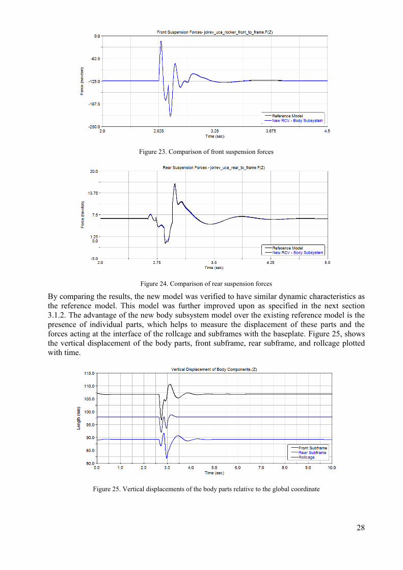
presence of individual parts, which helps to measure the displacement of these parts and the
forces acting at the interface of the rollcage and subframes with the baseplate. Figure 25, shows
the vertical displacement of the body parts, front subframe, rear subframe, and rollcage plotted
with time.
Figure 25. Vertical displacements of the body parts relative to the global coordinate
29
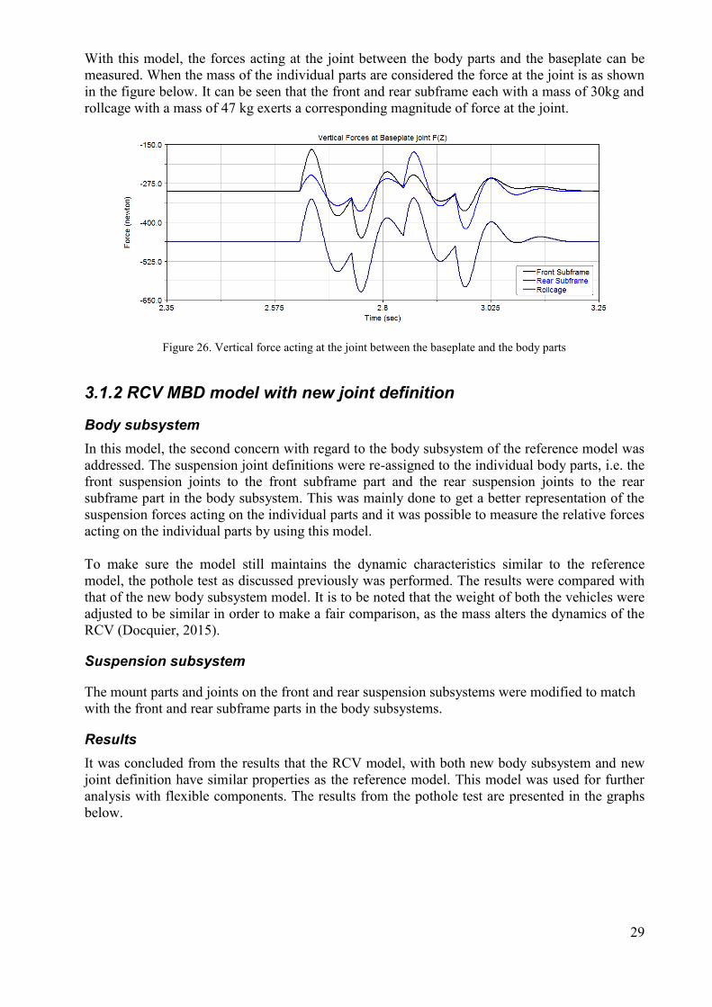
With this model, the forces acting at the joint between the body parts and the baseplate can be
measured. When the mass of the individual parts are considered the force at the joint is as shown
in the figure below. It can be seen that the front and rear subframe each with a mass of 30kg and
rollcage with a mass of 47 kg exerts a corresponding magnitude of force at the joint.
Figure 26. Vertical force acting at the joint between the baseplate and the body parts
3.1.2 RCV MBD model with new joint definition
Body subsystem
In this model, the second concern with regard to the body subsystem of the reference model was
addressed. The suspension joint definitions were re-assigned to the individual body parts, i.e. the
front suspension joints to the front subframe part and the rear suspension joints to the rear
subframe part in the body subsystem. This was mainly done to get a better representation of the
suspension forces acting on the individual parts and it was possible to measure the relative forces
acting on the individual parts by using this model.
To make sure the model still maintains the dynamic characteristics similar to the reference
model, the pothole test as discussed previously was performed. The results were compared with
that of the new body subsystem model. It is to be noted that the weight of both the vehicles were
adjusted to be similar in order to make a fair comparison, as the mass alters the dynamics of the
RCV (Docquier, 2015).
Suspension subsystem
The mount parts and joints on the front and rear suspension subsystems were modified to match
with the front and rear subframe parts in the body subsystems.
Results
It was concluded from the results that the RCV model, with both new body subsystem and new
joint definition have similar properties as the reference model. This model was used for further
analysis with flexible components. The results from the pothole test are presented in the graphs
below.

30
Figure 27. Comparison of vertical chassis displacement
Figure 28. Front suspension forces at UCA rocker to front subframe
Figure 29. Rear suspension forces at UCA rocker to rear subframe
In this model it was observed that the joint forces as shown in Figure 30 is significantly larger
than the forces in the previous model as shown in Figure 26. This increase in forces can be
attributed to the fact that the suspension joints are defined on the subframe parts and thereby
result in a better representation of forces acting at the front and rear body parts.

31
Figure 30. Forces at joint between subframes and baseplate
3.2 Flexible parts
In this section the process used for developing the flexible parts will be described for all the three
body parts of the RCV. The FE models were developed and saved as MNFs, which were verified
before being used in ADAMS/Car.
3.2.1 Baseplate
The baseplate was modelled in ANSYS APDL according to the initial design recommendations
made in baseplate design report. The base plate keypoint co-ordinates were obtained from the
CAD model and were used to create an area model in ANSYS. The baseplate was modelled as
three areas to represent the different sections. The baseplate has numerous holes in which the
inserts are bonded. Only holes where the subframes, rollcage and seats are attached to the bottom
plate were considered as attachment points for the model and the other holes were not modelled.
The composite nature of the plate was defined with the help of Shell sections using Shell 181
element.
Figure 31. Final meshed image of the bottom plate

32
Figure 32 and Figure 33 shows the element layers plot of the elements defined in section 1 and
section 2of the baseplate respectively. The orientation of the layers in these sections can be seen
in the figures. Section 2 was modelled with 2 layers more than section 1, as the original design
was performed to reduce the overall weight and increase the twist resistance in section 1. In
ANSYS his was achieved by defining layers of zero thickness.
Figure 32. Plot of element layers in section 1
Figure 33. Plot of element layers in section 2
Attachment/Interface points
Interface points define the location at which the component is connected to the rest of the system
through joints. For flexible bodies in ADAMS, interface nodes are the points at which the joints
are defined and forces act on during dynamic simulations. Spider webs of light weight and stiff
beam elements are used to model these connections. These beams help to distribute the loads
over the whole surface (Zglinska Mangorzata, Orzechowski Grzegorz, F. J. 2008).
33
Once the model is meshed, the interface point at which a joint is connected is defined by creating
a node at that attachment location. Pavel (2004) discusses few guidelines for modelling of spider
beams. It is important to define a low mass and high stiffness for the beams and in order to make
sure that the beams do not alter the natural frequencies of the original model. To verify that the
effect of spider web beams was minimal, free - free modal analysis of the model was performed
with and without the spider web beams. It was observed that model with spider web had
frequencies similar to that of the original model.
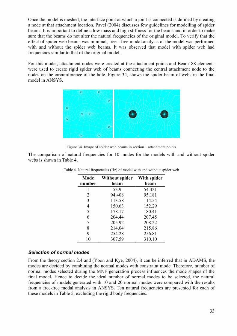
For this model, attachment nodes were created at the attachment points and Beam188 elements
were used to create rigid spider web of beams connecting the central attachment node to the
nodes on the circumference of the hole. Figure 34, shows the spider beam of webs in the final
model in ANSYS.
Figure 34. Image of spider web beams in section 1 attachment points
The comparison of natural frequencies for 10 modes for the models with and without spider
webs is shown in Table 4.
Table 4. Natural frequencies (Hz) of model with and without spider web
Mode
number
Without spider
beam
With spider
beam
1 53.9 54.421
2 94.408 95.181
3 113.58 114.54
4 150.63 152.29
5 178.17 180.41
6 204.44 207.45
7 205.92 208.22
8 214.04 215.86
9 254.28 256.81
10 307.59 310.10
Selection of normal modes
From the theory section 2.4 and (Yoon and Kye, 2004), it can be inferred that in ADAMS, the
modes are decided by combining the normal modes with constraint mode. Therefore, number of
normal modes selected during the MNF generation process influences the mode shapes of the
final model. Hence to decide the ideal number of normal modes to be selected, the natural
frequencies of models generated with 10 and 20 normal modes were compared with the results
from a free-free modal analysis in ANSYS. Ten natural frequencies are presented for each of
these models in Table 5, excluding the rigid body frequencies.

34
Table 5. Comparison of natural frequencies (Hz)
ANSYS MNF 20 normal
modes
MNF 10 normal
modes
54.42 54.44 52.78
95.18 95.22 93.86
114.54 114.84 111.05
152.29 152.79 151.15
180.41 182.19 211.98
207.45 209.81 243.80
208.22 210.92 295.12
215.86 217.93 321.78
256.81 259.77 442.01
310.10 314.13 560.16
From table 5, it can be inferred that the model with 20 normal modes correlated closely with
ANSYS results and hence was chosen as number of normal modes for MNF.
Verification of MNF
Once the final MNF was generated as discussed in section 2.6, it was verified for the following
as suggested in ANSYS help file
First the number of modes generated in the MNF was checked to see if it equalled the
sum of normal modes and constraint modes, in this case a total of 224 modes were
generated which equalled the sum of 204 (34 attachment points x 6 DOF ) constraint
modes and 20 normal modes.
The first six modes were rigid body modes and their natural frequency had low values.
The Natural frequency of first few modes were closely equal to the free-free Eigen modes
of the model as shown in table 5 for the MNF generated with 20 Normal modes
A modal analysis of the generated MNF was performed in ADAMS with all the
attachment points constrained with a fixed joint and the results were compared with that
computed in ANSYS for a fixed modal analysis. The results are shown in
Table 6.
Table 6. Comparison of natural frequencies (Hz)
ANSYS fixed modal
analysis
ADAMS fixed modal
analysis
260.54 263.33
270.33 271.41
281.74 283.04
293.56 293.79
368.21 367.15
387.99 387.14

35
3.2.2 Rollcage
The rollcage was modelled in ANSYS APDL similar to the bottom plate. The rollcage CAD
model was used to obtain the keypoint locations and the model was recreated as a line model in
ANSYS APDL. The cylindrical cross-section of the rollcage tubes was defined using beam
sections and was meshed with 3D Beam 189 elements. The hollow beam section was defined
with the CTUBE profile with inner radius of 0.018m and outer radius 0.020m according to the
CAD dimensions. The FE model was generated with 709 nodes and 360 elements. The line
element attribute was set to the beam element section defined previously.
Figure 35. Line model of the rollcage (left), meshed beam model of the rollcage (right)
In order to verify that the rollcage was modelled correctly in ANSYS APDL, the natural
frequencies of the model was compared with that of the results from a modal analysis performed
on an imported CAD model in ANSYS workbench. This method helped identify badly defined
lines and curves which were rectified before generating the MNF. The results are as shown
below. The slight difference in the frequency values can be attributed to the structural differences
in the CAD model and the simplified line model.
Table 7. Comparison of natural frequencies (Hz)
Modal analysis of CAD
model in ANSYS workbench
Modal analysis of
beam model in APDL
24.483 26.39
31.833 33.34
46.505 48.02
51.299 53.41
53.816 57.35
60.208 63.63
63.192 66.84
71.783 80.13
78.417 84.54
The rollcage body has 8 attachment points to which it connects to the bottom plate. Hence the
rollcage has a total of 48 constraint modes (8 attachment points x 6 DOFs). The modes generated
in a MNF are in accordance with the Craig-Brampton method and hence the number of normal
modes selected during the export step, influence the mode shapes in the MNF. In order to select
the number of normal modes in a way similar to the baseplate, two flexible bodies were
generated with each having 10 and 20 normal nodes. The natural frequencies of these models in

36
ADAMS were compared with the results of a free- free natural mode analysis of the model in
APDL. The results are as shown in the
Table 8. Block-Lanczos modal extraction was used in APDL to perform the modal analysis.
Lumped mass approximation was used and 20 modes were extracted. It was observed that the
flexible body extracted with 20 normal modes had natural frequencies closer to the free-free
Eigen value analysis results. Hence the body with 68 modes (48 constraint modes and 20 normal
modes) was used for the final simulation. The MNF was generated using the ADAMS macro
available in ANSYS APDL similar to the baseplate.
Table 8. Comparison of natural frequencies (Hz)
Verification of MNF
The MNF was verified in a way similar to the baseplate, the result of the fixed modal analysis of
the rollcage is shown below in Table 9. Figure 36 shows the flexible rollcage part in
ADAMS/View with fixed joints defined at its attachment points for a fixed modal analysis.
Figure 36. Flexible rollcage part in ADAMS/ View
Table 9 gives the results from the verification of the rollcage MNF.
ANSYS MNF 20 normal
modes
MNF 10 normal
modes
26.39 26.44 26.44
33.34 33.44 33.63
48.02 48.08 48.28
53.41 53.61 54.36
57.35 57.56 58.33
63.63 63.80 66.03
66.84 67.42 68.80
80.13 80.96 84.03
84.54 86.48 89.03
86.246 90.21 91.63

37
Table 9. Comparison of natural frequencies (Hz)
ANSYS fixed modal
analysis
MNF fixed modal
analysis
38.949 38.949
39.918 39.920
61.756 61.758
76.362 76.429
76.776 76.680
80.158 80.024
85.387 85.488
88.845 88.962
3.2.3 Subframe
The subframe was modelled in ANSYS APDL following the similar process as the rollcage. The
MNF was generated considering 10 attachment points at the base and with 20 normal modes.
Figure 36 shows the image of the flexible subframe part. The attachment points for the
suspension were not considered in the MNF generation for this work and need to be considered
in future work.
Figure 37. Subframe part beam model in ANSYS (left), flexible subframe part (right)
The verification of the MNF was done as mentioned for other body parts. Table 10 shows the
comparison of natural frequencies for a fixed modal analysis of the model in ANSYS to that of
the MNF in ADAMS/View.
Table 10. Verification of subframe MNF (Hz)
ANSYS fixed
modal analysis
MNF fixed
modal analysis
161.89 161.97
176.88 177.0
301.89 302.08
368.40 370.34

38
396.74 400.12
458.54 459.39
534.05 548.89
3.3 RCV MBD models
The following section presents the different RCV models developed by replacing rigid bodies
with the generated MNFs (flexible bodies). The MNFs generated in section 3.2 were imported
into ADAMS/Car to be added as flexible bodies. The RCV models with design modifications are
also discussed along with the various dynamic tests that were performed on these models.
3.3.1 RCV with flexible parts
The new MBD model and the flexible parts are integrated to form the RCV assembly with
flexible components. In ADAMS/Car the MNF file is imported and attached to the rigid bodies
through the attachment nodes defined while creating the FE models. In ADAMS, joints between
a rigid body and flexible body are defined with the help of interface parts. The flexible baseplate
and rollcage was integrated in the template mode of ADAMS/CAR. The RCV model with
flexible body parts was developed as shown in Figure 38.The rollcage, baseplate and subframes
were replaced with their respective flexible parts. This model was subjected to different load
cases as discussed later.
Figure 38. RCV with flexible body components
Another model of the RCV with flexible baseplate and rigid rollcage and subframes was built as
shown in Figure 39. The model was created to study the flexibility of the baseplate. The
subframes and rollcage were retained as rigid body to aid faster simulation and reduce memory
requirement.

39
Figure 39. RCV model with flexible baseplate
3.4 Design modifications
The RCV, due to flexibility of the baseplate was observed to undergo relative displacement of
the subframes during physical driving tests. To overcome this problem addition of rigid links
was considered and hence, models were developed to study the effect of adding a rigid link
between the rollcage and the subframe. This modification required addition of new rigid link
parts connecting the subframe and rollcage. In addition, the RCV is a research platform vehicle
which can be converted to carry cargo and might not need the rollcage. Therefore, a comparison
of models with and without a rollcage was performed. Figure 40 summarises the process used to
develop these new models. Modifications were performed on the RCV model with flexible
baseplate and rigid subframes and rollcage. These models will be discussed in detail in the
following sections.
Figure 40. Two different models that were created for the study
3.4.1 Model with rollcage and subframes joined by rigid link
In order to observe the effect of joining the rollcage and subframe together with a rigid link, two
models were developed. One model with only the front subframe and the rollcage joined by a
link (Figure 41) and the second one with both the front and rear subframes joined by a rigid link
with the rollcage (Figure 42). Figure 41, shows the model with the front subframe and rollcage
constrained by a rigid link (green part). The rigid link was created by defining a part in between

40
the rollcage and subframe and defining a fixed joint between rigid link part and the body
components. The location of the joints was defined on the respective parts.
Figure 41. RCV body subsystems with front subframe and rollcage joined by a rigid link
Figure 42, shows the model with both rear and front subframe joined by a rigid link to the
rollcage. In this case, a similar rigid part was defined between the rollcage and the rear subframe.
Figure 42. RCV model with both the front and rear subframe joined with the rollcage
Figure 43. Closer view of the rigid links in the front (left), view of rigid links in the back (right)

41
3.4.2 RCV model without rollcage
In order to study the influence of the rollcage on the RCV, a model without the rollcage was
developed. In MBD modelling terms this model was equivalent to a model without fixed joints
between a rollcage part and the baseplate part, as the mass of the component was not considered.
The larger objective of studying this model was to understand how constraining the baseplate at
different locations affects the baseplate. This study can be beneficial for design of cages for
future RCV versions. For, example a cargo model of the RCV can have a different cage with
different joint locations.
The Rollcage part was removed from the RCV model with flexible baseplate to arrive at the
model as shown in Figure 41.
Figure 44. RCV model without a rollcage
3.5 Load cases
To study the characteristics of these models dynamic tests were performed for different load
cases. The details of the tests are discussed below.
Pot-hole test
The pothole test performed on the RCV models with flexible component is similar to that
performed on the rigid models in section 3.1. In order to consider a tougher practical case a
pothole of 50mm depth was considered and the vehicle had an initial velocity of 20 km/h. Two
types of pothole road profiles were used to perform the pothole tests for different models as
shown in Figure 46.

42
Figure 45. Representation of pothole test
For the model of the RCV without rollcage the width of the pothole was varied such that only
one side of the vehicle entered the pothole. The two different pothole tests are shown in the
figure below.
Figure 46. Different pothole tests performed
Single lane change test
To measure the lateral characteristics of the model, a single lane change test was performed with
the models. This test involved the vehicle moving with an initial velocity of 20 km/h and
performing a turn with a maximum steering input of 25˚. 2D flat road profile was used for this
simulation.

43
Figure 47. Representation of single lane change test
Sinusoidal sweep steering test
This is a frequency response test. The sinusoidal sweep test involved driving the vehicle in a
straight line path while steering in a sinusoidal manner. The initial velocity of the vehicle was set
at 20 Km/h and frequencies in the range of 5Hz to 15 Hz were applied with the maximum
steering value set to 25˚.

44
4 RESULTS AND DISUSSIONS
This chapter presents the results and discussions of the dynamic simulations performed on the
RCV models.
4.1 Introduction
The RCV models were simulated for different load cased by performing standard driving tests on
ADAMS/Car. The results from the simulations are presented here along with a brief discussion.
Figure 48 shows the vehicle global axes about which the measurements were made. The axis is
oriented such that vehicle moves longitudinally in the negative X direction. The Z axis represents
the vertical axis of the vehicle and the Y axis is the lateral direction of the vehicle.
Figure 48. RCV model with the co-ordinate axes used
4.2 RCV model with flexible components
The RCV model with flexible body components was simulated to obtain results for a pothole test
with both the wheels entering the pothole as shown in Figure 49. In order to observe the effect of
flexibility of the body components, the results were compared with that of the rigid model. In
addition the results from the model with flexible baseplate, rigid subframes and rollcage were
compared and plotted. The models had similar weight and inertia properties during the
simulation tests.
The results from the simulation are presented in terms of:
1. Front and rear suspension forces
2. Vertical displacement of front and rear subframes

45
Figure 49. Representation of pothole test performed on the flexible models
The results for front and rear suspension forces and vertical displacement of baseplate were
plotted for the following three RCV models:
Table 11. Summary of the three different RCV models used
Model Baseplate Rollcage Baseplate
1 Rigid Rigid Rigid
2 Flexible Rigid Rigid
3 Flexible Flexible Flexible
Figure 50 and Figure 51 show front and rear suspension forces respectively for the three models.
It can be observed from the graph that on one hand the forces for the model with flexible parts
are closely similar when compared to the rigid body model. And on the other hand there is a
considerable difference in the suspension forces in the flexible baseplate model and the rigid
model. This change in forces can be attributed to the flexibility of the parts that were considered
in the flexible MBD models.
Figure 50. Comparison of front suspension forces

46
Figure 51. Comparison of rear suspension forces
The results from the model 1(rigid body model) and model 2(flexible baseplate model) were
used to compare the vertical displacements of the front and rear subframes. The results are
shown in Figure 52 and Figure 53 for vertical displacement of the front and rear subframe part
respectively.
Figure 52. Comparision of front subframe displacement
Figure 53. Comparison of rear subframe displacement
It can be observed from the above figures that the vertical displacement of the subframe part in
the flexible body model is different from the rigid body model. The change in displacement of
the rigid body model is smooth when compared to the flexible part and the displacements vary

47
greatly in the flexible baseplate model after the pothole impact. This can be attributed to the
flexibility of the baseplate.
4.3 RCV with flexible baseplate and parts joined by a link
The different RCV models with flexible baseplate and rigid rollcage and subframes joined
together with a rigid link as discussed in section 3.4 underwent dynamic simulations. A pothole
test and a single lane change test were performed on all the three models shown in Table 12.
Table 12. Summary of the different RCV models with rigid links used
Model Baseplate Rollcage Baseplate Rigid links
1 Flexible Rigid Rigid None
2 Flexible Rigid Rigid Front subframe and rollcage
3 Flexible Rigid Rigid Front & rear subframe and rollcage
The important observations made from the simulations are presented in terms of
1. Change in force distribution between the body components and the baseplate
2. Vertical displacements of the baseplate at different points and angular displacement of
the subframes
Figure 54 shows the joint numbers for the joints between the subframes, rollcage and the
baseplate in the RCV. The results in terms of the force and displacements were measured at these
joints and hence the graphs are represented in terms of these joint numbers.
Figure 54. Joint numbers for the front and rear subframe and the rollcage
4.3.1 Force distribution
In terms of forces it was observed that introduction of a rigid link connecting the rollcage and
subframes resulted in a change in force distribution at the joints connecting the component and
baseplate. The addition of links causes stiffening of the front and rear regions in the baseplate.
The forces acting at the joint between the subframes and baseplate and the rollcage and baseplate
are shown in the figures below.

48
The forces acting at the front subframe – baseplate joint for the RCV models with and without
links respectively.
Figure 55. Force acting at the front subframe -baseplate joint for mode with no links
Figure 56. Forces acting at the front subframe-baseplate joint for model with links in front and rear
The force at joint 3 has been significantly reduced along with a marginal decrease at joint 4. This
can be attributed to the presence of the rigid link placed close to joint 4. The force distribution at
the rollcage joints can be seen in Figure 57 and Figure 58, in the former graph it can be seen that
the forces are acting in the negative Z direction at rollcage joint 2 and 3 and in positive direction
at rollcage joint 1 and 4. The addition of the links in front and rear causes the forces at link 1
and 4 act in the negative Z direction.
Figure 57. Forces acting at the rollcage - baseplate joints for an unconstrained model

49
Figure 58. Forces acting at the rollcage - baseplate joints for model with links in front and rear
Figure 59 and Figure 60 show the forces at the joints for the rear subframe. It can be seen that the
force distribution at the rear subframe joint for the model with links in front and rear is similar to
that observed in front subframe. Joint 4 again is the joint closest to the rigid link fixture point. As
a result of these change in forces, the bending of the baseplate is affected.
Figure 59. Forces acting at the rear subframe - baseplate joints for unconstrained model
Figure 60. Forces acting at the rear subframe - baseplate joints for unconstrained model

50
4.3.2 Displacement of body components
The displacement at different points of the baseplate gives a good picture of the bending for both
static and dynamic cases. Introduction of rigid links causes the stiffening of the baseplate in the
front and back and it can be observed in the following graphs. Results from the single lane
change test (Figure 61) are discussed in this section.
Figure 61. Results from single lane change test discussed here
Figure 62 to Figure 64 shows the vertical displacement of the baseplate at points near front joint
1, rear joint 1 and rollcage joint 3 respectively. The displacement in the graphs have been
measured in the global co-ordinate and hence, the displacement value at the start time ( after the
model attains stability ) and finish time of the single lane change simulation gives the
displacement of the point from the ground for the vehicle in normal condition.
Figure 62. Comparison of vertical displacement of baseplate at front
Figure 63. Comparison of displacement of baseplate at rear

51
Figure 64. Comparison of displacement of baseplate near rollcage
It can be observed that due to the addition of rigid links in the front and the rear, there is a
decrease in initial ground clearance at the front when compared to the rear and central region of
the baseplate, where there is an increase. It is to be noted that a mass of about 350 kg is acting
close to rear of the baseplate. This change can be caused due to the stiffening of the front and
rear region of the baseplate by addition of rigid links, which is restricting the bending of the plate
around these regions. At the same time the mass acting near the rear is causing the baseplate to
bend downwards.
Figure 65 shows the vertical displacements of the body components form the model with rigid
links in front and rear. The rollcage point 3 curve has a larger displacement as it is a point at a
farther distance from the centre when compared to the other points.
Figure 65. Vertical displacement of body components for model constrained in front and rear
The angular displacement of the body subsystems gives a better idea of the influence of the rigid
links as shown in Figure 66 to Figure 69 shows the angular displacement PHI for the body
components - rollcage, front and rear subframe for the models with and without link. These
displacements were chosen for a better representation of the effect of the links.
Figure 66 shows the angular displacement (PHI) for the model without any links. It can be seen
that rear subframe has the maximum angular displacement, followed by the rollcage and the
front subframe.
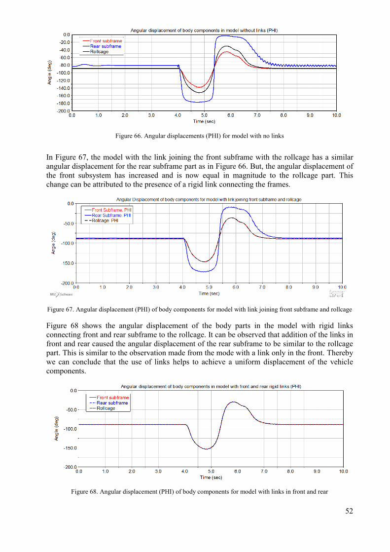
52
Figure 66. Angular displacements (PHI) for model with no links
In Figure 67, the model with the link joining the front subframe with the rollcage has a similar
angular displacement for the rear subframe part as in Figure 66. But, the angular displacement of
the front subsystem has increased and is now equal in magnitude to the rollcage part. This
change can be attributed to the presence of a rigid link connecting the frames.
Figure 67. Angular displacement (PHI) of body components for model with link joining front subframe and rollcage
Figure 68 shows the angular displacement of the body parts in the model with rigid links
connecting front and rear subframe to the rollcage. It can be observed that addition of the links in
front and rear caused the angular displacement of the rear subframe to be similar to the rollcage
part. This is similar to the observation made from the mode with a link only in the front. Thereby
we can conclude that the use of links helps to achieve a uniform displacement of the vehicle
components.
Figure 68. Angular displacement (PHI) of body components for model with links in front and rear

53
Figure 69 gives a comparison of the angular displacement of body components in models with
and without rigid links. The constrained model in the graph refers to the model with rigid links in
the front and rear.
Figure 69. Comparison of angular displacement (PHI) for model without links and with links in front and rear
4.4 RCV without rollcage
The results for single wheel pothole test as shown in Figure 70 were conducted on the RCV
models with a flexible plate with and without rollcage. The results from the simulation are
presented below. The masses of both the models were kept similar.
Figure 70. Representation of pothole test conducted for the model without rollcage
Figure 71 shows the comparison of vertical displacement at front joint 1. It was observed that the
vertical displacement of the model without rollcage is relatively higher while entering the bump.
Yet, the difference in displacements of two models is about only 6 to 10 mm, similar results were
observed at the other points of the baseplate.

54
Figure 71. Comparison of vertical displacement at front joint1
The angular displacement at point 3 of the rollcage is shown in the following Figure 72. Larger
angular displacement was observed in the model with no rollcage when compared to the model
with rollcage joints. It can also be observed that the model with a rollcage reaches a stable
condition faster when compared to the model without a rollcage, as observed by the peaks
occurring between 6 to 7 seconds in the simulation. From this it can be inferred that the model
with a rollcage joint is relatively more stable compared to the model without any rollcage joints.
Figure 72. Comparision of angular displacement (PHI) at roll joint 3
Result from sinusoidal sweep steer test
A swept sine test was performed on the two models and the comparison of angular displacement
at rollcage joint 3 is as show in Figure 73. It can be seen from the figure that the model without a
rollcage shown in the blue has higher amplitude when compared to the model with a rollcage,
which is undesirable from the context of stability and comfort.
Figure 73. Comparison of angular displacement (theta) at rollcage joint 3

55
5 CONCLUSIONS
The goals set to achieve in the problem statement section was addressed as discussed below.
How to develop a MBD model to determine the forces acting on the different RCV
subsystems ?
o This was achieved in this work as shown in section 3.1. Section 3.1.1 and 3.1.2
discussed the the two rigid body models that were developed and verified, the model
helped measure the forces acting at the interface of the body components and
considered the suspension forces acting on the subframe parts. Later in section 3.3,
models of the RCV with flexible baseplate with multiple joints were developed.
How to model flexible bodies of the RCV sub-systems for multibody simulations ?
o Flexibe bodies of the RCV were developed as discussed in section 3.2. The modelling
of all the three components- baseplate, rollcage and subframe were discussed.The
bodies were modelled in FEM Software and a MNF file was generated. Based on the
theory discussed in section 2.4, the models’ MNF file was generated by selecting the
desired number of normal modes for each component.The MNF files were verified
before being used in ADAMS.
Can the vehicle model be used to consider the flexibility of the bottom plate ?
o Yes, with the RCV model with flexible baseplate, it was possible to consider the
flexibility of the baseplate. As discussed in section 4.2 various dynamic simulations
were perfomed on the models and the displacements at different locations of the plate
were considered to observe the bending of the plate.
How does connecting the rollcage and sub frames together influence the behaviour of the
vehicle ?
o As discussed in section 4.3,the addition of links to join the rollcage and sub-frame is
desirable to achieve uniform motion of all body components, as the links helped to
stiffen the vehicle and achieve a more uniform angular displacement of the
components throughout the maneouver.The addition of links should be decided based
on the application of the RCV, as high forces can act at the rigid link joints.
How does the rollcage affect the dynamic behaviour of the vehicle ?
o It was observed that the absence of joints holding together the central section of the
baseplate didn’t vary the results in terms of vertical displacements. But, the results
from the sinusoidal swept steer test showed high amplitudes for the model without
rollcage which was undesirable. Hence, addition of joints to constrain the central
section is desirable.

56
6 RECOMMENDATIONS AND FUTURE WORK
This chapter contains the recommendations of more detailed development and proposed future
work.
6.1 Recommendations
1. Given the favourable results from the simulations performed in this work in regard to
addition of rigid links between the body components, it would be interesting to optimize
the location of the joints by performing some design simulations. Ultimately an
experimental verification is to be performed to check the results of adding rigid links.
2. Holding together the central section of the baseplate with a rollcage joints helps in
reducing the amplitude of flexing in the plate. The form or mass of the rollcage was not
taken into consideration in this work and could influence the results. Hence, for future
versions of the RCV, it is possible to have rollcages of different shapes and for different
purpose, helping to reduce the baseplate bending along the edges.
6.2 Future work
The RCV is a vehicle under development and is constantly changing as new components are
added to test new research results. The current model can be improved upon to achieve a more
accurate representation of the RCV as changes are performed on the vehicle. The following steps
explain briefly on the future work that can be performed to improve this model.
1. The flexible bodies can be incorporated in the co-simulation controlled model and
simulations can be performed to verify and validate the model with experimental results.
2. The mass and inertia of the passengers can be considered at the location of the seats to
further improve the model. An accurate representation of the mass acting on the flexible
baseplate can be achieved by defining the passenger loads as separate parts. Karanam,
Chatterjee and Ghosal (2011), modelled a flexible three wheeler frame structure
considering the passengers.
3. The flexible components can be used to generate the stress and strain plots using modal
stress recovery method. This can help locate the regions in the body subsystem where the
stress is maximum.
4. The trans-shear stiffness coefficient was not included while modelling the baseplate. The
effect of this property needs to be studied and considered in the future models.
5. Developing a powertrain subsystem model for the RCV will be beneficial to continue the
work in its current stage, without the need for co-simulation.

57
REFERENCES
ADAMS Flex, 2002, MSC.Software Corporation
ADAMS/Car, Getting Started with ADAMS/Car 2013,MSC.Software Corporation
Gang, X., Yan, Z., Fanli, Z., &Liping, C. (2012). Modelling and Simulation of the Coupled
Rigid-flexible Multibody Systems in MWorks, 405-416. Retrieved from
http://www.ep.liu.se/ecp_article/index.en.aspx?issue=76;article=42
Gupta, S., Bardhan, A., Khanger, R., and Matharu, R., 2011 "Front Suspension Modeling Using
an Integrated FEM - Multi Body Approach," SAE Technical Paper 2011-28-0078,
doi:10.4271/2011-28-0078.
Karanam, V. M., Chatterjee, A., &Ghosal, A. (2011). Procedural aspects of modeling the
dynamics of a three wheeled vehicle using ADAMS-CAR.Unpublished Public License.Retrieved
from http://eprints.iisc.ernet.in/42809/\nhttp://eprints.iisc.ernet.in/42809/4/updated_version.pdf
Martin Kieltsch / Berechnungsmethoden, Full vehicle models at VW, International ADAMS
Users Conference 2000
Sellgren, U., 2003, “Component Mode Synthesis. A Method for Efficient Dynamic Simulation of
Complex Technical Systems,” Technical Report, Department of Machine Design, The Royal
Institute of Technology (KTH), Stockholm, Sweden.
Shahidi, B., Stuhec, U., Shahidi, B., Tavakkoli, S. et al., 2006,"System Level Durability
Engineering in CAE," SAE Technical Paper 2006-01-1981, 2006, doi: 10.4271/2006-01-1981.
Steve Pilz, 2008, Page 40-42,ANSYS Advantage • Volume II, Issue 4,
ZglinskaMangorzata, OrzechowskiGrzegorz, F. J. (2008). DYNAMICAL ANALYSIS OF THE
DEFORMABLE POWER TRANSMISSION MECHANISM USING MIXED FEM AND MBS
METHOD. Journal of KONES Powertrain and Transport, 15.
Kakria, Sahil, and Daljeet Singh. 2015. CAE Analysis, Optimization and Fabrication of Formula
SAE Vehicle Structure.
Novotny P, 2004, Cranktrain Dynamics simulation-Central module of virtual
engine,BrnoUniversity of Technology.
Yoon, J. and Kye, K., 2004,"Suspension Abuse Test Simulation using Modal Stress Recovery,"
SAE Technical Paper 2004-01-0776, doi:10.4271/2004-01-0776.
Kiviniem T., Holopainen T., 1998, “Modelling of flexible members for simulation of vehicle
dynamics”, Espoo 29.12.1999
Docquier Q, 2015, “Modelling of Flexible Multibody Systems: Application to Road Vehicle
with Flexible Chassis”, Universite catholique de Louvain
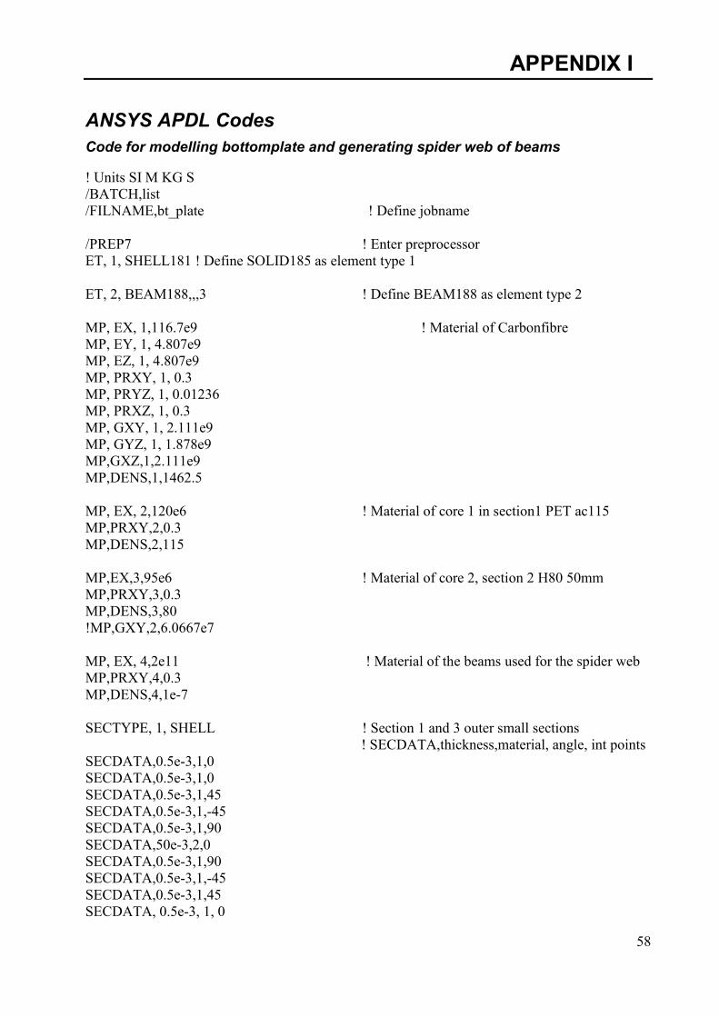
58
APPENDIX I
ANSYS APDL Codes
Code for modelling bottomplate and generating spider web of beams
! Units SI M KG S
/BATCH,list
/FILNAME,bt_plate ! Define jobname
/PREP7 ! Enter preprocessor
ET, 1, SHELL181 ! Define SOLID185 as element type 1
ET, 2, BEAM188,,,3 ! Define BEAM188 as element type 2
MP, EX, 1,116.7e9 ! Material of Carbonfibre
MP, EY, 1, 4.807e9
MP, EZ, 1, 4.807e9
MP, PRXY, 1, 0.3
MP, PRYZ, 1, 0.01236
MP, PRXZ, 1, 0.3
MP, GXY, 1, 2.111e9
MP, GYZ, 1, 1.878e9
MP,GXZ,1,2.111e9
MP,DENS,1,1462.5
MP, EX, 2,120e6 ! Material of core 1 in section1 PET ac115
MP,PRXY,2,0.3
MP,DENS,2,115
MP,EX,3,95e6 ! Material of core 2, section 2 H80 50mm
MP,PRXY,3,0.3
MP,DENS,3,80
!MP,GXY,2,6.0667e7
MP, EX, 4,2e11 ! Material of the beams used for the spider web
MP,PRXY,4,0.3
MP,DENS,4,1e-7
SECTYPE, 1, SHELL ! Section 1 and 3 outer small sections
! SECDATA,thickness,material, angle, int points
SECDATA,0.5e-3,1,0
SECDATA,0.5e-3,1,0
SECDATA,0.5e-3,1,45
SECDATA,0.5e-3,1,-45
SECDATA,0.5e-3,1,90
SECDATA,50e-3,2,0
SECDATA,0.5e-3,1,90
SECDATA,0.5e-3,1,-45
SECDATA,0.5e-3,1,45
SECDATA, 0.5e-3, 1, 0

59
SECDATA, 0.5e-3, 1, 0
SECTYPE, 2, SHELL
SECDATA,0.5e-3,1,0
SECDATA,0.5e-3,1,0
SECDATA,0.5e-3,1,45
SECDATA,0.5e-3,1,-45
SECDATA,0,1,0
SECDATA,50e-3,3,0
SECDATA,0,1,0
SECDATA,0.5e-3,1,-45
SECDATA,0.5e-3,1,45
SECDATA, 0.5e-3, 1, 0
SECDATA, 0.5e-3, 1, 0
SECTYPE,3,BEAM,ASEC ! Beam properties for spider web
!SECDATA,0.0009,5e-6,,5e-6,,10,,,857.160,857.160
SECDATA,7.8528e-5,49067e-8,,49067e-8,,10,,,857.16,857.16
K,1,-1.305,0.26720,0 ! Keypoint locations
K,2,-0.855,0.26720,0
K,3,-0.855,0.41720,0
K,4,-0.74950,0.31057,0
K,5,-0.66597,0.44190,0
K,6,-0.99566,0.55938,0
K,7,-0.630,0.650,0
K,8,-1.250,0.650,0
K,9,-0.630,0.75,0
K,10,-1.305,-0.26720,0
K,11,-0.855,-0.26720,0
K,12,-0.855,-0.41720,0
K,13,-0.74950,-0.31057,0
K,14,-0.66597,-0.44190,0
K,15,-0.99566,-0.55938,0
K,16,-0.630,-0.650,0
K,17,-1.250,-0.650,0
K,18,-0.630,-0.75,0
K,19,-0.6,0.75,0
K,20,-0.6,-0.75,0
K,21,1.305,0.26720,0
K,22,0.855,0.26720,0
K,23,0.855,0.41720,0
K,24,0.74950,0.31057,0
K,25,0.66597,0.44190,0
K,26,0.99566,0.55938,0
K,27,0.630,0.650,0
K,28,1.250,0.650,0
K,29,0.630,0.75,0
K,30,1.305,-0.26720,0
K,31,0.855,-0.26720,0
K,32,0.855,-0.41720,0

60
K,33,0.74950,-0.31057,0
K,34,0.66597,-0.44190,0
K,35,0.99566,-0.55938,0
K,36,0.630,-0.650,0
K,37,1.250,-0.650,0
K,38,0.630,-0.75,0
K,39,0.6,0.75,0
K,40,0.6,-0.75,0
L,1,2 ! Connecting keypoints with lines
Larc,2,4,3,0.15
Larc,4,5,6,0.35
Larc,5,7,8,0.62
L,7,9
L,18,16
Larc,16,14,17,0.62
Larc,14,13,12,0.35
Larc,13,11,12,0.15
L,11,10
L,10,1
L,21,22
Larc,22,24,23,0.15
Larc,24,25,26,0.35
Larc,25,27,28,0.62
L,27,29
L,38,36
Larc,36,34,37,0.62
Larc,33,34,32,0.35
Larc,31,33,32,0.15
L,30,31
L,21,30
!L,7,16
L,18,20
L,20,40
L,40,38
L,9,19
L,19,39
L,39,29
L,39,40
L,19,20
AL,P
!------BREAK----
CYL4,-1.253,.1449,.0105 ! Modelling holes on the plate surface
CYL4,-1.142,.241,.0105
CYL4,-.942,.241,.0105
CYL4,-.7892,.0624,.0105
CYL4,-.7892,-.0624,.0105
CYL4,-.942,-.241, .0105
CYL4,-1.142,-.241,.0105

61
CYL4,-1.253,-.1449,.0105
CYL4,-1.0405, 0, .0105
CYL4,-.9595, 0, .0105
CYL4, .942,.241,.0105
CYL4, 1.142,.241,.0105
CYL4, 1.253,.144,.0105
CYL4, 1.253,-.1449,.0105
CYL4, 1.142,-.241,.0105
CYL4, .942,-.241,.0105
CYL4, .789,-.0624,.0105
CYL4, .789,.0624,.0105
CYL4, .959,0,.0105
CYL4, 1.0405,0,.0105
Cyl4,-0.530, 0.7,0.0105
Cyl4,-0.280, 0.70, 0.0105
Cyl4, 0.280, 0.7, 0.0105
Cyl4,0.530,0.7,0.0105
Cyl4,0,0.475,0.0105
Cyl4,-0.22250,0.080,0.0105
Cyl4,0.22250,0.080,0.0105
Cyl4,-0.530,-0.7,0.0105
Cyl4,-0.280,-0.70,0.0105
Cyl4,0.280,-0.7,0.0105
Cyl4,0.530,-0.7,0.0105
Cyl4,0.575,-0.475,0.0105
Cyl4,0,-0.475,0.0105
Cyl4,-0.22250,-0.080,0.0105
Cyl4,0.22250,-0.080,0.0105
! The additional surfaces were deleted manually and the model was meshed.
! Assigning attachment nodes at attachment locations
*GET,totaln,node,,count
N,totaln+1,-1.253 ,.1449
N, totaln+2,-1.142,.241
N, totaln+3,-.942,.241
N, totaln+4,-.7892,.0624
N, totaln+5,-.7892,-.0624
N, totaln+6,-.942,-.241
N, totaln+7,-1.142,-.241
N, totaln+8,-1.253,-.1449
N, totaln+9,-1.0405,0,
N, totaln+10,-.9595,0
N, totaln+11,.942,.241
N, totaln+12,1.142,.241
N, totaln+13,1.253,.144
N, totaln+14,1.253,-.1449
N, totaln+15,1.142,-.241
N, totaln+16,.942,-.241
N, totaln+17,.789,-.0624
N, totaln+18,.789,.0624
N, totaln+19,.959,0

62
N, totaln+20,1.0405,0
N, totaln+21,-0.530,0.7
N, totaln+22,-0.530,-0.7
N, totaln+23,0.530,0.7
N, totaln+24,0.530,-0.7
N, totaln+25,-0.280,0.7
N, totaln+26,-0.280,-0.7
N, totaln+27,0.280,0.7
N, totaln+28,0.280,-0.7
N, totaln+29,-0.22250,-0.080
N, totaln+30,0.22250,-0.080
N, totaln+31,-0.22250,0.080
N, totaln+32,0.22250,0.080
N, totaln+33,0,0.475
N, totaln+34,0,-0.475
! Generating Spider Web of beams
*SET, kk, 0
*Do, kk, totaln+1, totaln+34
NWPAVE,kk ! Set working plane to interface point 1
WPSTYL,,,,,, 1 ! Set working plane type to cylindrical
CSYS, 4 ! Activate working plane
NSEL, S, LOC, X,.0105 ! Select nodes on cylindrical hole
NSEL,A,,,kk ! Also select interface node
*GET,nmin,node,,num,min ! Assigns minimum node number to nmin
*GET,nnum,node,,count !similarly assigns total nodes to nnum
*SET, jj, 0
TYPE, 2 ! Defines element type 2
MAT, 4 ! Defines material as 4
SECNUM, 3 ! Defines section number as 3
*DO, jj, 1, nnum-1 ! Subtracting the centre node from the node count
E,kk ,nmin! Defining elements by node connectivity to the minimum node in the hole
NSEL,u,,,nmin ! Unselects that node
*GET,nmin,node,,num,min !gets new minimum node
*ENDDO
*ENDDO
ALLs
Code for modelling rollcage

63
/PREP7 ! Enter preprocessor
MP, EX, 1,2e11 ! Material of rollcage structure:steel
MP,PRXY,1,0.3
MP,DENS,1,7850
ET,1,BEAM189 ! Define BEAM189 as element type 1
!SECTYPE = Beam – CTUB, The beam type and diameters were entered manually
K,1,-0.530,-0.7,0.037 ! Keypoint locations
K,2,-0.53,-0.7,0.094
K,3,-0.650,-0.7,0.094
K,4,-0.53409,-0.7,0.12506
K,5,-0.55346,-0.70,0.2
K,46,-0.64725,-0.7,0.550
K,47,-0.65867,-0.7,0.590
K,48,0.07850,-0.58180,1.16875
K,49,0.64725,-0.7,0.550
K,50,0.55345,-0.7,0.2
K,51,0.72226,-0.64118,0.82995
K,52,0.53120,-0.7,0.11227
K,6,-0.66671,-0.7,0.620
K,7,-0.55187,-0.68369,0.65077
K,8,-0.63422,-0.69152,0.73771
K,9,-0.56267,-0.67960,0.80655
K,10,0.46665,-0.58181,-0.28016
K,11,0.81487,-0.484,1.17558
K,12,0.82142,-0.40370,1.20004
K,13,0.79758,-0.53525,1.11106
K,14,0.78519,-0.40370,1.06481
K,15,0.68643,-0.69156,0.69625
K,16,0.67404,-0.560,0.65
K,17,0.67404,-0.7,0.650
K,18,0.53477,-0.7,0.13023
K,19,0.670,-0.7,0.094
K,20,0.530,-0.7,0.094
K,21,0.530,-0.7,0.037
K,22,-0.58096,-0.7,0.3
K,23,-0.58096,0.7,0.3
K,26,0.82142,0,1.20004
K,27,-0.530,0.7,0.037
K,28,-0.53,0.7,0.094
K,29,-0.650,0.7,0.094
K,30,-0.53409,0.7,0.12506
K,31,-0.66671,0.7,0.620
K,32,-0.55187,0.68369,0.65077
K,33,-0.63422,0.69152,0.73771
K,34,-0.56267,0.67960,0.80655
K,35,0.46665,0.58181,-0.28016
K,36,0.81487,0.484,1.17558
K,37,0.82142,0.40370,1.20004

64
K,38,0.79758,0.53525,1.11106
K,84,0.78519,0.40370,1.06481
K,39,0.68643,0.69156,0.69625
K,40,0.67404,0.560,0.65
K,41,0.67404,0.7,0.650
K,42,0.53477,0.7,0.13023
K,43,0.670,0.7,0.094
K,44,0.530,0.7,0.094
K,45,0.530,0.7,0.037
K,53,-0.55346,0.70,0.2
K,54,-0.64725,0.7,0.550
K,55,-0.65867,0.7,0.590
K,56,0.07850,0.58180,1.16875
K,57,0.64725,0.7,0.550
K,58,0.55345,0.7,0.2
K,59,0.72226,0.64118,0.82995
K,60,0.53120,0.7,0.11227
L,1,2 ! Connecting keypoints with Lines
Larc,2,4,3,0.120
L,4,5
L,5,22
L,22,46
L,46,47
L,47,6
Larc,6,8,7,0.120
L,8,9
L,27,28
Larc,9,48,10,1.5
Larc,11,48,10,1.5
Larc,13,11,14,0.140
Larc,12,11,14,0.140
L,12,26
L,26,37
L,51,13
L,15,51
Larc,15,17,16,0.140
L,17,49
L,49,50
L,50,18
Larc,18,52,19,0.140
Larc,52,20,19,0.140
L,20,21
L,27,28
Larc,28,30,29
L,12,26
Larc,28,30,29,0.120
L,30,53
L,53,23
L,23,54
L,54,55
L,55,31
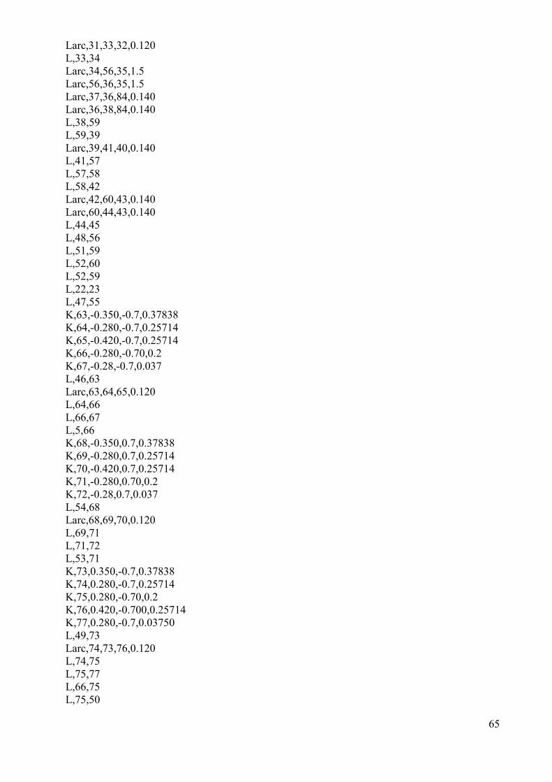
65
Larc,31,33,32,0.120
L,33,34
Larc,34,56,35,1.5
Larc,56,36,35,1.5
Larc,37,36,84,0.140
Larc,36,38,84,0.140
L,38,59
L,59,39
Larc,39,41,40,0.140
L,41,57
L,57,58
L,58,42
Larc,42,60,43,0.140
Larc,60,44,43,0.140
L,44,45
L,48,56
L,51,59
L,52,60
L,52,59
L,22,23
L,47,55
K,63,-0.350,-0.7,0.37838
K,64,-0.280,-0.7,0.25714
K,65,-0.420,-0.7,0.25714
K,66,-0.280,-0.70,0.2
K,67,-0.28,-0.7,0.037
L,46,63
Larc,63,64,65,0.120
L,64,66
L,66,67
L,5,66
K,68,-0.350,0.7,0.37838
K,69,-0.280,0.7,0.25714
K,70,-0.420,0.7,0.25714
K,71,-0.280,0.70,0.2
K,72,-0.28,0.7,0.037
L,54,68
Larc,68,69,70,0.120
L,69,71
L,71,72
L,53,71
K,73,0.350,-0.7,0.37838
K,74,0.280,-0.7,0.25714
K,75,0.280,-0.70,0.2
K,76,0.420,-0.700,0.25714
K,77,0.280,-0.7,0.03750
L,49,73
Larc,74,73,76,0.120
L,74,75
L,75,77
L,66,75
L,75,50

66
K,78,0.350,0.7,0.37838
K,79,0.280,0.7,0.25714
K,80,0.280,0.70,0.2
K,81,0.420,0.700,0.25714
K,82,0.280,0.7,0.03750
L,57,78
Larc,78,79,81,0.120
L,79,80
L,80,82
L,71,80
L,80,58
Code for modelling subframe
/PREP7 ! Enter preprocessor
MP, EX, 1,2e11 ! Material of subframe structure: steel
MP,PRXY,1,0.3
MP,DENS,1,7850
ET,1,BEAM189 ! Define BEAM189 as element type 1
!SECTYPE,1,Beam,CTUBE
!Secdata,1,0.015875,0.013325
!Sectype,2,beam,ctube
!Secdata,2,0.01111,0.0049
K,1,0.127,0.241,0.1585
K,2,0.1,.241,.1585
K,3,0.0581,.241,.1585
K,4,-0.1,0.241,0.1585
K,5,-0.1419,0.241,0.1585
K,6,-0.173,0.241,0.1585
K,7,-.173,.161,.1585
K,8,-.253,.161,.1585
K,9,-.253,.1449,.1585
K,10,-.253,.0948,.1585
K,11,-.253,.0303,.1585
K,12,-.253,-.0303,.1585
K,13,-.253,-.0948,.1585
K,14,-.253,-.1449,.1585
K,15,-.253,-.161,.1585
K,16,-.173,-.161,.1585
K,17,-.173,-.241,.1585
K,18,-.1419,-.241,.1585
K,19,-.1,-.241,.1585
K,20,.0581,-.241,.1585
K,21,.1,-.241,.1585
K,22,.127,-.241,0.1585
K,23,.0581,-.241,.135

67
K,24,-0.1419,-0.241,.135
K,25,-0.253,-0.1449,.135
K,26,-.253,.1449,.135
K,27,-.1419,.241,.135
K,28,0.0581,.241,.135
K,29,-0.05125,-0.280,0.291
K,30,-0.1,-0.280,0.291
K,31,-0.173,-0.280,0.291
K,32,-0.173,-0.200,0.291
K,33,-0.253,-0.200,0.291
K,34,-0.253,-0.1798,0.291
K,35,-0.253,-0.1219,0.291
K,36,-0.253,0,0.291
K,37,-0.253,0.1219,0.291
K,38,-0.253,0.1798,0.291
k,39,-0.253,0.200,0.291
k,40,-0.173,0.200,0.291
k,41,-0.173,0.280,0.291
k,42,-0.1,0.280,0.291
K,43,-0.05125,0.280,0.291
K,44,0.1,-0.280,0.291
K,45,0.13080,-0.280,0.291
K,46,0.13080,-0.200,0.291
K,47,0.21080,-0.200,0.291
K,48,0.21080,-0.17730,0.291
K,49,0.21080,0,0.291
K,50,0.2108,0.17730,0.291
K,51,0.21080,0.200,0.291
K,52,0.13080,0.200,0.291
K,53,0.13080,0.280,0.291
K,54,0.1,0.280,0.291
K,55,-0.1,-0.25022,0.18983
K,56,0.1,-0.27078,0.25967
K,57,-0.1,0.25022,0.18983
K,58,0.100,0.27078,0.25967
L,22,21
L,21,20
L,20,19
L,19,18
L,18,17
LARC, 17, 15, 16, .080
L, 15, 14
L, 14, 13
L, 13, 12
L, 12, 11
L, 11, 10
L, 10, 9
L, 9, 8
LARC, 8, 6, 7, .080
L, 6, 5
L, 5, 4
L, 3, 4

68
L, 3, 2
L, 2, 1
L, 20, 23
L, 18, 24
L, 14, 25
L, 9, 26
L, 5, 27
L, 3, 28
L,29,30
L,30,31
Larc,31,33,32,0.080
L,33,34
L,34,35
L,35,36
L,36,37
L,37,38
L,38,39
Larc,39,41,40,0.080
L,41,42
L,42,43
L,10,37
L,13,35
L,19,55
L,55,30
L,4,57
L,57,42
L,29,44
L,44,45
L,47,48
L,48,49
L,49,50
L,50,51
L,54,53
L,53,43
Larc,45,47,46,0.080
Larc,51,53,52,0.080
L,21,56
L,56,44
L,2,58
L,58,54
L,55,56
L,57,58
K,59,0.21080,-0.15520,0.21591
K,60,0.21080,-0.07846,0.23850
K,61,0.21080,-0.07846,0.15850
K,62,0.21080,-0.06240,0.15850
K,63,0.21080,-0.0303,0.15850
K,64,0.21080,0,0.15850
K,65,0.21080,0.0303,0.15850
K,66,0.21080,0.06240,0.15850
K,67,0.21080,0.07846,0.15850
K,68,0.21080,0.07846,0.23850

69
K,69,0.21080,0.15520,0.21591
K,70,0.21080,-0.0624,0.135
K,71,0.21080,0.0624,0.135
L,48,59
L,61,62
L,62,70
L,62,63
L,63,64
L,64,65
L,65,66
L,66,67
L,66,71
L,69,50
LARC,59,61,60,0.080
LARC,69,67,68,0.080
K,74,0.21080,-0.17730,0.37190
K,75,0.20330, -0.17730,0.40571
K,76,0.13080, -0.17730,0.37190
K,77,0.13028, -0.17730,0.56232
K,78,0.04388, -0.17730,0.60729
K,79,0.05777, -0.17730,0.52851
K,80,-0.128, -0.17730,0.57698
K,81,-0.18661, -0.17730,0.53201
K,82,-0.114, -0.17730,0.49820
K,83,-0.24550, -0.17730,0.40571
K,84,-0.253, -0.17730,0.37190
K,85,-0.173, -0.17730,0.37190
K,86,0.21080, 0.17730,0.37190
K,87,0.20330, 0.17730,0.40571
K,88,0.13080, 0.17730,0.37190
K,89,0.13028, 0.17730,0.56232
K,90,0.04388, 0.17730,0.60729
K,91,0.05777, 0.17730,0.52851
K,92,-0.128, 0.17730,0.57698
K,93,-0.18661, 0.17730,0.53201
K,94,-0.114, 0.17730,0.49820
K,95,-0.24550, 0.17730,0.40571
K,96,-0.253, 0.17730,0.37190
K,97,-0.173, 0.17730,0.37190
K,98,-0.25110,0.17730,0.38922
K,99,-0.16281,0.17730,0.56167
K,100,0.09471,0.17730,0.59947
K,101,0.20890,0.17730,0.38922
K,102,-0.25110,-0.17730,0.38922
K,103,-0.16281,-0.17730,0.56167
K,104,0.09471,-0.17730,0.59947
K,105,0.20890,-0.17730,0.38922
Larc,84,102,85,0.080
Larc,102,83,85,0.080
Larc,81,103,82,0.080
Larc,103,80,82,0.080
Larc,78,104,79,0.080

70
Larc,77,104,79,0.080
Larc,75,105,76,0.080
Larc,105,74,76,0.080
L,75,77
L,80,78
l,81,83
Larc,96,98,97,0.080
Larc,98,95,97,0.080
Larc,92,99,94,0.08
Larc,99,93,94,0.080
Larc,89,100,91,0.080
Larc,100,90,91,0.080
Larc,87,101,88,0.080
Larc,101,86,88,0.080
L,93,95
L,90,92
L,89,87
L,101,105
L,104,100
L,103,99
L,102,98
L,38,96
L,84,34
L,48,74
L,86,50
K,106, 0.041,0.03030,0.15850
K,107, 0.041,-0.03030,0.15850
K,108, -0.041,0.03030,0.15850
K,109, -0.041,-0.03030,0.15850
K,110,0.041,0,0.15850
K,111,-0.041,0,0.15850
K,112, -0.041,0,0.135
K,113, 0.041,0,0.135
L,111,112
L,110,113
L,108,111
L,111,109
L,106,110
L,110,107
L,108,106
L,109,107
L,107,63
L,109,12
L,108,11
L,106,65