1

Modelling Breaks in Consumer Expenditure:

Evidence for Argentina

HILDEGART A. AHUMADA† AND MARIA LORENA GAREGNANI‡

† Di Tella University, Miñones 2159 (1428), Buenos Aires, Argentina E-mail: hahumada@utdt.edu

‡Central Bank of Argentina, Reconquista 266, 7mo. Edificio Central, 2703 (1003). Buenos Aires, Argentina and University of La Plata*

E-mail: lgaregnani@bcra.gov.ar

July 2011

Abstract This paper shows how parameter non-constancy can be seen as informative about a different aggregate consumer behaviour resulting from an economic regime change. We have developed for Argentina (1980-2010) an Equilibrium-Correction Model whose parameter estimates are used to test liquidity constraints vs. wealth effects. Liquidity constraints are found to be regime specific as they characterize Argentine consumption during the period starting soon after the abandonment of a convertibility regime takes place and last for 14 quarters until consumption reaches the highest level since 1980. The concept of co-breaking is also discussed. Keywords: Equilibrium-Correction – Wealth-Effects – Liquidity-Constraints – Co-breaking

JEL: C32, E21

*We thank Neil Ericsson, Daniel Heymann, Fernando Navajas and Alfredo Navarro for many insightful discussions. The views expressed herein are solely our own and should not be interpreted as those of the Central Bank of Argentina.

2

1. Introduction Empirical modellers frequently face structural breaks and different policy regimes but these shifts are pervasive in economies subject to macroeconomic instability, where even consumption-saving decisions seem not easy for economic agents. Modelling aggregate consumer behaviour in such cases would be even more difficult as parameter changes have usually been considered as a main obstacle for both “the solved-out consumption function” and “the Euler Equation-Generalized Method of Moments (GMM)” approaches, the most frequently followed empirical methodologies. The instability of deep parameters describing consumer preferences at aggregate levels is often pointed out in the applied literature (Favero, 2001; Ahumada and Garegnani, 2004, among others). At the same time, the theory of forecasting has found that equilibrium-mean changes are often detected in “Error Correction” models, which are usually formulated following the other approach. “Error Correction” models have been consequently renamed as “Equilibrium Correction” since such equilibrium may be actually wrong when the “true” one has shifted (Clements and Hendry, 1999).

Based on an Equilibrium Correction (EC) model of Argentina´s consumer expenditure, this paper is aimed at showing how parameter non-constancy can be seen as informative about a different aggregate behaviour resulting from changes in economic regimes. Specifically, the average propensity to consume, which is equal to the equilibrium mean in EC models for the logs of consumer expenditure, is shown to depend on whether or not liquidity constraints are found for each regime.

The empirical analysis started with the estimation of an EC Model in line with

the early presented by Davidson et. al. (1978) and Hendry and von Ungern-Sternberg (1981). However, in order to adapt the model to unstable economies like Argentina the effects of "wealth perception" on consumers' expenditures were also included, as suggested by Heymann and Sanguinetti (1998). Even when the information set was enlarged with proxies for wealth like inflation, the relative price of tradables and non tradables, the sovereign risk, among others, only one long run relation was found: the homogeneity of consumption-income, which is deeply analysed in this paper, in particular to study co-breaking. The deviations from the consumption-income relationship along with short run determinants were used for a conditional EC model whose estimates were employed to study "liquidity constraints".

In this paper we evaluate liquidity constraints by two different tests: one based

on an interpretation of the EC term as the shadow price of the restrictions (derived from the model developed by Muellbauer and Bover, 1986) and the other, based on the asymmetric effects of rising and falling income (as suggested by Altonji and Siow, 1987 and DeJuan and Seater, 1999). According to these tests, liquidity constraints characterize Argentine consumer expenditure soon after the 2002 break when a new monetary, exchange rate and financial regime dramatically changes the institutional background and last for 14 quarters until consumption reaches the highest level since

3

1980. Thus liquidity constraints would explain the unique parameter change shown by the EC model we estimated1.

In the next section, the time series properties of consumption and disposable

income are analysed, in particular to introduce the idea of co-breaking. Section 3 shows the estimates of an EC model discussing and testing two interpretations for this model: the existence of “wealth effects” vs. “liquidity constraints” on aggregate consumers' expenditure. Based on the previous estimates, Section 4 discusses co-breaking for the consumption-disposable income relationship. Section 5 summarises the main results and concludes. 2. Consumption and income relationship: a preliminary analysis. Argentine consumer expenditure varied greatly since 1980. Often, not only the magnitude of its rate of change but also its sign was uncertain. In brief, the eighties were characterised by low activity and consumption levels along with high-inflation and even outbreaks of hyper-inflation. The nineties, instead, showed a period of income and consumption expansion after price-stability was obtained under a Convertibility regime (1991-2001), although unemployment and external indebtedness also increased. The relative tranquillity of the last period was temporarily interrupted in 1995 due to the regional consequences of the Mexican devaluation (known as “Tequila effect”). Although the Convertibility withstood this external shock, it was a first evidence of the vulnerability of this monetary regime. It collapsed in early 2002. Private consumption abruptly fell after default and devaluation took place. Besides, an asymmetric pesification of deposits and loans left banks insolvent and the economy without financing. Recovery soon started and consumption and income reached unprecedented levels since mid 2005. This was also driven since 2004 by the strong growth that the economy experienced after the prolonged recession that it had suffered for several years. In 2008 there was again economic uncertainty due to both domestic and international factors. During the first half of the year this uncertainty was associated with a distribution conflict derived from large increases in the price of exports. During the second part of the year it was associated with the international crisis. But as no large volumes of new debt had been acquired since the 2002 crisis, the international financial restrictions did not affect Argentina. When the economy started to decelerate, the government used an expansionary fiscal policy to maintain domestic expenditure and by the end of 2009 credit expansions also stimulated the economic activity.

1 For an illustration of changing behaviour derived from structural parameters estimated following the Euler Equation –GMM approach, see Ahumada and Garegnani (2007) were hyperbolic discounting are detected after the same episodes.

4

Figure 1: Time series of consumption and income

1980 1985 1990 1995 2000 2005 2010

11.8

12

12.2

12.4

12.6

12.8

13c y

For the whole period unit root tests indicate that private consumption and disposable income series are I(1) (integrated of first order) assuming invariant coefficients for the deterministic components (see Appendix 2). However, can the data of the eighties and the period of the 2002 crisis be viewed as deviations from a trend or instead, stationary around different broken trends? Rappoport and Reichlin (1989), Perron (1989) and Hendry and Neale (1991) have shown how unit roots and structural breaks are closely related and also how difficult is to discriminate empirically between them. However, when the sample is divided to take into account the different regimes, these series can still be considered as I(1) although the deterministic components (constant and trend) seems to be different for the sub-samples. Similar conclusions can be obtained from a recursive estimation of the t-statistics of the Augmented Dickey Fuller test (ADF), which allows constant and trend to change with each new observation. The hypothesis of unit roots cannot be rejected for neither consumption nor income series (according to critical values for maximum and minimum reported by Banerjee, et. al., 1992).

Beyond the objective to characterise the univariate behaviour of the consumption series, it is worth noting, the quite similar pattern shown by the consumption and income series. The income behaviour also shows how difficult seems to be for an economic agent to “anticipate” the income process in Argentina and why variables reflecting “wealth perception” matters for empirical modelling. However, following a general-to-specific methodology (detailed in section 3.2) and starting from a system that includes consumption and income along with inflation, real exchange rate and sovereign risk, only one long run relationship (between consumption and income)

5

was obtained for the whole sample (see Appendix 3) and the different sub-samples2. Restricting, consequently, the system to consumption and income a long run homogeneity relationship is not rejected. Besides, the hypothesis that only consumption adjusts to reach this equilibrium is not rejected either (see Appendix 3). Therefore, co-breaking between consumption and income seems to exist for the different regimes of the Argentine economy. This issue is analysed in section 4 as the homogeneity relationship between consumption and income is an essential part of the EC model presented in the following section. 3. Equilibrium Correction Model: Wealth Effects or Liquidity Constraints? 3.1 A brief review of the literature on EC models This section is focussed on reviewing the EC model development, which allow us to interpret estimations either as wealth effects or liquidity constraints. Since the path-breaking work of Davidson, Hendry, Srba and Yeo (1978), hereafter DHSY, the solved out consumption function has evolved by formulating an Equilibrium-Correction (EC) model for the consumption-income relationship, which can take into account time-series properties of the data. It becomes one of the most common empirical approaches for modelling aggregate consumption decisions (Muellbauer and Lattimore, 1995). Beginning from a general autoregressive-distributed lag model (AD), the relationship between consumption and income can be represented by an EC model which in its simplest version is:

Δct = δ0 + δ1Δ yt - δ2( ct-1 - yt-1) + εt (1)

where c denotes the log of private consumption, y, the log of disposable income and εt, a white noise process and Δ, denotes the first difference of the variables. The long run solution of (1) when Δct=Δyt=0 is

C = KY where K= exp (δ0/ δ2 )

If Δct=Δyt=g K=exp[(δ0+(δ1-1) g)/δ2]

The EC formulation was initially used to analyse the existence of wealth effects

as they are “isomorphic” to AD models of consumption and income and models of Life Cycle-Permanent Income Hypothesis (hereafter, LC-PIH) are encompassed by AD models (see DHSY, 1978). Specifically, Friedman´s PIH (1957) implies a distributed lag income model, while Ando and Modigliani´s LCH (1963) implies a consumption-income autoregressive-distributed lag model (consumption depends on assets and,

2 These system estimates are available upon request.

6

therefore, on past savings, which are the differences between lagged income and lagged consumption).

Hendry and von Ungern-Sternberg (HUS, 1981) continued the DHSY formulation of an error correction for the dynamic response of real consumers’ expenditure on non-durables to real personal disposable income, including the real personal liquid assets as an “integral correction”. As most households were aware of their liquid asset position and the losses on their liquid assets are the major component of their financial loss during inflationary periods, the product of the rate of inflation and liquid assets should be taken into account to relate perceived with measured income. Liquid assets could be seen as an integral control mechanism over past discrepancies between income and expenditure3.

Since the nineties, the EC model has also been interpreted in terms of liquidity constraints. As de Brouwer (1996) suggested, a long run (cointegration) relationship between consumption and income and the inclusion of an EC term could respond to the existence of liquidity constraints. With liquidity constraints, consumption is forced to follow the path of income, and, if income is non-stationary, consumption would also be non-stationary and cointegrated with income.

However, Muellbauer and Bover (1986) (see also Muellbauer and Lattimore,

1995) have had an alternative way to link the DHSY model with liquidity constraints by solving an intertemporal optimisation problem subject to the credit constraints in a Lagrangian form. In their model, the growth rate of consumption depends on the effect of credit rationing through its shadow price. Given that the shadow price is not directly observable, it can be derived by solving the whole intertemporal programming problem. When this is done, the shadow price of the credit constraints at time t-1 turns out to be dependent on the gap between the consumption of credit-constrained agents and future income, that is

Et-1ct - ct-1 = Et-1 Δyt + yt-1 - ct-1 (2)

This expression contains similar terms to those included in the right-hand-side of

an EC model (as in DHYS’s model, see (1)). Therefore, an EC model can be viewed as having an expectational interpretation under liquidity constraints. It is important to notice that, beyond that, an EC would provide a proxy for the shadow price of these restrictions at time t-1: the difference between consumption in t-1 and the “data-based expected” income at t (Δyt + yt-1 - ct-1). However, in both cases, δ1=δ2 should hold in (1).

In the case of emerging economies using the EC model, several studies have analysed the effect of interest rates and liquidity constraints (Giovaninni, 1985, Rossi,

3 During the inflationary periods, the measure of income could be adjusted by the losses on real liquid assets due to inflation. Evidence for Argentina indicated that the model with unadjusted income but including the real exchange rate encompasses the one where income is recalculated by subtracting the losses of liquid assets due to inflation (see Garegnani, 2008).

7

1988). Also the role of liquid assets has been studied (Campos and Ericsson, 20004). Moreover, Heymann and Sanguinetti (1998) suggested that consumers´ behaviour responds to “wealth perception” but left open how this concept should be empirically defined. They argued that individuals base their consumption decisions on their beliefs about the economy as a whole and assumed a dynamic learning process when the economy experienced important (political and economic) changes. A remarkable insight from their model concerns the role of the relative price of nontradables to tradables in understanding perceived wealth, as often the latter’s cycles correspond to fluctuations in the exchange rate.

Given the lack of suitable data for wealth for Argentina, the revised literature

suggested different measures that can be considered to adjust “wealth”: the real exchange rate, inflation and the debt default risk premium5. These variables were also part of the empirical model next discussed.

3.2 Model Estimation

Following "a general-to-specific" econometric approach, an EC model for Argentine consumer expenditure on a quarterly basis, was modelled (see Ahumada and Garegnani, 2002 and Garegnani, 2008). The sample period here analysed is 1980:1-2010:2, itself a period of extensive macroeconomic variability as it was described in section 2.

The estimation began with an unrestricted system which included6 consumption, national disposable income, and the above-mentioned measures of "wealth". As noticed in Section 2 above, the Johansen´s approach indicated only one cointegration relationship being income the only long run determinant of private consumption. Also the hypotheses of homogeneity and a valid conditional model of consumption expenditure are not rejected. Given these findings, an autoregressive-distributed lag model (with four lags for each variable and quarterly dummies that allow us to obtain homocedastic white-noise and normal residuals) was estimated to model consumption on income. All other variables, although they did not enter the long run relationship, were also included in order to re-evaluate their effects, in case they could have short run effects. This information set included growth rates of inflation, debt default risk, and real exchange rate, as well as the deviations of current income from its past peak (yt-1-ypeak), which could capture a "Duesenberry effect"7. After simplification, the following model was obtained

4They also showed how few observations of an unstable economy (Venezuela) can be highly informative about the consumer behaviour. 5Neither wealth measures nor a non-durable consumption series are available for Argentina. 6 See Appendix 1 for data definitions and sources. 7Duesenberry (1949) emphasised the effect of cyclical factors in his Relative Income Hypothesis (RIH). In the RIH, the ratio of current saving to current income depends on the ratio of current income to past peak income.

8

Equation 1

Δct= 0.3965 + 0.1101 Δct-4 + 0.6371 Δyt - 0.07504 Δyt021052 [SE] [0.0561] [0.0386] [0.0432] [0.0287] +0.1265 (yt-1 - ypeak)80022 - 0.4523 EC_1 - 0.1166 Δrexcht [0.0484] [0.06513] [0.0337] -0.0690 Seas8592 + 0.0270 d844 + 0.0343 d914 [0.0082] [0.0032] [0.0030] +0.0289 d921 - 0.0206 d931 - 0.03108 d952 [0.0070] [0.0039] [0.00271] +0.01271 d022 [0.0019] R2=0.959 F(13,102)=183.08[0.0000] σ=0.014 Residual tests and Regression specification test8 AR 1- 1 F( 1,101) = 1.6545 [0.2013] AR 1- 5 F( 5, 97) = 1.4177 [0.2247] ARCH 1 F( 1,100) = 0.28365 [0.5955] ARCH 4 F( 4, 94) = 1.3451 [0.2591] Normality Chi^2(2)= 0.91679 [0.6323] Xi^2 F(19, 82) = 0.70965 [0.7989] RESET F( 1,101) = 0.0095853 [0.9222]

The only statistically significant measure of “wealth perception” (for the whole

sample) is the real exchange rate measured by the real exchange rate peso/dollar for period 1980:1-1991:1 and 2002:1-2010:2 and the ratio of wholesale to consumer prices for the Convertibility period (1991:2-2001:4). The real exchange rate has a significant and negative effect on private consumption of approximately 0.12%9,10. In Equation 1, the EC term (EC_1) indicates that about 45% of the disequilibria is corrected in the first quarter in order to reach the long run homogeneity relationship between consumption and income.

It is worth noting that this model presents parameter constancy except in the case

of the short run effect of national disposable income. The results show a different short run effect of national disposable income on private consumption from the end of the Convertibility regime and until the second quarter of 2005. For the period 1980:1 to 2001:4, an increase of 1% in the growth rate of income (Δyt) increases the growth rate of private consumption in 0.64%. During the period 2002:1 to 2005:2, this coefficient was corrected with the coefficient of the variable (Δyt021052), a multiplicative dummy that takes the value 0 before 2002:1 and the Δyt value after this period and until 2005:2. The correction indicates that during the period 2002:1 to 2005:2 the impact effect of 8Reports diagnostic statistics for testing residual autocorrelation (AR), autoregressive conditional heteroscedasticity (ARCH), skewness and excess kurtosis (Normality), heteroscedasticity (Xi^2, which uses squares of the original regressors and RESET (RESET). See Doornik and Hendry (2009a) for details and references. 9A different seasonality was detected for the first quarter of the period 1985-1992 (Seas8592). Other additive dummy variables were needed for the fourth quarter of 1984, the fourth quarter of 1991, the first quarter of 1992 and 1993, the second quarter of 1995 and the second quarter of 2002. 10Once the previous measures of “wealth perception” were taken into account, the role of interest rates, real money, labour income (real wages and unemployment), stock prices and demographic variables were also evaluated with no significant additional effects.

9

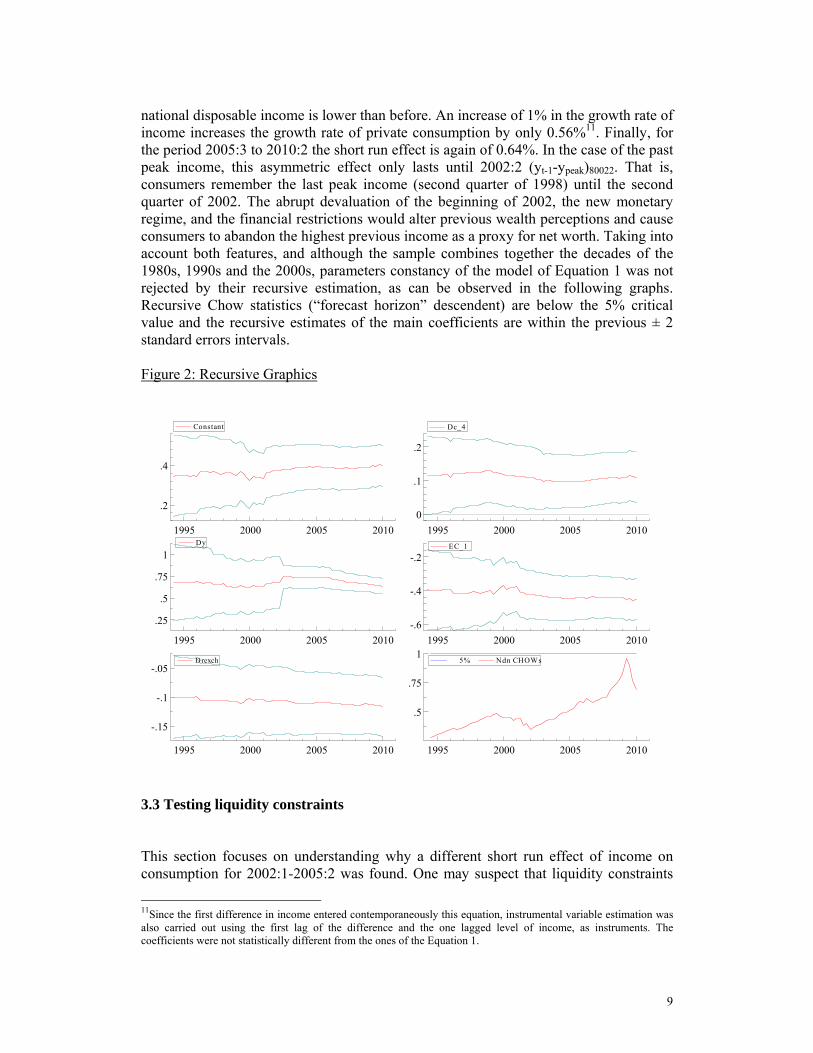
national disposable income is lower than before. An increase of 1% in the growth rate of income increases the growth rate of private consumption by only 0.56%11. Finally, for the period 2005:3 to 2010:2 the short run effect is again of 0.64%. In the case of the past peak income, this asymmetric effect only lasts until 2002:2 (yt-1-ypeak)80022. That is, consumers remember the last peak income (second quarter of 1998) until the second quarter of 2002. The abrupt devaluation of the beginning of 2002, the new monetary regime, and the financial restrictions would alter previous wealth perceptions and cause consumers to abandon the highest previous income as a proxy for net worth. Taking into account both features, and although the sample combines together the decades of the 1980s, 1990s and the 2000s, parameters constancy of the model of Equation 1 was not rejected by their recursive estimation, as can be observed in the following graphs. Recursive Chow statistics (“forecast horizon” descendent) are below the 5% critical value and the recursive estimates of the main coefficients are within the previous ± 2 standard errors intervals. Figure 2: Recursive Graphics

1995 2000 2005 2010

.2

.4

Constant

1995 2000 2005 20100

.1

.2

Dc_4

1995 2000 2005 2010

.25

.5

.75

1Dy

1995 2000 2005 2010-.6

-.4

-.2EC_1

1995 2000 2005 2010

-.15

-.1

-.05Drexch

1995 2000 2005 2010

.5

.75

1 5% Ndn CHOWs

3.3 Testing liquidity constraints This section focuses on understanding why a different short run effect of income on consumption for 2002:1-2005:2 was found. One may suspect that liquidity constraints

11Since the first difference in income entered contemporaneously this equation, instrumental variable estimation was also carried out using the first lag of the difference and the one lagged level of income, as instruments. The coefficients were not statistically different from the ones of the Equation 1.

10

are binding after the 2002 break because access to capital markets by Argentina was severely restricted, reverting the effect of the financial liberalization experienced during the 1990’s. Although financial flows to emerging countries had been decreasing since the Russian crisis (the “sudden stop” of Calvo, Izquierdo and Talvi, 2002), after the sovereign debt default, the Argentine economy faced further credit restrictions arising from both external and domestic sources. Not only did capital outflows accelerated but also, at the same time, there was also a domestic credit disruption because of financial restrictions and the asymmetric pesification of bank deposits and loans which took place after devaluation (Miller, et.al., 2004). Although the Argentine financial system tended to recover in the following months, credit to the private sector remained below the previous levels until year 2005. The credit expansion was driven by the strong growth that the economy experienced after the prolonged recession that it had suffered for several years.

As presented in section 3.1, an EC model can be used to test liquidity constraints by considering the shadow price of credit constraints depending on the EC terms. Under these restrictions, the estimated coefficient of Δyt and yt-1 should be equal (δ1 = δ2 in (1)). Therefore this hypothesis provides an empirical approach to evaluate a necessary condition to observe liquidity constraints.

The multiplicative dummy indicates different behaviour before 2002:1 and after

2005:2. Before 2002 and after 2005:2 liquidity constraints are not found to be binding. In the case of Equation 1, which includes an EC term, such an interpretation is untenable given that the hypothesis of an equal response of consumption to Δyt and to the EC term is strongly rejected by the following linear restrictions statistic for the period 1980:1 to 2001:4 and the period starting in 2005:3. Wald test for linear restrictions: βΔyt =-βEC_1 LinRes F( 1,102) = 7.553 [0.0071] **

However, when this restriction is evaluated for the period 2002:1 to 2005:2 the

corrected short run effect of Δyt021052 (because of the multiplicative dummy) equals the adjustment coefficient of the EC term. Wald test for linear restrictions: βΔyt+βΔyt021052 =-βEC-1 LinRes F( 1,102) = 2.5267 [0.1150]

These findings suggest that Argentine consumers have suffered liquidity

constraints since the first quarter of 2002 to the second quarter of 2005 as the EC term can be interpreted as the shadow price of credit restrictions.

Furthermore, another way to evaluate the effect of credit restrictions on consumption consists in verifying an asymmetric response of consumption to rising or falling income, as Altonji and Siow (1987) and DeJuan and Seater (1999) proposed. Altonji and Siow (1987) analyzed the rational expectations lifecycle model with capital market imperfection and found an asymmetric response of consumption to income increases and decreases. Since the rate of returns on assets is higher (lower) when expected income increases (decreases), the growth rate of consumption will be larger

11

(smaller). De Juan and Seater (1999) consider that symmetric effects of income are associated with “rule of thumb” behaviour (βΔytpos=βΔytneg), while under liquidity constraints, the consumers’ response to positive changes in income should be greater than the response to negative changes (βΔytpos > βΔytneg). Given that household panel data are employed in both papers, to test this hypothesis for aggregate consumption it is assumed that there are fewer constrained consumers than unconstrained ones when income is increasing and vice versa. Besides, actual income growth (Δyt) is used as a proxy for the expected income growth. The next equation shows the results allowing for different coefficients for positive (Δytpos) and negative (Δytneg) income growth. Equation 2 also shows the results for different coefficient of income increases (Δytpos021052) and decreases (Δytneg021052) distinguishing the effect for the 2002-2005 period.

Equation 2

Δct= 0.3876 +0.1185 Δct-4 +0.6020 Δytpos - 0.0544 Δytpos021052 [SE] [0.0563] [0.0391] [0.0556] [0.0425] 0.6837 Δytneg -0.2880 Δytneg021052 +0.1254 (yt-1 - ypeak)80022 [0.0671] [0.0543] [0.05246] -0.4400 EC_1 -0.1209 Δrexcht -0.0690 Seas8592 [0.0656] [0.0352] [0.0087] +0.0246 d844 +0.0331 d914 +0.0273 d921 [0.0042] [0.0033] [0.0074] -0.0199 d931 -0.03162 d952 +0.0131 d022 [0.0043] [0.00275] [0.0011] R2=0.959 F(15,100)=157.1[0.0000] σ=0.014

Estimates show that income increases and decreases have a similar effect on the

growth rate of consumption during the period 1980-2001 and 2005:3 to 2010:2.

Wald test for linear restrictions: βΔytpos=βΔytneg LinRes F( 1,100) = 0.92753 [0.3378]

Therefore, during the period 1980:1 to 2001:4 and 2005:3 to 2010:2, liquidity

constraints are found not to be binding12.

Instead results are different for the period 2002:1-2005:2. It is important to notice that, although the effect of income decreases was significant for this period, the effect of income increases was not significant at traditional levels. This implies that during the period 2002:1-2005:2 income increases had a differential effect on consumption growth compared to income decreases. The statistic for testing the hypothesis is Wald test for linear restrictions: βΔytpos+βΔytpos021052=βΔytneg+βΔytneg021052 LinRes F( 1,100) = 7.0614 [0.0092] **

12The existence of liquidity constraints is re-evaluated using both approaches for the eighties before the Convertibility regime (1980:1-1991:1). The results show that models with liquidity constraints cannot describe the consumers’ behaviour. Liquidity constraints also are not binding when these tests are performed for different subperiods of the eighties.

12

As this linear restriction is rejected, it may be concluded that there is evidence of the presence of liquidity constraints after default and devaluation and until the second quarter of 2005.

To sum up, during the period 1980:1 to 2001:4 and 2005:3 to 2010:2 liquidity

constraints are found not to be binding neither when tested by asymmetric effects nor when EC term is interpreted as a shadow price of restrictions. Liquidity constraints are binding after the default of the sovereign debt and the abandonment of the Convertibility regime took place, when consumers appear to suffer restrictions in obtaining the necessary financial resources to fulfil their optimal consumption plans. But liquidity constraints last until 2005:2 when consumption and income reached unprecedented levels following the strong growth that the economy experienced after the prolonged recession that it had suffered for several years.

Excluding the latter period, the relationship between consumption and income

implied by the econometric model estimates could suggest the following interpretation. The LC-PIH could be assumed from the proportionality between consumers’ expenditure and income derived as a long run solution. And as Carroll (2001) has noticed, “neither liquidity constraints nor myopia is necessary to generate the high average marginal propensity to consume that Friedman (1957) deemed consistent with his conception of the permanent income hypothesis”. In the short run, not only the EC term affects the consumers’ expenditure. The presence of the past peak income (yt-1-ypeak) until 2002 can also be part of an adjustment to “wealth” as Ando and Modigliani (1963, p.80) express, “… if we interpret the role of highest previous income as that of a proxy for net worth, then Duesenberry-Modigliani consumption function can be considered as providing a good empirical approximation to the consumption function…”. For the eighties, nineties and twenties Argentine "wealth perception" was also based on the behaviour of the real exchange rate as suggested by Heymann and Sanguinetti (1998).

From a historical perspective, it can be noticed that during the unstable 1980s consumers learned about the high costs of inflation and tried to avoid contracts of more than a few weeks. In this context, credit restrictions would not be unusual. However, liquidity constraints were found to be non-significant in the aggregate13. On the one hand, wealthier consumers may have been using their liquid assets to mitigate these restrictions and to avoid decreases in consumption. On the other hand, seignorage revenues could have been another source of soft budget constraints which could have been used to subsidize consumption because in this period the government collected a substantial inflation tax. The 1990s, in contrast, were characterized by price stabilization and increases in output and consumption. The political and economic reforms, the liquidity of banking system and the international willingness to finance the economy, led consumers to behave optimistically, entering into debt contracts. They did not seem to consider that the growth trend reached during the Convertibility regime was temporary and might have turned downward at some time. This behaviour explains the absence of liquidity constraints in the model until the end of Convertibility. Instead, the 2002 default and devaluation generated a reversion in international and domestic credit behaviour and a breakdown of contracts that is captured in the model as the existence of 13Dummy variables for different income effects during the eighties were proved but resulted as not significant.

13

liquidity constraints until the second quarter of 2005. As Galiani, Heymann and Tommasi (2002) said “...One of the big challenges that the Argentine economy (and its policymakers) will be facing is to gradually reconstitute a credit system in which “typical” macroeconomic contingencies (such as movements in the real exchange rate) do not cause the danger of a breakdown”. The results indicate that the credit system was gradually recovered since liquidity constraints were found not to be binding since the third quarter of 2005. In order to sum up the results we found it can be noticed that an EC with long run homogeneity implies

titt YKC =

where the average propensity to consume (Kit) can have several determinants (say, i=1,2) as in the case of the model estimated.14 Let Kit be decomposed as follows,

ttit KKKK 210 ..= where K0 = exp (constant). On the one hand, if Yt is seen as accrual from assets, then

. ttt W LY =

where Wt denotes the stock of aggregate assets. However if Wt is greatly immeasurable as in the Argentine case, the concept of “perceived wealth” should be introduced. In this case K1t would be a function (k1) of the variables reflecting wealth “perception” like those found as significant in the estimated model , the change in the real exchange rate and the difference between current and last peak income,

( ))y-(y rexch, peak1-t11 Δ= kK t Then, K1t Yt denotes the accrual from “perceived” wealth. On the other hand, if liquidity constraints are “regime dependent”,

( )t22 yΔ= tt IkK where, It=1= indicator of no liquidity constraints if Dt=0 It≠1= hj (Δyt) = liquidity constraints if Dt=1 When liquidity constraints hold (Dt=1), the hypothesis 14 It should be noticed that in the simpler EC model of Eq. (1) K only depends on the steady state growth rate of income and consumer expenditure.

14

H1 : βposΔyt = βnegΔyt should be rejected, and the hypothesis H2 : βΔyt =-βEC should not be rejected. Testing both hypotheses we found no evidence of liquidity constraints on Argentine consumers´ expenditure for the whole sample 1980-2010 except during 2002:1-2005:2 period when they help to explain the parameter change showed by the short run income effect. 4. Discussing co-breaking Co-breaking consists in the removal of deterministic shifts through the linear combination of the variables. Deterministic shifts can be found in the univariate representation of consumption and income: broadly the 1980´s, the 1990´s and the 2000´s. However, they are very similar for both series. Besides, assuming that the I(1) nature is maintained throughout the whole sample (as the unit root statistics reported indicated) cointegration results would imply co-breaking. Specifically, common trends and cointegration vectors are shown to be co-breaking vectors for equilibrium means and growth-rate shifts respectively (see Clements and Hendry, 1999 and Hendry and Massmann, 2007).

To further analyse cobreaking, following Hendry and Mizon (1998), we add step dummies for these periods to the system. Considering the standard case without breaks, the estimated eigenvalues seem to indicate (at traditional levels) a full rank long-run matrix that suggested stationary variables in the system (if this were not the case the long run coefficient still remains one). As the critical values are different from those of the standard case without breaks, we take into account the critical values for the rank statistics obtained from the response surfaces provided by Johansen, Mosconi and Nielsen (2000), even according to them, the same conclusions are maintained. For that reason we further evaluate cobreaking of consumption-income with co-breaking vector (1 -1) using the EC model obtained in the previous section. It is worth while noting that Equation 3 is parameterised in I(0) either if consumption and income are I(1) and cointegrated or both stationary around a segmented trend. However, these shifts could not remain in the conditional model in either case if they have a co-breaking relationship. Therefore, we added the step dummies to adjust the constant in the equilibrium correction formulation for these sub-samples. They were both individually and jointly not significant as the following results indicate,

15

Equation 3 Δct= 0.3810 + 0.1043 Δct-4 + 0.6402 Δyt - 0.07472 Δyt021052 [SE] [0.0641] [0.0389] [0.0427] [0.0298]

+0.1256 (yt-1 - ypeak)80022 - 0.4342 EC_1 - 0.1160 Δrexcht [0.0458] [0.0736] [0.0328] -0.0724 Seas8592 + 0.0241 d844 + 0.0347 d914 [0.0101] [0.0057] [0.0036] +0.0306 d921 - 0.0219 d931 - 0.0309 d952 [0.0084] [0.0042] [0.0032] +0.0140 d022 + 0.0020 d80911 - 0.0021 d021102 [0.0011] [0.0044] [0.0030] R2=0.959 F(15,100)=157.52[0.0000] σ=0.014 Wald test for linear restrictions: βd801911=0;βd021102=0 LinRes F( 2,100) = 0.60223 [0.5496]

These statistics show cobreaking for consumption and income as the breaking trends shown by the univariate representation of each series are cancelled out. Since the explained variable is expressed in growth rates these steps dummies would have represented different trend coefficients for levels and /or a different long run mean for different regimes. However, once the effects of liquidity constraints are taken into account such shifts are not significant.

5. Conclusions This paper has examined an empirical model of consumer behaviour for an economy subject to structural breaks and regime shifts. Following a general-to-specific approach we developed for Argentina (1980-2010) an Equilibrium-Correction (EC) model whose parameter estimates were used to test liquidity constraints vs. wealth effects. The concept of co-breaking has also been analysed.

The results have shown that even for an unstable economy like Argentina suitable models for consumer decisions can be developed once that parameter non-constancy is seen as informative about a different aggregate behaviour resulting from a regime change. That applies to the period after 2002 when a new monetary, exchange rate and financial regime dramatically changed the institutional background that had prevailed for over ten years. After the government defaulted and abandoned a Convertibility regime, evidence on liquidity constraints are found from an EC model but it lasts for 14 quarters until consumption reached the highest level since 1980. Although the deterministic components of consumption and income varied across the sub-samples, a long run relation of homogeneity lasts for the whole sample, confirming the co-breaking nature of the series. An EC model has allowed us to test liquidity constraints by considering the shadow price of credit constraints depending on the EC terms and taking into account asymmetric effects of rising and falling income. In both cases, liquidity constraints were rejected for the period 1980:1-2001:4 and 2005:3-2010:2. For these sample periods, the

16

estimated model was interpreted as one from the LC-PIH adapted to the Argentine experience by including two short run indicators of wealth perception: the deviations between current income and its last peak until 2002:2 and the growth rate of the real exchange rate for the whole sample. During the 2002:1-2005:2 period, instead, the same tests indicate that the hypothesis of liquidity constraints is not rejected, as consumers seem to feel the lack of the necessary financial resources to fulfil their optimal consumption plans.

17

Appendix 1: Data Definitions and Sources Private Consumption: Aggregate expenditure in goods and services of private residents and non-profit institutions. Economic Commission for Latin America (ECLAC), Buenos Aires and Dirección Nacional de Cuentas Nacionales (INDEC). Disposable Income: the gross national income plus the current net transfers. Economic Commission for Latin America (ECLAC), Buenos Aires and Dirección Nacional de Cuentas Nacionales (INDEC). Real Exchange Rate: Ratio of wholesale to consumer prices. Dirección Nacional de Cuentas Nacionales (INDEC). Real exchange rate peso/dollar. BCRA. Sovereign Risk: EMBI of Argentina. Carta Económica (Estudio Broda). Inflation: (pt –pt-1), where pt is the log of the general level of consumer prices. INDEC.

Appendix 2: Unit – Root

Period Private Consumption Disposable Income1980:1-2010:2 ADF(5)= -2.319a ADF(5)= -2.120a

1980:1-1991:1 ADF(5)= -2.232b ADF(5)= -2.405b

1991:2-2001:4 ADF(5)= -0.176 ADF(5)= -0.2261991:2-2010:2 ADF(5)= -1.392c ADF(5)= -1.108c

Deterministic components:a constant and trend b constant c trend

Series

18

Appendix 3: Cointegration analysis

Table 1

Consumption, disposable income, sovereign risk, real exchange rate and inflation system 1980(1) to 2010(2) (2 lags and d823,d88,d902,d014,d021,d032 and constant unrestricted) λi Ho:r=p Max λi 95% Tr 95% 0.306402 p == 0 | 43.54** 39.88** 33.5| 85.82** 78.61** 68.5 0.185982 p <= 1 | 24.49 22.43 27.1| 42.28 38.73 47.2 0.106903 p <= 2 | 13.45 12.32 21.0| 17.8 16.3 29.7 0.033032 p <= 3 | 3.997 3.661 14.1| 4.344 3.979 15.4 0.002907 p <= 4 |0.3465 0.3174 3.8| 0.3465 0.3174 3.8 Eigenvectors β' Δc 1.0000 -0.88482 -0.024974 -0.0018547 0.0041270 Δy -0.34917 1.0000 0.37788 -0.59267 2.2671 Δsrteq 0.85326 -0.54755 1.0000 0.94935 -0.43811 Δrexchrate 0.37205 0.61632 -0.27496 1.0000 -0.13734 Δinfla -5.2085 8.8270 0.46635 -0.80264 1.0000 Adjustment coefficients α Δc -0.62581 -0.0069850 -0.039118 -0.0022456 0.0023104 Δy 0.046408 -0.014630 -0.040494 -0.0048246 0.0026215 Δsrteq 0.15462 -0.013135 -0.14368 0.018207 -0.0021549 Δrexchrate -0.13556 -0.045433 0.0091518 -0.016495 -0.00088451 Δinfla -0.086992 -0.15639 0.10581 0.068513 -0.0015079 Test LR(r=1) Ho: α0=0; Chi^2(1) = 7.3907 [0.0066] ** Ho: α1=0; Chi^2(1) = 0.0381 [0.8452] Ho: α2=0; Chi^2(1) = 0.1097 [0.7404] Ho: α3=0; Chi^2(1) = 0.2394 [0.6246] Ho: α4=0; Chi^2(1) = 0.0074 [0.9310] Ho: β2=0; Chi^2(1) = 18.975 [0.0000] ** Ho: β3=0; Chi^2(1) = 1.4501 [0.2285] Ho: β4=0; Chi^2(1) = 0.0063 [0.9362] Ho: β5=0; Chi^2(1) = 0.0191 [0.8900] LR is the likelihood ratio statistics assuming rank =1

Table 2

Consumption and disposable income system 1980(1) a 2010(2) (2 lags and d021,d053, constant unrestricted and trend restricted) λi Ho:r=p Maxλi 95% Tr 95% 0.184 p==0 |24.51** 23.69** 19.0| 34.57** 33.42** 25.3 0.080 p<=1 |10.06 9.727 12.3| 10.06 9.727 12.3 α β’ Δc -0.45224 0.0066964 1.0000 -0.88563 Δy 0.02066 0.0078602 -0.9408 1.0000 Test LR (r=1) Ho: α1=0; Chi^2(1) = 6.8687 [0.0088] ** Ho: α2=0; Chi^2(1) = 0.0198 [0.8880] Ho: β2=-1; Chi^2(1) = 2.3773 [0.1231]

19

References

Ahumada, H. and Garegnani, M.L. (2007) Testing Hyperbolic Discounting in Consumer Decisions: Evidence for Argentina, Economics Letters, 95, 1, 146-150. Ahumada, H. y Garegnani, M.L. (2004) An Estimation of Deep Parameters describing Argentine Consumer Behaviour, Applied Economics Letters, vol. 11, 11, September , 719-723. Ahumada, H. and Garegnani, M.L. (2002) Wealth Effects in the Consumption Function of Argentina: 1980-2000, Anales de la XXXVII Reunión Anual de la Asociación Argentina de Economía Política, Tucumán, Argentina. Altonji, G. and Siow, A. (1987) Testing the Response of Consumption to Income Changes with (Noisy) Panel Data, The Quarterly Journal of Economics, 102, 2, 293-328. Ando A. and Modigliani F. (1963) The “life cycle” hypothesis of saving: aggregate implications and tests, American Economic Review, 53, 55-84. Banerjee, A., Lumsdaine, R. and Stock, J. (1992) Recursive and Sequential Tests of the Unit-Root and Trend-Break Hypotheses: Theory and International Evidence, Journal of Business & Economic Statistics, 10, 3, 271-287. Calvo, G., Izquierdo, A. and Talvi, E. (2002) Sudden Stops, the Real Exchange Rate and Fiscal Sustainability: Argentina’s Lessons, Mimeo, IADB. Campos, J. and Ericsson, N. (2000). Constructive Data Mining: Modeling Consumers´ Expenditure in Venezuela, Econometric Journal, 2, 226-240. Reprinted in Campos J., Ericsson, N. and Hendry, DF Eds. (2005). General- to-Specific Modelling, The International Library of Critical Writings in Econometrics, Elgar Publishing Ltd., UK. Carroll, C. (2001) A Theory of the Consumption Function, With and Without Liquidity Constraints (Expanded Version), NBER Working Paper Series, Working Paper Nº 8387. Clements M.P. and D.F. Hendry (1999) Forecasting Non-stationary Economic Time Series. Cambridge, Mass. MIT Press. Davidson, J.E.H., Hendry, D.F., Srba, F. and Yeo, J.S. (1978) Econometric modelling of the aggregate time series relationship between consumers' expenditure and income in the United Kingdom, Economic Journal, 88, (1978), 661-692. Reprinted in Hendry, D.F., Econometrics: Alchemy or Science? de Brouwer, G. J. (1996) Consumption and Liquidity Constraints in Australia and East Asia: Does Financial Integration Matter?”, Research Discussion Paper 9602, Economic Research Department, Reserve Bank of Australia. DeJuan, J. and Seater, J. (1999) The permanent income hypothesis: Evidence from the consumer expenditure survey”, Journal of Monetary Economics, 43, 351-376. Duesenberry, J.S. (1949) Income, Saving and the Theory of Consumer Behaviour”. Cambridge, Harvard University Press.

20

Doornik, J. A. (2009) Autometrics, Chapter 4 in J. L. Castle and N. Shephard (Eds.) The Methodology and Practice of Econometrics: A Festschrift in Honour of David F. Hendry, Oxford University Press, Oxford, 88-121.

Doornik, J. A., and Hendry D.F. (2009a) Empirical Econometric Modelling, PcGive 13, Vol.I, Oxmetrics 6, Timberlake Consultants Ltd, London.

Doornik, J. A., and Hendry D.F. (2009b) Modelling Dynamic Systems, PcGive 13, Vol.II, Oxmetrics 6, Timberlake Consultants Ltd, London. Favero, C. (2001) Applied Macroeconometrics. Oxford University Press, Oxford. Friedman, M. (1957) A Theory of the Consumption Function. Princeton, Princeton University Press. Galiani, S., Heymann, D. and Tommasi, M. (2002) Missed Expectations: The Argentine Convertibility, The William Davidson Institute, University of Michigan Business School, William Davidson Working Paper Nº 515. Garegnani, M.L. (2008) Enfoques alternativos para la modelación econométrica del consumo en Argentina, Editorial de la Universidad Nacional de La Plata. ISBN: 978-950-34-0455-3. Giovannini, A. (1985) Saving and the Real Interest Rate in LDCs, Journal of Development Economics, 18, 197-217. Hamilton, J.( 1994) Time Series Analysis. Princeton, Princeton University Press. Hendry, D.F. (1988) The Encompassing Implications of Feedback versus Feed-forward Mechanisms in Econometrics. Oxford Economic Papers, 40, 132-149. Hendry, D.F and Massmann, M. (2007) Co-breaking: Recent Advances and a Synopsis of the Literature, Journal of Business and Economic Statistics, 25, 33-51. Hendry, D.F. and Mizon G. (1998) Exogeneity, Causality and Co-breaking in Economic Policy Analysis of a Small Econometric Model of Money in the UK. Empirical Economics, 23, 267-294. Hendry, D.F. and Neale, A.J. (1991) A Monte Carlo study of the effects of structural breaks on tests for unit roots. In P.Hackl and A.H. Westlund (Eds.), Economic Structural Change, Analysis and Forecasting, pp. 95-119. Berlin: Springer-Verlag. Hendry, D.F. and von Ungern-Sternberg, T. (1981) Liquidity and Inflation Effects on Consumers’ Expenditure, in A. S. Deaton (ed.), Essays in the Theory and Measurement of Consumers’ Behaviour. Cambridge, Cambridge University Press. Reprinted in Hendry, D. F., Econometrics: Alchemy or Science? (1993). Heymann, D. and Sanguinetti, P. (1998) Quiebres de Tendencia, Expectativas y Fluctuaciones Económicas, Desarrollo Económico, Publicación trimestral del Instituto de Desarrollo Económico y Social, Vol. 38, abril-junio, Nº 149. Johansen, S. (1988) Statistical Analysis of Cointegration Vectors, Journal of Economic Dynamics and Control, Vol. 12, N º2-3, 231-254.

21

Johansen, S. and Juselius, K. (1990) Maximun Likelihood Estimation and Inference on Cointegration-With Application to the Demand for Money, Oxford Bulletin of Economics and Statistics, Vol. 52, Nº2, 169-210. Johansen, S., Mosconi, R. and Nielsen, B. (2000) Cointegration Analysis in the Presence of Structural Breaks in the Deterministic Trend, Econometrics Journal, vol.3, pp.216-24 Miller, M., Fronti, J. and Zhang, L. (2004) Default Devaluation and Depression: Argentina after 2001, mimeo. Muellbauer, J. and Lattimore, R. (1995) The consumption function: A theoretical and Empirical Overview, in Pesaran and Wickens (eds.), Handbook of Applied Econometrics: Macroeconomics. Blackwell Publishers, Oxford, 221-311. Muellbauer, J. and Bover, O. (1986) Liquidity Constraints and Aggregation in the Consumption Function under Uncertainty, Discussion Paper 12, Oxford, Institute of Economic and Statistic. Perron, P. (1989) The great crash, the oil price shocks and the unit root hypothesis. Econometrica, 57, 1361-1401 Rappoport P. and Reichlin L.(1989) Segmented trends and non-stationary time series. Economic Journal, 99, 168-177 Rossi, N. (1988) Government Spending, the Real Interest Rate and the Behavior of Liquidity-Constrained Consumers in Developing Countries, IMF Staff Papers, Vol. 35, 104-140.