modelling domestic water demand an agent based approach
DESCRIPTION
Modelling Domestic Water Demand an Agent Based ApproachTRANSCRIPT

lable at ScienceDirect
Environmental Modelling & Software 79 (2016) 35e54
Contents lists avai
Environmental Modelling & Software
journal homepage: www.elsevier .com/locate/envsoft
Modelling domestic water demand: An agent based approach
Ifigeneia Koutiva*, Christos MakropoulosDepartment of Water Resources and Environmental Engineering, School of Civil Engineering, National Technical University of Athens, Heroon Polytechneiou5, Athens GR 157 80, Greece
a r t i c l e i n f o
Article history:Received 28 May 2015Received in revised form26 September 2015Accepted 22 January 2016Available online xxx
Keywords:Agent based modellingDomestic water demand behaviourUrban water demand managementWater conservation
* Corresponding author.E-mail addresses: [email protected] (I. Ko
(C. Makropoulos).
http://dx.doi.org/10.1016/j.envsoft.2016.01.0051364-8152/© 2016 Elsevier Ltd. All rights reserved.
a b s t r a c t
The urban water system is a complex adaptive system consisting of technical, environmental and socialcomponents which interact with each other through time. As such, its investigation requires tools able tomodel the complete socio-technical system, complementing “infrastructure-centred” approaches. Thispaper presents a methodology for integrating two modelling tools, a social simulation model and anurban water management tool. An agent based model, the Urban Water Agents' Behaviour, is developedto simulate the domestic water users’ behaviour in response to water demand management measuresand is then coupled to the Urban Water Optioneering Tool to calculate the evolution of domestic waterdemand by simulating the use of water appliances. The proposed methodology is tested using, as a casestudy, a major period of drought in Athens, Greece. Results suggest that the coupling of the two modelsprovides new functionality for water demand management scenarios assessment by water regulatorsand companies.
© 2016 Elsevier Ltd. All rights reserved.
1. Introduction
The urban water system is a complex adaptive systemcomposed of technical, environmental and social components(water infrastructure, water resources and water users respec-tively) which interact dynamically and continuously with eachother and whose relationships evolve in time, particularly in viewof the dynamic and bottom up nature of water demand behavioursand patterns, thus increasing the uncertainty regarding itsresponse to changes and interventions (House-Peters and Chang,2011). More integrated, system-level approaches to the urbanwater cycle, attempting to manage both supply and demand,through an unified urban cycle management framework haverecently been emerging in the literature (including for exampleRozos and Makropoulos, 2013; Behzadian et al., 2014; Bach et al.,2014), but even these, leave the water end-user essentially out ofthe simulation domain.
Two of the main challenges in embedding the water end-userinto the urban water cycle are (a) the estimation of the behaviourof households in terms of water demand and (b) the quantificationof the way in which this behaviour is affected by water demand
utiva), [email protected]
management measures such as awareness raising campaigns andwater price changes.
In this paper, the water demand behaviour of urban householdsis simulated using theories from the social psychology domain, thatprovide a conceptual model of how human attitude is influencedand shaped by others (Allport, 1954; Hogg and Vaugnan, 2011) andof the potential association between attitudes, intentions andactual behaviours (Ajzen,1991). The proposedmethodology aims toexplore the change of water conservation attitude (from negative topositive). Such a change may be attributed to influence by, interalia, a small initial group of “water savers” whose own attitudediffers from the social norm (Fell et al., 2009). The main socialtheory that provides the computational tools to investigate thisinfluence while also taking into account social norms and externalinfluences is Social Impact Theory (Latane, 1981) and as such it wasselected for use within this framework.
The simulation environment, selected to setup and model theimplications of social psychology theories on the behaviour ofwater users is Agent Based Modelling (ABM). ABM has the ability tocapture emerging (bottom-up) behaviour, simulating the dynamicinteraction between the socio-economic and the water system andhence to provide the missing link to modelling the complete socio-technical water system as one (Wheater et al., 2007; Koutiva andMakropoulos, 2011; Barthelemy et al., 2001; Filatova et al., 2013).ABM uses intelligent agents defined as “computer systems situatedin some environment, capable of autonomous action in this
I. Koutiva, C. Makropoulos / Environmental Modelling & Software 79 (2016) 35e5436
environment in order to meet its design objectives” (Wooldridge,1999). Essentially, ABM is a form of computational social science(Gilbert, 2008) where agents are able to support emergence thuscreating complex behaviour from the interaction of simplecomponents.
ABM is slowly gaining ground in the water sciences field,starting with the coordination for water management in the Bali-nese water temple networks (Lansing and Kremer, 1994) and fol-lowed by several research efforts to create ABMs to simulate social-physical system interactions. Becu et al. (2003) used ABM forsimulating social dynamics for different control levels in a catch-ment in North Thailand, Athanasiadis et al. (2005) created an ABMfor simulating water consumers’ social behaviour and combined itwith an econometric model for evaluating water-pricing policieswhile Barthel et al. (2008) used an ABMmodel within the DANUBIADSS to simulate the behaviour of both the domestic water users andthe water supply sector in the Upper Danube Catchment in Ger-many. More recently, Galan et al. (2009a, b) created an ABM tosimulate domestic water demand in Valladolid, Spain. Anotherinteresting application of ABM to the water resources managementfield is the contribution of van Oel et al. (2010) that exploredfeedback mechanisms between water availability and water use ina semi-arid river basin.
In this paper we develop an ABM, hereafter termed the UrbanWater Agents Behavioural Model (UWAB), which simulates theurban household's water demand behaviour based on: (a) complexnetwork theory (Newman, 2003) representing the links among thedomestic water users of a city; (b) social impact theory (Latane,1981) addressing the effects of society, policies and other externalforces on the domestic users' behaviour; (c) the theory of plannedbehaviour (Ajzen, 1991) deconstructing the domestic water user'sbehaviour into components for modelling behavioural intention;and (d) statistical mechanics (Shell, 2014) employed to deal withthe inherently stochastic nature of human behaviour.
These theories have been partially exploited to analyse similarresearch problems in the past. For example, the theory of plannedbehaviour has been combined with social research methods toassess water demand behaviour (Hurlimann et al., 2009; Jorgensenet al., 2009; Fielding et al., 2010), while the same theory coupledwith ABM has been used to simulate individual domestic waterhabits (Schwarz and Ernst, 2009, Linkola et al., 2013). Social impacttheory has been used together with cellular automata (Latane,1996; Nowak and Lewenstein, 1996), agent based models (Holystet al., 2000; Kacperski and Holyst, 2000) and complex networktheory (Aleksiejuk et al., 2002; Sobkowizc, 2003a and 2003b) for avariety of social simulation purposes. Statistical mechanic havebeen used so far to analyse existing models (Castellano et al., 2009)while in this research we use them to develop more generalbehaviour rules of domestic water demand. The combination ofComplex Network Theory, Social Impact Theory, Theory of PlannedBehaviour and Statistical Mechanics within an agent basedmodelling framework (UWAB) is a key innovation in the workpresented in this paper.
Results on behavioural changes due to demand managementpolicies and environmental pressures are simulated within theUWAB model and are then translated into specific domestic waterdemands through micro-simulation of in-house water appliancesusing the Urban Water Optioneering Tool (UWOT) (Makropouloset al., 2008). This approach exploits the potential of alreadymature, proven simulationmodels for urbanwater modelling whileenhancing their remit by developing the functionality required todirectly take into account the social component of water demand.The proposed model and approach is also applicable for use withother urban water system models to investigate the impact ofbehavioural change of domestic water users to the water cycle e
allowing for example a much more thorough assessment of theurban water system's response to alternative water demand man-agement strategies. The methodology and models are demon-strated using the 1988e1994 drought in Athens, recreating theresponse of city's water demand to thewater demandmanagementefforts of that period.
2. Material and methods
2.1. The Urban Water Agent Behaviour (UWAB) model
2.1.1. PurposeThe Urban Water Agent Behaviour (UWAB) model was created,
using the NetLogo agent programming language (Wilensky, 1999),to simulate the effects of environmental pressures and water de-mand management policies on water demand behaviour ofhouseholds focusing specifically on water conservation. There is awide variety of available ABM toolkits, with NetLogo, Swarm andRepast being the three platforms that are most commonly used asidentified in an analysis of 53 different ABM platforms by Nikolaiand Madey (2009). In this research, NetLogo was selected for rea-sons related to (i) ease of use, (ii) available support documentation,(iii) the existence of an active support community and (iv) theavailability of a significant number of freely available models tolearn and get inspired from (Thielle and Grimm, 2010; Voinov andBousquet, 2010). Unlike other agent based models that deal withdomestic water demand (e.g. Athanasiadis et al., 2005 or Galanet al., 2009a, b) this model does not include a statistical or econo-metric model of consumption and focuses only on the household'swater demand behaviour. Water consumption is then estimatedusing a model specifically developed to simulate demand from theappliance level all the way to the water source (UWOT e presentedin the following section). In this section the variables, processes anddesign concepts of the UWAB model are presented using the ODDprotocol (Grimm et al., 2006) in the form of a roadmap, followingrecommendations by Polhill et al. (2008).
2.1.2. Design conceptsUsing the ODD terminology, UWAB's design concepts can be
defined as follows:
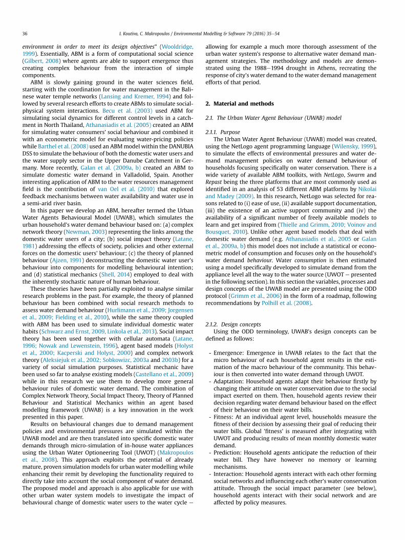
- Emergence: Emergence in UWAB relates to the fact that themicro behaviour of each household agent results in the esti-mation of the macro behaviour of the community. This behav-iour is then converted into water demand through UWOT.
- Adaptation: Household agents adapt their behaviour firstly bychanging their attitude on water conservation due to the socialimpact exerted on them. Then, household agents review theirdecision regarding water demand behaviour based on the effectof their behaviour on their water bills.
- Fitness: At an individual agent level, households measure thefitness of their decision by assessing their goal of reducing theirwater bills. Global 'fitness' is measured after integrating withUWOT and producing results of mean monthly domestic waterdemand.
- Prediction: Household agents anticipate the reduction of theirwater bill. They have however no memory or learningmechanisms.
- Interaction: Household agents interact with each other formingsocial networks and influencing each other's water conservationattitude. Through the social impact parameter (see below),household agents interact with their social network and areaffected by policy measures.

I. Koutiva, C. Makropoulos / Environmental Modelling & Software 79 (2016) 35e54 37
- Sensing: Household agents are assumed to know the waterconservation attitudes of their social network and to beinformed of the onset of a drought in their region.
- Stochasticity: UWAB introduces stochasticity in the selection ofthe water demand microstate that the household agent decidesto be in (see below).
2.1.3. State variables and scalesThe low level parameters of the household agents (Grimm et al.,
2006), their setup and descriptions are given in Appendix 1 cat-egorised per household agent's decision procedure whereappropriate.
2.1.4. Process overview and schedulingUWAB focuses on the urban population with each agent repre-
senting an urban household. The household agent population isdivided into three water user categories (low, average, high) thatrefer to an idealised “baseline” water demand profile of a givenhousehold. This profile is mainly linked to intrinsic motivation andself-determination in the behaviour of the household, whereintrinsically motivated and self-determined behaviours are taken tomean those that “represent the prototypes of self-determined orautonomous activities … that people do naturally and spontane-ously when they feel free to follow their inner interests.” (Deci andRyan, 2000). In other words, this baseline water demand profilerepresents a water use “intrinsic tendency” before the household isinfluenced by water demand management policies, its socialnetwork, or the weather. Although clearly this is an idealisedassumption, it is backed by a significant evidence base suggestingthat people's basic values are in their majority set by the time theyreach adulthood, and change relatively little thereafter (Rokeach,1968, Inglehart, 1971, 1977, 1997, 2008). This was further corrobo-rated by the qualitative socio-psychological research undertakenwithin this work (Gerakopoulou, 2013) where a panel of waterusers identified as the main driver their water demand behaviourto be their intrinsic motivation, created from internal individualvalues, such as environmental and economic values and life expe-riences. Panel members described their water use behaviours as aresult of experiences during childhood. For example “seeing theirgrand-parents bringing water from the village's central supply”made them aware of the value of water and the necessity to safe-guard it in everyday activities. Consequently, this water demand“category” follows a household agent throughout the simulation.Household agents of every category, however, are able to decidewhether or not to implement water conservation behaviour, butthe result of this behaviour differs from one category to another.
This decision making is realised by assuming that householdagents think about (and revise) at regular intervals (here everythree months, corresponding to the billing frequency in Athens)their attitude towards water conservation (positive or negative)and decide about their water demand behaviour, selecting one outof three (idealised) water conservation “levels” (zero, low or highconservation).
Household agents' attitudes towards water conservation areinfluenced by their social network and external factors, such aswater policies including water price changes and awareness raisingcampaigns. The interaction between different household agents,influencing their attitude and water demand behaviour, isapproached using network theory, as proposed by Sobkowizc(2009). To form the network, household agents are linked to eachother randomly using either NetLogo's “preferential attachment” or“small-world” code (Willenski, 2005a, b). It is acknowledged thatmore sophisticated approaches to complex network creation doexist (see for example Holme and Kim, 2002), but in this work we
opted to explore these two more elementary structures, in theabsence of alternative evidence for realistic network structures inour case study, for reasons of simplicity (they are both alreadyavailable in NetLogo). The network is expanded by using the sum ofthe difference of the socio-demographic characteristics of thepaired household agents as a proxy to the strength of the sociallinks thus allowing for the simulation of the effects of socialimmediacy (Sobkowizc, 2009).
Household agents with a negative attitude towards water con-servation can only select the “zero” water conservation level fortheir water demand behaviour state. On the other hand, householdagents with a positive attitude towards water conservation maychoose one out of all three water conservation levels (zero, low orhigh conservation). Household agents’ receive, every three months,water bills. The household agents compare their current water billwith their previous one and decide whether they prefer a higher,lower or the same level of conservation for their water demandbehaviour state. This preference is used by the household agents intheir water demand behaviour decision procedure.
The procedures followed by the household agents are shown inFig. 1 and explained in the following paragraphs.
2.1.5. SubmodelsUWAB utilises three key submodels: the social impact proce-
dure, the water demand behaviour procedure and the water de-mand behaviour review procedure.
Social impact procedure: During this procedure, the householdagent's water conservation attitude is affected by their own socialnetwork and external water policies. This effect (termed SocialImpact, I) is estimated using the Theory of Social Impact, intro-duced by Latane in 1981 and further developed by Nowak et al.(1990), supported by Bahr and Passerini's (1998) statistical me-chanics. Equation (1) calculates Social Impact (I) as a function ofpressure exerted by (a) each household agent's social network and(b) by water demand management policies currently in effect.
Ii ¼ �Sib� Oih�Xni;j ¼ 1
SjOjOi
d2i;j(1)
where,
Ii is the exerted social impact on household agent i who is amember of a social network of n other agents (j) (Ii E R).Oi (positive or negative) is the household agent's attitude onwater conservation (�1 or þ1)Si is the household agent's strength of influence (>¼0)b is the household agent's stubbornness (¼ 2)h is the external influence h ¼ SPCOPC þ SACΟAC where,SPC is the strength of influence regarding water price changesinformation (>¼0),OPC is the information regarding water price changes (if waterprices increase, then OPC is positive if prices decrease then OPC isnegative (�1 or þ1), creating a positive or negative influencetowards water conservation respectively)SAC is the strength of influence regarding awareness raisingcampaigns (>¼0) with a value of zero corresponding to anabsence of awareness raising campaignsOAC is the awareness campaign's attitude which is alwayspositive.
The term (Pn
i;j ¼ 1SjOjOi
d2i;j
) is the influence of the social network of
the household agent i that includes n other household agents j witheach member of the social network having a strength of influence
Fig. 1. Household agents' procedures.
I. Koutiva, C. Makropoulos / Environmental Modelling & Software 79 (2016) 35e5438
Sj, an attitude Oj and a social distance dij.Social distance (dij) measures the ease of communication be-
tween two individuals within a given population and is assumed to
be related to the proximity of an agent's socio-demographic char-acteristics to those of her peers based on Apolloni et al. (2009).
The result of the overall procedure is either a positive or a

I. Koutiva, C. Makropoulos / Environmental Modelling & Software 79 (2016) 35e54 39
negative attitude towards water conservation of household agent ifor the next three months of the simulation.
The magnitude of mutual interactions decreases with distance.The social distance is calculated by summing the differences of thesocial characteristics of the two linked household agents. If twolinked agents have the same socio-demographic characteristicsthey exert to each other the highest possible impact. They havehowever a social distance of 0 thus a value of one is added to thesocial distance equation as depicted in Equation (2):
dij ¼ 1þ������Xn
i;j;n¼1
xni � xnj
������ (2)
where,
dij is the social distance between the two linked householdagents i and j
Xni,j is the social characteristics of the two linked householdagents i and j with x equal to the household agent's variables for age(a), income level (i), education level (e), household occupancy (ho),housing type (renting or owning house) (ht).
Household agents run this procedure every three months andtheir attitude remains unchanged for the following three months.The probability that a particular agent i will change her attitude dueto social impact Ii is calculated using Equation (3). This is based onthe notion of “volatility” of social impact, introduced by Bahr andPasserini (1998), as a measure of an individual's susceptibility tochange, amended by Kacperski and Holyst (1999) to include a de-gree of randomness in the (otherwise deterministic) pressure.
Pchange ¼exp
�IiT
�
exp��Ii
T
�þ exp
�IiT
�
if X < Pchange 0Oiðtþ 1Þ ¼ �OiðtÞif X>Pchange0Oiðtþ 1Þ ¼ OiðtÞ
(3)
where,
Pchange is the probability of an individual changing their attitudeIi is the exerted social impactX is a randomly selected number from a uniform distribution of[0,1]Oi(t) is the attitude of the household agent i during the quarter t
T is the average volatility or social temperature of social impact(T � 0). Low values of T mean that household agents' attitudes arehighly dependent on their social network's attitudes, thus moreprobable to be affected by the social impact (Ii) exerted to them,whereas higher levels of T reduce the power of Ii in determining ahousehold agent's attitude. The parameter T is a measure of “socialtemperature” that captures the susceptibility to change of theaverage opinion within the simulated population (Kacperski andHolyst, 1999). Bahr and Paserini, in 1998, identified that socialtemperature is a group characteristic and not a personal charac-teristic, averaging a group's opinion susceptibility to change. Theygrounded this concept following the physical meaning of temper-ature which is a “global” characteristic that has no meaning inpairwise interactions (molecular) but is one of the main parametersin group interactions (gases). Analogue to this, “social temperature”is only valid in a statistical or average “large” group. The result ofthe overall procedure is either a positive or a negative attitude
towards water conservation of the household agent i for the nextthree months of the simulation.
Water demand behaviour procedure: It is understood that apositive attitude towards water conservation (such as the onederived from the social impact procedure above) does not neces-sarily lead to an actual water saving behaviour (Dolnicar andHurlimann, 2010). It only increases the chances of such a behav-iour actually taking place. Based on the Theory of Planned Behav-iour (TPB) (Ajzen, 1991) the attitudes and the subjective norms aresupplemented by the perceived behavioural control and alltogether act upon the behavioural intention to consume water in acertain manner. The stronger the intention the more likely is thebehaviour to be performed (Ajzen, 1991).
In the context of this work, a qualitative socio-psychologicalresearch was undertaken during 2013, working with a panel ofAthenian water users. The results of this study helped the identi-fication of the shaping factors of domestic water demand behav-iour. The most significant factors were identified as the effects ofawareness raising campaigns, one's intrinsic environmental con-sciousness, the end-user's socio-economic level and the expectedoutcome that water conservation could have on the water bill(Gerakopoulou, 2013). Based on these results as well as on anextensive literature review, a number of key factors affecting waterdemand behaviour were identified and are presented in Fig. 2 andexplained in the following paragraphs.
The factors presented abovewere used to create the behaviouralintention functions that household agents use for each one of thethree possible discrete states of water demand behaviour with low(BILC), high (BIHC) and zero (BINC) water conservation level(formulae are given in Appendix 1). As suggested above, everyhousehold agent estimates its behavioural intention every threemonths. The values of the behavioural intention's components havebeen selected in a way that the higher behaviour intention wouldcorrespond to a higher probability for water conservation (values ofthe parameters are given in Appendix 1).
The behavioural intention of each water demand behaviourstate is regarded as the “energy” of each state and every householdagent as a “thermodynamic system”, represented by a canonicalensemble of water demand behaviour states. Therefore, the prob-abilities of adopting each one of these states are estimatedfollowing Equation (4).
Plow conservation ¼ expðBILCÞ=ZPhigh conservation ¼ expðBIHCÞ=ZPno conservation ¼ expðBINCÞ=Z
(4)
where
Plow conservation is the probability of the household agent adopt-ing a state of water demand behaviour with low conservationlevelPhigh conservation is the probability of the household agentadopting a state of water demand behaviour with high conser-vation levelPno conservation is the probability of the household agent adoptinga state of water demand behaviour with zero conservation levelZ is the partition function that provides a normalization factorfor the probability distribution:Z ¼ exp(BILC) þ exp(BIHC) þ exp(BINC)
In order for the household agent to select one of the states ofwater demand behaviour a number between 0 and 1 is randomlyselected. The state whose probability is more than or equal to therandom number is then selected by the household agent.
Water demand behaviour review procedure: As suggested

Attitude- Environmental consciousness- Social Characteristics (age,
income, education, housing conditions)
- Past water saving attitude
Subjective norm- Social Network Impact
including the effects of water demand management measures
- Drought Conditions
Perceived Behavioural Control
- Ease or difficulty to decrease water demand based on household’s characteristics
- Effect of past water saving behaviour
BehaviouralIntention Behaviour
Fig. 2. Factors influencing actual water demand behaviour.
▪ Attitude relates to a favourable (or unfavourable) evaluation of the behaviour in question (Ajzen, 1991). Water users' conservation attitude relates to a number of socio-demographic factors such as: residents' age, income level, family size, education level and household characteristics (size, age, type of domestic water technologiesconfiguration) (Arbu�es et al., 2003; Barrett, 2004; Beal et al., 2011, Campbell et al., 2004; Fontdecaba et al., 2011; Harlan et al., 2009; Jones et al., 2011; Mondejar-Jimenezet al., 2011; Randolph and Troy, 2008; Willis et al., 2011). In addition, household's water conservation attitude is linked to water users' environmental attitude (Gilg andBarr, 2006), the weather (Baki et al., 2012; Koutiva et al., 2012) and past water saving behaviour (Gerakopoulou, 2013).
▪ Subjective norm towards the behaviour to conserve water is the perceived social pressure towards that behaviour (Ajzen, 1991). Perceived social pressure can beattributed to the impact of the social network and the effects of water demandmanagement measures such as awareness campaigns (Gregory and Di Leo, 2003) and waterprices changes (Jorgensen et al., 2009).
▪ Perceived behavioural control over the decision to conserve water is the ease or difficulty to perform a certain behaviour as perceived by the individual (Ajzen,1991). Thisis linked to the household agent‘s characteristics that affect its water demand behaviour and is represented in our model by a variable which is linked to the level of waterdemand of the household.
I. Koutiva, C. Makropoulos / Environmental Modelling & Software 79 (2016) 35e5440
earlier, each household agent is assumed to receive every threemonths a water bill. The water bills are calculated outside theUWABmodel, incorporating water pricing policies, and are insertedas external information to the model. The household agent com-pares the current water bill with the previous one and decideswhether it is more favourable to change its water demand behav-iour state or not. To this effect the model includes a variable in theestimation of the behavioural intention function of the water de-mand behaviour states with low and high water conservationlevels. Depending on the water demand behaviour state of thehousehold agent, the agent shows preference towards the same,lower or higher water conservation levels. For example, if an agentwith low water conservation receives a higher water bill than thatof the previous quarter then the household agent shows preferenceto the higher water conservation level (expecting a decrease to herwater bill in the next quarter). Additionally, if an agent receives thesame or higher water bill even though a conservation level isimplemented, she may decide to decrease her conservation level,thus increasing her consumption.
2.1.6. InitialisationThe UWAB is initialised by creating the population of household
agents and their social network. Household agents are assignedtheir descriptive characteristics (socio-demographics, householdtype, water user types etc) by sampling the distribution function ofthese attributes to the actual urban population. Finally, attitudestowards water conservation and water demand behaviour statesare randomly assigned to the household agent population.
2.1.7. InputUWAB requires the import of the different household agent
water user and household types and water demand behaviourstates.
At the end of each time step the UWAB model calculates thenumber of household agents that have selected each water demandbehaviour state.
2.2. Urban Water Optioneering Tool (UWOT)
UWOT is an urban water cycle model that utilises a bottom upapproach, simulating water demand generated by household ap-pliances, aggregating those at the household, neighbourhood andcity levels and then routing this demand all the way to the watersources (Rozos and Makropoulos, 2012). UWOT is used in this workto translate water demand behaviour (represented here by thefrequency of use of individual household appliances that use water,such as toilets, washing machines, and showers) into domesticwater demand.
UWOT's parameterisation requires identification of householdappliances and an estimation of their frequency of use for thedifferent water user types and water demand behaviour states(Rozos and Makropoulos, 2013; Beal et al., 2011, Grant, 2006). Theappliances' frequencies of use also account for annual and seasonaltrends. Seasonal variability is accounted for by changing the fre-quency of use of appliances that are affected by weather changessuch as the shower, the washing machine and outside uses (RozosandMakropoulos, 2013). The annual trend is incorporated across allin-house water appliances to capture the effects of a changingquality of life (under the assumption that as quality of life increasesso does overall frequency of use of water appliances).
Assigning frequency of uses for different conservation levels is achallenging task. To derive a reasonable estimate, different water
I. Koutiva, C. Makropoulos / Environmental Modelling & Software 79 (2016) 35e54 41
uses were divided into two separate categories: uses that coverbasic (non-discretional) everyday needs and uses covering discre-tional functions (Willis et al., 2011). Basic needs include drinkingwater, sanitation (flushing toilets), bathing (using the hand basin,shower, bath, washing machine) and kitchen activities (kitchensink and the dishwasher). Discretionary needs cover non-essentialwater uses, such as irrigation and outdoor activities. It is of courseunderstood that many basic water needs do include a largediscretionary component, such as showering or bathing for relaxingand not for sanitation purposes (Willis et al., 2011). Consequentlywhen exploring the water saving potential of a household, one mayalso include basic needs to those where water saving is feasible.
We then proceeded to identify the frequencies of use of appli-ances for both common and decreased water demand by under-taking a questionnaire-based research asking people how oftencertain appliances are being used in their households and howmuch they were willing to decrease this use in order to conservewater. The appliances’ frequencies of use time series were thenentered into UWOT.
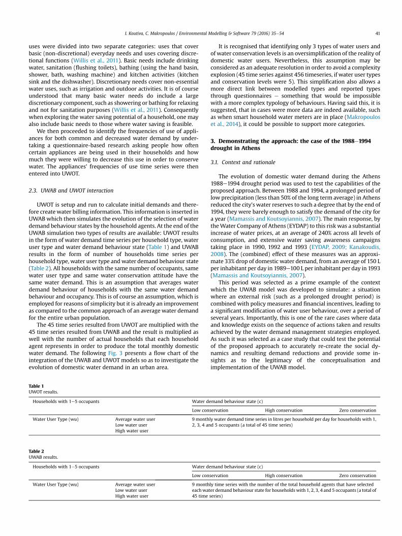
2.3. UWAB and UWOT interaction
UWOT is setup and run to calculate initial demands and there-fore createwater billing information. This information is inserted inUWAB which then simulates the evolution of the selection of waterdemand behaviour states by the household agents. At the end of theUWAB simulation two types of results are available: UWOT resultsin the form of water demand time series per household type, wateruser type and water demand behaviour state (Table 1) and UWABresults in the form of number of households time series perhousehold type, water user type andwater demand behaviour state(Table 2). All households with the same number of occupants, samewater user type and same water conservation attitude have thesame water demand. This is an assumption that averages waterdemand behaviour of households with the same water demandbehaviour and occupancy. This is of course an assumption, which isemployed for reasons of simplicity but it is already an improvementas compared to the common approach of an average water demandfor the entire urban population.
The 45 time series resulted from UWOT are multiplied with the45 time series resulted from UWAB and the result is multiplied aswell with the number of actual households that each householdagent represents in order to produce the total monthly domesticwater demand. The following Fig. 3 presents a flow chart of theintegration of the UWAB and UWOT models so as to investigate theevolution of domestic water demand in an urban area.
Table 1UWOT results.
Households with 1e5 occupants Water de
Low con
Water User Type (wu) Average water user 9 month2, 3, 4 anLow water user
High water user
Table 2UWAB results.
Households with 1e5 occupants Water de
Low con
Water User Type (wu) Average water user 9 montheachwat45 time
Low water userHigh water user
It is recognised that identifying only 3 types of water users andof water conservation levels is an oversimplification of the reality ofdomestic water users. Nevertheless, this assumption may beconsidered as an adequate resolution in order to avoid a complexityexplosion (45 time series against 456 timeseries, if water user typesand conservation levels were 5). This simplification also allows amore direct link between modelled types and reported typesthrough questionnaires e something that would be impossiblewith a more complex typology of behaviours. Having said this, it issuggested, that in cases were more data are indeed available, suchas when smart household water meters are in place (Makropouloset al., 2014), it could be possible to support more categories.
3. Demonstrating the approach: the case of the 1988e1994drought in Athens
3.1. Context and rationale
The evolution of domestic water demand during the Athens1988e1994 drought period was used to test the capabilities of theproposed approach. Between 1988 and 1994, a prolonged period oflow precipitation (less than 50% of the long term average) in Athensreduced the city's water reserves to such a degree that by the end of1994, they were barely enough to satisfy the demand of the city fora year (Mamassis and Koutsoyiannis, 2007). The main response, bytheWater Company of Athens (EYDAP) to this risk was a substantialincrease of water prices, at an average of 240% across all levels ofconsumption, and extensive water saving awareness campaignstaking place in 1990, 1992 and 1993 (EYDAP, 2009; Kanakoudis,2008). The (combined) effect of these measures was an approxi-mate 33% drop of domestic water demand, from an average of 150 Lper inhabitant per day in 1989e100 L per inhabitant per day in 1993(Mamassis and Koutsoyiannis, 2007).
This period was selected as a prime example of the contextwhich the UWAB model was developed to simulate: a situationwhere an external risk (such as a prolonged drought period) iscombined with policy measures and financial incentives, leading toa significant modification of water user behaviour, over a period ofseveral years. Importantly, this is one of the rare cases where dataand knowledge exists on the sequence of actions taken and resultsachieved by the water demand management strategies employed.As such it was selected as a case study that could test the potentialof the proposed approach to accurately re-create the social dy-namics and resulting demand reductions and provide some in-sights as to the legitimacy of the conceptualisation andimplementation of the UWAB model.
mand behaviour state (c)
servation High conservation Zero conservation
ly water demand time series in litres per household per day for households with 1,d 5 occupants (a total of 45 time series)
mand behaviour state (c)
servation High conservation Zero conservation
ly time series with the number of the total household agents that have selecteder demand behaviour state for households with 1, 2, 3, 4 and 5 occupants (a total ofseries)
1. ModellerEstimate in-house appliances’frequencies of use for all the
different water user types and water demand behaviour states
2. UWOTSimulate the evolution of the
domestic water demand for all the different water user types and
water demand behaviour states
3. ModellerCalculate the evolution of water
bills based on water pricing policies and UWOT results for all the different water user types andwater demand behaviour states
4. UWABSimulate the evolution of the
number of household agents’ that have selected the different water
demand behaviour states per water user type
5. ModellerCombine the results of UWOT and
UWAB to estimate total monthly water demand by multiplying the results of UWOT with the respective number of
household agents resulted from UWAB.
Fig. 3. Flow chart of the UWAB e UWOT interaction.
I. Koutiva, C. Makropoulos / Environmental Modelling & Software 79 (2016) 35e5442
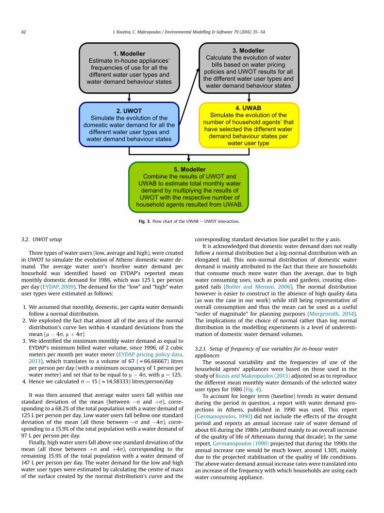
3.2. UWOT setup
Three types of water users (low, average and high), were createdin UWOT to simulate the evolution of Athens' domestic water de-mand. The average water user's baseline water demand perhousehold was identified based on EYDAP's reported meanmonthly domestic demand for 1986, which was 125 L per personper day (EYDAP, 2009). The demand for the “low” and “high”wateruser types were estimated as follows:
1. We assumed that monthly, domestic, per capita water demandsfollow a normal distribution.
2. We exploited the fact that almost all of the area of the normaldistribution's curve lies within 4 standard deviations from themean (m � 4s, m þ 4s)
3. We identified the minimum monthly water demand as equal toEYDAP's minimum billed water volume, since 1996, of 2 cubicmeters per month per water meter (EYDAP pricing policy data,2013), which translates to a volume of 67 (z66.66667) litresper person per day (with a minimum occupancy of 1 person perwater meter) and set that to be equal to m � 4s, with m ¼ 125.
4. Hence we calculated s ¼ 15 (z14.58333) litres/person/day
It was then assumed that average water users fall within onestandard deviation of the mean (between es and þs), corre-sponding to a 68.2% of the total populationwith a water demand of125 L per person per day. Low water users fall bellow one standarddeviation of the mean (all those between es and �4s), corre-sponding to a 15.9% of the total populationwith a water demand of97 L per person per day.
Finally, high water users fall above one standard deviation of themean (all those between þs and þ4s), corresponding to theremaining 15.9% of the total population with a water demand of147 L per person per day. The water demand for the low and highwater user types were estimated by calculating the centre of massof the surface created by the normal distribution's curve and the
corresponding standard deviation line parallel to the y axis.It is acknowledged that domestic water demand does not really
follow a normal distribution but a log-normal distribution with anelongated tail. This non-normal distribution of domestic waterdemand is mainly attributed to the fact that there are householdsthat consume much more water than the average, due to highwater consuming uses, such as pools and gardens, creating elon-gated tails (Butler and Memon, 2006). The normal distributionhowever is easier to construct in the absence of high quality data(as was the case in our work) while still being representative ofoverall consumption and thus the mean can be used as a useful“order of magnitude” for planning purposes (Morgenroth, 2014).The implications of the choice of normal rather than log normaldistribution in the modelling experiments is a level of underesti-mation of domestic water demand volumes.
3.2.1. Setup of frequency of use variables for in-house waterappliances
The seasonal variability and the frequencies of use of thehousehold agents’ appliances were based on those used in thestudy of Rozos andMakropoulos (2013) adjusted so as to reproducethe different mean monthly water demands of the selected wateruser types for 1986 (Fig. 4).
To account for longer term (baseline) trends in water demandduring the period in question, a report with water demand pro-jections in Athens, published in 1990 was used. This report(Germanopoulos, 1990) did not include the effects of the droughtperiod and reports an annual increase rate of water demand ofabout 6% during the 1980s (attributed mainly to an overall increaseof the quality of life of Athenians during that decade). In the samereport, Germanopoulos (1990) projected that during the 1990s theannual increase rate would be much lower, around 1.30%, mainlydue to the projected stabilisation of the quality of life conditions.The abovewater demand annual increase rates were translated intoan increase of the frequency with which households are using eachwater consuming appliance.

Fig. 4. UWOT results for 1986 monthly domestic water demand per month and mean monthly water demand from EYDAP datasets.
I. Koutiva, C. Makropoulos / Environmental Modelling & Software 79 (2016) 35e54 43
Finally, different time series of frequencies of use were createdfor all the different water user types and their correspondingwater conservation levels (averagewater user with low, high or noconservation level, low water user with low, high or no conser-vation level, high water user with low, high or no conservationlevel). The different conservation levels were created by using theresults of an online survey held in 2013. A set of questions wasincluded regarding the frequency of use of water appliances andthe willingness and % of frequency decrease that was acceptablefor different levels of water conservation. Since this socialresearch was conducted in 2013, one cannot of course suggest thatthe replies are fully representative of customs in 1986, but in theabsence of other data, these percentages of decrease for low andhigh conservation levels were utilised in setting up the appliances’frequencies of use for the different conservation levels (Fig. 5) inour simulation.
0%
10%
20%
30%
40%
50%
60%
70%
80%
90%
Kitchen sink Hand basin Dish washer T
In-house
esufoycneuqerffo
esaerced%
Low conservation (% decrease of frequency ofuse)High conservation (% decrease of frequency ofuse)
Fig. 5. % Change of the frequency of use for different ho
3.2.2. UWOT simulationFollowing the setup of the household appliances’ frequencies
of use for each water demand type and conservation level, UWOTwas set to run from 1986 to 1998 on a monthly basis (a total of156 timesteps). These results were used firstly to estimate thewater bills per household demand type and secondly to be in-tegrated with the UWAB results to estimate the total meanmonthly water demand of Athens population during the periodof 1986e1998.
3.3. UWAB implementation
The implementation of the designed modelling platform toAthens drought period requires the parameterisation of the modelso as to depict the social situation of Athens in the late 80s and early90s. The following paragraphs explain the parameterisation process
oilet Washingmachine
Shower Outdoor use
appliances
usehold appliances for different conservation levels.

Fig. 6. Example of UWAB's results, as time series of number of household agents that are average water users and perform no, low or high level of water conservation.
I. Koutiva, C. Makropoulos / Environmental Modelling & Software 79 (2016) 35e5444
as well as the sources used for setting up UWAB.
3.3.1. Setup of Athens household agentsIn 1981 Athens had about 850.000 households which increased
to about 1.000.000 households by 1991 (ELSTAT, 2012). Since it isimpractical in terms of simulation processing time to create about1.000.000 agents and simulate their behaviour, it was decided toaggregate the households with one household agent representing1000 households with the same preferences and characteristics(scaling down ratio ¼ 0.001).1 Consequently, in UWAB model, thesimulation begins with 930 household agents representing the930.000 households of Athens. Every twelve steps (i.e. every yearwith a time step being one month) 25 new household agents,representing 25.000 households, are created to demonstrate thepopulation increase that took place from 1986 to 1998.
The personal variables that need to be set during the UWABsetup are the socio-demographic and the social impact character-istics. These variables characterise the population and remainconstant throughout the simulation. Household agents are assignedlevels of socio-demographic characteristics consistent with socio-demographic characteristics distribution within the populationreported by the Office of National Statistics (ELSTAT, 2012). Theseinclude characteristics of education level, age and housing condi-tions. In addition, an income class categorization was used takinginto account both income and occupation (NCSR, 2006).
3.3.2. Water demand policies setupThe effect of the water price changes is usually evaluated using
an econometric approach (see Mylopoulos et al., 2004) which canbe combined with an ABM approach for evaluating water pricingpolicies (see Athanasiadis et al., 2005). UWAB tries to capture theeffect on the agents of the information that water price changes andnot the effect of the actual change in price. For that reason, pricing
1 Due to computing limitations it was necessary to scale down the population forthe simulation. Such scaling down is not uncommon in water use related agentbased models. For example, Galan et al. (2009a, b) created 12,500 agents forsimulating 125,000 families (scaling down ratio ¼ 0.1), Becu et al. (2003) created325 agents for simulating 2500 farmers (scaling down ratio ¼ 0.13), Athanasiadiset al. (2005), used 100 cellular automata for simulating more than a million ofdomestic water users (scaling down ratio ¼ 0.0001) and finally, Barthel et al. (2008)created 50000 agents for simulating a total of 10.8 millions of inhabitants of theupper Danube catchment (scaling down ratio ¼ 0.005).
policy is set as an external positive or negative force towards waterconservation affecting the social impact exerted to the householdagents. An increase or decrease of the water price is assumed toaffect the population by adding an external influence parameterpositive or negative towards water conservation.
From 1986 to 1998, water prices changed eight times, either as acorrection of thewater price levels (prior to 1990 and after 1993), oras a policy measure directly targeting the issue of the droughtduring the period 1988e1994 (EYDAP, 2009). The transmission ofthis information is assumed to start one month prior to the appli-cation of the water price change and to keep on affecting thehousehold agent for the next five months, leading to a total of a sixmonths “information effect period” for all price changes. EYDAPrecords suggest that water prices changed in the following months:01/07/1986, 01/07/1988, 0101/1990, 01/05/1990, 01/01/1991, 01/01/1992, 01/07/1992 and 01/12/1995.
The variables of water saving awareness campaigns that need tobe set are the influence strengths (SAC) and the implementationperiod.2 The influence strengths of the water saving awarenesscampaigns are experimental variables and were set during thecalibration process of the model. There were three implementationperiods of the campaigns: [01/01/1990e31/12/1990], [01/01/1992e31/12/1992] and [01/01/1993e31/12/1993] (EYDAP, 2009;Kanakoudis, 2008).
During 1993 authorities increased their efforts to reduce do-mestic water demand as much as possible. On top of the awarenesscampaigns and the water prices increase a series of water use re-strictions to outside uses and penalties to heavy water users werealso introduced (Kanakoudis, 2008). These extra water policiesdrastically affected Athenians, resulting in a 52% reduction of meanmonthly water demand, compared with the expected one(Kanakoudis, 2008). In this paper, these extra water policies areintroduced as two extra dummy parameters that are added to thebehavioural intention functions of the water conservation levelsduring the months of 1993. These dummy parameters increase the
2 The variability of the outcome was checked by performing 1000 repetitions ofone parameter set and checking the statistics of the outcome. Mean standarddeviation z 1 l/p/d (max st.dev. ¼ 2 l/p/d), Skewness ¼ �0.06 showing a slightlonger left tail of the values' probability distribution and Kurtosis ¼ 3.08 showing alarger peakedness than normal distribution. All the above, lead to the conclusionthat there is a very small variation of the model's outcomes and thus 10 repetitionsper parameter set up are acceptable.

Fig. 7. GLUE output uncertainty plot (automatically generated using the MCAT) (blue line ¼ observed values, grey area ¼ model output within confidence limits, dCFL ¼ normaliseddifference between upper and lower confidence limits). (For interpretation of the references to colour in this figure legend, the reader is referred to the web version of this article.)
I. Koutiva, C. Makropoulos / Environmental Modelling & Software 79 (2016) 35e54 45
probability for high and low water conservation level, thusincreasing the behavioural intention of the household and ulti-mately the probability to conserve water.
3.3.3. UWAB simulationFollowing the setup of the household agents, UWAB is ready to
simulate the behaviour of Athens’ household agents for 156months(termed “ticks” in NetLogo) from 1986 to 1998. UWAB results comein the form of number of household agents per water user categoryand conservation level (Fig. 6). The effect of both the awarenessraising campaigns and the water price changes is evident in Fig. 6.During 1990, 1992 and 1993 there is a significant behaviour changetowards water conservation for all three water user types.
3.4. Validation of the UWAB e UWOT modelling platform
The proposed modelling platform attempts to model the pat-terns and behaviours followed by urban households and have as aresult the evolution of domestic water demand under the influenceof water policy instruments. In order to do so, it is required to testwhether the model verifies the hypothesis that “under specifiedconditions, a macroscopic regularity of interest emerges” (Nikolicet al., 2012). In this specific case study, the output results aretested on their ability to recreate the evolution of the domesticwater demand from 1986 to 1998. The purpose of the proposedmodel is to catch the effects of the different water demand policiesto the household water demand behaviour thus exhibiting oscil-lations that match, to a certain extent, the observed ones.
3.4.1. Experimental variables’ sensitivity analysisThe modelling platform's results are estimated by combining
the results of the UWAB and UWOT models for the Athens casestudy. This is achieved bymultiplying the number of households foreach water user type and water conservation level with their cor-responding water demand. The eight experimental variables thatare used for the model's sensitivity analysis are (see Appendix 1(bold) for details):
- Mean strength of influence for household agents and externalinfluence (S)
- Mean strength of influence regarding awareness raising cam-paigns (SMAC)
- Mean strength of influence regarding water price changes(SMPC)
- Number of months before and after water price changes that theinformation is transmitted (M)
- Percentage of initial positive attitudes (ipa)- Percentage of external positive attitudes (epa)- Volatility of social impact (T)- Social network structure
As proposed by Nikolic et al. (2012), Latin hypercube samplingwas used to sample the multidimensional parameter space andcreate experiments for exploring the sensitivity of the proposedmodel parameters. One hundred parameter sets were selected andcorresponding experiments were created. These experiments wererepeated ten times each in order to decrease the influence of out-liers to the average result.2 The mean output of the ten repetitionsof each of the one hundred sampled parameter sets was used forthe sensitivity analysis of the proposed modelling platform.
As suggested, the main purpose of model validation in this caseis to show that the model follows the oscillations of the real worldobservations and that themodel is able to capture these oscillationswhilewater policies are in place. Consequently, one global objectivefunction was used, the Nash-Sutcliffe coefficient (Nash andSutcliffe, 1970), as it modified by Krause et al. (2005) and Herreraet al. (2010) (Equation (5)). The range of the modified Nash e
Sutcliffe coefficient lies between 0 (perfect fit) and þ∞. Values ofmore than one signify that the mean (median) value of the his-torical time series is a better predictor than the proposed model. Inaddition, a local objective function, the Mean Absolute PercentageError (MAPE) (Equation (6)), was used for measuring the diver-gence of the modelled results from the historical values during theintensive water policy response measures period of 1990e1993.
NS modified ðparskÞ ¼P156
i¼1�EWDi
�МWDiðparsiÞ= EWDi
�2P156
i¼1�EWDi
� EWDi= EWDi
�2(5)

Percentage of initial positive attitudes
.di | )deifid om
SN (.r tsi d .
mu c 0 0.1 0.2 0.3 0.4 0.5
0.2
0.4
0.6
0.8
1
Percentage of external positive influence
cum
. dis
tr.(N
Sm
odifi
ed) |
id.
0 0.2 0.4 0.6 0.8 1
0.2
0.4
0.6
0.8
1
Volatility of Social Impact
cum
. dis
tr.(N
Sm
odifi
ed) |
id.
20 40 60 80
0.2
0.4
0.6
0.8
1
mean Strength of Influence
.di | )deifi dom
SN(.r tsid .
muc 20 40 60 80 100
0.2
0.4
0.6
0.8
1
mean Media strength campaigns
cum
. dis
tr.(N
Sm
odifi
ed) |
id.
20 40 60 80
0.2
0.4
0.6
0.8
1
mean Media strength price
cum
. dis
tr.(N
Sm
odifi
ed) |
id.
20 40 60 80
0.2
0.4
0.6
0.8
1
Fig. 8. Identifiability plots for the model's parameters based on the modified Nash-Sutcliffe coefficient.
I. Koutiva, C. Makropoulos / Environmental Modelling & Software 79 (2016) 35e5446
MAPE ðparskÞ ¼
�����P12
i¼1�EWDi
� ðparsiÞ= EWDi
������total number of months
(6)
where, k denotes the parameter set under investigation (�0)
i denotes the result of the i-th month (1, 156)j denotes the monthly interval that calculates as well the totalnumber of months (e.g. j ¼ months 12e30, total number ofmonths ¼ 18)MWDi corresponds to the model's results for the i-th month,EWDi corresponds to the historical water demand for that i-thmonthEWDi
corresponds to the mean historical water demand for thati-th month and parsk corresponds to the respective k-th
Number of months before and after water price changes
Percentage of initial positive attitudes
.di|)E
PA
Mthguord(.rtsid.muc
0 0.1 0.2 0.3 0.4 0.5
0.2
0.4
0.6
0.8
1
Percentage of extecum
. dis
tr.(d
roug
htM
AP
E) |
id.
0 0.2 0.4
0.2
0.4
0.6
0.8
1
mean Strength of Influence
.di|)E
PA
Mth gu ord(. rts id.muc
20 40 60 80 100
0.2
0.4
0.6
0.8
1
mean Media stcum
. dis
tr.(d
roug
htM
AP
E) |
id.
20 40
0.2
0.4
0.6
0.8
1
.di|)E
PA
Mthgu ord(.r tsi d.m uc 1 2 3 4 5 6
0.2
0.4
0.6
0.8
1
Mean strength
Fig. 9. Identifiability plots for the model's parameter
parameter set, as selected from the Latin hypercube samplingprocess.
These objective functions and the Monte Carlo Analysis Toolbox(Wagener, 2004) were used for the model's experimental variablessensitivity analysis. Fig. 7 presents a Generalised Likelihood Un-certainty Estimation (GLUE) output plot for the modified Nash-Sutcliffe coefficient. This plot displays the model's output withassociated confidence intervals with 95% confidence level calcu-lated using the GLUE methodology. For each point in time a cu-mulative frequency distribution is generated using the selectedobjective (the modified Nash-Sutcliffe coefficient) and the confi-dence intervals calculated using linear interpolation. The bottomgraph is added to make the identification of regions with largeuncertainties easier to identify. It shows the difference betweenupper and lower confidence limit, normalised by the maximumdifference between the two over the investigated period of time
rnal positive influence0.6 0.8 1
Volatility of Social Impactcum
. dis
tr.(d
roug
htM
AP
E) |
id.
20 40 60 80
0.2
0.4
0.6
0.8
1
rength campaigns60 80
mean Media strength pricecum
. dis
tr.(d
roug
htM
AP
E) |
id.
20 40 60 80
0.2
0.4
0.6
0.8
1
campaigns Mean strength price changes
s based on the mean absolute percentage error.
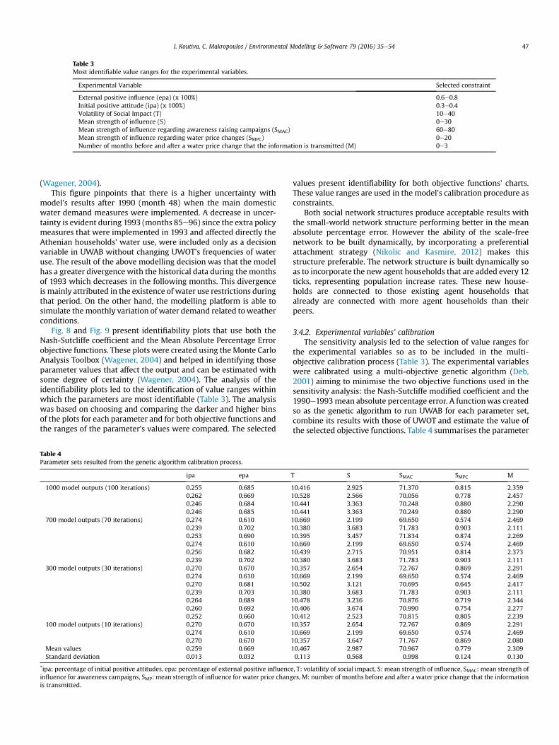
Table 3Most identifiable value ranges for the experimental variables.
Experimental Variable Selected constraint
External positive influence (epa) (x 100%) 0.6e0.8Initial positive attitude (ipa) (x 100%) 0.3e0.4Volatility of Social Impact (T) 10e40Mean strength of influence (S) 0e30Mean strength of influence regarding awareness raising campaigns (SMAC) 60e80Mean strength of influence regarding water price changes (SMPC) 0e20Number of months before and after a water price change that the information is transmitted (M) 0e3
I. Koutiva, C. Makropoulos / Environmental Modelling & Software 79 (2016) 35e54 47
(Wagener, 2004).This figure pinpoints that there is a higher uncertainty with
model's results after 1990 (month 48) when the main domesticwater demand measures were implemented. A decrease in uncer-tainty is evident during 1993 (months 85e96) since the extra policymeasures that were implemented in 1993 and affected directly theAthenian households' water use, were included only as a decisionvariable in UWAB without changing UWOT's frequencies of wateruse. The result of the above modelling decision was that the modelhas a greater divergence with the historical data during the monthsof 1993 which decreases in the following months. This divergenceis mainly attributed in the existence of water use restrictions duringthat period. On the other hand, the modelling platform is able tosimulate themonthly variation of water demand related toweatherconditions.
Fig. 8 and Fig. 9 present identifiability plots that use both theNash-Sutcliffe coefficient and the Mean Absolute Percentage Errorobjective functions. These plots were created using theMonte CarloAnalysis Toolbox (Wagener, 2004) and helped in identifying thoseparameter values that affect the output and can be estimated withsome degree of certainty (Wagener, 2004). The analysis of theidentifiability plots led to the identification of value ranges withinwhich the parameters are most identifiable (Table 3). The analysiswas based on choosing and comparing the darker and higher binsof the plots for each parameter and for both objective functions andthe ranges of the parameter's values were compared. The selected
Table 4Parameter sets resulted from the genetic algorithm calibration process.
ipa epa
1000 model outputs (100 iterations) 0.255 0.6850.262 0.6690.246 0.6840.246 0.685
700 model outputs (70 iterations) 0.274 0.6100.239 0.7020.253 0.6900.274 0.6100.256 0.6820.239 0.702
300 model outputs (30 iterations) 0.270 0.6700.274 0.6100.270 0.6810.239 0.7030.264 0.6890.260 0.6920.252 0.660
100 model outputs (10 iterations) 0.270 0.6700.274 0.6100.270 0.670
Mean values 0.259 0.669Standard deviation 0.013 0.032
*ipa: percentage of initial positive attitudes, epa: percentage of external positive influenceinfluence for awareness campaigns, SMP: mean strength of influence for water price changis transmitted.
values present identifiability for both objective functions' charts.These value ranges are used in the model's calibration procedure asconstraints.
Both social network structures produce acceptable results withthe small-world network structure performing better in the meanabsolute percentage error. However the ability of the scale-freenetwork to be built dynamically, by incorporating a preferentialattachment strategy (Nikolic and Kasmire, 2012) makes thisstructure preferable. The network structure is built dynamically soas to incorporate the new agent households that are added every 12ticks, representing population increase rates. These new house-holds are connected to those existing agent households thatalready are connected with more agent households than theirpeers.
3.4.2. Experimental variables’ calibrationThe sensitivity analysis led to the selection of value ranges for
the experimental variables so as to be included in the multi-objective calibration process (Table 3). The experimental variableswere calibrated using a multi-objective genetic algorithm (Deb,2001) aiming to minimise the two objective functions used in thesensitivity analysis: the Nash-Sutcliffe modified coefficient and the1990e1993mean absolute percentage error. A functionwas createdso as the genetic algorithm to run UWAB for each parameter set,combine its results with those of UWOT and estimate the value ofthe selected objective functions. Table 4 summarises the parameter
T S SMAC SMPC M
10.416 2.925 71.370 0.815 2.35910.528 2.566 70.056 0.778 2.45710.441 3.363 70.248 0.880 2.29010.441 3.363 70.249 0.880 2.29010.669 2.199 69.650 0.574 2.46910.380 3.683 71.783 0.903 2.11110.395 3.457 71.834 0.874 2.26910.669 2.199 69.650 0.574 2.46910.439 2.715 70.951 0.814 2.37310.380 3.683 71.783 0.903 2.11110.357 2.654 72.767 0.869 2.29110.669 2.199 69.650 0.574 2.46910.502 3.121 70.695 0.645 2.41710.380 3.683 71.783 0.903 2.11110.478 3.236 70.876 0.719 2.34410.406 3.674 70.990 0.754 2.27710.412 2.523 70.815 0.805 2.23910.357 2.654 72.767 0.869 2.29110.669 2.199 69.650 0.574 2.46910.357 3.647 71.767 0.869 2.08010.467 2.987 70.967 0.779 2.3090.113 0.568 0.998 0.124 0.130
, T: volatility of social impact, S: mean strength of influence, SMAC: mean strength ofes, M: number of months before and after a water price change that the information

Fig. 10. Pareto fronts resulted from the multi-objective algorithmminimising both selected objective functions. Objective functions' results are given for different iteration numbers.
I. Koutiva, C. Makropoulos / Environmental Modelling & Software 79 (2016) 35e5448
sets that resulted from the multi-objective genetic algorithm runfor 10, 30, 70 and 100 iterations. Each iteration includes tendifferent parameter sets and therefore UWAB run for 100, 300, 700and 1000 times respectively. Fig. 10 presents the resulted Paretofronts.
The modelling platform was initialised based on the results ofthe optimisation process (Table 4, experimental variables values for1000 model runs given in the first four lines) and run 10 times foreach optimisation solution. Fig. 11 presents the results from theapplication of the UWOT-UWAB modelling platform to the Athens1988e1994 drought period. The mean modified Nash-Sutcliff co-efficient is 0.64 showing that the createdmodel is a better predictorthan the mean of the observed data and the mean MAPE (MeanAbsolute Percentage Error) for 1990e1993 period is 0.14, whichmeans a 14% absolute error within the estimated water demand forthe years were demand management policies were in place.
Fig. 11. Results of simulated Athens 1988e1994 drought period (blue line: EYDAP historical vreferred to the web version of this article.)
4. Discussion
Based on the taxonomy of ABMs created by Boero and Scquazoni(2005) the designed UWAB model is possible to be categorised as a“typification” model that analyses an empirical phenomenon syn-thesized of “a great many diffuse, discrete, more or less present andoccasionally absent concrete individual phenomena, which are ar-ranged according to those one-sidedly emphasized viewpoints intoa unified analytical construct” (Weber, 1904). The focus of thisresearch is the domestic water demand behaviour of urbanhouseholds and UWAB implements pieces of theories such as thesocial impact theory (Latane, 1981), the social network theory(Albert et al., 1999) and statistical mechanics (Shell, 2014) in orderto create the micro decision making process of household agents.The main aim of the model may be described as trying to “find amicro-macro generative mechanism that can allow explaining thespecificity of the case, and … to build upon it realistic scenarios for
alues). (For interpretation of the references to colour in this figure legend, the reader is

Fig. 12. Mean absolute percentage error per year.
I. Koutiva, C. Makropoulos / Environmental Modelling & Software 79 (2016) 35e54 49
policy making” (Boero and Scquazoni, 2005). The combination ofUWAB with UWOT allows the estimation of the “macro” meandomestic water demand from the “micro” domestic water demandbehaviour of urban households.
The implementation of UWAB to Athens' 1988e1994 droughtperiod is a “case-based model of empirically circumscribed phe-nomena, with specificity and “individuality” in terms of time-spacedimensions” (Boero and Scquazoni, 2005). This case was used inorder to validate the UWAB model's design features. The producedgoodness of fit is able to validate the UWAB model. In addition, themodel's output has identified several findings regarding the sys-tem's behaviour during the Athens drought period:
1. The 1993 reduction of water demand can bemainly attributed inthe water use restrictions. While the mean absolute percentageerror for 1990e1992 is around 10%, the mean absolute per-centage error for 1993 more than doubles at about 25% (Fig. 12).This difference in error is attributed in the water use restrictionsthat were imposed in 1993. This effect could be decreased if the1993 restrictions were included in the UWOTmodel. However, itwas decided not to integrate the restrictions in the UWOTmodelin order to have an indication of the effect of restrictions to theevolution of water demand.
Fig. 13. Mean monthly domestic water demand (purple line: EYDAP S.A. real values, all othcolour in this figure legend, the reader is referred to the web version of this article.)
2. The application of the modelling platform to the Athens droughtperiod presented a mean error of 10% (excluding the restrictionsmisleading effect). As seen in Fig. 4 the main differences werethe peaks of water demand. These inconsistencies may attrib-uted to the method of including the seasonal variation of waterdemand, altering the frequency of use for three appliancesbased on the study of Rozos and Makropoulos (2013). It may beassumed that an end of use study could give more insightregarding the seasonal use of water appliances. Yet, themodelling platform's results were able to capture the direction(decrease and increase) of domestic water demand. Fig. 13presents the mean monthly water demand resulted from theUWOT-UWAB modelling platform (Table 4, experimental vari-ables values for 1000 model runs given in the first four lines) incomparison with the mean monthly demand as taken fromEYDAP S.A. report (EYDAP, 2009).
3. The historical data are best fitted with a much lower strength ofinfluence for water price changes than the strength of influencefor awareness campaigns. In this work only the informationregarding water price changes was incorporated in the decisionrules of the household agents. It is assumed, for the case study ofthe Athens drought period that all eight water price changesthat occurred during the simulation period have the samestrength of influence to Athens population. Nonetheless, what is
er colours: modelled results of water demand). (For interpretation of the references to

I. Koutiva, C. Makropoulos / Environmental Modelling & Software 79 (2016) 35e5450
actually affecting the behaviour is not just the information butalso the amount of change. A further step of this model would beto incorporate an econometric rule that would simulate the ef-fect of the actual water price change in the water demandbehaviour.
4. This research approaches water price changes in a novelmanner, drawing conclusions from both theory and the selectedcase study and applying them in the proposed methodology. Inparticular, the agents' water conservation attitude is affected bythe transmitted information regarding price changes and thewater demand behaviour from the effects of past saving be-haviours to the household's water bill. This is a new approach,focusing on the information about water price changes and notthe actual change, contrary to either the use of econometricfunctions for translating water price changes to water demand(Athanasiadis et al., 2005) or the exclusion of water priceschanges from behavioural rules (Galan et al., 2009a, b) under theassumption that water price is inelastic (Arbues et al., 2003).
5. The historical data are best fitted with low values of volatility ofsocial impact (T z 10). This result indicates that the societyunder investigation is rather susceptible to social norms effects.
A clear limitation of the work reported here is the need to makeseveral assumptions in the absence of extensive high quality dataabout water users and their behaviours. This is a challenge for allresearch in the field of computational social science and in ourwork this limitation has beenmanaged through sensitivity analysis,uncertainty analysis and calibration approaches. In so doing wehave also highlighted the types of crucial datasets that need to becollected in new case studies. A next step in this research would beto use the UWABmodel for another case study that would allow theparameterisation of the model with more data and fewer as-sumptions. It is evident that since there has not been yet animplementation of the developed model to a specific case that is“perfectly” understood and where all necessary data are available,the designed model might have several errors and artefacts (Galanet al., 2009a, b). Nevertheless, the model's results show that thehousehold agent population reacts in a “common sense” way,meaning it reconsiders its water conservation behaviour whensignals are sent regarding water prices changes and awarenesscampaigns and forgets about water saving, returning to its commonuse, when policies are not in place. This “looking right” model re-sults might indicate a sign of model verification (Crooks et al.,2008).
5. Conclusions
This paper illustrates the design concept of the Urban Water
Social characteristics
Variable Setup of parameter
income 2 {�1, 0, 1, 2} Require data from statistical offices for the distributioincome levels within the population.
age 2 {�1, 0, 1} Require data from statistical offices for the distributiolevels within the population.
edu-level 2 {�1, 0, 1} Require data from statistical offices for the distributioeducation levels within the population.
family-size 2 {1, 2, 3, 4, 5} Require data from statistical offices for the distributionsizes within the population.
housing 2 {0, 1} Require data from statistical offices for the distributiohousing types within the population.
envaware 2 {�2, �1, 0, 1, 2} Require data from statistical offices for the distributioenvironmental consciousness levels within the popula
Agents' Behaviour model that simulates the water demandbehaviour of urban households. The social environment, withinwhich the agents operate, is likened as a scale-free network. Theinfluence exerted to the water demand behaviour of the house-holds is simulated following social impact theory. In addition, therules of water demand behaviour include the shaping factors ofdomestic water demand e.g. socio-economic characteristics, relatedto the urban area under investigation. The final behaviour of theagents is decided using statistical mechanics (Shell, 2014) toincorporate stochasticity in the simulation of the agents' final de-cision. The model is implemented in the NetLogo programmingenvironment. The translation of the household's behaviour towaterdemand volumes is done using the Urban Water Optioneering Tool(UWOT). Finally, the integration of UWAB and UWOT is applied tothe Athens 1988e1994 drought and evaluated regarding its abilityto simulate the influence of water demand management measuresto the water demand behaviour of the Athenian households. Thisapplication allows the evaluation of the developed methodologyincluding the rules followed by the agents to simulate the house-holds' water demand behaviour.
The integration of UWAB with UWOT creates a modellingmethodology and platform that is able to assist an “experimental”management approach, such as the one proposed by adaptivewater resources management. Such water resources managementexperiments may allow the investigation of behavioural patterns,linkages and feedback loops to the management and performanceof the urban water system. The developed methodology allowsrunning several experiments for different scenarios so as to eval-uate the effect of water demand policies. Such an approach, givesthe opportunity to better understand the way the systemmay reactto changes and supports incremental adjustments on the man-agement decisions based on learning outcomes.
Acknowledgements
This research has been co-financed by the European Union(European Social Funde ESF) and Greek national funds through theOperational Program “Education and Lifelong Learning” of theNational Strategic Reference Framework (NSRF) - Research FundingProgram: Heracleitus II. Investing in knowledge society through theEuropean Social Fund.
Appendix 1. UWAB state variables
Experimental variables that were used for the sensitivityanalysis and the calibration of the modelling platform are givenin bold.
Brief description
n of Income level of the household agent (�1 ¼ low level, 0 ¼ low e middle,1 ¼ middle e high, 2 ¼ high)
n of age Age level of the household agent (�1 ¼ 19e34, 0 ¼ 35e64, 1 ¼ ¼> 65)
n of Education level of the household agent (�1 ¼ low, 0 ¼middle, 1 ¼ high)
of family Number of household members of the household agent
n of Housing type of the household agent (0 ¼ renters, 1 ¼ owners)
n oftion.
Environmental consciousness level of the household agent (�2 ¼ verylow environmental consciousness, �1 ¼ low environmentalconsciousness, 0 ¼ middle environmental consciousness, 1 ¼ highenvironmental consciousness, 2 ¼ very high environmentalconsciousness)

Water demand management policies
Variables Setup of parameter Brief description
water_bill_awater_bill_b
Requires information from UWOT Household agents receive every three months a water bill basedspecific to their water user type, water conservation level and the sizeof their household. The comparison between water bills allows thehousehold agents to review their decision regarding the waterconservation level.
price_change_info (�1, 0, 1) If a historical event is under investigation this is set based on thehistorical information available. If scenarios of domestic waterdemand evolution are explored this is set to explore different waterpricing policies.
The information onwater price change (�1¼ decrease of water price,0 ¼ stable water price, 1 ¼ increase of water price) creates an extrapositive or negative influence towards water conservation.
mean _strength_influence_price (SPC)
(>¼0)sd _strength_influence_price (0.8* SPC)
Experimental variable.If a historical event is under investigation this is a calibrationparameter. If scenarios of domestic water demand evolution areexplored this is set to explore different distributions of theinfluence strength regarding water price changes.
Mean and standard deviation of the distribution of the influencestrength within the urban population regarding water pricechanges.
onset_pricingend_pricing
If a historical event is under investigation this is set based on thehistorical information available. If scenarios of domestic waterdemand evolution are explored this is set to explore different waterpricing policies.
Number of ticks (months) since the beginning of the simulation that apricing policy begins and ends.
months_price_information(M)
Experimental variable.If a historical event is under investigation this is set based on thehistorical information available. If the information is notavailable this is a calibration variable. If scenarios of domesticwater demand evolution are explored this is set to exploredifferent water pricing policies.
Months (number of ticks) before and after a water price changeevent that the information is still transmitted.
onset_campaignend_campaign
If a historical event is under investigation this is set based on thehistorical information available. If scenarios of domestic waterdemand evolution are explored this is set to explore differentawareness raising campaigns policies.
Number of ticks (months) since the beginning of the simulation thatan awareness raising campaign begins and ends.
mean_strength_influence_awareness_campaigns (SAC) (>¼0)sd_strength_influence_ awareness_campaigns (0.8* SAC)
Experimental variable.If a historical event is under investigation this is a calibrationparameter. If scenarios of domestic water demand evolution areexplored this is set to explore different distributions of theinfluence strength regarding awareness raising campaigns.
Mean and standard deviation of the distribution of the influencestrength within the urban population regarding awarenessraising campaigns.
Awareness_Campaign (0, 1) Awareness raising campaigns regarding water conservation (0 ¼ nocampaign, 1 ¼ campaign) creates an extra positive or negativeinfluence towards water conservation.
Social impact procedure
Variables Setup of parameter Brief description
%þ_water_conservation (ipa) Experimental variable.Household agents are randomly assigned positive or negativeinitial positive attitude towards water conservation.
Initial percentage of population with positive attitude towardswater conservation.
opinion-watercons 2 {�1, 1} Household agent's decision parameter Water conservation attitude (�1 ¼ negative towards waterconservation, 1 ¼ positive towards water conservation)
influence_strength (>¼0) (S) Experimental variable Personal strength of influence sets the level of persuasivenessthat a household agent has towards “selling” its attituderegarding water conservation to its social network
opinion_strength (>¼0) Requires knowledge regarding the society's stubbornness. Set toa constant of 2 based on theory (Kacperski and Holyst, 1999; Bahrand Paserini, 1998; Wragg, 2006).
Personal attitude strength sets the level of stubbornness,measuring the difficulty to change its attitude regarding waterconservation.
%þ_ext_water_cons (epa) Experimental variable.Household agents are randomly assigned positive or negativeexternal influence.
Percentage of population with positive external influencetowards water conservation. Constant throughout thesimulation.
external_influence 2 {-1, 1} Household agents are randomly assigned positive or negativeexternal influence.
External connections' attitude (�1 ¼ negative towards waterconservation, 1 ¼ positive towards water conservation)
strength-external (>¼0) (S) Experimental variable.Household agents are randomly assigned a strength ofexternal influence sampled from a normal distribution wheremean and standard deviation are the experimental variables.
External connections' strength of influence sets the level ofpersuasiveness that the external social connections of thehousehold agent have towards “selling” their attituderegarding water conservation
Volatility_SocialImpact (>¼0) (T) Experimental variable.Constant for all household agents and throughout thesimulation.
T is the average volatility of social impact. The parameter T is ameasure of “social temperature” that captures thesusceptibility to change of the average attitude within thesimulated population (Kacperski and Holyst, 1999, Bahr andPaserini, 1998). High values of Tmean that attitudes are difficultto change and low values that attitudes are highly dependent onsocial norms (Wragg, 2006).
I. Koutiva, C. Makropoulos / Environmental Modelling & Software 79 (2016) 35e54 51

Water demand behaviour procedure
Variables Setup of parameter Brief description
low-user? (true/false)high-user? (true/false)mean-user? (true/false)
Requires information regarding the distribution of the water usertypes within the population.
Each household agent has a type of water user assigned from thebeginning of the simulation.
watercommonuse 2 {�1, 1}waterconslowlevel 2 {-1, 1}waterconshighlevel 2 {�1, 1}
This variable is the final outcome of the water demand decisionprocess.
No, low or high level of water conservation selected.
water-saving-attitudes 2 {�2,1, 2}
Household agents calculate this parameter This variable indicates the water conservation behaviour of theprevious time step (�2 ¼ no conservation, 1 ¼ low conservationlevel, 2 ¼ high conservation level)
cu-network 2 {0, 1}lc-network 2 {0, 1}hc-network 2 {0, 1}
Household agents calculate this parameter Shows which type of conservation level covers the majority of ahousehold agent's social network. 0 ¼ minority, 1 ¼ majority
drought_signal 2 {0, 1, 2} If a historical event is under investigation this is set based on thehistorical information available. If scenarios of domestic waterdemand evolution are explored this is set to explore the effect ofdifferent drought periods.
Indicates whether or not there is drought (information for this isassumed to be transmitted and the social network and affect all thepopulation).
difficulty_waterdecrease 2
{�1, 0, 1}Household agents calculate this parameter Difficulty in decreasing water demand based on the household
agent's water user type (low user ¼ �1, mean user ¼ 0, highuser ¼ 1)
BINC Household agents calculate this parameter Behavioural intention of no water conservation level calculatedusing the following functionBINC¼Network influence - (Environmental Attitude þ SocialCharacteristics (age, income, education, housingconditions) þ Drought Conditions Awareness þ Ease or difficulty todecrease water demand)
BILC Household agents calculate this parameter Behavioural intention of low water conservation level calculatedusing the following functionBILC ¼ Environmental Attitude þ Social Characteristics (age,income, education, housing conditions) þ Networkinfluence þ Drought Conditions Awareness þ Ease or difficulty todecrease water demand þ Effect of past water saving behaviourfavouring low conservation þ Restrictions effect
BIHC Household agents calculate this parameter Behavioural intention of high water conservation level calculatedusing the following functionBIHC ¼ Environmental Attitude þ Social Characteristics (age,income, education, housing conditions) þ Networkinfluence þ Drought Conditions Awareness þ Ease or difficulty todecrease water demand þ Effect of past water saving behaviourfavouring high conservation þ Restrictions effect
I. Koutiva, C. Makropoulos / Environmental Modelling & Software 79 (2016) 35e5452
Water demand behaviour review procedure
Variable Setup of parameter Brief description
favourite_HC 2 {0, 1}favourite_LC 2 {0, 1}
Household agents calculate thisparameter
Assessing based on the water bill of the effect of past water saving behaviour favouring high or lowconservation
Social network links' variables
Variable Setup of parameter Brief description
impact_friend (>¼0) Household agents' linkscalculate this parameter
The force exerted to one household agent by the household agents that create its social network
social-distance (>¼0) Household agents' linkscalculate this parameter
The social distance between two household agents calculated based on the socio-economiccharacteristics: age, income and education of the household agents
References
Ajzen, I., 1991. The theory of planned behaviour. Organ. Behav. Hum. Decis. Process.50 (2), 179e211.
Albert, R., Jeong, H., Barab�asi, A.L., 1999. Internet: diameter of the world-wide web.Nature 401 (6749), 130e131.
Aleksiejuk, A., Hołyst, J.A., Stauffer, D., 2002. Ferromagnetic phase transition in
Barab�asieAlbert networks. Phys. A Stat. Mech. Appl. 310 (1), 260e266.Allport, G., 1954. The Nature of Prejudice. Addison-Wesley, Cambridge, MA.Apolloni, A., Channakeshava, K., Durbeck, L., Khan, M., Kuhlman, C., Lewis, B.,
Swarup, S., 2009. A Study of information diffusion over a realistic socialnetwork model. In: 2009 International Conference on Computational Scienceand Engineering, pp. 675e682.
Arbu�es, F., Garcıa-Vali~nas, M., Martınez-Espi~neira, R., 2003. Estimation of residentialwater demand: a state-of-the-art review. J. Socio Econ. 32, 81e102.

I. Koutiva, C. Makropoulos / Environmental Modelling & Software 79 (2016) 35e54 53
Athanasiadis, I., Mentes, A., Mitkas, P., Mylopoulos, Y., 2005. A hybrid agent basedmodel for estimating residential water demand. Simulation 81 (3).
Bach, P., Rauch, W., Mikkelsen, P., McCarthy, D., Deletic, A., April 2014. A criticalreview of integrated urban water modelling e urban drainage and beyond.Environ. Model. Softw. 54, 88e107.
Bahr, D., Passerini, E., 1998. Statistical mechanics of opinion formation and collectivebehaviour: micro-sociology. J. Math. Sociol. 23 (1), 1e27.
Baki, S., Koutiva, I., Makropoulos, C., 2012. A hybrid artificial intelligence modellingframework for the simulation of the complete, socio-technical, urban watersystem. In: 6th International Congress on Environmental Modelling and Soft-ware IEMSs 2012, 1e5 July 2012, Leipzig Germany.
Barrett, G., 2004. Water conservation: the role of price and regulation in residentialwater consumption. Econ. Pap. 23 (3), 271e285, 2004.
Barthel, R., Janisch, S., Schwarz, N., Trifkovic, A., Nickel, D., Schulz, C., Mauser, W.,2008. An integrated modelling framework for simulating regional-scale actorresponses to global change in the water domain. Environ. Model. Softw. 23.
Barthelemy, O., Moss, S., Downing, T., Rouchier, J., 2001. Policy Modelling with ABSS:the Case of Water Demand Management. Centre for Policy Modelling, Man-chester Metropolitan University, Manchester, CPM Report, pp. 02e92.
Beal, C.D., Steward, R.A., Spinks, A., Fielding, K., 2011. Believed versus actualhousehold water use: disaggregating end uses to inform water conservationattitudes in Qld, Australia. In: Conference Proceedings the Sixth IWA SpecialistConference on Efficient Use and Management of Water.
Becu, N., Perez, P., Walker, A., Barreteau, O., Le Page, C., 2003. Agent based simu-lation of a small catchment water management in northern Thailand:description of the CATCHSCAPE model. Ecol. Modelling.
Behzadian, K., Kapelan, Z., Venkatesh, G., Brattebø, H., Sægrov, S., Rozos, E.,Makropoulos, C., Ugarelli, R., Milina, J., Hem, L., 2014. Urban water systemmetabolism assessment using WaterMet2 model. Proc. Eng. Elsevier 70 (2014),113e122.
Boero, Riccardo, Squazzoni, Flaminio, 2005. Does empirical embeddedness matter?Methodological issues on agent-based models for analytical social science.J. Artif. Soc. Soc. Simul. 8 (4), 6. http://jasss.soc.surrey.ac.uk/8/4/6.html.
Butler, D., Memon, F.A. (Eds.), 2006. Water Demand Management. IWA Publishing.Campbell, H.E., Johnson, R.M., Larson, E.H., 2004. Prices, devices, people, or rules:
the relative effectiveness of policy instruments in water conservation. Rev.Policy Res. 21. Number 5(2004), The Policy Studies Association.
Castellano, C., Fortunato, S., Loreto, V., 2009. Statistical physics of social dynamics.Rev. Mod. Phys 81 (2), 591.
Crooks, A., Castle, C., Batty, M., 2008. Key challenges in agent-based modelling forgeo-spatial simulation. Computers, Environ. Urban Syst. 32 (6), 417e430.
Deb, K., 2001. Multi-objective Optimization Using Evolutionary Algorithms, vol. 16.John Wiley & Sons.
Deci, E.L., Ryan, R.M., 2000. The00 what00 and00 why00 of goal pursuits: human needsand the self-determination of behavior. Psychol. Inq. 11 (4), 227e268.
Dolnicar, S., Hurlimann, A., 2010. Desalinated versus recycled water e what doesthe public think? In: Escobar, I., Schafer, A. (Eds.), Sustainable Water for theFuture: Water Recycling versus Desalination. Elsevier, Amsterdam,pp. 375e388.
ELSTAT, 2012. Hellenic Statistical Authority, Census. Available online at: http://www.statistics.gr/portal/page/portal/ESYE/ (accessed 20.12.12.).
EYDAP, 2009. Management Plan of the Athens Water Supply System, HydrologicalYear 2008-2009, EYDAP S.A. 2009.
EYDAP pricing policy data, 2013. Data Given by EYDAP S.A. In November 2013.Fell, D., Austin, A., Kivinen, E., Wilkins, C., 2009. The Diffusion of Environmental
Behaviours; the Role of Influential Individuals in Social Networks. Report 2: theEvidence a Report to the Department for Environment, Food and Rural Affairs.Brook Lyndhurst, Defra, London.
Fielding, K., et al., 2010. Environmental Sustainability: Understanding the Attitudesand Behaviour of Australian Households AHURI Final Report No. 152. AustralianHousing and Urban Research Institute, Melbourne.
Filatova, T., Verburg, P.H., Parker, D.C., Stannard, C.A., July 2013. Spatial agent-basedmodels for socio-ecological systems: challenges and prospects. Environ. Model.Softw. 45, 1e7.
Fontdecaba, S., Grima, P., Marco, L., Rodero, L., S�anchez-Espigares, J.A., Sole, I., Tort-Martorell, X., Demessence, D., Martínez De Pablo, V., Zubelzu, J., 2011.A methodology to model water demand based on the identification of ho-mogenous client segments. Appl. City Barcelona Water Resour. Manag. (pub-lished online).
Gal�an, Jos�e Manuel, Izquierdo, Luis R., Izquierdo, Segismundo S., Santos, Jos�eIgnacio, del Olmo, Ricardo, L�opez-Paredes, Adolfo, Edmonds, Bruce, 2009b.Errors and artefacts in agent-based modelling. J. Artif. Soc. Soc. Simul. 12 (1), 1.http://jasss.soc.surrey.ac.uk/12/1/1.html.
Gal�an, Jos�e Manuel, L�opez-Paredes, Adolfo, Del Olmo, Ricardo, 2009a. An agent-based model for domestic water management in Valladolid metropolitanarea. Water Resour. Res. 45 (5).
Gerakopoulou, P., 2013. Representations, Attitudes and Practices of the Athenians todomestic water use, installation of alternative water technologies, smart-metering and e-learning. Qual. Res. Athens 2013.
Germanopoulos, G., 1990. Water Consumption Trends of Athens, Part of Deliver-ables for the Research Project “Exploring Possibilities of Organisation and In-spection of EYDAP's Sewerage Network”.
Gilbert, N., 2008. Agent-based Models (No. 153). Sage.Gilg, A., Barr, S., 2006. Analysis: behavioural attitudes towards water saving? Evi-
dence from a study of environmental actions. Ecol. Econ. 57, 400e414.
Grant, N., 2006. Water conservation products. In: Butler, D., Memon, F.A. (Eds.),Water Demand Management. IWA Publishing, London, pp. 82e106.
Gregory, G., di Leo, M., 2003. Repeated behavior and environmental psychology: therole of personal involvement and habit formation in explaining water con-sumption. J. Appl. Soc. Psychol. 33 (6), 1261e1296.
Grimm, V., Berger, U., Bastiansen, F., Eliassen, S., Ginot, V., Giske, J., Goss-Custard, J.,Grand, T., Heinz, S.K., Huse, G., Huth, A., Jepsen, J.U., Jørgensen, C., Mooij, W.M.,Müller, B., Pe'er, G., Piou, C., Railsback, S.F., Robbins, A.M., Robbins, M.M.,Rossmanith, E., Rüger, N., Strand, E., Souissi, S., Stillman, R.A., Vabø, R., Visser, U.,DeAngelis, D.L., 2006. A standard protocol for describing individual-based andagent-based models. Ecol. Model. 198 (1e2), 115e126.
Harlan, S.L., Yabiku, S.T., Larsen, L., Brazel, A.J., 2009. Household water consumptionin an arid city: affluence, affordance, and attitudes. Soc. Nat. Resour. 22 (8),691e709.
Herrera, M., Torgo, L., Izquierdo, J., P�erez-García, R., 2010. Predictive models forforecasting hourly urban water demand. J. Hydrol. 387 (1), 141e150.
Hogg, M.A., Vaugnan, G.M., 2011. Social Psychology, sixth ed. Prentice Hall.Holme, P., Kim, B.J., 2002. Growing scale-free networks with tunable clustering.
Phys. Rev. E 65 (2), 026107.Hołyst, J.A., Kacperski, K., Schweitzer, F., 2000. Phase transitions in social impact
models of opinion formation. Phys. A Stat. Mech. Appl. 285 (1), 199e210.House-Peters, L.A., Chang, H., 2011. Urban water demand modeling: review of
concepts, methods, and organizing principles. Water Resour. Res. 47, W05401.Hurlimann, A., Dolnicar, S., Meyer, P., 2009. Understanding behaviour to inform
water supply management in developed nationsea review of literature, con-ceptual model and research agenda. J. Environ. Manag. 91 (1), 47e56. http://dx.doi.org/10.1016/j.jenvman.2009.07.014.
Inglehart, R., 1971. The silent revolution in Europe: intergenerational change inpost-industrial societies. Am. Political Sci. Rev. 65 (04), 991e1017.
Inglehart, R., 1977. The Silent Revolution, vol. 8. Princeton University Press,Princeton.
Inglehart, R., 1997. Modernization and Postmodernization: Cultural, Economic, andPolitical Change in 43 Societies (Vol. 19). Princeton University Press, Princeton,NJ.
Inglehart, Ronald, 2008. Changing values among Western Publics from 1970 to2006. West Eur. Polit. 31 (1e2), 130e146.
Jones, N., Evangelinos, K., Gaganis, P., Polyzou, E., 2011. Citizens' perceptions onwater conservation policies and the role of social capital. Water Resour. Manage2011 (25), 509e522.
Jorgensen, B., Graymore, M., O'Toole, K., 2009. Household water use behavior: anintegrated model. J. Environ. Manag. 91, 227e236.
Kacperski, K., Holyst, J., 1999. Opinion formation model with strong leader adexternal impact: a mean field approach. Phys. A 269, 511e526.
Kacperski, K., Hołyst, J.A., 2000. Phase transitions as a persistent feature of groupswith leaders in models of opinion formation. Phys. A Stat. Mech. Appl. 287 (3),631e643.
Kanakoudis, V, 2008. Aggressive water pricing, pressure management and publicawareness may well lead to water conservation. In: Conference ProceedingsProtection 2008, Kefallonia Greece.
Koutiva, I., Makropoulos, C., 2011. Towards Adaptive Water Resources Management:Simulating the Complete Socio-technical System through Computational In-telligence. Paper presented at 12th International Conference on EnvironmentalScience and Technology, Rhodes, Greece, 2011.
Koutiva, I., Makropoulos, C., Voulvoulis, N., 2012. Modelling the combined socio-technical system to support an adaptive approach for integrated water re-sources management. In: Proceedings of the 10th International Conference onHydroinformatics, HIC 2012, Hamburg, Germany.
Krause, P., Boyle, D.P., B€ase, F., 2005. Comparison of different efficiency criteria forhydrological model assessment. Adv. Geosci. 5 (5), 89e97.
Lansing, J.S., Kremer, J.N., 1994. In: Langton, C. (Ed.), Emergent Properties of BalineseWater Temple Networks: Co-adaptaion on a Rugged Fitness Landscape. Artifi-cial Life III. Addison-Wesley, Santa Fe.
Latane, B., 1981. The psychology of social impact. Am. Psychol. 36, 343e365.Latan�e, B., 1996. Dynamic Social Impact. Springer, Netherlands, pp. 287e310.Linkola, L., Andrews, C., Schuetze, T., 2013. An agent based model of household
water use. Water 5 (3), 1082e1100. http://dx.doi.org/10.3390/w5031082.Makropoulos, C., Natsis, K., Liu, S., Mittas, K., Butler, D., 2008. Decision support for
sustainable option selection in integrated urban water management. Environ.Model. Softw. 23 (2008), 1448e1460.
Makropoulos, C., Kossieris, P., Kozanis, S., Katsiri, E., Vamvakeridou-Lyroudia, L.S.,2014. From smart meters to smart decisions: web-based support for the waterefficient household. In: Proceedings HIC2014, 17e21 August 2014, New York,USA.
Mamassis, N., Koutsoyiannis, D., 2007. In: Sapountzaki, K. (Ed.), Physical, Social andTechnological Aspects of Drought e the Example of Athens, Natural andTechnological Disasters in Europe and Greece, pp. 61e88. Gutenberg, Athens,2007.
Mondejar-Jimenez, J.A., Cordente-Rodriguez, M., Gazquez-Abad, J.C., Meseguer-Santamaria, M.L., 2011. Environmental behavior and water saving in Spanishhousing. Int. J. Environ. Resour. 5 (1), 1e10.
Morgenroth, E., 2014. Final Report on Household Water Consumption Estimates.produced for Irish Water 21st of July 2014. Economic and Social ResearchInstitute.
Mylopoulos, Yannis A., Mentes, Alexandros K., Theodossiou, Ioannis, 2004.Modeling residential water demand using household data: a cubic approach.
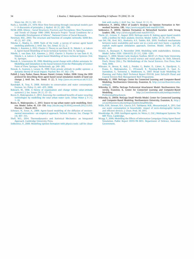
I. Koutiva, C. Makropoulos / Environmental Modelling & Software 79 (2016) 35e5454
Water Int. 29 (1), 105e113.Nash, J., Sutcliffe, J.V., 1970. River flow forecasting through conceptual models part
IdA discussion of principles. J. Hydrol. 10 (3), 282e290.NCSR, 2006. Athens - Social Structures, Practices and Perceptions: New Parameters
and Trends of Change 1980e2000, Research Project “Social Conditions for aSustainable Development of Athens”. National Centre of Social Research.
Newman, M.E., 2003. The structure and function of complex networks. SIAM Rev.45 (2), 167e256.
Nikolai, C., Madey, G., 2009. Tools of the trade: a survey of various agent basedmodeling platforms. J. Artif. Soc. Soc. Simul. 12 (2), 2.
Nikolic, I., Kasmire, J., 2012. Charter 2. Theory in van Dam K. H., Nikolic I., & LukszoZ, Agent-based Modelling of Socio-technical Systems (Vol. 9). Springer.
Nikolic, I., van Dam, K.H., Kasmire, J., 2012. Charter 3. Practice in van Dam K. H.,Nikolic I., & Lukszo Z, Agent-based Modelling of Socio-technical Systems (Vol.9). Springer.
Nowak, A., Lewenstein, M., 1996. Modeling social change with cellular automata. In:Modelling and Simulation in the Social Sciences from the Philosophy of SciencePoint of View. Springer, Netherlands, pp. 249e285.
Nowak, A., Szamrej, J., Latane, B., 1990. From private attitude to public opinion: adynamic theory of social impact. Psychol. Rev. 97, 362e376.
Polhill, J. Gary, Parker, Dawn, Brown, Daniel, Grimm, Volker, 2008. Using the ODDprotocol for describing three agent-based social simulation models of land-usechange. J. Artif. Soc. Soc. Simul. 11 (2), 3. http://jasss.soc.surrey.ac.uk/11/2/3.html.
Randolph, B., Troy, P., 2008. Attitudes to conservation and water consumption.Environ. Sci. Policy 11, 441e455, 2008.
Rokeach, M., 1968. A theory of organization and change within value-attitudesystems1. J. Soc. Issues 24 (1), 13e33.
Rozos, E., Makropoulos, C., 2012. Assessing the combined benefits of water recyclingtechnologies by modelling the total urban water cycle. Urban Water J. 9 (1),1e10.
Rozos, E., Makropoulos, C., 2013. Source to tap urban water cycle modelling. Envi-ron. Model. Softw. 41, 139e150. http://dx.doi.org/10.1016/j.envsoft.2012.11.015.Elsevier, 1 March 2013.
Schwarz, N., Ernst, A., 2009. Agent-based modeling of the diffusion of environ-mental innovationsdan empirical approach. Technol. Forecast. Soc. Change 76(4), 497e511.
Shell, M.S., 2014. Thermodynamics and Statistical Mechanics: an IntegratedApproach. Cambridge University Press.
Sobkowicz, P., 2009. Modelling opinion formation with physics tools: call for closer
link with reality. J. Artif. Soc. Soc. Simul. 12 (1), 11.Sobkowicz, P., 2003a. Effect of Leader's Strategy on Opinion Formation in Net-
worked Societies. URL. http://arxiv.org/pdf/cond-mat/0311566.Sobkowicz, P., 2003b. Opinion Formation in Networked Societies with Strong
Leaders. URL. http://arxiv.org/pdf/cond-mat/0311521.Thiele, J.C., Grimm, V., August 2010. NetLogo meets R: linking agent-based models
with a toolbox for their analysis. Environ. Model. Softw. 25 (8), 972e974.van Oel, P.R., Krol, M.S., Hoekstra, A.Y., Taddei, R.R., 2010. Feedback mechanisms
between water availability and water use in a semi-arid river basin: a spatiallyexplicit multi-agent simulation approach. Environ. Model. Softw. 25 (4),433e443.
Voinov, A., Bousquet, F., November 2010. Modelling with stakeholders. Environ.Model. Softw. ISSN: 1364-8152 25 (11), 1268e1281.
Wagener, T., 2004. Monte Carlo Analysis Toolbox, MCAT v.5. Penn State University.Weber, M., 1904. Objectivity of social science and social policy. In: Shils, Edward,
Finch, Henry (Eds.), The Methodology of the Social Sciences. Free Press, NewYork, 1949.
Wheater, H., Beven, K., Hall, J., Pender, G., Butler, D., Calver, A., Djordjevic, S.,Evans, E., Makropoulos, C., O'Connell, E., Penning-Rowsell, E., Saul, A.,Surendran, S., Townend, I., Watkinson, A., 2007. Broad Scale Modelling forPlanning and Policy R&D Technical Report FD2118, Joint Defra/EA Flood andCoastal Erosion Risk Management R&D Programme.
Wilensky, U., 1999. NetLogo. Center for Connected Learning and Computer-BasedModeling, Northwestern University, Evanston, IL. http://ccl.northwestern.edu/netlogo/.
Wilensky, U., 2005a. NetLogo Preferential Attachment Model. Northwestern Uni-versity, Evanston, IL. Center for Connected Learning and Computer-BasedModelling. http://ccl.northwestern.edu/netlogo/models/PreferentialAttachment.
Wilensky, U., 2005b. NetLogo Small Worlds Model. Center for Connected Learningand Computer-Based Modeling, Northwestern University, Evanston, IL. http://ccl.northwestern.edu/netlogo/models/SmallWorlds.
Willis, R.M., Stewart, R.A., Giurco, D.P., Talebpour, M.R., Mousavinejad, A., 2011. Enduse water consumption in households: impact of socio-demographic factorsand efficient devices. J. Clean. Prod. 30, 2011.
Wooldridge, M., 1999. Intelligent agents. In: Weiss, G. (Ed.), Multiagent Systems. TheMIT Press, Cambridge.
Wragg, T., 2006. Modelling the Effects of Information Campaigns Using Agent BasedSimulation, Public Report DSTO-TR-1853. Department of Defence, AustralianGovernment.