HAL Id: hal-01252122https://hal.inria.fr/hal-01252122

Submitted on 7 Jan 2016

HAL is a multi-disciplinary open accessarchive for the deposit and dissemination of sci-entific research documents, whether they are pub-lished or not. The documents may come fromteaching and research institutions in France orabroad, or from public or private research centers.

L’archive ouverte pluridisciplinaire HAL, estdestinée au dépôt et à la diffusion de documentsscientifiques de niveau recherche, publiés ou non,émanant des établissements d’enseignement et derecherche français ou étrangers, des laboratoirespublics ou privés.

Modelling interactions between tumour cells andsupporting adipocytes in breast cancer

Camille Pouchol

To cite this version:Camille Pouchol. Modelling interactions between tumour cells and supporting adipocytes in breastcancer. Mathematics [math]. 2015. <hal-01252122>

Modelling interactions between tumour cells and supportingadipocytes in breast cancer

Camille Pouchol, under the supervision of Jean Clairambault

Internship report

Contents

1 Breast cancer and its environment 41.1 Breast cancer : a brief overview . . . . . . . . . . . . . . . . . . . . . . . . . . . . 4

1.1.1 Some statistics in France . . . . . . . . . . . . . . . . . . . . . . . . . . . . 41.1.2 Location of breast cancers . . . . . . . . . . . . . . . . . . . . . . . . . . . 41.1.3 Different types of breast cancers . . . . . . . . . . . . . . . . . . . . . . . 51.1.4 Therapeutics for breast cancer . . . . . . . . . . . . . . . . . . . . . . . . 5

1.2 Interactions between the tumour and the adipose tissue . . . . . . . . . . . . . . 51.2.1 Short description of the adipose tissue . . . . . . . . . . . . . . . . . . . . 51.2.2 Mutualistic interactions . . . . . . . . . . . . . . . . . . . . . . . . . . . . 6

1.3 The key role of adipocytes . . . . . . . . . . . . . . . . . . . . . . . . . . . . . . . 61.3.1 In cell proliferation . . . . . . . . . . . . . . . . . . . . . . . . . . . . . . . 71.3.2 In invasive phenotype . . . . . . . . . . . . . . . . . . . . . . . . . . . . . 71.3.3 In resistance to therapy . . . . . . . . . . . . . . . . . . . . . . . . . . . . 8

2 Experimental setting and mathematical modelling 92.1 Experimental setting . . . . . . . . . . . . . . . . . . . . . . . . . . . . . . . . . . 9

2.1.1 Principle and cell lines . . . . . . . . . . . . . . . . . . . . . . . . . . . . . 92.1.2 Estimating cell proliferation and distribution in phenotypes . . . . . . . . 9

2.2 Mathematical modelling . . . . . . . . . . . . . . . . . . . . . . . . . . . . . . . . 102.2.1 Underlying principles . . . . . . . . . . . . . . . . . . . . . . . . . . . . . . 102.2.2 Typical equation . . . . . . . . . . . . . . . . . . . . . . . . . . . . . . . . 112.2.3 Equation for the interaction between adipocytes and cancer cells . . . . . 11

3 Single integro-differential equation 133.1 Existence and uniqueness . . . . . . . . . . . . . . . . . . . . . . . . . . . . . . . 13

3.1.1 A priori bounds . . . . . . . . . . . . . . . . . . . . . . . . . . . . . . . . . 143.1.2 Proof of existence and uniqueness . . . . . . . . . . . . . . . . . . . . . . . 14

3.2 Asymptotics . . . . . . . . . . . . . . . . . . . . . . . . . . . . . . . . . . . . . . . 153.2.1 Convergence for ρ . . . . . . . . . . . . . . . . . . . . . . . . . . . . . . . 153.2.2 Convergence for n . . . . . . . . . . . . . . . . . . . . . . . . . . . . . . . 16

4 System of two integro-differential equations 184.1 Mutualistic 2 × 2 Lotka-Volterra systems . . . . . . . . . . . . . . . . . . . . . . 18

4.1.1 Possible blow-up . . . . . . . . . . . . . . . . . . . . . . . . . . . . . . . . 194.1.2 Convergence in the case (24) . . . . . . . . . . . . . . . . . . . . . . . . . 19

4.2 Existence and uniqueness . . . . . . . . . . . . . . . . . . . . . . . . . . . . . . . 204.2.1 Regularity and non blow-up assumptions . . . . . . . . . . . . . . . . . . . 204.2.2 A priori bounds for ρ1 and ρ2 . . . . . . . . . . . . . . . . . . . . . . . . . 21

1

4.2.3 Existence and uniqueness . . . . . . . . . . . . . . . . . . . . . . . . . . . 234.3 Asymptotics . . . . . . . . . . . . . . . . . . . . . . . . . . . . . . . . . . . . . . . 24

4.3.1 Convergence for ρ1 and ρ2 . . . . . . . . . . . . . . . . . . . . . . . . . . . 24

5 Parametrization of the model 255.1 With explicit formulas . . . . . . . . . . . . . . . . . . . . . . . . . . . . . . . . . 25

5.1.1 Main ideas and model simplification . . . . . . . . . . . . . . . . . . . . . 255.1.2 Explicit formulas . . . . . . . . . . . . . . . . . . . . . . . . . . . . . . . . 26

5.2 By means of numerical simulations . . . . . . . . . . . . . . . . . . . . . . . . . . 275.2.1 Numerical scheme . . . . . . . . . . . . . . . . . . . . . . . . . . . . . . . 275.2.2 Examples of results . . . . . . . . . . . . . . . . . . . . . . . . . . . . . . . 28

A BV functions on R+ 30

B Handling positive and negative parts for ODEs 30

C Computations for the explicit solution to the equation on R 31

References 35

2

This internship report on the subject "Modelling interactions between tumour cells and sup-porting adipocytes in breast cancer", is a summary of the work accomplished during 6 monthsof internship at the Laboratoire Jacques-Louis-Lions (LJLL). Since this internship is intendedto be followed by a PhD on the same subject, most of the work was bibliographical and aimedat understanding the biological background, the modelling and analysis of phenotypically struc-tured populations, as well as the envisaged experiments, that are performed at the Laboratoirede Biologie et Thérapeutique des Cancers (LBTC) in Michèle Sabbah’s team. Those experi-ments will allow for validation and parametrization of the models. An other part of the workwas to start proving new mathematical results, and perform numerical simulations to investigatedifferent scenarios.

Introduction

In breast cancer, invasion of the micro-environment implies potential bidirectional communica-tion between cancer cells and the adipose tissue. Biological evidence suggests that adipocytes,in particular, are key-actors in tumorigenesis and invasion: they both enhance proliferation ofthe cancer cells and favor acquisition of a more invasive phenotype. To understand these effects,mathematical modelling (thanks to tools developed in theoretical ecology) is used to performasymptotic analysis in number of cells and distribution of phenotypes. These models can betuned through confrontation with experimental data coming from co-cultures of cancer cellswith adipocytes.The first part of this report is devoted to presenting the biological background on breast cancerand its environment. We then present the main aspects of the mathematical modelling, andhow it is expected to be validated experimentally. In the third part, we summarize and provemany important results that have been obtained on a single integro-differential equation rep-resenting the evolution of a population of individuals structured with a phenotypic trait. Thenext part consists of a first glance at possible generalizations of those results to a system ofintegro-differential equations coupled mutualistically. In a fifth and last part, we introduce howwe intend to parametrize the models through explicit computations and numerical simulations.

3

1 Breast cancer and its environment

1.1 Breast cancer : a brief overview

1.1.1 Some statistics in France

What follows is a summary from a survey issued by the IVS (Institut de Veille Sanitaire). Thestatistics are taken from the year 2012, exclusively in France. Note that the incidence andmortality figures have been roughly stable for the last decade.In France, in 2012, around 50, 000 new cases were reported, for around 10, 000 deaths. Onewoman out of eight will have breast cancer at some time in life. After 5 years, the survival rateis about 86% (all types included). Age is a strong factor, as 45% of breast cancers are diagnosedbetween 50 and 69 years and around 33% after 69 years.

1.1.2 Location of breast cancers

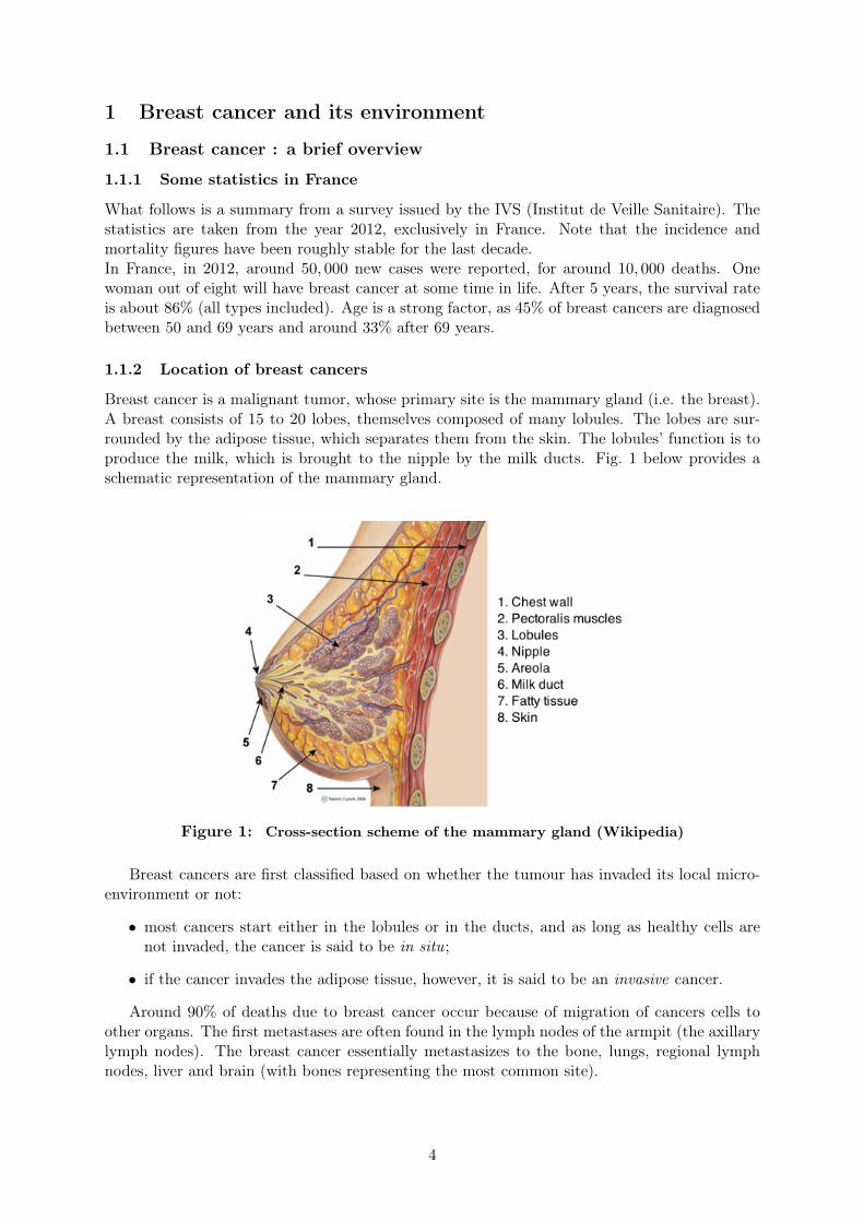
Breast cancer is a malignant tumor, whose primary site is the mammary gland (i.e. the breast).A breast consists of 15 to 20 lobes, themselves composed of many lobules. The lobes are sur-rounded by the adipose tissue, which separates them from the skin. The lobules’ function is toproduce the milk, which is brought to the nipple by the milk ducts. Fig. 1 below provides aschematic representation of the mammary gland.

Figure 1: Cross-section scheme of the mammary gland (Wikipedia)

Breast cancers are first classified based on whether the tumour has invaded its local micro-environment or not:

• most cancers start either in the lobules or in the ducts, and as long as healthy cells arenot invaded, the cancer is said to be in situ;

• if the cancer invades the adipose tissue, however, it is said to be an invasive cancer.

Around 90% of deaths due to breast cancer occur because of migration of cancers cells toother organs. The first metastases are often found in the lymph nodes of the armpit (the axillarylymph nodes). The breast cancer essentially metastasizes to the bone, lungs, regional lymphnodes, liver and brain (with bones representing the most common site).

4

1.1.3 Different types of breast cancers

Depending on the involved cancer cells’ phenotype, two breast cancers can differ drastically, andthis has very important implications in terms of therapeutical strategies and life expectancy. Tocover the most prevalent types, it is enough to characterize a cancer cell based on the presence(+) of absence (−) of:

• hormone receptors for estrogens (ER) and progesterone (PR);

• the gene HER2, responsible for over-expression of the growth-promoting protein HER2.

From that, it is possible to distinguish 3 types of breast cancers:

• Luminal A (ER+, PR+, HER2-) and B (ER+, PR-, HER2+) → 70%;

• HER2 positive (ER-, PR- , HER2+) → 15%;

• "triple-negative" or "basal-like" (ER-, PR-, HER2-) → 15%,

where the percentages indicate the approximate contribution of each type to the total numberof breast cancers in France (data taken from the Curie Institute website).

1.1.4 Therapeutics for breast cancer

As for other cancers, clinical treatment of breast cancers consists of several approaches than canbe combined. The choice of one or several therapies, as well as their scheduling and duration,depends on a wide variety of factors, including which the type of cancer, its location (invasive ornot, metastases), the size of the different tumors and, of course, the health status of the patient.One can identify 5 main approaches for a clinician facing a breast cancer:

• chemotherapyChemotherapy refers to chemical drugs that kill the cancer cells (cytotoxic effect) and/or blocktheir proliferation (cytostatic effect). These are often very toxic drugs, which can also affecthealthy cells.• surgery

Cancer surgery is the removal of (part of) the tumor and its surrounding tissues.• radiotherapy

Radiotherapy uses high-energy rays to target the cancer cells.• antiangiogenic drugs

When a tumor grows, the cells at the center cannot access nutrients anymore and become qui-escent (they stop dividing, waiting for better conditions). In those conditions, cancer cells areable to create their own vasculature, ensuring access to nutrients and potential migration. Thisis called angiogenesis, a process specifically targeted by antiangiogenic drugs.• blocking interactions between the tumor and its environment

Although the immune system can fight cancer, cancer cells also use their environment to theiradvantage, so as to create better conditions for their survival and proliferation. In breast cancer,there are indeed mutualistic interactions between cancer cells and cells of the adipose tissue (seenext section).

1.2 Interactions between the tumour and the adipose tissue

1.2.1 Short description of the adipose tissue

The main role of adipose tissue is to serve as an energy depot. There are few main types of cellsin the adipose tissue, listed thereafter:• adipocytes

5

Adipocytes are round cells, the most represented cells of the adipose tissue. They confer it itsfunction, as adipocytes maintain an energy balance by storing excess fat and releasing it whenneeded in the form of fatty acids. They can also synthesize estrogens [12].• fibroblasts

Fibroblasts are more elliptical cells. They synthesize many proteins than can be found in theextra-cellular matrix (ECM), thus contributing to structuring the stroma and having a wound-healing function.• endothelial cells

Endothelial cells form a thin layer around the blood vessels.• macrophages

Macrophages are cells that engulf and digest (this is called phagocytosis) anything that doesnot have the types of proteins specific to the surface of healthy body cells on its surface.• preadipocytes

Preadipocytes are undifferentiated fibroblasts that can be stimulated to form adipocytes.

1.2.2 Mutualistic interactions

Epidemiological studies have shown a positive link between obesity and breast cancer, both interms of risk of developing the disease and poor prognosis once it has been diagnosed [2, 9], atleast for post-menopausal women. For pre-menopausal women, the latter also seems to holdtrue, while the former doesn’t: many studies find an negative association between obesity andrisk of developing the disease before menopause [9]. More precisely, obesity is linked to higherlikelihood of larger tumours, recurrence of the disease, and death.Those studies often use the BMI (body mass index) to define obesity, an index built as a measureof body fat. Thus, they provide strong evidence of existence of interactions between the tumourand the adipose tissue.

Furthermore, those conclusions also have biological support. First, obesity is associated with(subclinical) inflammation of the adipose tissue, a state of the micro-environment which has beenproven to favor cancer progression [13]. Secondly, obesity leads to over-expression of aromatase,and subsequently, the hormon it synthesizes: estrogen [14]. Estrogens increase proliferation ofER positive cancer cells. It is also noteworthy that most post-menopausal breast cancers areER positive.

Knowledge of such interactions already has applications in clinics: hormone therapy (drugsthat compete with estrogens for binding to estrogen receptors) and aromatase inhibitors areused. Nonsteroidal anti-inflammatory drugs are also used.

1.3 The key role of adipocytes

Among cells of the adipose tissue, recent biological evidence suggests that adipocytes play akey role in cell proliferation, invasive phenotype and resistance to therapy as far as cancer cellsare concerned. Adipocytes at the interface with the tumour exhibit a modified phenotype, andare now called Cancer-Associated Adipocytes (CAAs) [5,15]. They are indeed characterized bya much smaller size (see Fig. 2) due to delipidation and a lower expression of adiponectin (acytokine emitted by mature adipocytes).

6

Figure 2: Histology of the invasive front of a human breast carcinoma. Data reproducedfrom [15]. In white: adipocytes, in purple: tumour.

1.3.1 In cell proliferation

When cultured in a medium containing soluble factors emitted by adipocytes, cancer cells aresignificantly more proliferative, a conclusion that does not hold if the factors are emitted byfibroblasts [7]. Similar conclusions are obtained in terms of cell proliferation in the case ofcancer cells cultured with adipocytes in a three-dimensional collagen gel matrix [10].

1.3.2 In invasive phenotype

Epithelial to mesenchymal transition (EMT) is a reversible process by which epithelial cellspartly lose their adherent properties (and their polarity), and thus become more motile. Thistransition is known to occur in cancer cells, and is strongly related to invasive properties of thecancer, and metastases. Put in contact with adipocytes through soluble factors only, cancer cellsundergo the EMT [5], proving that adipocytes are linked to cancer invasion. Together with thechange of adipocytes from mature adipocytes (A) to CAAs, this shows that crosstalk betweenboth populations change their phenotype, a situation summarized in Fig. 3.

Figure 3: Bidirectional communication between adipocytes and cancer cells induce achange of phenotypes in both populations. E: epithelial, M: mesenchymal, A: (mature) adipocytes,CAA: cancer-associated adipocytes.

7

1.3.3 In resistance to therapy

Different biological studies have shown that, under the influence of adipocytes, cancer cells candevelop a resistance to different therapies.In [1] the authors show that cancer cells co-cultured with adipocytes have become resistantto radiotherapy. This effect is independent of whether cancer cells are left in co-culture withadipocytes, or not (at least on a window of 2 days).In [6], cancer cells expressing HER2 (HER2+) are found to develop resistance to trastuzumab-mediated cytotoxicity (trastuzumab is a drug that blocks the extra-cellular part of the receptorfor HER2) if co-cultured with adipocytes or preadipocytes.

8

2 Experimental setting and mathematical modelling

To further study the interactions between cancer cells and adipocytes, the goal is to performexperiments of co-culture of cancer cells with adipocytes. Mathematical modelling can thenserve as an in silico laboratory to guide experiments and investigate scenarios that are notdirectly accessible, or too costly.

2.1 Experimental setting

2.1.1 Principle and cell lines

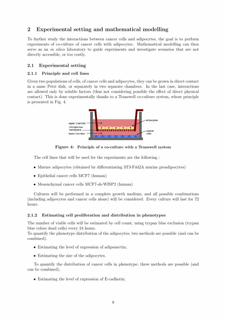
Given two populations of cells, of cancer cells and adipocytes, they can be grown in direct contactin a same Petri dish, or separately in two separate chambers. In the last case, interactionsare allowed only by soluble factors (thus not considering possible the effect of direct physicalcontact). This is done experimentally thanks to a Transwell co-culture system, whose principleis presented in Fig. 4.

Figure 4: Principle of a co-culture with a Transwell system

The cell lines that will be used for the experiments are the following :

• Mature adipocytes (obtained by differentiating 3T3-F442A murine preadipocytes)

• Epithelial cancer cells MCF7 (human)

• Mesenchymal cancer cells MCF7-sh-WISP2 (human)

Cultures will be performed in a complete growth medium, and all possible combinations(including adipocytes and cancer cells alone) will be considered. Every culture will last for 72hours.

2.1.2 Estimating cell proliferation and distribution in phenotypes

The number of viable cells will be estimated by cell count, using trypan blue exclusion (trypanblue colors dead cells) every 24 hours.To quantify the phenotype distribution of the adipocytes, two methods are possible (and can becombined).

• Estimating the level of expression of adiponectin;

• Estimating the size of the adipocytes.

To quantify the distribution of cancer cells in phenotype, three methods are possible (andcan be combined).

• Estimating the level of expression of E-cadherin;

9

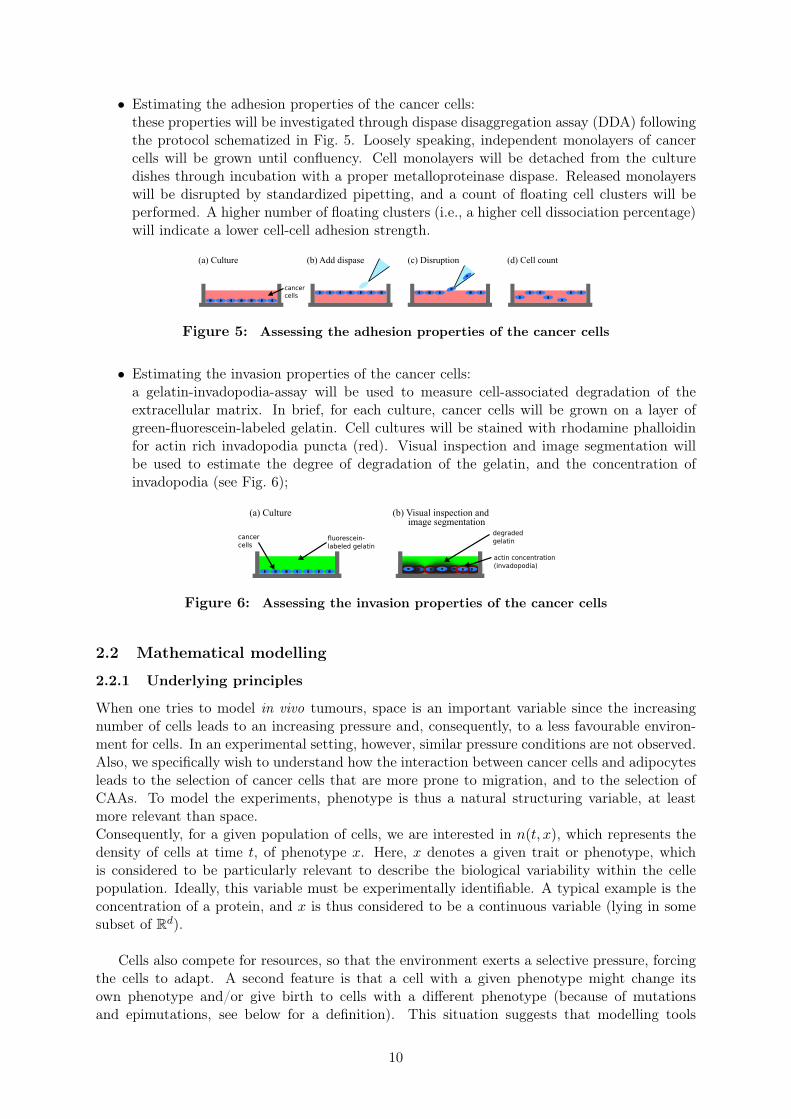
• Estimating the adhesion properties of the cancer cells:these properties will be investigated through dispase disaggregation assay (DDA) followingthe protocol schematized in Fig. 5. Loosely speaking, independent monolayers of cancercells will be grown until confluency. Cell monolayers will be detached from the culturedishes through incubation with a proper metalloproteinase dispase. Released monolayerswill be disrupted by standardized pipetting, and a count of floating cell clusters will beperformed. A higher number of floating clusters (i.e., a higher cell dissociation percentage)will indicate a lower cell-cell adhesion strength.

���������������������������������������������������������������������������������������������� � ����������������������������������������������������������� �����������

�����������

Figure 5: Assessing the adhesion properties of the cancer cells

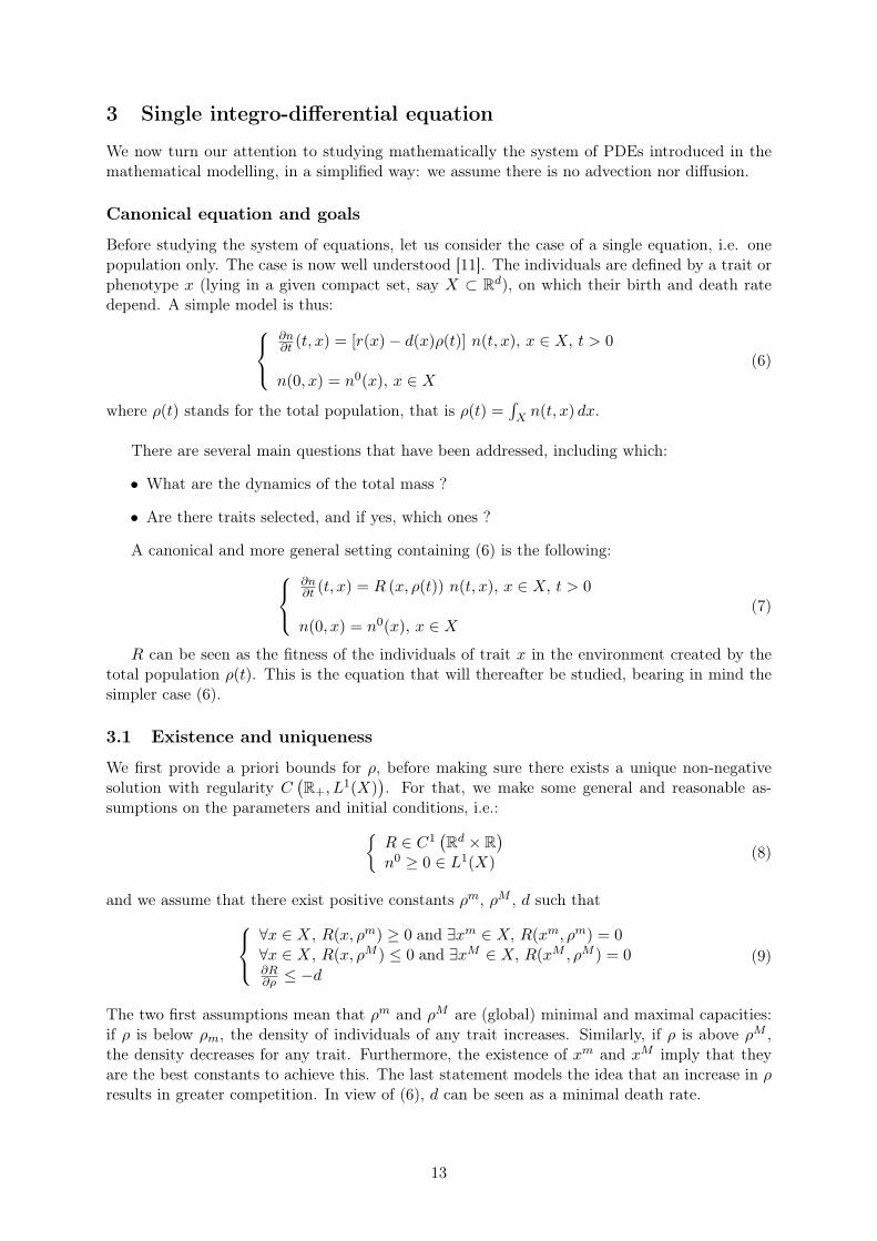
• Estimating the invasion properties of the cancer cells:a gelatin-invadopodia-assay will be used to measure cell-associated degradation of theextracellular matrix. In brief, for each culture, cancer cells will be grown on a layer ofgreen-fluorescein-labeled gelatin. Cell cultures will be stained with rhodamine phalloidinfor actin rich invadopodia puncta (red). Visual inspection and image segmentation willbe used to estimate the degree of degradation of the gelatin, and the concentration ofinvadopodia (see Fig. 6);

�����������

������������������������������������������������������������������������������������������������������������� ����� ����� ������������������������ ����������� ��

������������ ������������

���������������

����������������������������

Figure 6: Assessing the invasion properties of the cancer cells

2.2 Mathematical modelling

2.2.1 Underlying principles

When one tries to model in vivo tumours, space is an important variable since the increasingnumber of cells leads to an increasing pressure and, consequently, to a less favourable environ-ment for cells. In an experimental setting, however, similar pressure conditions are not observed.Also, we specifically wish to understand how the interaction between cancer cells and adipocytesleads to the selection of cancer cells that are more prone to migration, and to the selection ofCAAs. To model the experiments, phenotype is thus a natural structuring variable, at leastmore relevant than space.Consequently, for a given population of cells, we are interested in n(t, x), which represents thedensity of cells at time t, of phenotype x. Here, x denotes a given trait or phenotype, whichis considered to be particularly relevant to describe the biological variability within the cellepopulation. Ideally, this variable must be experimentally identifiable. A typical example is theconcentration of a protein, and x is thus considered to be a continuous variable (lying in somesubset of Rd).

Cells also compete for resources, so that the environment exerts a selective pressure, forcingthe cells to adapt. A second feature is that a cell with a given phenotype might change itsown phenotype and/or give birth to cells with a different phenotype (because of mutationsand epimutations, see below for a definition). This situation suggests that modelling tools

10

provided by mathematical ecology (and more particularly, adaptive dynamics) can be used. Thisbranch of mathematical biology focuses on understanding mathematically how selection occursin a population of individuals interacting between themselves and with their environment (in acompetitive and/or mutualistic way), and subject to mutations and epimutations [4, 8, 11].

2.2.2 Typical equation

Let us now introduce a prototype equation (coming from adaptive dynamics) describing theevolution of a population of cells defined by n(t, x). Close models can for example be foundin [3, 8, 11]. For simplicity, we will assume that the trait lies in some sub-interval of R, sayX := [0 , 1]. The equation for n is given by:

∂n

∂t(t, x) +

∂

∂x(v(x)n(t, x)) = β

∂2n

∂x2(t, x) +R (x, ρ(t))n(t, x). (1)

with initial condition n0 ≥ 0 in L1(X) ∩ L∞(X) and Neumann boundary conditions. We alsoassume that the adaptation velocity v vanishes at the boundary.

Each term models a different phenomenon:

• The R (x, ρ(t))n(t, x) term.R is a fitness function for the cells of phenotype x in the environment created by thetotal population (which is modelled by the dependence in the total population given byρ(t) :=

∫X n(t, x) dx). The most common example is

R (x, ρ(t)) = r(x)− d(x)ρ(t) (2)

which amounts to saying that cells give birth at rate r(x) and die at rate d(x)ρ(t). Thedependence in ρ is of logistic type, representing the idea that cells die faster when the totalpopulation is bigger, because of competition for nutrients and space.

• The β∂2n

∂x2(t, x) term

The Laplacian models random epimutations, i.e. random heritable gene expressions thatleaves the DNA unaffected. β quantifies the rate of epimutations. Note that we do nottake mutations into account (usually modelled with a probability kernel) because they aresupposed to occur much less frequently. They are thus here neglected.Such a term can be called of Darwin-type, since it implies that the emergence or selectionof fitter individuals occurs because of random events.

• The∂

∂x(v(x)n(t, x)) term

This advection term means that the density is transported with velocity v(x). It modelsnon-random epimutations.Such a term can be called of Lamarck-type, since it implies that the emergence or selectionof fitter individuals occurs because these individuals actively change their phenotype toadapt to their environment.

2.2.3 Equation for the interaction between adipocytes and cancer cells

To model the experiments of co-culture between cancer cells and adipocytes, we are interested inthe behaviour of the two population densities nC(t, x) (cancer cells) and nA(t, y) (adipocytes).x and y stand for traits that characterize the phenotype of the individuals:

• for cancer cells, x ranges from 0 for an epithelial phenotype E to 1 for a mesenchymalphenotype M. x can be linked to the concentration of a protein through a proper normal-ization;

11

• for adipocytes, y ranges from 0 for mature adipocytes A to 1 for cancer-associated adipocytesCAA. y can be linked to the concentration of a protein through a proper normalization.

Figure 7: Meaning of the traits x and y.

We consider the following set of PDEs

∂nC∂t

(t, x) +∂

∂x(vC (x, ϕA(t))nC(t, x))

= βC∂2nC∂x2

+ [RC (x, ρC(t)) +RCA (x, ϕA(t))]nC(t, x)

∂nA∂t

(t, y) +∂

∂y(vA (y, ϕC(t))nA(t, y))

= βA∂2nA∂y2

+ [RA (y, ρA(t)) +RAC (y, ϕC(t))]nA(t, y)

(3)

with initial conditions depending on the experiment and Neumann boundary conditions.The interaction is modelled through dependence of different terms on functions ϕA and ϕC ,which aim at representing the chemical signal from adipocytes to cancer cells (resp. from cancercells to adipocytes). A possible definition is{

ϕC(t) =∫ 1

0 ψC(x)nC(t, x) dx

ϕA(t) =∫ 1

0 ψA(y)nA(t, y) dy(4)

with ψC , ψA increasing functions (modelling the fact that mesenchymal cells or CAAsare expected to emit more chemical messengers than, respectively, epithelial cells and matureadipocytes).

The interactions impact two terms:

• The RCA (x, ϕA(t))nC(t, x) and RAC (y, ϕC(t))nA(t, y) terms.Since the interaction is mutualistic in terms of cell proliferation (at least for cancer cells),we assume that RCA (x, ϕA) ≥ 0 with equality if and only if ϕA = 0 and, possibly,RAC (y, ϕC) ≥ 0 with equality if and only if ϕC = 0. Typically, we will take

RCA (x, ϕA) = sC(x)ϕA (5)

with sC(x) ≥ 0 the sensitivity of cancer cells to the chemical messengers. Note that thepopulation of adipocytes can be seen as inducing an added birth rate for the cancer cells.

• The∂

∂x(vC (x, ϕA(t))nC(t, x)) and

∂

∂y(vA (y, ϕC(t))nA(t, y)) terms

We still assume that vC and vA vanish at the boundary (independently of the value of ϕAand ϕC respectively) for well-posedness.Since cancer cells tend to naturally undergo the epithelial to mesenchymal transition, weassume vC ≥ 0. Since the interaction tends to lead to a change of phenotype from E toM and A to CAA, we also assume that vC and vA are increasing functions of ϕA and ϕC ,respectively.

12

3 Single integro-differential equation

We now turn our attention to studying mathematically the system of PDEs introduced in themathematical modelling, in a simplified way: we assume there is no advection nor diffusion.

Canonical equation and goals

Before studying the system of equations, let us consider the case of a single equation, i.e. onepopulation only. The case is now well understood [11]. The individuals are defined by a trait orphenotype x (lying in a given compact set, say X ⊂ Rd), on which their birth and death ratedepend. A simple model is thus:

∂n∂t (t, x) = [r(x)− d(x)ρ(t)] n(t, x), x ∈ X, t > 0

n(0, x) = n0(x), x ∈ X(6)

where ρ(t) stands for the total population, that is ρ(t) =∫X n(t, x) dx.

There are several main questions that have been addressed, including which:

• What are the dynamics of the total mass ?

• Are there traits selected, and if yes, which ones ?

A canonical and more general setting containing (6) is the following:∂n∂t (t, x) = R (x, ρ(t)) n(t, x), x ∈ X, t > 0

n(0, x) = n0(x), x ∈ X(7)

R can be seen as the fitness of the individuals of trait x in the environment created by thetotal population ρ(t). This is the equation that will thereafter be studied, bearing in mind thesimpler case (6).

3.1 Existence and uniqueness

We first provide a priori bounds for ρ, before making sure there exists a unique non-negativesolution with regularity C

(R+, L

1(X)). For that, we make some general and reasonable as-

sumptions on the parameters and initial conditions, i.e.:{R ∈ C1

(Rd × R

)n0 ≥ 0 ∈ L1(X)

(8)

and we assume that there exist positive constants ρm, ρM , d such that∀x ∈ X, R(x, ρm) ≥ 0 and ∃xm ∈ X, R(xm, ρm) = 0∀x ∈ X, R(x, ρM ) ≤ 0 and ∃xM ∈ X, R(xM , ρM ) = 0∂R∂ρ ≤ −d

(9)

The two first assumptions mean that ρm and ρM are (global) minimal and maximal capacities:if ρ is below ρm, the density of individuals of any trait increases. Similarly, if ρ is above ρM ,the density decreases for any trait. Furthermore, the existence of xm and xM imply that theyare the best constants to achieve this. The last statement models the idea that an increase in ρresults in greater competition. In view of (6), d can be seen as a minimal death rate.

13

3.1.1 A priori bounds

Lemma 3.1. Suppose we have a solution of (7) in C(R+, L

1(X)), with the initial data such

that ρm ≤ ρ0 :=∫X n0(x) dx ≤ ρM .

Then, for all t > 0:

ρm ≤ ρ(t) ≤ ρM .

Proof. Integrating the equation yields, for all t ≥ 0:

dρ

dt(t, x) ≤

[maxx∈X

R (x, ρ(t))

]ρ(t)

Let ε > 0. If ρ(t) is close to ρM + ε, its derivative becomes negative and this is enough to ensureρ(t) ≤ ρM + ε for all t > 0. We then let ε go to 0 to get the upper bound.The same arguments provide the other inequality.

3.1.2 Proof of existence and uniqueness

First, we notice that we have an implicit formula for n(t, x):

n(t, x) = n0(x)e∫ t0 R(x,ρ(s)) ds (10)

which shows that n is necessarily non-negative.

Theorem 3.2. Assume, as in Lemma (3.1), that n0 is such that ρm ≤ ρ0 :=∫X n0(x) dx ≤ ρM .

Then, there exists a unique non-negative global solution n to the equation (7).It furthermore satisfies:

ρm ≤ ρ(t) ≤ ρM for all t > 0.

Proof. The proof is based on the Banach fixed point theorem.

First step. We start by defining the appropriate Banach space. For T > 0 that will be chosenlater, we consider the Banach space

E := C([0 , T ], L1(X)

)endowed with the norm ‖m‖E := sup

0≤t≤T‖m(t)‖L1(X)

We also consider the following closed subset of E:

F := {m ∈ E /m ≥ 0 and ‖m‖E ≤ K}

where K > ρM is some constant.

Second step. We now build the application. Let m be a fixed element in F , and let us define

ρ̃(t) =

∫Xm(t, x) dx

For fixed x0 ∈ X, we consider the solution γx0 to the following differential equation:{dγx0dt = R (x, ρ̃(t)) γx0γx0(0) = n0(x0)

which is global on [0 , T ]. 1

1Note that this function is defined as an integral of m, and thus does not depend on the representative for thea.e. equivalence relation.

14

We now define for all (t, x) in [0 , T ] × X the function n(t, x) := γx(t), thus building anapplication Φ through Φ(m) := n.

Third step. We show that Φ maps F onto itself.The equation (3.1.2) can be solved explicitly by

n(t, x) = n0(x)e∫ t0 R(x,ρ̃(s)) ds

It shows both n ≥ 0 and n ∈ E. As in the a priori estimates, we bound ∂n∂t (t, x) and integrate

to get

dρ

dt(t) ≤

[maxx∈X

R (x, ρ̃(t))

]ρ(t)

Using the bound on the initial data, together with maxx∈X

R (x, ρ̃(t)) ≤ maxx∈X

R (x, 0) =: λ, weget

ρ(t) ≤ ρMeλT

To obtain n ∈ F , it only remains to choose T small enough so that ρMeλT ≤ K.

Fourth step. Let us now prove that Φ is a strong contraction from F onto F whenever T issmall enough. Let (m1,m2) ∈ F 2 and (n1, n2) its image by Φ. We define ρ̃i as before for i = 1, 2.

(n1 − n2)(t, x) = n0(x)[e∫ t0 R(x,ρ̃1(s)) ds − e

∫ t0 R(x,ρ̃2(s)) ds

]Now, since the argument of the exponentials can be bounded by λT , the mean value theoremyields

|(n1 − n2)|(t, x) ≤ n0(x)eλT∣∣∣∣∫ t

0

[R(x, ρ̃1(s)

)−R

(x, ρ̃2(s)

)]ds

∣∣∣∣≤ Cn0(x)eλT

[∫ T

0

∣∣ρ̃1(s)− ρ̃2(s)∣∣ ds ds]

≤ Cn0(x)TeλT ‖m1 −m2‖E (11)

by the mean value theorem again, with C := sup(x,ρ)∈X×[0 ,K]

∣∣∂R∂ρ (x, ρ)

∣∣. We now integratewith respect to x and take the supremum over t ∈ [0 , T ] in (11) to uncover

‖n1 − n2‖E ≤ CρMTeλT ‖m1 −m2‖EThis provides us with the contracting property for Φ whenever T is small enough.

Fifth step. We now conclude by noticing that T has been chosen small independently of theinitial data, so that the argument can be iterated on [0 , T ], [T , 2T ], etc.By the a priori estimates of the lemma, we also iteratively have the bounds stated in thetheorem.

3.2 Asymptotics

3.2.1 Convergence for ρ

The previous hypotheses are enough to show that ρ converges. It is also possible to identify thelimit as the maximal capacity ρM , if we simply assume the following: among the xM s such thatR(xM , ρM ) = 0, there exists x0 such that n0 does not vanish in a neighborhood of x0.Note that this is not really a restriction, since we can for example assume that n0 is continuous,so that n0(x0) > 0 would be enough for our purpose (and if it were not true, we could definethe set X and ρM differently, removing the traits for which n0 is zero).

To show that ρ converges, we will prove that it has bounded total variation on R+ (see Ap-pendix A for a reminder of the fact that a BV function on R+ converges).

15

Proposition 3.3. ρ is a BV function and thus converges. Furthermore, its limit is ρM .

Proof. We define q :=dρ

dtand we need to prove that q ∈ L1(R+). We differentiate

dρ

dt=∫nR

to obtain:dq

dt=

∫nR2 +

(∫n∂R

∂ρ

)q

It provides an upper bound for the negative part of q (see Appendix B):

dq−dt≤(∫

n∂R

∂ρ

)q−

≤ −dρmq−

thanks to the hypothesis in (9) and the lower bound on ρ. We conclude that the negative partof q vanishes exponentially. Together with the upper bound on ρ, this proves the first result(see Appendix A for a proof that an upper bounded function whose derivative has integrablenegative part, is BV ).

We denote the limit with ρ?, and argue by contradiction by assuming ρ? < ρM .Let ε > 0 and t0 > 0 such that ρ(t) ≤ ρM − ε for all t > t0. Then, for x ∈ V a neighborhood ofx0 such that R(x0, ρ

M ) = 0 and t > t0, we can write

∂n

∂t(t, x) = R (x, ρ(t))n(t, x)

≥ R(x, ρM − ε

)n(t, x)

≥ η n(t, x)

for some η > 0 (choosing ε small enough). This now implies for t > t0

ρ(t) ≥∫Vn(t, x) dx ≥

[∫Vn0(x)

]eη(t−t0)

which contradicts the upper bound on ρ since the right hand side goes to +∞.

3.2.2 Convergence for n

We now assume that there exists a single trait x0 such that R(·, ρM ) vanishes, which meansthat one trait has a selective advantage over all others. Our aim is to prove that the populationasymptotically concentrates in x0. The idea is that for all the other traits, n(t, x) goes to 0exponentially. The correct statement is given in the theorem hereafter:

Theorem 3.4. Suppose there is a unique trait x0 such that R(x0, ρM ) = 0. Then the population

concentrates in x0 with mass ρM , i.e.

n(t, x) ⇀ ρMδx0

Remark 3.5. By the weak convergence here, we mean in the sense of the bounded measuresM1(X), defined as the (topological) dual of C(X) (the set of continuous functions on X).

Proof. As explained in the remark, we have to show that

∀φ ∈ C(X),

∫Xn(t, x)φ(x) dx→ ρMφ(x0)

Note that we already know, by the Banach-Alaoglu theorem, that we have converging sub-sequences since ∀t ≥ 0, ‖n(t, ·)‖L1(X) ≤ ρM : the family (n(t, ·))t≥0 is thus uniformly bounded

16

in M1(X). Here, we won’t use this result as we can directly determine the limit.

Let φ ∈ C(X). From∣∣∣∣∫Xn(t, x)φ(x) dx− ρMφ(x0)

∣∣∣∣ ≤ ∣∣∣∣∫Xn(t, x)φ(x) dx− φ(x0)

∫Xn(t, x) dx

∣∣∣∣+∣∣φ(x0)(ρ(t)− ρM )

∣∣ (12)

and since the last term goes to 0, it remains to show that the first one does as well.Let ε > 0. We choose η > 0 such that B(x0, η) ⊂ X and

∣∣φ(x) − φ(x0)∣∣ ≤ ε as soon as∣∣x− x0

∣∣ ≤ η, split the integral and estimate both terms:∣∣∣∣∫Xn(t, x)(φ(x)− φ(x0)) dx

∣∣∣∣ ≤ 2‖φ‖∞

(∫X\B(x0,η)

n(t, x) dx

)+ ρM ε (13)

As R(·, ρ) converges uniformly to R(·, ρM ) on X\B(x0, η) and maxx∈X\B(x0,η)R(·, ρM ) =:−α < 0, we can state that for t large enough, say t ≥ t0:

∀x ∈ X\B(x0, η), R(x, ρ) ≤ −α2

(14)

which allows us to write : n(t, x) ≤ n(t0, x)e−α2

(t−t0) on X\B(x0, η) from the equation on n.Therefore,

∫X\B(x0,η) n(t, x) dx goes to 0 and this completes the proof.

Remark 3.6. The proof also works if x0 does not lie in the interior of X, for example if X issome interval of R and if x0 is one of its extremities.

17

4 System of two integro-differential equations

Canonical equation and goals

We now wish to investigate the dynamics of the coupled equations (without advection anddiffusion), which we recall here with subscripts 1 and 2 rather than A and C. x can be taken asa variable for the traits structuring both populations, since they are independent.

∂n1

∂t(t, x) = [R1 (x, ρ1(t)) +R12 (x, ϕ2(t))]n1(t, x)x ∈ X, t > 0,

∂n2

∂t(t, x) = [R2 (x, ρ2(t)) +R21 (x, ϕ1(t))]n2(t, x)x ∈ X, t > 0,

(15)

with x ∈ X as before and initial conditionsn1(0, x) = n0

1(x) ≥ 0, x ∈ X,

n2(0, x) = n02(x) ≥ 0, x ∈ X,

(16)

Also recall the definitions, for i = 1, 2:

ρi(t) =

∫ni(t, x)dx, ϕi(t) =

∫ψi(x)ni(t, x)dx, ψi(·) ≥ 0. (17)

The simpler model we have in mind is given by:

Ri (x, ρi(t)) = ri(x)− diρi(t) (18)

andR12 (x, ϕ2) = s1(x)ϕ2, R21 (x, ϕ1) = s2(x)ϕ1 (19)

In agreement with the biological framework, we will study the mutualistic case, i.e. weassume:

R12(·), R21(·) ≥ 0 (20)

These functions must also vanish when the other population is absent, in other words

∀x ∈ X, R12(x, 0) = R21(x, 0) = 0 (21)

Also, for the mathematical analysis of these equations, we have so far focused on the caseψ1,2 ≡ 1, i.e. I1,2 ≡ ρ1,2. Indeed, this case allows for fruitful comparisons with the usual mutu-alistic Lotka-Volterra 2 × 2 system (at the level of ρ). This is why we start by recalling someclassical facts about these systems, in section 4.1.In section 4.2, under new assumptions made natural by the Lotka-Volterra system, we provea-priori bounds, existence and uniqueness for the general equation.In section 4.3, under some stronger hypotheses, we prove BV bounds for ρ1,2 to get convergencefor the total populations of cells 1 and 2.

4.1 Mutualistic 2 × 2 Lotka-Volterra systems

Considering the simpler case (18, 19) and assuming that all coefficients are constant in x, theequations boil down to the dynamics of (ρ1, ρ2), which after integration is given by the followingclassical 2 × 2 Lotka-Volterra system:

18

dρ1

dt=[r1 − d1ρ1 + C12ρ2

]ρ1,

dρ2

dt=[r2 − d2ρ2 + C21ρ1

]ρ2,

(22)

This is why we wish to recall some classical results on such systems and their proof (whichmight in turn provide useful ideas for the general system).

With positive initial conditions ρ0i > 0 for i = 1, 2, the exponential-like structure ensures

that ρ1 and ρ2 remain positive for all times for which they are defined.

4.1.1 Possible blow-up

Suppose all coefficients are equal, and that the initial conditions for ρ1 and ρ2 are the same,so that we can write ρ1 = ρ2 =: ρ for all times for which the solution is defined. ρ satisfiesthe equation dρ

∂t (t, x) = rρ − (d − C)ρ2 for which it is clear there is explosion if d < C. Moreexplicitly, if d < C and setting γ := C − d > 0, we have dρ

dt ≥ γρ2. If we integrate, we find that

ρ blows up before T := 1γρ(0) .

Directly finding an extension in the general case (22) in order to avoid blow-up can be achievedthrough studying the steady states. There are four steady states, three of which are always inthe quadrant of interest : (0, 0), (ρM1 , 0) and (0, ρM2 ) where ρMi , i = 1, 2 stand for the carryingcapacity for populations 1 and 2. They are given by ρMi = ri

di, i = 1, 2. The last steady state

(ρ̂1, ρ̂2) is: ρ̂1 =

d2r1 + C12r2

d1d2 − C12C21,

ρ̂2 =d1r2 + C21r1

d1d2 − C12C21,

(23)

and is of interest if and only ifd1d2 > C12C21 (24)

which turns out to be the proper generalization of the non blow-up condition exhibited before.It is also worth mentioning that ρMi < ρ̂i for i = 1, 2, which means that, as the intuition wouldsuggest, mutualism leads to a larger steady state than without interaction.Standard phase plane arguments show that if the nullclines r1−d1ρ1 +C12ρ2 = 0 and r2−d2ρ2 +C21ρ1 = 0 do not intersect in the positive quadrant (i.e. if d1d2 ≤ C12C21), both populationsgrow unboundedly. We thus focus in the case where (24) is fullfilled in what follows, a casewhich will turn out to find a natural generalization for the general equation (15).

4.1.2 Convergence in the case (24)

Through a classical Lyapunov functional for Lotka-Volterra systems and under the condition(24), we prove simultaneously that the solution does not blow-up and that the steady state(ρ̂1, ρ̂2) is globally asymptotically stable (in (R?+)2).

Definition 4.1. For a given x? > 0, we define the function

Vx? : R?+ −→ R+

x 7−→ x− x? − x? ln( xx?

) (25)

Remark 4.2. The function Vx? has the following properties

• Vx? is a C1 function;

19

• Vx?(x) > 0 for x 6= x? and Vx?(x?) = 0;

• Vx? is a proper function.

This function being now defined, we can prove the:

Proposition 4.3. Suppose that the condition (24) is satisfied. Then (ρ1, ρ2) is globally definedand the steady state (ρ̂1, ρ̂2) is globally asymptotically stable.

Proof. Let αi > 0, i = 1, 2 (to be chosen later), and V (ρ1, ρ2) := Vρ̂1(ρ1) + Vρ̂2(ρ2), which isalso a C1 proper function (on (R?+)2) that satisfies V (ρ1, ρ2) > 0 for (ρ1, ρ2) 6= (ρ̂1, ρ̂2) andV (ρ̂1, ρ̂2) = 0.V is our candidate to be a Lyapunov function for the system (23) and we thus computeddtV (ρ1, ρ2) for admissible t > 0 (bearing in mind that we don’t know yet that the solutionsare globally defined).

d

dtV (ρ1, ρ2) = α1

(1− ρ̂1

ρ1

)dρ1

dt+ α2

(1− ρ̂2

ρ2

)dρ2

dt

= α1 (ρ1 − ρ̂1) [r1 − d1ρ1 + C12ρ2] + α2 (ρ2 − ρ̂2) [r2 − d2ρ2 + C21ρ1]

= α1 (ρ1 − ρ̂1) [−d1 (ρ1 − ρ̂1) + C12 (ρ2 − ρ̂2)]

+ α2 (ρ2 − ρ̂2) [−d2 (ρ2 − ρ̂2) + C21 (ρ1 − ρ̂1)]

The last equality is obtained by adding 0 = r1 − d1ρ̂1 +C12ρ̂2 = r2 − d2ρ̂2 +C21ρ̂1, the verydefinition of the steady state (ρ̂1, ρ̂2).We now change variables by setting : u = ρ1 − ρ̂1, v = ρ2 − ρ̂2 so that the equation writes

d

dtV (ρ1, ρ2) = α1u(−d1u+ C12v)α2v(−d2v + C21u)

= −[α1d1u

2 − (C12α1 + C21α2)uv + α2d2v2]

= −1

2XtAX

with X =

(uv

)and A =

(2α1d1 − (C12α1 + C21α2)

− (C12α1 + C21α2) 2α2d2

).

If we find (α1, α2) such thatA, which is symmetric, is also definite positive, then ddtV (ρ1, ρ2) ≤

0 with equality if and only if (u, v) 6= (0, 0), i.e. if and only if (ρ1, ρ2) = (ρ̂1, ρ̂2). Consequently,it remains to find (α1, α2) such that A has positive determinant (since it already has positivetrace) and we will have found a Lyapunov function for the system, proving both claims of thetheorem.Now, det(A) = 4α1α2d1d2 − (C12α1 + C21α2)2. Choosing α1 = 1

C12and α2 = 1

C21, we have to

check that 4 d1d2C12C21

> 4, which is indeed true thanks to assumption (24).

Remark 4.4. From classical Cauchy-Lipschitz arguments, it is easy to check that if ρ1(0) ≤ ρ̂1

and ρ2(0) ≤ ρ̂2, then we have for all times ρ1 ≤ ρ̂1 and ρ2 ≤ ρ̂2.

4.2 Existence and uniqueness

4.2.1 Regularity and non blow-up assumptions

We start by making regularity assumptions. Since we wish to study how the coupling affectsthe behaviour of a single equation, it is natural to keep the assumptions for R1, R2, n0

1 and n02,

i.e. we assume for i = 1, 2 that

20

{Ri ∈ C1

(Rd × R

)n0i ≥ 0 ∈ L1(X)

(26)

and that there exist ρmi , ρMi , di such that

∀x ∈ X, Ri(x, ρmi ) ≥ 0∀x ∈ X, Ri(x, ρMi ) ≤ 0∂Ri∂ρi≤ −di

(27)

As for the coupling functions R12 and R21, we will assume they are C1(Rd × R

)functions,

and there exist some non-negative constants C12, C21 such that∂R12∂ρ2≤ C12

∂R21∂ρ1≤ C21

(28)

If we are in the model case (18), with constant coefficients in x, it is clear that ρ1, ρ2 satisfya classical Lotka-Volterra system as in section (2). This is the reason why we will assume

d1d2 > C12C21 (29)

which (as will be proved thereafter) will be the condition under which blow-up is avoided. TheLotka-Volterra case then shows that these are optimal conditions.Still from the simpler case with constant coefficients, it is possible to infer possible bounds forρ1, ρ2. Indeed, if R1 (x, ρ1) = r1 − d1ρ1 and R12 (x, ρ2) = C12 ρ2 (and similarly for the secondequation), then ρM1,2 =

r1,2d1,2

. From the values ρ̂1 and ρ̂2, we thus define ρ̄1 and ρ̄2 (by substitutingd1,2 ρ

M1,2 for r1,2):

ρ̄1 =d2

(d1ρ

M1 + C12ρ

M2

)d1d2 − C12C21

,

ρ̄2 =d1

(d2ρ

M2 + C21ρ

M1

)d1d2 − C12C21

(30)

Consequently, we have:

−d1

(ρ̄1 − ρM1

)+ C12ρ̄2 = −d2

(ρ̄2 − ρM2

)+ C21ρ̄1 = 0 (31)

4.2.2 A priori bounds for ρ1 and ρ2

In order to prove that ρ1 and ρ2 are indeed bounded above by ρ̄1 and ρ̄2 respectively, we usethe sub-solution and supersolution technique.The classical theorem of sub-solution and supersolution for ODEs is usually stated in the caseof a one-dimensional ODE. Its extension to a system requires some monotonicity assumptions,this is why we state (or recall) the result thereafter (in a fairly general fashion that is sufficientfor our purpose here):

Lemma 4.5. Let I be an interval of R. Let f1, f2 : I × R2 → R be two functions that satisfythe hypotheses of Cauchy Lipschitz (i.e. they are continuous and locally Lipschitz with respect tothe second variable). Also suppose that for all (t, x1, x2) ∈ I × R2, the functions f1(t, x1, ·) andf2(t, ·, x2) are non-decreasing. Let (x1, x2) a couple of functions solving the following Cauchy

21

problem

dx1

dt= f1(t, x1, x2)

dx2

dt= f2(t, x1, x2)

x1(t0) = x01, x2(t0) = x0

1

on some sub-interval J of I with t0 ∈ J .Suppose we have a sub-solution of the equation on J , i.e. a couple of functions (u1, u2) suchthat, on J :

du1

dt≤ f1(t, u1, u2)

du2

dt≤ f2(t, u1, u2)

u1(t0) ≤ x01, u2(t0) ≤ x0

1

Then, for all t ≥ t0, t ∈ J :u1(t) ≤ x1(t), u2(t) ≤ x2(t)

We now state the theorem:

Theorem 4.6. Suppose we have a solution of (15) in(C(R+, L

1(X)))2, and that the initial

data is such that for i = 1, 2 : ρmi ≤ ρ0i :=

∫X n

0i (x) dx ≤ ρ̄i.

Then, for all t > 0 and i = 1, 2:

ρmi ≤ ρi(t) ≤ ρ̄i

Proof. The lower bounds are straightforward, as the sign assumption (20) ensures that the tech-nique used for the single equation is still valid.

For the upper bound, we estimate the different terms (focusing on the first equation).

• Using assumption (21), R12 (x, ρ2) ≤ C12 ρ2 for all x.

• For x ∈ X, R1 (x, ρ1) = R1

(x, ρM1

)+ ∂R1

∂ρ1(x, ρ̃)

(ρ1 − ρM1

)for a certain ρ̃ depending on

x. This allows us to bound by (27) R1 (x, ρ1) ≤ ∂R1∂ρ1

(x, ρ̃)(ρ1 − ρM1

). At this stage, we

have not managed to compare the equation with the expected "Lotka-Volterra" one, i.e.we cannot write R1 (x, ρ1) ≤ −d1

(ρ1 − ρM1

)in general. Indeed, we have to distinguish at

whether ρ1 is above ρM1 to be able to do so.

First note that if C12 = 0, then R12 ≡ 0 and the bound follows from the single equation case(since ρ̄1 = ρM1 if C12 = 0). That allows us to consider only the case of C12, C21 > 0, which isequivalent to ρ̄1 > ρM1 , ρ̄2 > ρM2 .

For a generic interval I := [t1 , t2] (t2 > t1) suppose that ρ1 and ρ2 are above ρM1 and ρM2respectively, globally on I.Then, we can write on I from the previous estimations above:

dρ1

dt≤[− d1

(ρ1 − ρM1

)+ C12ρ2

]ρ1

22

The same reasoning for the second equation implies that (ρ1, ρ2) satisfies the following differentialsystem of inequalities on I:

dρ1

dt≤[− d1

(ρ1 − ρM1

)+ C12ρ2

]ρ1

dρ2

dt≤[− d2

(ρ2 − ρM2

)+ C21ρ1

]ρ2

(ρ1, ρ2) is thus a sub-solution of the systemdρ̃1

dt=[− d1

(ρ̃1 − ρM2

)+ C12ρ̃2

]ρ̃1,

dρ̃2

dt=[− d2

(ρ̃2 − ρM2

)+ C21ρ̃1

]ρ̃2,

with initial conditions chosen to be ρ̃1(t1) = ρ1(t1), ρ̃2(t1) = ρ2(t1).This system is a Lotka-Volterra one, as introduced in the previous section, whose solutions arethus globally defined and they remain below ρ̄1 and ρ̄2 respectively. The functions involvedclearly satisfy the assumptions of the lemma, allowing us to state:

∀t ∈ I, ρ1(t) ≤ ρ̃1(t) ≤ ρ̄1, ρ2(t) ≤ ρ̃2(t) ≤ ρ̄2

We can now conclude the theorem : suppose by contradiction that there exists t0 > 0 such thatρ1(t0) > ρ̄1 or ρ2(t0) > ρ̄2.We can thus define t? := inf {t < t0 such that ρ1(t) > ρ̄1 or ρ2(t) > ρ̄2}, and the assumptionabove ensures that t? < t0. Also, ρ1(t?) = ρ̄1 or ρ2(t?) = ρ̄2 and without loss of generality wecan consider only the case when ρ1(t?) = ρ̄1.We compute

dρ1

dt(t?) =

[− d1

(ρ̄1 − ρM1

)+ C12ρ2(t?)

]ρ̄1

= C12 (ρ2(t?)− ρ̄2) ρ̄1

If ρ2(t?) < ρ̄2, then the right hand side is negative, which means that in the immediate past oft1, ρ1 was strictly above ρ̄1, a contradiction.If ρ2(t?) = ρ̄2, this is not enough to conclude.However, thanks to ρ̄1 > ρM1 , ρ̄2 > ρM2 , this implies that, locally around t? (say on I = [t? , t2]with t2 > t?), ρ1 > ρM1 and ρ2 > ρM2 , so that the differential system of inequalities holds trueon I. From that we deduce that both functions remain below ρ̄1, ρ̄2 on I, which would implyt? ≥ t2, a contradiction.

Remark 4.7. The proof above also works if we had kept the functions ψ in the definition offunctions ϕ. If they are bounded on X by ψMi , then ρ̄i (i = 1, 2) has to be changed by substitutingC12ψ

M1 to C12 and C21ψ

M2 to C21, respectively.

4.2.3 Existence and uniqueness

As the proof of existence and uniqueness for the system (15) resembles the one used in the singleequation case, we do not give it here.

23

4.3 Asymptotics

4.3.1 Convergence for ρ1 and ρ2

In order to prove that both ρ1 and ρ2 converge, we use the same approach as for equation, i.e.we prove that they are BV functions on R+. However, there is no reason here that this limitshould be ρ̄ as the bounds ∂Ri

∂ρi≤ −di and ∂Rij

∂ρ2≤ Cij are not necessarily attained for the same

trait.More importantly, the convergence is obtained under a restrictive condition.

Proposition 4.8. Ifd1d2ρ

m1 ρ

m2 > C12C21ρ̄1ρ̄2, (32)

then ρ1 and ρ2 are BV functions and thus converge.

Proof. We define q1 :=dρ1

dtand differentiate

dρ1

dt=∫n1 [R1 +R12] to obtain:

dq1

dt=

∫n1 [R1 +R12]2 +

(∫n1∂R1

∂ρ1

)q1 +

(∫n1∂R12

∂ρ2

)q2

It provides an upper bound for the negative part of q1:

d(q1)−dt

≤(∫

n1∂R1

∂ρ1

)(q1)− +

(∫n1∂R12

∂ρ2

)(q2)−

≤ −d1ρ1(q1)− + C12ρ1(q2)−

≤ −d1ρm1 (q1)− + C12ρ̄1(q2)−

Together with the same inequalities for the second equation, this yields the following system:d(q1)−dt

≤ −d1ρm1 (q1)− + C12ρ̄1(q2)−

d(q2)−dt

≤ −d2ρm2 (q2)− + C21ρ̄2(q1)−

Using the lemma (4.5) (or more precisely a generalization of it), this implies that we have globallyon R+: (q1)− ≤ y1 and (q2)− ≤ y2 where (y1, y2) solves the corresponding system with sameinitial conditions:

dy1

dt= −d1ρ

m1 y1 + C12ρ̄1y2

dy2

dt= −d2ρ

m2 y2 + C21ρ̄2y1

From assumption (32), the matrix associated to this linear differential system has negativetrace and positive determinant. The functions y1 and y2 consequently both converge exponen-tially to 0, and so do (q1)− and (q2)−.The upper bound on ρ1 and ρ2 finally ensures that both functions are BV .

Remark 4.9. Note that the condition (32) is stronger than (24). Also note that the first (andthus, the latter) is automatically verified if the interspecific competition is very small comparedto the intraspecific competition.At this stage, it is not clear if oscillations can exist if (24) is met, but not (32). No oscillationshave been observed numerically in this case.

Remark 4.10. By differentiating u = max ((q1)−, (q2)−), one can check that the conclusionalso holds in the case where

d1ρm1 + d2ρ

m2 > C12ρ̄1 + C21ρ̄2, (33)

24

5 Parametrization of the model

We now wish to investigate techniques to parametrize the canonical model we have introducedin the second section. By parametrizing, we mean first identify key terms in the equations(and, doing so, neglect some of them if necessary), then estimate the functions involved in theremaining terms.Two strategies will be presented: the first one consists of trying to obtain explicit formulas forthe solutions in a simplified setting, the second to produce numerical simulations.

5.1 With explicit formulas

5.1.1 Main ideas and model simplification

Although the following calculations might be generalized to a system (which would requirefurther questionable simplifications), we here focus on trying to get explicit solutions for a singleequation. This can allow for estimating parameters or terms which are not involved in theinteraction. We will consider the following equation structured by x ∈ R, which can be seen asa simplification of the equation (1):

∂n

∂t(t, x) + v

∂n

∂x(t, x) = β

∂2n

∂x2(t, x) +R (x, ρ(t))n(t, x). (34)

R (x, ρ) :=(γ − εx2

)− dρ (35)

and Gaussian initial condition of total mass ρ0, mean µ0 and standard deviation σ0. In otherwords, the initial condition is:

n(0, x) = n0(x) :=ρ0√2πσ0

e− (x−µ0 )2

2σ20 (36)

The idea is then to search for a solution n(t, x) which has a Gaussian shape for every t > 0. Thisprobability distribution is natural since it solves the Fokker-Planck equation, i.e. the previousone without the R term. It also has biologically grounds, because a classical argument is to saythat complex systems can be seen as the result of adding many independent random events. Insuch a case, assuming that these events are independent and identically distributed, the centrallimit theorem ensures that the limiting distribution should be Gaussian.

Here is a list of the simplifications, the reason behind each of them and potential drawbacks.

• x ∈ RThis assumption is needed in order to have an Gaussian solution. Although it mightseem very restrictive, or in contradiction with the fact that a compact set of traits can beexpected, this feature of the new model does not necessarily lead to a great loss of mass ρ:the selection term R can ensure that the population remains centered on traits that makesense biologically. The tails at infinity, as it is usually done in such cases, do not makesense biologically but can be neglected. A real drawback in terms of modelling is the factthat if x is seen as the concentration level of a protein, concentration of the populationaround a very low level of expression cannot really be expected to look Gaussian. Also, itis not necessarily the case that the initial condition is Gaussian.

• Constant functions v and dFrom comparing the model (34) to (1), one can see that we here take constant velocityv(x) := v and constant death rate d(x) := d. Both make computations possible. Thefirst doesn’t allow for modelling the fact that near boundaries (i.e. traits that cannot beoverpassed biologically), we can expect that the velocity vanishes. The second is usual forthe modelling of cells.

25

• Shape of RThe shape of R, especially the birth rate given by γ − εx2, means that the trait x = 0has a selective advantage over all others. A polynomial of order at most 2 is necessary toperform calculations.

5.1.2 Explicit formulas

From the previous considerations, we thus look for a Gaussian solution to equation (34), givenby:

n(t, x) =ρ(t)√2πσ(t)

e− (x−µ(t))2

2σ(t)2 (37)

Plugging this formula into the equation and solving several differential equations for functionsσ, µ and ρ leads to an explicit solution. Also, we prove that all three functions converge. Thefull computations and proofs can be found in appendix C.

Formula for σWe define a := 2 (εβ)

12 and

σ∞ :=

(β

ε

) 12

. (38)

The variance σ2 is given by

σ2(t) =

σ2∞ tanh (α+ at) if σ0 < σ∞ with α := arctanh

(σ20

σ2∞

)σ2∞ if σ0 = σ∞

σ2∞ (tanh (α̃+ at))−1 if σ0 > σ∞ with α̃ := arctanh

(σ2∞σ20

) (39)

Whatever the case, limt→+∞ σ(t) = σ∞, and the convergence is exponential and controlled by2a = 4 (εβ)

12 when the variance is not identically equal to σ∞.

The asymptotic value is increasing with the rate of random epimutations, decreasing with thestrength of the selection. However, the speed of convergence to this asymptotic value is increas-ing with both.

Formula for µThe mean µ is given by

µ(t) = e−2ε∫ t0 σ

2(s) ds

[µ0 + v

∫ t

0e2ε

∫ s0 σ

2(z) dz ds

]. (40)

This expression can be made more explicit through cumbersome integrations (see the appendixfor an example).More interesting is the fact that µ has a limit, given by

µ∞ :=v

a=

v

2 (εβ)12

(41)

Thus, although x = 0 has a selective advantage, it is not selected: there is a compromise betweenthe drift v and the selection strength ε which leads to the selection of another trait.

Formula for ρDefining the function Q := γ − ε(σ2 + µ2), we have a formula for the total mass ρ:

ρ(t) =

(e−

∫ t0 Q(s) ds

[1

ρ0+ d

∫ t

0e∫ s0 Q(z) dz ds

])−1

(42)

26

The asymptotic behaviour of ρ depends on Q∞ := γ − ε(σ2∞ + µ2

∞).

If Q∞ < 0, then ρ goes to 0: the whole population dies. If Q∞ > 0, ρ converges to ρ∞ := dQ∞

,i.e. to

ρ∞ =1

d

[γ −

((εβ)

12 +

v2

4β

)]. (43)

Note that the extinction is possible, since the birth rate γ − εx2 becomes negative for x greatenough (which can be seen as a way of saying that such individuals are not viable). The formulafor Q∞ is coherent with this idea: γ has to be great enough, notably with respect to theasymptotical mean µ∞ (the selected trait).

5.2 By means of numerical simulations

5.2.1 Numerical scheme

To present how the equation (3) can be simulated, we focus on the principles behind the simula-tion of a single equation, i.e. (1) since it generalizes immediately to two equations and it makesnotations simpler. We recall the equation thereafter, together with the Neumann boundaryconditions and initial conditions:

∂n

∂t(t, x) +

∂

∂x(v(x)n(t, x)) = β

∂2n

∂x2(t, x) +R (x, ρ(t))n(t, x), t > 0, x ∈ [0 , 1]

n(0, x) = n0(x), x ∈ [0 , 1]∂n

∂t(t, 0) =

∂n

∂t(t, 1) = 0, t > 0.

(44)

We discretize the time t on some interval [0 , T ] and x in [0 , 1] as follows: for given steps ∆tand ∆x such that P := T

∆t and K := 1∆x are integers, we denote tp := p∆t and xk = k∆x for

generic times and traits where p = 0, . . . , P and k = 0, . . . ,K.The goal is to approach n(tp, xk) for such k and p’s by values that we will denote npk, thanks toa time-splitting scheme.We also define n0

k = n0(xk), and the scheme consists of recursively computing npk for all0 ≤ k ≤ K, incrementing p from the value 0 to P − 1.

First step: diffusion and advectionWe start by taking into account the diffusion and advection terms only, thus defining interme-diate values np+

12

k , thanks to an explicit finite-difference scheme:

np+ 1

2k − npk

∆t= −

v(xk)npk − v (xk−1)npk−1

∆x+ β

npk+1 − 2npk + npk−1

∆x2

for all 1 ≤ k ≤ K − 1. This scheme is stable if both following CFL conditions hold:

‖v‖L∞∆t

∆x< 1 and β

∆t

∆x2< 1.

Neumann boundary conditions are ensured thanks to np+12

0 = np+ 1

21 and np+

12

K = np+ 1

2K−1.

Second step: selectionTo get a more stable scheme (but obtaining an explicit CFL condition is difficult there) fordiscretizing the selection term, we define R+ := max (0, R) and R− := max (0,−R) and use animplicit-explicit finite-difference scheme:

np+1k − np+

12

k

∆t= R+

(xk, ρ

p+ 12

)np+ 1

2k −R−

(xk, ρ

p+ 12

)np+1k

27

for all 0 ≤ k ≤ K. Here ρp+12 is the approximation through the rectangle method of the value

of ρ at the intermediate time p+ 12 . In other words, ρp+

12 = ∆x

∑Kk=0 n

p+ 12

k .

5.2.2 Examples of results

Our aim is to fix the parameters and to enlighten the role of each term the dynamics of n andρ through presentation of simulations of the model (1). This is done in the case of a singleequation to understand the main features, as data is still expected for the co-cultures in orderto compare them to the model (3). Here, n is seen as the cancer cell population with phenotypex ranging from 0 (epithelial) to 1 (mesenchymal).

The parameters and functions involved in the model are v(x) = 5.10−3(1− x2), β = 1.10−3

and R(x, ρ) = r(x)− dρ with r(x) = 2.5.10−2(2− x), d = 2.5.10−2.Thus, 0 here has a selective advantage, but the drift pushes x to the right: it can be seen asa modelling of the fact that epithelial cells have a selective advantage if not under stress, butthat the environment (adipocytes, for example) make them actively change their phenotype toa mesenchymal one.

Initial condition is given by n0(x) = C√2πσ0

e− x2

2σ20 with initial standard deviation σ0 = 0.02

and C a normalizing constant chosen so that ρ(0) = 1.Thus, we start with a total mass equal to 1, and the phenotype is concentrated in 0.

We take T = 1000 and discretization parameters ∆t = 5.10−4 and ∆x = 1.10−2. For allsimulations, we plot ρ(·) and n(t, ·) for t = 0, t = T

2 and t = T .

1. Selection onlyBy selection only, we mean taking temporarily β = 0 and v ≡ 0.

Figure 8: Numerical simulation of the solution to (1) without diffusion and advection.

From the third section, we are supposed to have convergence of ρ and of n to a Dirac massin 0, as it is indeed the case. Also, the limit for ρ is ρM with the notations of the third section.Here ρM = 2 and this is what we observe numerically.

28

2. Selection and advectionBy selection and advection, we mean taking temporarily β = 0.

Figure 9: Numerical simulation of the solution to (1) without diffusion.

Here, we see that the advection term is strong enough to lead to a selection of x = 1, inthe sense of convergence of n to a Dirac mass in 1. The asymptotic mass is different from theprevious case.

3. Selection, advection, and diffusionNow, all terms are considered.

Figure 10: Numerical simulation of the solution to (1).

With diffusion, the trait 1 is still more selected than the others. However, we do not observeconvergence to a Dirac mass: there is still a limiting profile but it lies in L1 ([0 , 1]). Thus, wealso still have convergence of ρ.

Let us now show numerically that with a weaker advection (i.e. v(x) = 5.10−5(1−x2)), there canbe selection of a trait which is neither 0 nor 1. There is a thus a compromise between advectionand selection, as in the explicit computations on the whole R. The following simulations areperformed with no diffusion (β = 0) and we take T = 20000. The selected trait is approximately0.2.

Figure 11: Numerical simulation of the solution to (1) without diffusion, and with loweradvection.

29

A BV functions on R+

We here recall some results about BV functions on R+, i.e. functions whose derivative isintegrable on R+.The most important one is of course:

Proposition A.1. Let ρ be a BV function on R+. Then it has a limit as t goes to +∞.

Proof. Let (tn)n∈N be any sequence going to +∞. Then ρ(tn) − ρ(tk) =∫ tktnρ′(u) du, which

yields:

∣∣ρ(tn)− ρ(tk)∣∣ ≤ ∣∣∣∣∫ tk

tn

∣∣ρ′(u)∣∣ du∣∣∣∣

≤∫ +∞

tn

∣∣ρ′(u)∣∣ du+

∫ +∞

tk

∣∣ρ′(u)∣∣ du

Both quantity go to 0 as n and k go to +∞ respectively, thanks to the integrability of f ′. Itproves that (ρ(tn))n∈N is a Cauchy sequence, which thus has a limit. We denote it by l.Now, if (sn)n∈N is another sequence going to +∞, we write:∣∣ρ(sn)− l

∣∣ ≤ ∣∣ρ(sn)− ρ(tn)∣∣+∣∣ρ(tn)− l

∣∣The second term goes to 0 by definition of l, the first as well by the same inequalities as above.Thus all subsequences extracted from ρ converge and have the same limit, which proves theresult.

We now state a useful lemma to prove that a function is BV .

Lemma A.2. Let ρ be a function defined on R+ that is bounded from above and such that (ρ′)−is integrable. Then ρ is BV on R+. (Of course, we have the same result if ρ is bounded frombelow and (ρ′)+ is integrable)

Proof. Let q := ρ′.For t > 0, we want to bound

∫ t0

∣∣q(s)∣∣ ds independently of t, which would prove that q is anintegrable function. Since

∣∣q∣∣ = q+ + q− = q + 2q−, we can write :∫ t

0

∣∣q(s)∣∣ ds =

∫ t

0ρ′(s) ds+ 2

∫ t

0q−(s) ds

= ρ(t)− ρ(0) + 2

∫ t

0q−(s) ds

with all terms being bounded thanks to the hypotheses.

B Handling positive and negative parts for ODEs

It is often useful to be able to "differentiate" the positive and negative parts of a function thatsatisfies an ODE.

Lemma B.1. Let q be a function defined on R+ that satisfies the ODE dqdt = f(t, q) with f a

continuous function on R+ × R.Then

d(q+)

dt= f(t, q)1{q>0}.

30

Remark B.2. the latter is to be understood in the integral sense, i.e.

∀t > 0, q(t)+ − q(0)+ =

∫ t

0f(u, q(u))1{q(u)>0} du

Since these are Lipschitz functions, we can also say (thanks to the Rademacher’s theorem) thatthe equality d(q+)

dt = f(t, q)1{q>0} holds a.e. on R+.

Proof. The idea is that if we denote the positive part function by s, then formally: ddts(q) =

dqdt s′(q) with s′(q) = 1{q>0}.

To be more rigorous, we use (sδ)δ>0, a family of smooth functions approximating the positivepart function s. More precisely, we choose the family such that

0 ≤ sδ ≤ 1sδ = 0 on (−∞ , δ]sδ = x− δ on [2δ ,+∞)

We also impose that sδ converges uniformly towards s on R, s′δ converges pointwise towards1{·>0} on R.We compute

d

dtsδ(q) =

dq

dts′δ(q)

= f(t, q) s′δ(q)

Fixing some t0 > 0 and integrating on [0 , t0], we obtain:

sδ(t0)− sδ(0) =

∫ t0

0f(u, q(u)) s′δ(q(u)) du (45)

The left-hand side converges to s(t0) − s(0). Also, s′δ(q(u)) converges to 1{q(u)>0} for allu > 0, and the integrated function is bounded uniformly in δ by the supremum of f on anappropriate compact set.Since s is nothing but the positive-part function, we get the expected result.

Remark B.3. With the same arguments, one can prove that:

d(q−)

dt= −f(t, q)1{q<0}.

C Computations for the explicit solution to the equation on R

Recall that we wish to solve explicitly

∂n

∂t(t, x) + v

∂n

∂x(t, x) = β

∂2n

∂x2(t, x) +R (x, ρ(t))n(t, x).

by assuming that we have a Gaussian initial condition

n(0, x) = n0(x) :=ρ0√2πσ0

e− (x−µ0 )2

2σ20

and looking for a Gaussian solution for all time t > 0:

n(t, x) =ρ(t)√2πσ(t)

e− (x−µ(t))2

2σ(t)2

31

Rather than computing the standard deviation σ directly, we define η(t) =1

2σ(t)2leading to:

n(t, x) = ρ(t)

√η(t)

πe−η(t)(x−µ(t))2 , (46)

so thatln(n) =

1

2ln(ηπ

)+ ln(ρ)− η (x− µ)2

We now compute

1

n

∂n

∂t=

1

2

η′

η+ρ′

ρ− η′ (x− µ)2 + 2ηµ′ (x− µ) ,

1

n

∂n

∂x= −2η (x− µ)

1

n

∂2n

∂x2= −2η + 4η2 (x− µ)2 .

Plugging it into the equation, we are led to:

1

2

η′

η+ρ′

ρ− η′ (x− µ)2 + 2ηµ′ (x− µ)− 2vη (x− µ)

= −2βη + 4βη2 (x− µ)2 +(γ − εx2

)− dρ

1. Formula for σWe start by equating the coefficients in front of x2:

η′ + 4βη2 = ε (47)

w := η −√

ε4β then satisfies the ODE w′ + 4βw (w + d) = 0 with d :=

√εβ .

The equation can be written w′

w(w+d) = −4β, and since 1X(X+d) = 1

d

[1X −

1X+d

], integration is

possible and yields:

w(t) =Cde−2at

1− Ce−2at

where C is some constant fixed by the initial conditions and a := 2 (εβ)12 . Now, solving for σ,

we obtain

σ2(t) = σ2∞

1− Ce−2at

1 + Ce−2at

with

σ2∞ :=

(β

ε

) 12

.

We distinguish now two cases: if the constant C is fixed from the initial condition σ0, and wedo not know its sign a priori.Suppose first that C is positive so that we can write C := e2α and σ2(t) = σ2

∞ tanh (α+ at)

with α := arctanh(σ20

σ2∞

). This requires σ0 < σ∞.

If C is negative, then we end up with σ2(t) = σ2∞ (tanh (α̃+ at))−1 with α̃ := arctanh

(σ2∞σ20

),

which requires σ0 > σ∞.Reciprocally, we have covered all cases (except σ0 = σ∞ which leads to σ(t) = σ∞ for all t).

32

Since we clearly have limt→+∞w(t) = 0, σ(t) converges to σ∞.

2. Formula for µWe now equate the coefficients in front of x1 to uncover:

2η′µ+ 2ηµ′ − 2vη = −8βη2µ

which can be written(η′ + 4βη2

)µ+ η′µ− vη = 0. Thanks to (47), this leads to the following

ODE:µ′ + 2εσ2µ = v, (48)

an equation providing a formula for µ(t):

µ(t) = e−2ε∫ t0 σ

2(s) ds

[µ0 + v

∫ t

0e2ε

∫ s0 σ

2(z) dz ds

].

This can be made more explicit since the function σ2 has an explicit primitive.2

Let us study the asymptotics for µ. Given the convergence of σ towards σ∞, it is natural tocompare µ to the solution µ̃ of the equation:

µ̃′ + 2εσ2∞µ̃ = v

which converges asymptotically toµ∞ :=

v

a.

Our aim is to prove that this also holds true for µ.We first notice that σ is bounded from below by a positive constant. This allows us to writeµ′ + aµ ≤ v for some positive constant a. Integrating this differential inequality shows that µ isbounded.We now define g := µ− µ̃ and we are left with proving that g converges to 0 in order to identifythe limit for µ. We compute a differential equation for g:

g′ = 2εσ∞µ̃− 2εσµ

= −2εσ∞g + 2ε (σ∞ − σ)µ

Given that µ is bounded, 2ε (σ∞ − σ)µ goes to 0 as t goes to +∞, which is enough to prove,after integration, that g converges to 0 as well.

3. Formula for ρWe finally equate the constant coefficients:

1

2

η′

η+ρ′

ρ− η′µ2 − 2ηµ′µ+ 2vηµ = −2βη + 4βη2µ2 + γ − dρ

We rewrite this as:

ρ′

ρ=

[−1

2

η′

η− 2βη + γ

]+ µ

[η′µ+ 4βη2µ+ 2ηµ− 2vη

]− dρ

2For example, in the case where σ0 < σ∞,

µ(t) =coshα

cosh (α+ at)

[µ0 −

v

a

σ20

σ2∞

]+v

atanh (α+ at)

33

From (47) and (48), the first bracket is equal to − ε2η + γ, the second to −εµ2. We end up with

an ODE for ρ:ρ′

ρ= Q− dρ (49)

where the function Q is given by Q := − ε2η + γ − εµ2 = γ − ε

(σ2 + µ2

).

To solve it, we define h := 1ρ for which we have the ODE:

h′ +Qh = d

Because it satisfies this ODE, h cannot change sign. Consequently, this is also true for ρ whichis positive for all time. ρ is given by:

ρ(t) =

(e−

∫ t0 Q(s) ds

[1

ρ0+ d

∫ t

0e∫ s0 Q(z) dz ds

])−1

where all integrals could be actually be computed more explicitly.As for µ, we focus on studying the asymptotical behaviour of ρ. Since Q has a limit given byQ∞ := γ−ε

(σ2∞ + µ2

∞), which we assume to be a positive quantity, the same arguments applied

to (48) can be used to prove that h converges to dQ∞

.Eventually, it ensures that ρ converges to ρ∞ := Q∞

d . As a function of the original parametersonly, it is given by:

ρ∞ =1

d

[γ −

((εβ)

12 +

v2

4β

)].

If Q∞ is negative, the arguments above do not apply and the formula for ρ actually shows thatit converges to 0.

34

References

[1] Bochet, L., Meulle, A., Imbert, S., Salles, B., Valet, P., and Muller, C.Cancer-associated adipocytes promotes breast tumor radioresistance. Biochemical and bio-physical research communications 411, 1 (2011), 102–106.

[2] Carmichael, A. Obesity and prognosis of breast cancer. Obesity Reviews 7, 4 (2006),333–340.

[3] Chisholm, R. H., Lorenzi, T., Lorz, A., Larsen, A. K., de Almeida, L. N., Es-cargueil, A., and Clairambault, J. Emergence of drug tolerance in cancer cell pop-ulations: An evolutionary outcome of selection, nongenetic instability, and stress-inducedadaptation. Cancer research 75, 6 (2015), 930–939.

[4] Diekmann, O., et al. A beginner’s guide to adaptive dynamics. Banach Center Publi-cations 63 (2004), 47–86.

[5] Dirat, B., Bochet, L., Dabek, M., Daviaud, D., Dauvillier, S., Majed, B.,Wang, Y. Y., Meulle, A., Salles, B., Le Gonidec, S., et al. Cancer-associatedadipocytes exhibit an activated phenotype and contribute to breast cancer invasion. Cancerresearch 71, 7 (2011), 2455–2465.

[6] Duong, M. N., Cleret, A., Matera, E.-L., Chettab, K., Mathé, D., Valsesia-Wittmann, S., Clémenceau, B., and Dumontet, C. Adipose cells promote resistanceof breast cancer cells to trastuzumab-mediated antibody-dependent cellular cytotoxicity.Breast cancer research: BCR 17, 1 (2015), 57–57.

[7] Iyengar, P., Combs, T. P., Shah, S. J., Gouon-Evans, V., Pollard, J. W., Al-banese, C., Flanagan, L., Tenniswood, M. P., Guha, C., Lisanti, M. P., et al.Adipocyte-secreted factors synergistically promote mammary tumorigenesis through induc-tion of anti-apoptotic transcriptional programs and proto-oncogene stabilization. Oncogene22, 41 (2003), 6408–6423.

[8] Jabin, P.-E., and Raoul, G. On selection dynamics for competitive interactions. Journalof mathematical biology 63, 3 (2011), 493–517.

[9] Ligibel, J. A., and Strickler, H. D. Obesity and its impact on breast cancer: tumorincidence, recurrence, survival, and possible interventions. Am Soc Clin Oncol Educ Book2013 (2013), 52–59.

[10] Manabe, Y., Toda, S., Miyazaki, K., and Sugihara, H. Mature adipocytes, but notpreadipocytes, promote the growth of breast carcinoma cells in collagen gel matrix culturethrough cancer–stromal cell interactions. The Journal of pathology 201, 2 (2003), 221–228.

[11] Perthame, B. Transport equations in biology. Springer Science & Business Media, 2006.

[12] Simpson, E. Sources of estrogen and their importance. The Journal of steroid biochemistryand molecular biology 86, 3 (2003), 225–230.

[13] Simpson, E. R., and Brown, K. A. Minireview: obesity and breast cancer: a tale ofinflammation and dysregulated metabolism. Molecular Endocrinology 27, 5 (2013), 715–725.

[14] Simpson, E. R., and Brown, K. A. Obesity and breast cancer: role of inflammationand aromatase. Journal of molecular endocrinology 51, 3 (2013), T51–T59.

[15] Tan, J., Buache, E., Chenard, M.-P., Dali-Youcef, N., and Rio, M.-C. Adipocyteis a non-trivial, dynamic partner of breast cancer cells. International Journal of Develop-mental Biology 55, 7 (2011), 851.

35