modelling negotiated decision making in environmental and natural resource management: a...

Automatica 44 (2008) 1488–1503www.elsevier.com/locate/automatica

Modelling negotiated decision making in environmental and naturalresource management

A multilateral, multiple issues, non-cooperative bargaining modelwith uncertaintyI

Carlo Carraroa,b,c, Alessandra Sgobbib,c,∗

a Department of Economics, University of Venice, Italyb Fondazione Eni Enrico Mattei, Italy

c EuroMediterranean Center on Climate Change, Italy

Received 9 July 2007; received in revised form 12 November 2007; accepted 28 December 2007Available online 28 April 2008

Abstract

The relevance of bargaining to everyday life can easily be ascertained, yet the study of any bargaining process is extremely hard, involving amultiplicity of questions and complex issues. The objective of this paper is to provide new insights on some dimensions of the bargaining process– asymmetries and uncertainties in particular – by using a non-cooperative game theory approach. We develop a computational model whichsimulates the process of negotiation among more than two players, who bargain over the sharing of more than one pie. Through numericallysimulating several multiple issues negotiation games among multiple players, we identify the main features of players’ optimal strategies andequilibrium agreements. As in most economic situations, uncertainty crucially affects also bargaining processes. Therefore, in our analysis, weintroduce uncertainty over the size of the pies to be shared and assess the impact on players’ strategic behaviour. Our results confirm that uncer-tainty affects players’ behaviour and modify the likelihood of a self-enforcing agreement to emerge. The model proposed here can have severalapplications, in particular in the field of natural resource and environmental management at the national or local level, where conflicts over howto share a resource of a finite size are increasing.c© 2008 Elsevier Ltd. All rights reserved.

Keywords: Bargaining; Non-cooperative game theory; Simulation models; Uncertainty

1. Introduction

The study of any bargaining process is extremely hard,involving a multiplicity of questions and complex issues.Crucial questions to be addressed are, for example: Whatfactors determine the outcome of negotiations? What strategiescan help reach an agreement? How should the parties involveddivide the gains from cooperation? With whom will onemake alliances? The research literature in this field has notyet succeeded in developing a comprehensive frameworkfor analysis, and a number of theories have been proposed

I This paper was not presented at any IFAC meeting. This paper wasrecommended for publication in revised form by Editor Alain Haurie.

∗ Corresponding address: Fondazione Eni Enrico Mattei, Corso Magenta, 63,20123 Milan, Italy. Tel.: +39 02 52036916.

E-mail address: [email protected] (A. Sgobbi).

0005-1098/$ - see front matter c© 2008 Elsevier Ltd. All rights reserved.doi:10.1016/j.automatica.2007.12.021

instead, each focusing on single aspects of the problem. As aconsequence, theoretical results are not always supported byempirical evidence.

The objective of this paper is to provide new insights onsome dimensions of the bargaining process – asymmetriesand uncertainties in particular – by using a non-cooperativegame theory approach. We develop a computational modelwhich simulates the process of negotiation among more thantwo players, who bargain over sharing of more than onepie. We then explore the effects that uncertainty over thesize of the pies has on players’ strategies and equilibriumagreements. We also highlight the relevance of our work tomodel environmental negotiations over local natural resources(e.g. water management).

The remainder of this paper is organised as follows.Section 2 provides a brief survey of related literature, describing

http://www.elsevier.com/locate/automatica

mailto:[email protected]

http://dx.doi.org/10.1016/j.automatica.2007.12.021

C. Carraro, A. Sgobbi / Automatica 44 (2008) 1488–1503 1489

the main progress and research gaps that still need further effort.Section 3 introduces the underlying bargaining framework,while the results of numerically solving our dynamic bargainingmodel are summarised in Section 4. Sensitivity analysisis carried out in Section 5 whereas, in Section 6, weintroduce uncertainty over negotiated variables, and explore theimplications for players’ strategic behaviour and equilibriumagreements. Section 7 concludes the paper.

2. Brief survey of the literature

The basic bargaining model introduced by Rubinstein (1982)describes the process through which negotiating agents tryto reach an agreement as a situation in which players makeoffers and counter-offers over the terms of the agreement.Rubinstein’s model is an infinite horizon model of perfectinformation, which extends the work of Stahl (1972) – a finitehorizon alternating offers model – and takes explicitly intoaccount players’ strategic incentives to cooperate. In the game,two players take turn in making a proposal over the sharing of aresource of known size: if players reach an agreement over theallocation, the game ends; if not, the game moves on to the nextstage, when it is the other player’s turn to make a proposal.The model captures an intuitive process of bargaining and,although extremely simplified, provides the formal basis formany important results. In particular, it clarifies how differentindividuals’ characteristics affect the bargaining outcome.

Rubinstein proves that every bargaining game of alternatingoffers that satisfies the assumptions of his model has aunique sub-game perfect equilibrium (SPE),1which is reachedimmediately. From an economic point of view, the fact thatnegotiation ends in the first period implies that the equilibriumis efficient because no resources are lost in delay. Furthermore,the model predicts that when a player becomes more patient(that is, when he values the future more) relative to theopponent, his bargaining power increases, and so does his shareof the cake.2 Thus, in this basic formulation, bargaining powerdepends on players’ relative cost of waiting.3

In many real life situations, however, negotiations involvemore than two players, and may involve more than one issue.Therefore, in recent years, several extensions of the standardRubinstein’s model have been proposed in the attempt to dealwith more complex bargaining situations and to find theoreticalexplanations for the observed empirical regularities.

1 A strategy profile is a sub-game perfect equilibrium of a game if it is a Nashequilibrium of every sub-game of the game. More formally, for any history ofthe game G, hk , a strategy s is sub-game perfect if, for any restriction s|hk , itis an equilibrium of the game G(hk ).

2 It is important to note that, when players do not discount payoffs, then anypartition of the cake can be agreed upon at time 0, and can be supported in anSPE. In this case, neither players care about the time at which the agreement isstruck — that is, negotiation is frictionless.

3 As we shall see later on, players’ bargaining power may be influencedby many other factors, including the utility they derive from not reaching anagreement.

2.1. Multiple players

When there are more than two players at the negotiationtable, characteristics and equilibrium solutions predicted bythe basic Rubinstein model do not hold anymore. Even inthe case of three players, the most natural extension of theRubinstein bargaining structure leads to indeterminate results.The indeterminacy of the n ≥ 3 player game has aroused muchinterest among researchers and various solutions have beenproposed to arrive at a unique equilibrium outcome — eitherby adopting different (more refined) equilibrium concepts, orby modifying the structure of the game.

For instance, by limiting the strategies available to playersto stationary strategies (Shaked, 1986), it is possible to obtainan equilibrium similar to the unique SPE of the two-playergame.4 The notion of stationary SPE may therefore be usedto restore the uniqueness of the equilibrium in multilateralbargaining situations, but the restriction on the strategy spaceis rather strong. A more appealing way to address the problemof indeterminate result with n ≥ 3 is to modify the structureof the game. For example, Chae and Yang (1988, 1994) andJun (1987) propose a process where players are engaged ina series of bilateral negotiations, and any player that reachesa satisfactory agreement may “exit” the game. In Krishnaand Serrano (1996) players have the possibility to leavethe negotiations with their share before all players reach anagreement, but all offers are made to all players simultaneously— that is, bargaining is multilateral. With the introduction ofsuch rules, the authors are able to identify a unique perfectequilibrium for any number of players.5

More recently, Manzini and Mariotti (2005) examine adifferent set of bargaining rules. Their model is designed asa two-stage game: the “outer” stage is the standard Rubinsteinmodel, while in the “inner stage” members of a coalition have toagree among themselves over the choice of proposal to offer tothe other party. The main result of their work is that unanimityin the inner stage seems to lead coalitions to adopt a lessflexible stand over their opponent than majority rule. In anotherwork (Manzini & Mariotti, 2003), the authors find that, whenunanimity is required, the outcome of the negotiation is entirelydetermined by the toughest negotiator.

2.2. Multiple issues

Many real-life negotiations do involve a set of differentissues, but most of the existing literature on non-cooperativegames focuses on single issue negotiations. When all issues arebundled together in a negotiation package (complete packageapproach), standard theory still applies. Alternatively, multiple

4 Stationary strategies prescribe actions in every period that do not dependon time, nor on events in previous periods — that is, strategies are historyindependent. Herrero (1985) shows that if players have time preferences with acommon, constant, discount factor, there is a unique allocation of the pie amongthe three players, which tends to an equal split as players become more patient.

5 The original model proposed by Krishna and Serrano (1996) has beenextended to include the existence of interpersonal externalities by Kultti andVartiainen (2004).

1490 C. Carraro, A. Sgobbi / Automatica 44 (2008) 1488–1503

6 Various applications exist of this framework, which focus on the problemof government formation. Merlo (1997), for instance, investigates the processof government formation in post-war Italy, while Diermeier, Eraslan, and Merlo(2004) explore the role of bicameralism in determining government durability.

7 Recall that a strategy profile is sub-game perfect (SP) if, at every history, itis a best response to itself, and is stationary (SSP) if the actions prescribed atany history depend only on the current state and current offer.

issues can be negotiated one by one (sequential approach).In such a case, the order in which problems are discussedmay assume a strategic role and affect the final outcome ofthe negotiation. In the last decades, the study of the role ofnegotiation agenda has obtained increasing attention amongresearchers and various interesting contributions have beenproposed in the literature. Fershtman (1990) for example,considers a situation in which two players with time preferencesand additively separable utility functions negotiate, accordingto an alternating offer procedure, over two linear issues. Theauthor shows that a player prefers to bargain first over the leastimportant project to him, if it is the most important for hisopponent. Furthermore, as players become more patient (andthe cost of bargaining decreases) the impact of the agendavanishes.

The agenda is partially endogenised in Busch andHorstmann (1997), where the bargaining game is precededby a separate bargaining round over the order of projects’negotiation. In the work by Inderst (2000), the agenda ofaccepted projects becomes truly endogenous: players areallowed to freely choose the subset of projects for which theywant to make an offer. Analysis reveals that the agenda canhave a significant impact on payoffs and this impact doesnot seem to vanish as players become increasingly patient. Itemerges that (i) bargaining simultaneously over a set of projectscan improve efficiency by creating trading opportunities acrossissues; (ii) changing the agenda may have a distributiveeffect, and players may therefore prefer different agendas.Bac and Raff (1996) investigate how incomplete informationabout bargaining strength impacts the choice of the bargainingprocedure, where players’ bargaining strength is given bytheir time preferences, and players negotiate over more thanone issue. The model involves two players negotiating a laRubinstein over the division of two identical pies of size 1,and parties’ offers include the bargaining procedure (issue byissue vs. simultaneous), as well as an allocation. The modelproposed has an asymmetric information structure, where oneplayer is perfectly informed about the time preferences ofboth, whereas the other player is uncertain about the timepreference of his opponent. With two possible realisationsof the (uncertain) discount factor, the bargaining game hasa sequential equilibrium with rationalising beliefs such that,while a weak player (high discount rate) prefers to negotiatesimultaneously, a strong player (low discount rate) bargainssequentially to signal his bargaining strength.

In a more recent work, In and Serrano (2003) develop amodel to investigate the effects of agenda restrictions on theproperties of the equilibrium outcome. What is found is thatwhen the agenda is very restricted (such as, for example, whenbargainers are forced to negotiate only one issue at a time, theone chosen by the proposer at each round), multiple equilibriaand delays in agreement do usually arise.

Lastly, Fatima, Wooldrige, and Jennings (2003) study thestrategic behaviour of agents by using an agenda that is partlyexogenous and partly endogenous, in an attempt to determinewhether agents’ utilities can be improved by decomposing theset of issues into stages, allowing exogenous determination of

issues for each stage, and endogenous, sequential negotiationof each stage. The analysis shows that the optimal numberof decompositions for an agent depends on his negotiationparameters. In other words, there exist negotiation scenarioswhere the utility of both agents can be improved by negotiatingin stages, compared to the utilities they get from single-stage negotiations. This result complements the explanationsprovided by previous works, namely that differing preferencesover issues play an important role in determining negotiationagendas.

2.3. Uncertainty

Most of the traditional models of bargaining deal with issuesknown with certainty. In many real-life situations, however,the issues negotiated over may not be certain, but followa stochastic process. Even though each player is perfectlyinformed about his opponent’s parameters, there is a source ofuncertainty that can affect the negotiation outcome. In general,exogenous uncertainty may enter into a bargaining process inmany different ways. For example, the size of the surplus overwhich players are negotiating may vary stochastically, as wellas the disagreement point; the identity of the proposing playermay also follow a random process; unexpected breakdowns orunexpected changes in bargaining positions may occur, and soon. Let us focus on the case in which uncertainty affects thesize of the pie, as this is the case that will be analysed in thesubsequent sections.

Merlo and Wilson (1995)6 propose an extension of thebasic Rubinstein two-players alternating-offer game to a K-player bargaining model with complete information, whereboth the identity of the proposer and the size of the pieare stochastic, exogenously determined, and follow a generalMarkov process. Using the concept of stationary sub-gameperfect (SSP) equilibria,7 the authors find that there exists aunique SSP equilibrium, which is efficient, even though it mayinvolve (efficient) delays. This result does not exactly conformto what the standard literature predicts. In particular, accordingto traditional models of bargaining, when an equilibriumexists, either it is efficient and such that agreement is reachedimmediately, or outcomes with delay may arise but efficiency isno longer guaranteed. In this model, agreement may be delayedeven in the unique SSP equilibrium, and the equilibrium is stillefficient. The intuition for this result is that, when the futuresize of the cake is random, there can be potential benefits towaiting because the size of the cake may grow in the future. Inother words, delay is caused by the expectation that the totalbargaining value may rise in the future, and hence is efficientfrom the point of view of the negotiating parties.


Eraslan and Merlo (2002) propose an extension of Merloand Wilson (1995) to allow for general agreement rules,studying a multilateral stochastic bargaining game of completeinformation with q-quota agreement. It has been shown thatbargaining games with general q-quota agreement rule but fixedsurplus (deterministic environment) usually admit a uniquestationary sub-game perfect equilibrium which is efficient andinvolves no delays. This result, however, is not maintainedin games with uncertainty over the size of the payoff. Inparticular, Eraslan and Merlo (2002) find that the uniquenessof the equilibrium is no longer guaranteed and, even whenthe equilibrium is unique, for any agreement rule other thanunanimity it need not be efficient. The kind of inefficiency thatmay emerge at equilibrium is induced by the fact that agreementmay be reached “too soon”. Intuitively, whenever an agreemententails less than unanimous approval, there exists a differentialtreatment between the players who are included in a proposaland the players who are excluded. In a stochastic environmentthere may be incentives for the players to delay agreementuntil a larger level of surplus is realised. This tension generatesthe possibility of inefficient agreements where players fail torealise all the gains from waiting, and may also generate amultiplicity of equilibrium payoffs. Players who are offered apositive payoff in a state where the level of surplus is relativelysmall may be induced to accept it if they expect to be excludedfrom future agreements when the level of surplus is relativelylarge.

What are then the key issues that should be considered indesigning a model to simulate negotiation processes amongseveral players over several issues, and extending it to includeuncertainty over the negotiated variables?

First of all, when multiple players are involved in a non-cooperative negotiation process, the standard result of a uniqueequilibrium agreement do not hold any longer. To restoreuniqueness, thus improving the usefulness of the modelsin exploring negotiation strategies and predicting possibleoutcomes, more stringent negotiation rules need to be applied,or, alternatively, one needs to impose refinements of theequilibrium outcomes. Secondly, when players bargain overmore than one policy dimension, simultaneous bargaining is tobe preferred: in line with the theory of issue linkage (see, forinstance, Carraro and Siniscalco (1997), Cesar and De Zeeuw(1996), Folmer, van Mouche, and Ragland (1993); and, morerecently, Alesina, Angeloni, and Etro (2001)), simultaneousbargaining enlarges the zone of agreement, thus creating gainsfrom trade and increasing the likelihood of an equilibriumto the negotiation process. Finally, when one considers thepossibility of stochastic realisations of one or several ofthe negotiated variables, the literature surveyed indicates thatachieving an equilibrium is more difficult: to improve chancesof an agreement to emerge, therefore, more stringent decisionrules can be imposed, such as unanimity.

3. The negotiation framework

The above three factors have been taken into accountin developing a non-cooperative bargaining model that

could usefully simulate the negotiation process and strategicinteractions among several players negotiating simultaneouslyover several issues, when the size of the resource to be allocatedmay not be known with certainty. Players’ strategies will thendepend on the expected realisation of future states of theworld. If players fail to reach an agreement by an exogenouslyspecified deadline, a disagreement policy is imposed. Thedisagreement policy is known to all players: it can either bean allocation that is enforced by managing authorities; it can bethe loss of the possibility to enjoy even part of the negotiatedvariable; or it could be the continuation of the status quo, whichis often characterised as inefficient and, thus, to be improved.

The constitution of the game as a finite horizon negotiationis justifiable empirically — as consultations over which policiesto implement cannot continue forever, but policy makershave the power (if not the interests) to override stakeholders’positions and impose a policy, if negotiators fail to agree. Thisis also true in negotiation when an arbitrator is involved, who,with the agreement of all parties, has the power to take afinal decision regarding negotiated variables, should agents failto reach an agreement. In finite horizon strategic negotiationmodels, it is unavoidable that “11th hour” effects play animportant role in determining the equilibrium solution. In fact,last minute agreements are often reported in negotiation settings— think, for instance, about labour agreements which tend tobe reached just before the contract expires, or just before the setday for strikes. In some settings, the possible explanation of the“11th hour effect” appears straightforward. When the profit tobe divided does not decrease over time, the outcome predictedby game theory is determined by the anticipated behaviour ofplayers in the last period: the last proposer may hope to reap(almost) all the benefits by making an ultimatum offer (Ma &Manove, 1993). Starting from the final round of the game andworking back to the first period reveals that the subgame perfectequilibrium gives virtually all the pie to the last proposer. Underthese conditions, the strategic behaviour of players may aim atcreating the conditions for issuing an ultimatum. That is, asthe deadline is approached, players may have to make largerconcessions (Gneezy, Haruvy, & Roth, 2003).

Our model has as a starting point the negotiation frameworkproposed by Rausser and Simon (1992), but will includeuncertainty in the negotiation space and explore how thestrategies of players and the emerging equilibrium agreementvary with respect to the deterministic bargaining game. Asthe model has no closed form solution, we first validate theresults of the Rausser and Simon model and its applications(Adams, Rausser, & Simon, 1996; Simon et al., 2003, 2006;Thoyer et al., 2001), and then explore numerically the impactsof uncertainty over the realisation of a negotiated variable onthe equilibrium outcome of the game.

3.1. The multilateral, multiple issues negotiation framework

Our game is a game of complete information, in which allfactors of the game are common knowledge. The constitutionalfeatures of our model are as follows: The set of players is I ,with typical element i , and the set of feasible policy dimensions


8 Unanimity is often the decision rule when the focus is on natural resourcesmanagement or environmental policies at the national or local level, ratherthan at the international level. Even at the international level, however, 22out of the 122 multilateral environmental agreements provided by the Centerfor International Earth Science Information Network, require a unanimousdecision. Furthermore, the requirement of unanimous consent is consistent witha situation in which an environmental regulatory authority wishes to identifythe policy space which can be acceptable to all its regulated subjects: a policybelonging to such an acceptable space would be less likely to cause conflict andcertainly easier to enforce.

is X , with typical element k ∈ X . Players have well-specifiedutility functions, which compute players’ payoffs for each ofthe selected policy vectors x ∈ X . Crucially, players’ utilitieswill depend on a stochastic variable, k. Let Ui (x) denote thisutility functions, which satisfy four key assumptions:

Assumption 1. (A1): X is a convex, compact subset on the K -dimensional Euclidean space, where K denotes the number ofissues to be negotiated simultaneously.

Assumption 2. (A2): players’ utility functions are assumedcontinuous and strictly concave on X , and to satisfy theVon-Neumann-Morgenstern axioms. The assumption of strictconcavity implies that players are risk averse — that is, playersare reluctant to accept a bargain with an uncertain payoff ratherthan another bargain with a more certain but possibly lowerpayoff.

Assumption 3. (A3): players are assumed to have sufficientlydifferent preferences, that is, for each player i 6= j , themaximisers of Ui (x) and U j (x) are distinct. This assumptionis invoked to avoid degenerate outcomes. Finally,

Assumption 4. (A4): there exist a policy vector x ∈ X suchthat Ui (x) > Ui (x) = U0, where x ∈ X is the distinguishedpolicy vector that is enforced on players, should they failto reach an agreement by the exogenously specified terminaltime T , and U0 is the utility of this disagreement policy. Thisassumption avoids a degenerate case in which no agreement ispreferred by all players to agreement.

Players negotiate a complete package agreement determin-ing the allocation of the two resources for all players, and theallocation plan will remain valid for a certain period. Think, forinstance, about players negotiating over how to allocate waterresources, with the agreement fixing the allocation for a num-ber of years, after which they may renegotiate the policy pack-age agreed upon. The amount of resources available for sharingwithin the period is not known with certainty: however, playerscannot update their strategies on the basis of new informationover the availability of the resource. That is, in this framework,there is no learning, as uncertainty is not resolved in the courseof the negotiation.

Players are selected to submit an offer in an exogenouslyspecified order, determined by a vector of access probabilities,ω. A player i , when submitting an offer, can only propose apolicy package that belongs to the policy space X , that is, hecan only propose feasible policies.

The only admissible coalition is the grand coalition, that is,unanimity is required to reach an agreement. As highlightedin Section 2, unanimity rules increase the chances of a self-enforcing agreement to emerge. Although this may seemexcessively restrictive – in some cases, such as governmentformation, simple or qualified majority rules may be morerealistic – unanimity is justifiable empirically when nocooperation is the status quo, when there is no possibilityof binding agreements, or enforcement of an agreement is

problematic — all cases in which the agreement must be self-enforcing and voluntary. Unanimity may also be appropriatewhen a compromise among different perspectives is sought.8

The game is played as follows. At each round t < T ,provided no agreement has yet been reached, the playerspecified by the sequence ω proposes a policy package x ∈ X .In particular, as players behave rationally, when selected tobe proposers, they maximise their utility by requesting forthemselves a share xk,i , and proposing to other players anallocation that is minimal with respect to their participationconstraint. Next, all the remaining players respond to the offerin the order specified by ω. If all players accept the proposal,the game ends. If there is at least one player that rejects theoffer, the next period of the game starts. In t + 1, the nextplayer in the sequence specified by ω proposes a policy packagex′

∈ X , x′6= x, which the remaining players can in turn either

accept or reject. The game continues in this fashion until eitherall players agree to a proposed policy package, or the terminaltime T is reached, at which point the disagreement policy x isimplemented.

The game is solved through a series of single-personoptimisation problems, in which players attempt to maximisetheir gain from the final agreement over how to share theresources, subject to the total quantity of resources available,and to the agreement being accepted by the other players.

The equilibrium concept for this game is sub-gameperfection. As any policy which is weakly preferred by playersto the disagreement outcome can be sustained as an outcome, anequilibrium refinement concept is invoked to restore uniquenessof the equilibrium solution. An equilibrium refinement providesa way of selecting one or a few equilibria from among many ina game. Each refinement attempts to define some equilibria as“more likely,” “more rational” or “more robust” to deviationsby players than others. For example, if one equilibrium resultsin all players earning more than another, it may be more likelythat the players will coordinate or be naturally drawn to it.

Following the original work by Rausser and Simon (1992),we apply the Sequential Elimination of Dominated Strategies(SEDS) (Myerson, 1978), which eliminates strategies thatinvolve inadmissible (i.e., weakly dominated) play, startingfrom the final response round, and reaching the first round ofnegotiation. The outcome generated by such strategy profile isthe equilibrium outcome for the game.

3.2. Uncertain surplus

Let us now introduce an element of uncertainty in the game,by assuming that one of the policy issues negotiated over variesstochastically, and its realisation is not known with certainty.


As we are interested in allocation agreements which havea specified duration, the standard assumption in stochasticprogramming (with recurse) that uncertainty will be resolvedin a second stage of the game cannot hold. In stochasticprogramming, players are assumed to take decisions accountingfor uncertainty, that is, by assuming a probability distributionover possible realisations of different states of the world.Players are thus assumed to act in two stages, with somedecisions being taken after uncertainty is resolved. In thisspecific case, actors must agree the rule for sharing a pie thatwill hold for a fixed period of time, after which they maybe able to renegotiate the agreement. Even though uncertaintyover the resource to be shared in each period may decreasewith time – perhaps because knowledge and ability to predictuncertain events increases – this will not affect the agreedsharing rule before the time at which agreement is to bereached. As a consequence, in as much as the uncertain policyissue is important in determining players’ utility, payoffs willvary stochastically with (unpredictable) changes in this issue.Because there is no way to know what state of the world willbe realised before agreement is struck, we do not expect theinclusion of uncertainty in the model to cause efficient delays,as was the case in the model developed by Merlo and Wilson(1995).

Assume that the realisation of at least one k ∈ K isnot known with certainty, and denote the uncertain policydimension by k. Then let Φ denote the set of possible statesof the world (SoW), with typical element ϕ. The stochasticelement k and its realisations Φ are assumed to follow aspecified probability distribution. Recall that, because of theconstitutional features of our game, players are not able toupdate their beliefs about the distribution of k.

Refer to state ϕ ∈ Φ realised in period t as a state (ϕ, t). Forany state, let X (ϕ, t) be the policy space over which playershave to agree, x(ϕ, t) the agreed policy package, with x =

(x1, . . . , x k, . . . xK ).

3.3. Players’ equilibrium strategies

After inadmissible strategies are eliminated sequentially,players are left with a single person decision problem, andtheir equilibrium strategies can intuitively be characterised asin the original game by Rausser and Simon (1992): in responserounds, when called to value another player’s proposal, playersonly accept if the proposed policy package generates at least asmuch utility as their reservation utility in that bargaining round.When deciding whether or not to accept an offer, each playerwill compare the payoff he can get by accepting the offer withthe expected payoff if he rejects it. Players’ expected utilityfrom playing in a sub-game starting at t + ∆ is the ω-weightedsum of the utilities he would obtain from all other parties’proposals in that round, as every proposal that is part of the setof admissible solutions (after sequential elimination of weaklydominated strategies) is accepted (Simon et al., 2006). Thereservation utility can thus be seen as the certainty equivalent ofthe lottery players would face if they were to reject the proposal.In the case of uncertain realisation of one of the negotiated

issues, players’ reservation utility will also depend on theirexpectations about future states of the world. In offer rounds,on the other hand, players are faced with a two-part decisionproblem: they maximise their utility over the set of feasiblepolicies that provide the other players at least as much utilityas their reservation utility in the following bargaining round;and they select a policy among these maximisers.

In the next section, the computational algorithm and theresults of simulation exercises will be presented to illustrate theworkings of the model, and assess its potential usefulness.

4. Solving the model

In order to explore multiple players, multiple issuenegotiations within our framework, one need to specify thegame in terms of players, negotiation variables, and players’utility functions. In addition, the set of feasible variables (theconstraints on negotiated variables) must be well specified. Inthis section, we will present the computational algorithm usedto solve the model numerically and the underlying parameters.Comparative statics exercises are then carried out in orderto tease out the impacts of key parameters characterisingplayers’ utility functions and, therefore, their strategies, on theequilibrium agreement.

4.1. The computational algorithm

As our negotiation game has a finite time horizon, it can beeasily solved computationally. Formally, the game is solved bybackward induction: first, one determines the optimal strategyof the player who makes the last move of the game. Then,the optimal action of the next-to-move player, taking the lastplayer’s action as given, is determined. This process continuesuntil the first round of the game is reached, and all players’actions have been determined. Sub-game perfect equilibriaeliminate non credible threats.

The computational algorithm developed to simulate theprocess of multilateral, multiple issues negotiations asdescribed in the underlying bargaining framework is as follows:in the last period of the bargaining game – the first period ofthe computable model – the proponent selects a set of policyx ∈ X which maximises his utility. The other players willhave to accept this proposal, because it is better for themthan the disagreement policy by assumption. At round T − 1(round 2 of the computable model), player j will make anoffer with probability ω j , and it will be such that his utility ismaximised, and the proposal yields to all other players a utilityhigher than their expected utility at round T − 2 (reservationutility constraint) — which is the expected utility of moving toround t + 1 in the bargaining game. The proposal must also beconsistent with exogenous constraints on negotiated variables.If the solution vector to player j’s constrained maximisationalso satisfies his own expected utility from proceeding tothe next bargaining round, player j will propose the vector.Otherwise, he will propose a solution vector that is rejected, andthe game will pass to the next round. This procedure is repeateduntil the proposals made by all players converge to a limit point— the equilibrium solution.


11 One of the main results derived in the framework of the basic alternatingoffer model is that frictionless bargaining is indeterminate, as players willbargain forever because they do not incur any costs in haggling. In ourformulation of an alternating offer bargaining game, however, we simplify thegame by assuming that players do not discount their payoffs. Convergencecan still be obtained because of two related features of the bargaining game:there is a deadline, after which negotiations cease and a disagreement policyis implemented; and the disagreement policy – which is common knowledgeto all players – is strictly worse off for all players than any agreement. Inorder to understand this simplification, it is useful to think about potentialapplications of the model to national natural resource management problems.A regulatory authority may, for instance, wish to explore the preferences of its

The computational model is solved recursively, bycomputing a series of single-person decision problems, untilan acceptable degree of convergence is achieved. For thesimulation, we use GAMS — General Algebraic ModellingSystem (McCarl, 2004).9

4.2. Players and utility functions

We define our model in the class of spatial problems, whereplayers’ utility is a declining function of the Euclidean distancebetween the agreed policy and players’ ideal points. We adoptthis perspective for the main reason that this approach is lessdata intensive, and better suited to represent the utility functionsof designated players who do not necessarily aim at profitmaximisation. It could therefore facilitate the application of theproposed model to real life negotiation problems.

We thus represent players’ preferences in the followingway: the policy space X ∪ x consists of different locations,i.e. points in the k-dimension policy space. Each player has amost preferred location in X, called his ideal point, denotedby α = (αi )i∈I . Player i’s utility is a declining functionof the Euclidean distance between a policy vector x and theideal point. Let d(x,αi ) denote the distance. In this approach,players are called idealistic or policy-seeking, and are assumedto support any policy, provided it is the best they can get. Theapproach often leads to compromises on all issues.10

For this first numerical example, let us assume that there are5 players (i = {A, B,C, D, E}), indexed by i , who have todecide among them how to share two pies, X1 and X2. For thefirst exercise, we will assume that both X1 and X2 are of knownsize, whereas the second exercise will introduce a randomelement in the size of one of the pies, X2. Players’ utilityfunction can be mapped as the Euclidean distance between thenegotiated settlement and their most preferred location. As inthe Rausser and Simon (1992) model, we will assume that theutility function of players takes the following form:

Ui (x) = [γi − d(x,αi )]1−ρi and Ui (x) = −∞ (1)

where γi is a positive constant, and d(x,αi ) denotes thedistance between player’s ideal policy option and the proposedpolicy option. More specifically,

d(x,αi ) =

√√√√ψ +

K∑k=1

ηi,k∣∣xi,k − αi,k

∣∣2 (2)

where ηi,n denotes the strength of player i’s preferencestowards issue k, ρi is player i’s risk aversion coefficient —with ρi ∈ 0, 1. Finally, ψ is a positive constant to avoid

9 In the GAMS code, a solution is found when ε ≤ 0.001 — where ε is thedifference between two consecutive solutions.10 Alternatively, preferences could be modelled as fixed-sum game where

parties are only interested in securing control over as much as possible of theavailable sum (money, power,. . . ). These parties are said to be rent-seeking.Rusinowska, de Swart, and van der Rijt (2005) include both rent-seekingand idealistic behaviour in one consistent model: players assign a degree ofdesirability and define the unacceptability set.

indeterminacies of the square root; this constant is the same forall players, and has the only effect of scaling the utility function— thus the relative differences are not affected.

In line with the description of the model, players will accepta proposal only if it yields them at least as much utility astheir expected continuation payoff. A proposal by each playeris therefore a point in a 10-dimensional space — that is, itspecifies an allocation of the two resources for the proposaland for each one of the remaining players. For any proposalx, players’ participation constraint takes the following form:

Ui (xT ) ≥ Ui (x) = 0 and (3)

for t = T , and for t ≤ T ,

Ui (xt ) ≥ EUi =

N∑j=1

ω jUi (xjt+1). (4)

That is, the utility player i would derive from accepting theproposal by player j at time t (Ui (x

jt )) must be at least as

large as player’s expected utility from rejecting the proposaland moving to time t + 1. As stated in previous sections,player i’s expected utility (or acceptance set) is equal to thesum of all the possible payoffs he could get in the next stageof the game, determined by the proposal of all the remainingplayers including himself, weighted by the proposer’s accessprobability, ωi , with

∑i ωi = 1. Table 1 reports the values that

the utility parameters take for the numerical experiments.11

The allocation of the pie is constrained by the total quantityavailable to share, thus the sum of the quantities allocated toeach player cannot exceed the total quantity available:∑

N

xi,1 ≤ X1 and∑

N

xi,2 ≤ X2 (5)

where xi,1 and xi,2 are the amount of X1 and X2 allocated toplayer i respectively, X1 and X2 are the respective sizes of thepies, determined exogenously.

The vector of access probability – establishing the orderin which players are called upon to make a proposal – is

regulated subjects and gives them the possibility to design, among ourselves, amanagement programme. For the proposal to be accepted by the regulatoryauthority, however, all relevant actors must agree to it; they must arrive atan agreed proposal within a given amount of time; and, if negotiators failto achieve agreement, the regulatory authority will impose a default policywhich will be enforced. Note also that, within the setting of the model, theintroduction of (positive) discount factors would not greatly affect the results ofthe game: although a deterministic solution may not be possible with positivetime discount rate, an almost deterministic solution still would (see Rausser andSimon (1992)).


Table 1Parameters of the utility function in the baseline equilibrium

Player (i) ωi ψ γi αn,i ηk,i ρik = x1 k = x2 k = x1 k = x2

A 0.2 100 100 18 24 0.3 0.7 0.5B 0.2 100 100 16 23 0.4 0.6 0.5C 0.2 100 100 24 24 0.6 0.4 0.5D 0.2 100 100 20 20 0.5 0.5 0.5E 0.2 100 100 20 20 0.5 0.5 0.5

Fig. 1. Convergence of players’ proposals.

determined exogenously. There are several ways in whichthe access probability of players can be determined. In oursimulations, we will initially assign to players the same accessprobabilities.

4.3. The baseline equilibrium

Let us present the main outputs of our numerical solutionof the bargaining model. Let us first focus on the baselineequilibrium, i.e. the equilibrium computed using the parametersof Table 1. In the next section, we will perform a carefulsensitivity analysis to identify the factors that most influence theequilibrium of the dynamic bargaining game. In our baseline,players’ proposals converge by the 7th iteration, as shown inFig. 1. The rate of decline of proposals is smaller for the lasttwo players, who are also able to extract a higher surplus at theequilibrium.

As predicted by the characterisation of players’ strategies,if the final round of the negotiation is reached (the first roundof our computational model), each player, when selected to bethe proposer, will propose an allocation such that his utilityis maximised — that is, he will propose his ideal point.Furthermore, we assume that a player shares the remainingresources equally among the our respondents. The respondentswill have to accept the proposal, as it will yield them a strictlyhigher utility than the disagreement policy. This is shown inTable 2: when A is the proposer, the values of x1 and x2correspond to player A’s ideal point — and the same appliesto all the other players. As a consequence, the utility derived byeach player in the final round T , when they are selected to bethe proposer, is at its highest.

When responding to an offer, players will compare the utilitythey would attain by accepting the proposal with what they

expect to get by rejecting it. This is the ω-weighted sum of theexpected utility when each of the other players is a proposer,denoted by EU in Table 2. In round T − 1, the proposerwill maximise his utility, subject to the physical constraintson the cake being satisfied, but with an additional constraint– that the proposal yields his opponent a utility at least equalto their expected continuation payoffs. As shown in Table 2,therefore, when asked to be proposers in the second to lastround of the game (the second round of our computationalmodel), respondents will ask for a lower allocation of thecake, compatible with the participation constraint of others. Thegame continues in this fashion until a satisfactory degree ofconvergence is ensured.

It is interesting to note that players, when selected to beproposers, face different binding constraints. Consider, forinstance, the case in which player C is selected to be theproposer in round T − 1. Fig. 2 depicts the situation that playerC is facing: his proposals to the other players are indicatedby the xC

i,T −1’s, whereas the solid lines denoted by EUi,T

are players’ participation constraints in that round – that is,combinations of x1 and x2 that yield to player i the same payoffas his expected payoff from the lottery in round T , generatedby players’ proposals in the final round. In other words, it is theexpected payoff to each player, should they reject the proposalsin round T − 1, and should the final round T be reached.

When player C is determining the proposals to make in thefinal round of the game, he will be faced with two bindingconstraints – namely, the expected utilities of players A andB – and the zone of agreement is represented by the shadedarea in Fig. 2. It is clear that the participation constraints ofthe remaining two players are slack – thus they benefit from ahigher utility in round T − 1 when C is the proposer, thanks to


Table 2Baseline equilibrium

Simulation round (negotiation round) Proposer PlayerA B C D E

Round 1 (T )

A 9.486833 9.331099 9.437363 9.406866 9.406866B 9.370103 9.486833 9.43356 9.397909 9.397909C 9.391632 9.359616 9.486833 9.432477 9.432477D 9.393666 9.349774 9.4517 9.486833 9.417047E 9.393666 9.349774 9.4517 9.417047 9.486833

EU 9.40718 9.375419 9.452231 9.428226 9.428226

Round 2 (T − 1)

A 9.426226 9.375419 9.460392 9.442688 9.442688B 9.40718 9.410532 9.46129 9.429141 9.429141C 9.40718 9.375419 9.472804 9.441784 9.441784D 9.413648 9.375419 9.465461 9.453845 9.436373E 9.413648 9.375419 9.465461 9.436373 9.453845

EU 9.413576 9.382442 9.465082 9.440766 9.440766

Round 3 (T − 2)

A 9.401423 9.382442 9.465082 9.44573 9.44573B 9.413576 9.373819 9.465277 9.440766 9.440766C 9.413576 9.382442 9.457437 9.445996 9.445996D 9.418995 9.382442 9.468582 9.432993 9.441387E 9.418995 9.382442 9.468582 9.441387 9.432993

EU 9.413313 9.380717 9.464992 9.441375 9.441375

Round 4 (T − 3)

A 9.4044 9.380717 9.464992 9.443828 9.443828B 9.413313 9.37314 9.465079 9.441375 9.441375C 9.413313 9.380717 9.459902 9.44395 9.44395D 9.416361 9.380717 9.466964 9.437712 9.441375E 9.416361 9.380717 9.466964 9.441375 9.437712

EU 9.41275 9.379202 9.46478 9.441648 9.441648

Round 5 (T − 4)

A 9.406893 9.379202 9.46478 9.44225 9.44225B 9.412859 9.373683 9.46478 9.441648 9.441648C 9.41275 9.379202 9.461691 9.442393 9.442393D 9.413646 9.379202 9.465268 9.439272 9.441648E 9.413646 9.379202 9.465268 9.441648 9.439272

EU 9.411959 9.378098 9.464358 9.441442 9.441442

Round 6 (T − 5)

A 9.410017 9.378131 9.464358 9.441442 9.441442B 9.412158 9.376108 9.464358 9.441442 9.441442C 9.411959 9.378409 9.463639 9.441979 9.441979D 9.412158 9.378131 9.464358 9.440472 9.441442E 9.412158 9.378131 9.464358 9.441442 9.440472

EU 9.41169 9.377782 9.464214 9.441355 9.44135

Round 7 (T − 6)

A 9.410988 9.37792 9.464214 9.441355 9.441355B 9.411919 9.376963 9.464214 9.441355 9.441355C 9.41169 9.378152 9.46428 9.441853 9.441853D 9.411919 9.37792 9.464214 9.440831 9.441355E 9.411919 9.37792 9.464214 9.441355 9.440831

Fig. 2. Players’ participation constraints in round T − 1 when player C is theproposer.

the bargaining strength of players A and B which force playerC to make a proposal less favourable to himself.

This can partly be explained by the fact that the idealpoint influences players’ utilities: those players with lowerideal points will gain more than the others. The underlyingreason is simple (see Simon et al. (2003)): when players havevery different preferences from the others, their participationconstraints become binding on the other players.

5. Sensitivity analysis

Despite being simple, the above exercise illustrates how thedeadline effect propagates through the model — that is, howchanges in the last round of the bargaining game build up tomagnify as we move backwards in the game. Let us now focuson other important features of the bargaining game and on their


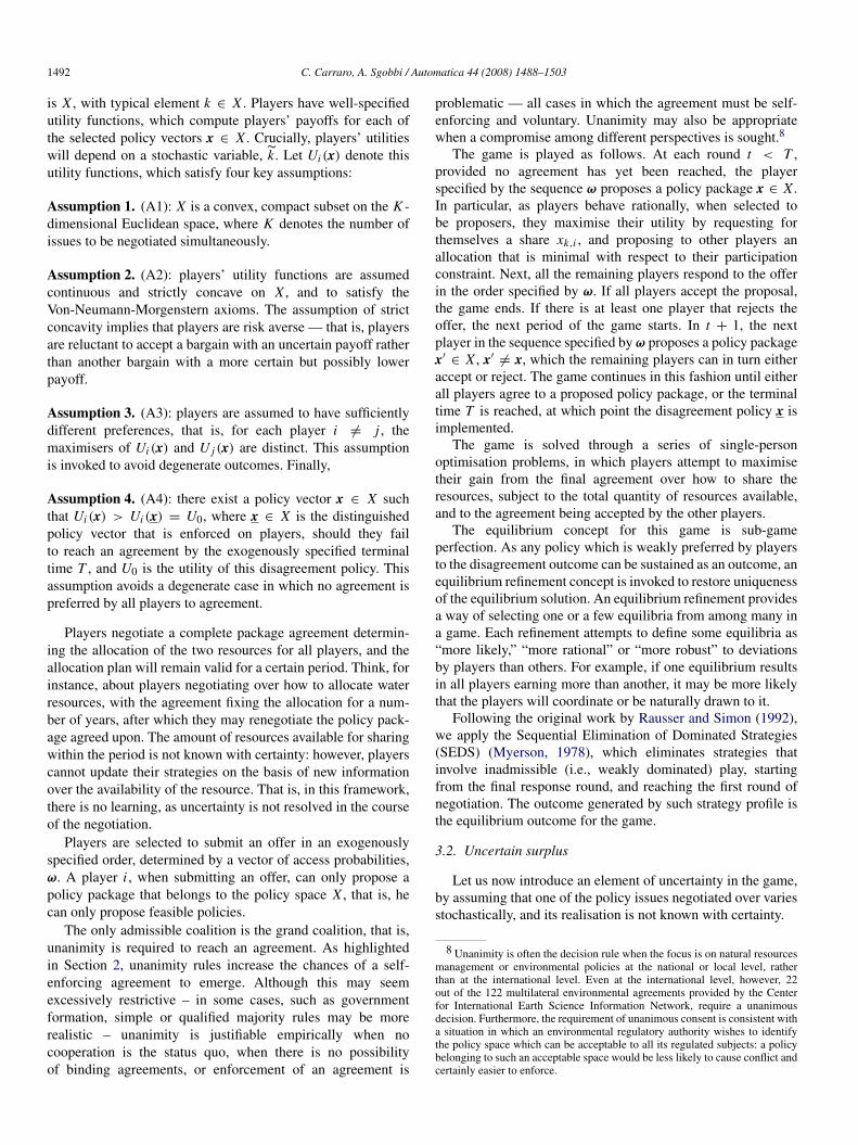
Table 3Sensitivity analysis – changing bargaining power

Player (i) ωiInitial location Perturbed location

A 0.2 0.1B 0.2 0.3C 0.2 0.2D 0.2 0.2E 0.2 0.2

Fig. 3. Expected utility constraints in round T − 1 — the effect of shiftingbargaining power.

role in shaping the equilibrium outcome. First, let us analysethe role of players’ relative bargaining power. To analyse it,we perform a second round of simulations which are identicalto the baseline case, with the exception of players’ bargainingpower. In particular, we assume that bargaining power shiftsfrom player A to player B, keeping the power of other playersconstant, as shown in Table 3.

Intuitively, one would expect that, while the player with ahigher access probability increases his equilibrium utility level,the other players experience a reduction in utility. The effectof increasing a player’s bargaining power is to tighten theconstraint the other players face when proposing an allocation,as shown in Fig. 3, where the participation constraint for playerB is higher in the case where bargaining power is shifted than inthe baseline case. Similarly, the effects of increasing a players’bargaining power is to relax the participation constraintsof player A in the penultimate round of negotiation, whileleaving the other players’ participation constraints substantiallyunchanged. Thus, if the negotiations proceed to round T − 1,player B may be able to extract a larger surplus than in thebaseline case.

Consider Fig. 4. Each cluster of bars decomposes the changein players’ expected utilities, as access is shifted from player Ato player B – keeping other players’ bargaining power constant.In round T − 1, the utility that player A gains from his ownproposal in the perturbed situation – compared to the baselineutility – is lower: this is because the participation constraint ofplayer B on player A is binding in the penultimate round inthe baseline case (see Table 2): increasing the bargaining powerof player B will necessarily lead to a tighter expected utilityconstraints, thus forcing player A to make a proposal which isless favourable to himself than would otherwise be the case. At

Fig. 4. Change in utilities from shifting bargaining power — round T − 1.

Fig. 5. Changes in players’ participation constraints.

Table 4Distance between players’ ideal point

A B C D E

A 0 2.24 6.00 4.47 4.47B 2.24 0 8.06 5.00 5.00C 6.00 8.06 0 5.66 5.66D 4.47 5.00 5.66 0 0E 4.47 5.00 5.66 0.00 0.00

the same time, player B gains substantially, independently ofwho is proposing in the penultimate round of the negotiationprocess.

At equilibrium, the effects of shifting bargaining power fromone player to another, keeping the other constant, may not belinear. The implication is that the ultimate effect of shiftingbargaining power cannot be predicted, as this is not linearlyrelated to the final outcome of the negotiation, but criticallydepends on other constitutional factors — such as decisionrules, players’ preference parameters, the relative distance oftheir ideal points, so on and so forth. This is shown by theresults of our simulation: the final impact depends on thebargaining design. Fig. 5 shows the evolution of players’participation constraints as we move backward in the game— that is, the difference between players’ expected utilitiesbetween the baseline case and the perturbed case.

It is clear that, through various interacting forces, that thedisadvantage of player A decreases as we move along the game,while the advantage of player B decreases. The cause of thiseffect is to be found in the preference structure and utilities ofthe players: the distance between player A and player B’s idealpoints is relatively small, as compared to the other two players(see Table 4). Thus, in the longer run, player A is able to benefitfrom the increased bargaining power of player B.


Table 5Perturbed constraints on the negotiated variables

n = 1 n = 2

Xn Baseline 130 100Perturbed 130 80

Fig. 6. Changes in players’ utilities from restricting the issue space.

Let us now look at the impact of restricting the valuesthat the negotiated variables can take. If the predictions oftheoretical models are correct, we would expect to see thatplayers have a lower utility from negotiations, as the bargainingspace – and as a consequence the gains from trade – isrestricted. The new upper bounds for negotiated variables arepresented in Table 5.

Fig. 6 shows the changes in utility level for each playerwhen they are selected to be the proposers in the respectivenegotiation rounds — that is, it is the difference in utilitiesthey enjoy when proposing an agreement in the restricted andbaseline cases. It is clear that all players experience a decreasein utility as compared with the baseline case. The decreasedoes not, however, uniformly affect all players: those who havestronger preferences for restricted policy issue (that is, thosewith a higher ideal point for X2, players A, B, and C) suffermore from this restriction than the other players. The decline inutility is mitigated by different weights that individual playersassign to X2 relative to X1, as indicated by different values ofηi,k in Table 1: thus, players A and B, who have a strongerpreference towards X2 as compared to X1, suffer a loss higherthan player C, who has a higher preferred point for X2, butassigns a low weights to this variable relative to the previoustwo players. This result of the simulation exercise is in line withboth theoretical findings of non-cooperative bargaining theoryand applications of non-cooperative bargaining models to waternegotiations (see Carraro, Marchiori, and Sgobbi (2005, 2007)).Furthermore, more iterations are needed before a limit pointequilibrium solution is found, indicating increased difficultiesin finding a compromise allocation.

Interestingly, players with a higher ideal point for therestricted issue will “bargain harder” in the last rounds ofthe negotiation game, and require a higher share of the totalresource available for themselves. This effect is shown in Fig. 7:should the final round of the negotiation game be reached,the first three players, when selected to be proposers, will askfor themselves a higher share of X2. The effect decreases forplayer C as the game proceeds backward, because of the largeropportunity that this player has to compensate for losses in X2

Table 6Changing the relative importance of the negotiated variables

Player D ηD,1 ηD,2

Initial 0.5 0.5Perturbed 0.2 0.8

Fig. 7. Change in players’ proposed shares — x2.

Fig. 8. Variation in player D proposals for x2.

with higher X1. These results are robust to further restriction inthe issue space.

Consider now the case in which one of the player’spreferences towards the two negotiated variables changes insuch a way that he now strongly prefers satisfying his idealquantity of one negotiated variable relative to the other.Intuitively, one would expect the equilibrium shares of thisplayer to change so that his equilibrium quantity of the stronglypreferred variable is higher than in the baseline simulationexercise.

In the simulation exercise, we change the relative weightsthat player D assigns to X2 relative to X1, as shown in Table 6.

As expected, player D will require a higher share of X2relative to the baseline case (see Fig. 8).

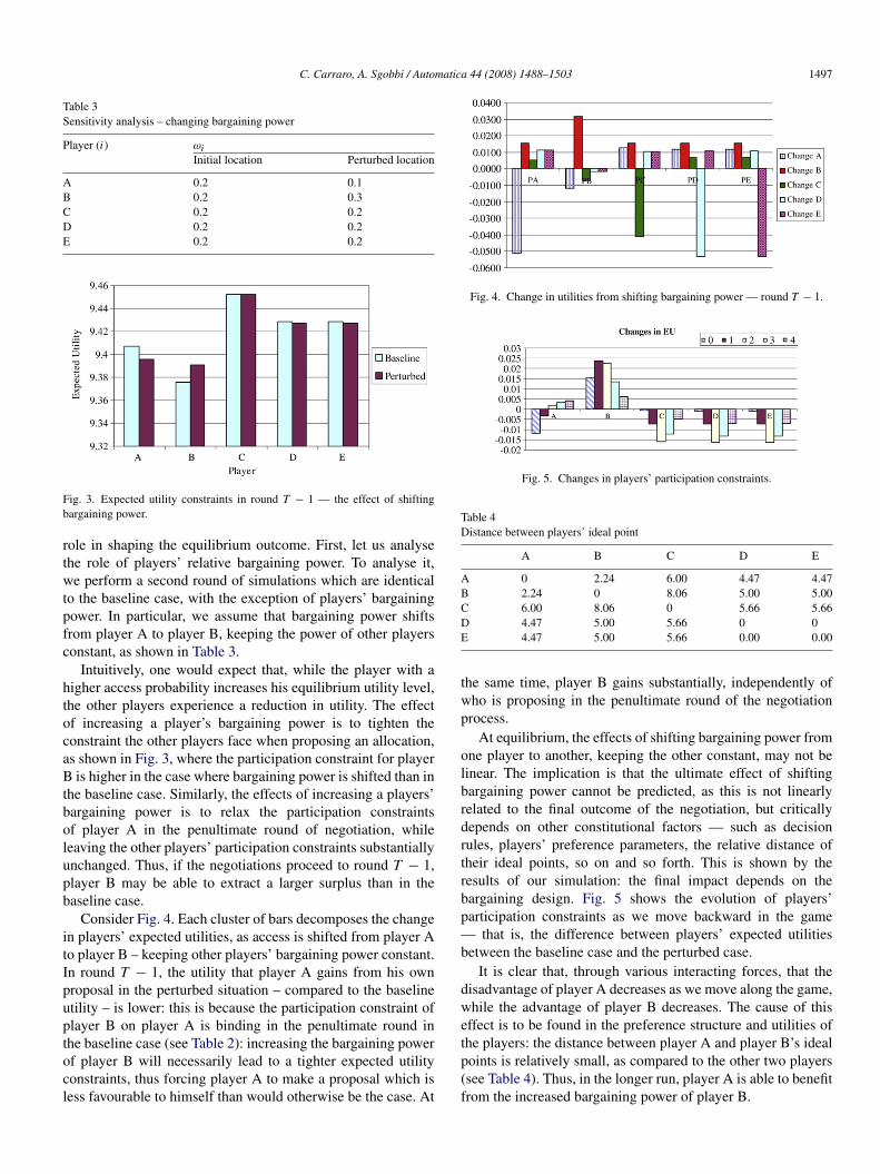
What is of interest is that his stronger position affords playerD a stronger bargaining position, and his participation con-straints in round T − 1 tightens, while the participation con-straints of the remaining players are substantially unchanged(Fig. 9, T −1). This effect is preserved through the backward in-duction process, and in equilibrium player D will enjoy a higherutility level (Fig. 9, Equilibrium). In this model, there seem tobe two sources of bargaining power: first of all, players’ access– which, however, is neither linearly nor monotonically relatedto players’ equilibrium payoffs – and players ideal points – bothin terms of their magnitude and relative importance.


dnuataduh

Fig. 9. Changes in players’ participation constraints in round T-1 and in equilibrium.

Finally, it is interesting to note that, in the long run, arelatively large change in players’ weighting of negotiatedvariables leads to utility levels that are significantly higher forthat player, but leaves the expected utilities of other playerssubstantially unchanged.

6. The role of uncertainty

One of the key aspects of negotiation processes isuncertainty over the size of the negotiated variables (the sizeof the pie). Let us analyse how this type of uncertainty affectsthe agreement and players’ utilities. In numerical analysis, welook at the impact of introducing a random component in theconstraint function for X2. The new constraint for this variablewill thus take the following form:∑

N

xi,2 ≤ X2 (6)

where X2 is an uncertain component of the size of the pie tobe divided. In the case of negotiations on water availability,for instance, the total quantity available depends in part onprecipitation levels, which, however, cannot be predicted withcertainty.

To demonstrate the relationship between the introductionof uncertainty in the realisation of one of the negotiatedvariables and the frequency of different solution, we reportthe results of a Monte Carlo experiment, in which we solvethe model for 100 randomly drawn values of X2, assumingan exogenously specified underlying probability distributionfor the unknown term. Using random inputs, the deterministicmodel is essentially turned into a random model.

The choice of the underlying distribution to simulate randomsampling may impact the results of the simulations. Forthe numerical example, we will assume that the randomcomponent of X2, X2, is drawn from a gamma probabilitydistribution,12 with shape parameter 13 and scale parameter 8.5.

12 There are various types of probability distribution one could use: the normalistribution is applicable to variables whose values are determined by an infiniteumber of independent random events; very rare events are best representedsing Poisson distribution. Normal distribution is symmetrical around the meannd, in general, it is used when (i) there is a strong tendency for the variable toake a central value; (ii) positive and negative deviations from the central valuere equally likely; and (iii) the frequency of deviations falls off rapidly as theeviations become larger. Gamma distribution is, on the other hand, widelysed in engineering to model continuous variables that are always positive andave a skewed distribution.

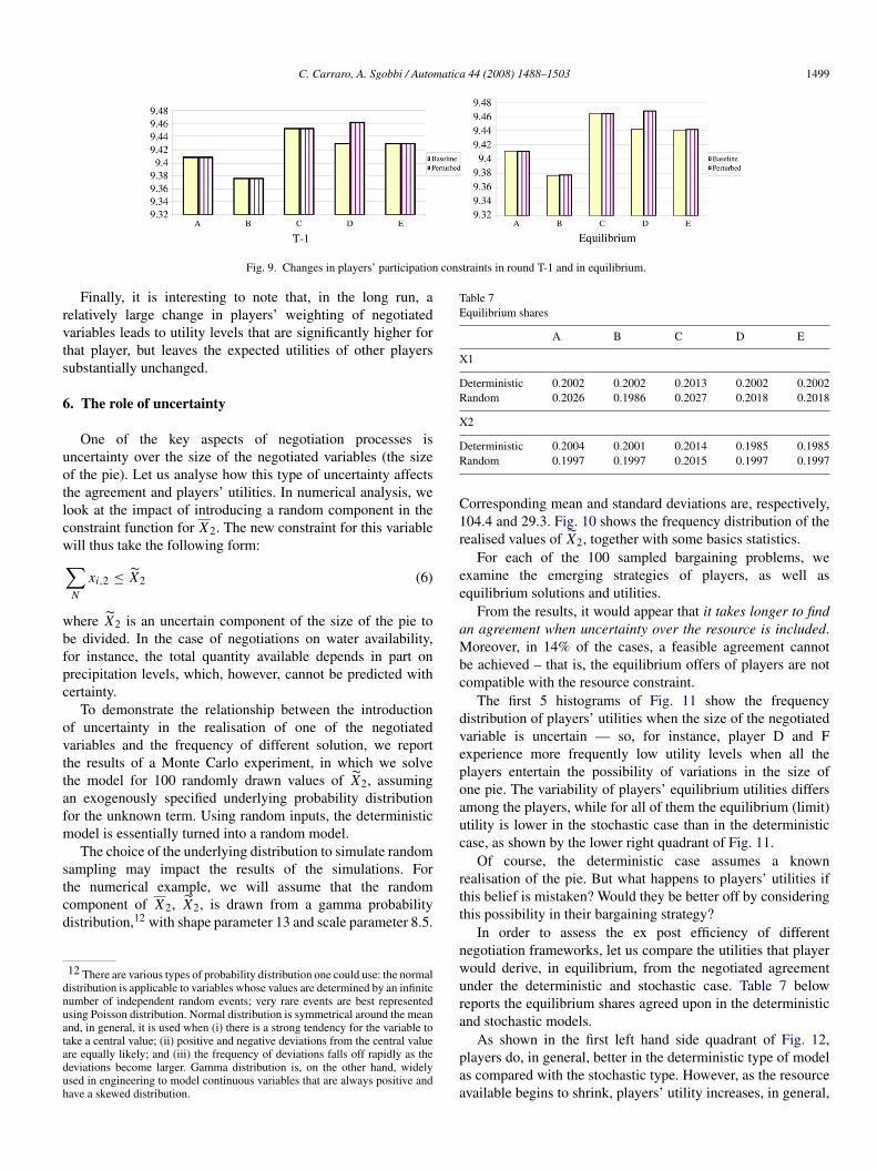
Table 7Equilibrium shares

A B C D E

X1

Deterministic 0.2002 0.2002 0.2013 0.2002 0.2002Random 0.2026 0.1986 0.2027 0.2018 0.2018

X2

Deterministic 0.2004 0.2001 0.2014 0.1985 0.1985Random 0.1997 0.1997 0.2015 0.1997 0.1997

Corresponding mean and standard deviations are, respectively,104.4 and 29.3. Fig. 10 shows the frequency distribution of therealised values of X2, together with some basics statistics.

For each of the 100 sampled bargaining problems, weexamine the emerging strategies of players, as well asequilibrium solutions and utilities.

From the results, it would appear that it takes longer to findan agreement when uncertainty over the resource is included.Moreover, in 14% of the cases, a feasible agreement cannotbe achieved – that is, the equilibrium offers of players are notcompatible with the resource constraint.

The first 5 histograms of Fig. 11 show the frequencydistribution of players’ utilities when the size of the negotiatedvariable is uncertain — so, for instance, player D and Fexperience more frequently low utility levels when all theplayers entertain the possibility of variations in the size ofone pie. The variability of players’ equilibrium utilities differsamong the players, while for all of them the equilibrium (limit)utility is lower in the stochastic case than in the deterministiccase, as shown by the lower right quadrant of Fig. 11.

Of course, the deterministic case assumes a knownrealisation of the pie. But what happens to players’ utilities ifthis belief is mistaken? Would they be better off by consideringthis possibility in their bargaining strategy?

In order to assess the ex post efficiency of differentnegotiation frameworks, let us compare the utilities that playerwould derive, in equilibrium, from the negotiated agreementunder the deterministic and stochastic case. Table 7 belowreports the equilibrium shares agreed upon in the deterministicand stochastic models.

As shown in the first left hand side quadrant of Fig. 12,players do, in general, better in the deterministic type of modelas compared with the stochastic type. However, as the resourceavailable begins to shrink, players’ utility increases, in general,


ac

Fig. 10. Distribution of X2.

Fig. 11. Frequency distribution of players’ equilibrium utilities.

when they take into account the uncertainty surrounding therealisation of the surplus. The explanation is intuitive: asplayers begin to account for uncertainty in their strategy, theywill try to negotiate harder, expecting a higher share of thesurplus, in order to increase their chance of coming closer totheir ideal.13

7. Relevance of the model for environmental and naturalresource management

The model proposed in this paper reproduces the negotiationprocess among multiple players who have to decide on how toshare a surplus of fixed (although uncertain) size. Negotiationsare approximated by an offer and counteroffer process. Theequilibrium outcome of negotiations is computed both in adeterministic setting and in the case in which uncertainty isaccounted for. Therefore, the modelling framework presented

13 Note that, because of the construction of our preference function, an excessllocation is a punishment for players. This may not be realistic in someircumstances.

in the previous sections can be an important tool to identifyunder what conditions negotiations on environmental andnatural resource management can actually achieve a consensusoutcome.

Natural resource and environmental management problemsare often complex, they interest several parties at the same time,and are characterised by different, often conflicting, objectives.One of the responses to improve their management in recentyears has been to promote collective negotiated decision-making procedures, both at the national and at the internationallevel. In real-life, there are many examples of international andnational negotiations over global and regional natural resources,such as the atmosphere, the seas, biodiversity, fish stocks, so onand so forth (for some examples, see for instance Breslin, Dolin,and Susskind (1992) and Breslin, Siskind, and Susskin (1990)).Through negotiations, proposals are put forward by interestedparties, who have both common and conflicting interests(Churchman, 1995), with the idea that negotiated decisionscan lead to management choices which are better adapted tolocal conditions, and can result in easier implementation, lesslitigation and improved stability of agreements.


is

Fig. 12. Changes in players’ equilibrium utility — deterministic vs. stochastic.

The model proposed in this paper can be fruitfully usedto explore natural resources and environmental managementproblems, by viewing negotiated decision making as amultiparty decision making activity: through strategies andmovements, actors (players) try to achieve an agreement whichis acceptable to all parties, and maximise their own satisfaction.The process of negotiating thus entails the presentation ofproposals and compromises, as well as players’ attempts toelicit opponents’ preferences and strategies. As such, themodel can be seen as an applied simulation tool whichcan be used by decision makers as a ‘negotiation-support-tool’. More formally, analytical models of negotiation allowapproaching the issue as a multi-variable decision makingprocess, whereby significant gains from bargaining can becreated by simultaneous negotiation over different aspects ofthe environmental problem. In addition, negotiated agreementsare likely to be more robust and easier to enforce, bothnationally and internationally.

The value added of exploring environmental managementproblems within a non-cooperative bargaining framework liesin the ability of the approach to help finding politically andsocially acceptable compromise. Our model can thereforebe helpful in exploring conflicts and opportunities in themanagement of natural resources which are shared amongdifferent users, for example at the national level, where there isa regulatory body which can impose a solution and enforce it,and thus the threat of enforcing a policy which is not negotiatedamong players is real.14 In addition, given that the equilibriumrequires the consensus of all negotiating parties, our model

14 As discussed below, application of our bargaining framework tonternational environmental problems can also be envisaged when there is aupranational environmental authority, e.g. at the EU level.

is consistent with a situation in which a regulatory authoritywishes to identify the policy space which can be acceptableto all its regulated subjects: a policy belonging to such anacceptable space would be less likely to cause conflict andcertainly easier to enforce.

The proposed model can find several applications, inparticular in the field of national or local natural resourcemanagement – where conflicts over how to share a resourceof a finite size are increasing. In fact, similar models havebeen used in the past to explore water allocation and pricingpolicies (Adams et al., 1996; Simon et al., 2003, 2006; Thoyeret al., 2001). So, for instance, the model can be used bya River Basin Authority wishing to implement bottom-upplanning approaches, thus allowing water users the possibilityto design, among themselves, a water allocation plan which canbe embraced by the authority. To do this, water users wouldbe required to define a proposal which is agreed upon amongall actors and respects environmental constraints. Furthermore,they would need to conclude their negotiation within a fixedperiod of time, after which the Authority would impose adefault water allocation plan. It is interesting to highlight that,in this context, the assumption of complete information maynot be too unrealistic: water users, for instance, are likely toknow the requirements and preferences of the other users with asufficient degree of precision. However, the amount of water tobe allocated is often uncertain (being subject to unpredictablefuture climatic events, for example). Therefore, the extensionof the model presented in this paper is crucially relevant forapplications to natural resource management.

Other applications in the field of natural resourcesmanagement can also be envisaged. Our non-cooperativebargaining approach can be useful to explore individuals’decisions and strategic incentives in the case of managing


common pool resources, in particular whenever a naturalresource is rival in consumption but limitation of access andpolicy enforcement can be difficult. A similar frameworkhas been used by Pinto and Harrison (2003) to modeltrade negotiation over environmental policies to abate carbondioxide, even though in their context the implications of severaldecision rules are explored, including unanimity. In the fieldof climate change, one could envisage an application of ourmodel to endogenise climate policy burden sharing rules –whereby players participating in an agreement negotiate overhow to share emissions’ allowances first, and then optimisetheir strategies, given the (negotiated) emission constraints.In the case of the European Union, for instance, the modelcould be used to explore the implications of bargaining forthe allocation of allowances under the EU Emission TradingScheme. Bargaining can take place among different EUcountries, and/or among firms inside each country. Uncertaintymay concern the global target to be achieved in the future (thatdepends on decision taken at the UNFCCC level). Unanimity isthe present decision rule at the EU level (and at least for somemore years) and the Commission has the power to sanctioncountries with which no agreement is reached (see Ellerman,Buchner, and Carraro (2007) for a description of the allocationprocess in the EU).

The non-cooperative multilateral, multiple issues bargainingmodel proposed in this paper could also be fruitfully appliedto exploring strategic incentives for more general tradenegotiations, such as WTO rounds on agricultural subsidies.

8. Conclusions

In this paper, we have proposed a new non-cooperativemultilateral bargaining model under uncertainty. In this model,players negotiate over multiple issues, i.e. players have payofffunctions that depend on the share of the surplus that theycan secure for themselves – with different negotiated variableshaving different importance for each player, thus generatingspace for tradeoffs among them. Furthermore, players havevarying access probabilities, which signal the relative strengthat the bargaining table and thus influence the equilibriumagreement. Uncertainty over the size of the total benefit thatplayers can achieve is also included in the model.

After having presented the model and its formal properties,through a series of numerical experiments in which fiveplayers negotiate over the respective share of two cakes, wehave examined the emerging equilibrium agreements and theircharacteristics. Let us summarise the main conclusions of ouranalysis.

First of all, when there is no uncertainty over negotiatedvariables, results are consistent with previous analyses andconform to expectations. As in the Rausser-Simon model andits applications, increasing the access probability of a playerwill yield outcomes that are more favourable to the “morepowerful” player, but also to players with similar preferredpositions. Convergence of the solution is attained in fewiterations of the model – which can in part address some of the

critiques moved to backward induction, as there is scepticismabout long and involved inductive chains.

This latter result no longer holds when we restrictsignificantly the range of admissible values for negotiatedvariables. Restricting the size that negotiated variables cantake reduces indeed the opportunities for trade, thus yieldingpotentially lower utilities to all players. In some cases,excessively reducing the boundaries of negotiated variablesmay shrink the bargaining space so much that no zone ofagreement remains. Should this result emerge when exploringa real problem using this framework, it would be advisableto attempt changing the decision rule – from unanimity toqualified majority, for instance. In such a manner, the rangeof admissible proposals may be increased – but the emergingagreement may no longer be efficient. Furthermore, there is noguarantee that, under decision rules other than unanimity and astochastic resource, a unique equilibrium still exists.

Importantly, the effect of bargaining power on theequilibrium agreement is non linear, and evolves in a complexway through the process of backward induction. The effectof shifting access depends crucially on other constitutionalfactors with which it interacts – such as decision rules, players’preference parameters, the relative distance of their ideal points,so on and so forth. Thus, there are synergies among players orissues that affect the ultimate impact of bargaining, contrary tothe assumptions of standard Nash games.

Finally, the paper focused on the role of uncertainty overone of the negotiated variables (the size of the total benefitthat players can achieve). We showed that uncertainty cruciallyaffects the equilibrium outcome and the players’ strategies. Inparticular:

(i) when uncertainty is introduced, the negotiation takes, onaverage, longer (14 rounds as opposed to 7 rounds in thedeterministic case);

(ii) in some cases, players’ strategies do not even converge toa feasible solution – that is, players’ offers crystallise onvalues that are not compatible with the resource constraintfor variables;

(iii) explicitly accounting for uncertainty in the realisation ofthe surplus leads, under some circumstances, players tobargain harder: ex post, they are better off only whenthe realisation of the surplus is low, as compared to thedeterministic case.

These results are in line with intuition. They thereforelend support to the hypothesis that non-cooperative bargainingis a useful framework for exploring negotiation processesand players’ strategic behaviour. Applying non-cooperativebargaining theory can provide some useful insights, based onformal models, as to which factors influence to a significantextent players’ strategies and, as a consequence, the resultingequilibrium agreement policy.

The modelling framework proposed in this paper isparticularly relevant for environmental applications. Negotiatedmanagement of natural resources, when several agents and/orinstitutions share the use of their resources and/or take decisionsthat can affect the availability of a common resource, can be


improved by using our bargaining model under uncertainty.Interesting applications of the deterministic version of themodel to water management can be found for example in Simonet al. (2006). The stochastic version is instead used by Sgobbiand Carraro (2007) to analyse a complex water managementproblem in northern Italy.

Acknowledgements

The authors are grateful two anonymous referees andto Ariel Dinar, Fioravante Patrone and above all CarmenMarchiori for helpful comments and remarks. All remainingerrors are obviously ours.

References

Adams, G., Rausser, G., & Simon, L. (1996). Modelling multilateralnegotiations: An application to California Water Policy. Journal ofEconomic Behaviour and Organization, 30, 97–111.

Alesina, A., Angeloni, I., & Etro, F. (2001). The political economy of unions,NBER working paper.

Bac, M., & Raff, H. (1996). Issue-by-issue negotiations: The role of informationand time preferences. Games and Economic Behavior, 13, 125–134.

Busch, L.A., & Horstmann, I. (1997). Signaling via agenda in multi-issuebargaining with incomplete information. Mimeo.

Breslin, J. W., Dolin, E. J., & Susskind, L. F. (1992). Internationalenvironmental treaty making. Cambridge, MA: Harvard Law School.

Breslin, J. W., Siskind, E., & Susskin, L. (1990). Nine case studies ininternational environmental negotiation. Cambridge, MA: Harvard LawSchool.

Carraro, C., Marchiori, C., & Sgobbi, A. (2005). World bank policy researchworking series: Vol. 3641. Applications of Negotiation theory to waterissues. The World Bank.

Carraro, C., Marchiori, C., & Sgobbi, A. (2007). Negotiating on water. Insightsfrom non-cooperative bargaining theory. Environment and DevelopmentEconomics, 12(2), 329–349.

Carraro, C., & Siniscalco, D. (1997). R&D cooperation and the stability ofinternational environmental agreements. In C. Carraro (Ed.), Internationalenvironmental negotiations: Strategic policy issues. Cheltenham: E. Elgar.

Cesar, H., & De Zeeuw, A. (1996). Issue linkage in global environmentalproblems. In A. Xepapadeas (Ed.), Economic policy for the environmentand natural resources. Cheltenham: E. Elgar.

Chae, S., & Yang, A. (1988). The unique perfect equilibrium of an N-personbargaining game. Economic Letters, 28, 221–223.

Chae, S., & Yang, A. (1994). A N-person pure bargaining game. Journal ofEconomic Theory, 62, 86–102.

Churchman, D. (1995). Negotiation: process, tactics, theory. Lanham, MD:University Press of America, Inc.

Diermeier, D., Eraslan, H., & Merlo, A. (2004). Bicameralism and governmentformation. In CTN 9th workshop 04.

Ellerman, A. D., Buchner, B., & Carraro, C. (2007). Allocations in theEuropean emissions trading scheme. Rights, rents and fairness. Cambridge:Cambridge University Press.

Eraslan, H., & Merlo, A. (2002). Majority rule in a stochastic model ofbargaining. Journal of Economic Theory, 103, 31–48.

Fatima, S., Wooldrige, M., & Jennings, N.R. (2003). Optimal agendas for multi-issue negotiation. Mimeo. University of Southampton.

Fershtman, C. (1990). The importance of agenda in bargaining. Games andEconomic Behavior, 2, 224–238.

Folmer, H., van Mouche, P., & Ragland, S. E. (1993). Interconnectedgames and international environmental problems. Environmental ResourceEconomics, 3, 313–335.

Gneezy, U., Haruvy, E., & Roth, A. E. (2003). Bargaining under adeadline: evidence from the reverse ultimatum game. Games and EconomicBehaviour, 45, 347–368.

Herrero, M. (1985). A strategic theory of market institutions. London: LondonSchool of Economics.

In, Y., & Serrano, R. (2003). Agenda restrictions in multi-issue bargaining (II):unrestricted agendas. Economics Letters, 79, 325–331.

Inderst, R. (2000). Multi-issue bargaining with endogenous agenda. Games andEconomic Behavior, 30, 64–82.

Jun, B.H. (1987). A structural consideration on 3-person bargaining.Department of Economics, University of Pennsylvania.

Krishna, V., & Serrano, R. (1996). A model of multilateral bargaining. Reviewof Economic Studies, 63, 61–80.

Kultti, K., & Vartiainen, H. (2004). A non-cooperative solution to thebargaining problem. Working paper.

Ma, C., & Manove, M. (1993). Bargaining with deadlines and imperfect playercontrol. Econometrica, 61, 1313–1339.

Manzini, P., & Mariotti, M. (2003). A bargaining model of voluntary environ-mental agreements. Journal of Public Economics, 87(12), 2725–2736.

Manzini, P., & Mariotti, M. (2005). Alliances and negotiations. Journal ofEconomic Theory, 121(1), 128–141.

McCarl, B. A. (2004). GAMS user guide: 2004. Version 21.3. GAMSDevelopment Corporation.

Merlo, A. (1997). Bargaining over government formation in a stochasticenvironment. Journal of Political Economy, 105, 101–131.

Merlo, A., & Wilson, C. (1995). A stochastic model of sequential bargainingwith complete information. Econometrica, 63, 371–399.

Myerson, R. B. (1978). Refinements of the Nash equilibrium concept.International Journal of Game Theory, 15, 133–154.

Pinto, L. M., & Harrison, G. W. (2003). Multilateral negotiations over climatechange policy. Journal of Policy Modeling, 25, 911–930.

Rausser, G., & Simon, L. (1992). A non cooperative model of collectivedecision making: a multilateral bargaining approach. Department ofAgricultural and Resource Economics, University of California, Berkeley.

Rubinstein, A. (1982). Perfect equilibrium in a bargaining model. Economet-rica, 50, 97–110.

Rusinowska, A., de Swart, H., & van der Rijt, J. W. (2005). A new model ofcoalition formation. Social Choice and Welfare, 24, 129–154.

Sgobbi, A., & Carraro, C. (2007). A stochastic multiple players multi-issuesnegotiation model for the piave river basin. Mimeo. Fondazione Eni EnricoMattei.

Shaked, A. (1986). A three-person unanimity game. Mimeo.Simon, L., Goodhue, R., Rausser, G., Thoyer, S., Morardet, S., & Rio, P. (2003).

Structure and power in multilateral negotiations: An application to FrenchWater Policy, edited.

Simon, L., Goodhue, R., Rausser, G., Thoyer, S., Morardet, S., & Rio, P.(2006). Structure and power in multilateral negotiations: an applicationto French water policy, In Paper presented at 6th Meeting of Game Theoryand Practice, 2006.

Stahl, I. (1972). Bargaining theory. Stockholm School of Economics.Thoyer, S., Morardet, S., Rio, P., Simon, L., Goodhue, R., & Rausser, G.

(2001). A bargaining model to simulate negotiations between water users.Journal of Artificial Societies and Social Simulation, 4.

Carlo Carraro holds a Ph.D. from PrincetonUniversity and is currently Chairman of the Departmentof Economics and Professor of Econometrics andEnvironmental Economics at the University of Venice.He is Director of Research of the Fondazione ENIEnrico Mattei and Research Fellow of CEPS, CEPRand CESifo. He is also Director of the Climate Impactsand Policy Division of the EuroMediterranean Centeron Climate Change (CMCC) and belongs to theScientific Advisory Board of the Potsdam Institute for

Climate, of the Research Network on Sustainable Development, Paris, and tothe High-Level Network of Environmental Economists set up by the EuropeanEnvironmental Agency.

Alessandra Sgobbi holds a Ph.D. in Analysisand Governance of Sustainable Development fromthe School of Advanced Studies of the Universityof Venice (Italy). Her main research interests arethe integration of “hard” and “soft” sciences inmodelling the economy-environment system, and theanalysis of negotiation processes through formal, gametheoretic models. She is collaborating with FEEM onvarious EU funded projects in the Natural ResourcesManagement and Climate Change Modelling and

Policy Programmes. Previously, she worked as a senior economist in theMinistry of Finance, Planning and Economic Development of the Republic ofUganda.

modelling negotiated decision making in environmental and natural resource management: a...

Documents