modelling of a bi-axial vibration energy harvester · the mechanical oscilla tions of the...
TRANSCRIPT
UNCLASSIFIED
Modelling of a Bi-axial Vibration Energy Harvester
Luke A. Vandewater and Scott D. Moss
Air Vehicles Division Defence Science and Technology Organisation
DSTO-TN-1174
ABSTRACT This report fully details the techniques involved in the modelling of a nonlinear and bi-axial vibration energy harvesting device. The device utilises a wire-coil electromagnetic (EM) transducer within a nonlinear oscillator created with a permanent-magnet/ball-bearing arrangement. The mechanical oscillations of the ball-bearing in response to bi-axial vibrations in a host structure induce a voltage across the coil, and therefore energy to power an attached device - such as an in-situ structural health monitoring system on an aircraft platform. Modelling of the mechanical dynamics and the electromechanical transduction of the harvester is undertaken by: means of finite element analysis (FEA), the homotopy analysis method (HAM), a novel probability-of-existence approach to vibro-impact, and numeric EM calculations. The models produced demonstrate high accuracy in comparison to a laboratory prototype.
RELEASE LIMITATION
Approved for public release.
UNCLASSIFIED
UNCLASSIFIED
UNCLASSIFIED
Published by Air Vehicles Division DSTO Defence Science and Technology Organisation 506 Lorimer St Fishermans Bend, Victoria 3207 Australia Telephone: 1300 DEFENCE Fax: (03) 9626 7999 © Commonwealth of Australia 2013 AR-015-598 May 2013
APPROVED FOR PUBLIC RELEASE
UNCLASSIFIED
UNCLASSIFIED
Modelling of a Bi-axial Vibration Energy Harvester
Executive Summary Continuing developments in the Structural Health Monitoring (SHM) domain hold great promise for the application of in-situ devices on air platforms, enabling the Australian Defence Force (ADF) to move from the current expensive time-based maintenance approach, to a more cost-effective condition-based approach. DSTO is investigating vibration energy harvesting (VEH) which is a foundation technology for powering many in-situ SHM applications (for example, autonomous SHM systems that are designed to be retro-fitted onto a vehicle to monitor structural and/or corrosion hotspots). While commercial VEH solutions are available, the environment specific to air platforms inhibit their use – that is, commercial devices are often heavy, respond to only uni-axial vibrations, do not operate well at high accelerations, and produce output power at a very narrow frequency bandwidth. Recent work at the DSTO has resulted in the development of a bi-axial VEH device, capable of harvesting useable energy from wide-band bi-axial excitations within a small device footprint, and therefore proving appropriate for integration into an in-situ SHM system for air platforms. The device operates as a permanent-magnet/ball-bearing mechanical oscillator, free to respond to host structure excitations. An electromagnetic wire coil transducer (between the magnet and ball-bearing) produces electrical output due to a changing magnetic field distribution as the ball-bearing oscillates. This Technical Note provides a brief summary on the functioning of the VEH device, and details the modelling work undertaken at the DSTO to investigate the device. The complex nonlinear dynamics and electromagnetic properties of the device require numerical computation tools such as finite element analysis (FEA), and advanced mathematical techniques pertaining to nonlinear oscillations and discontinuous systems. The outcome of the modelling work is a full description of the mechanical dynamics and electrical transduction of the VEH device, and a capability for optimisation work and guidance for design decisions.

UNCLASSIFIED DSTO-TN-1174
UNCLASSIFIED
UNCLASSIFIED DSTO-TN-1174
Authors
Luke Vandewater Air Vehicles Division Luke Vandewater is four years into completing the double degree of Bachelor of Engineering (Robotics and Mechatronics) and Bachelor of Science (Computer Science and Software Engineering) at Swinburne University. He undertook this work while on a one-year contract with DSTO Smart Structures and Advanced Diagnostic Group, where he investigated various vibration energy harvesting techniques.
____________________ ________________________________________________
Scott Moss Air Vehicles Division Dr. Scott Moss is currently a Senior Research Scientist within the Air Vehicles Division of the Australian Defence Science and Technology Organisation (DSTO). In 2003 he was awarded a DSTO Defence Science Fellowship and spent a year working in the UCLA Active Materials Laboratory investigating energy harvesting from aircraft structures. This work continues as an exploration of techniques for powering, and communicating with, structural health monitoring devices.
____________________ ________________________________________________
UNCLASSIFIED

UNCLASSIFIED DSTO-TN-1174
UNCLASSIFIED
UNCLASSIFIED DSTO-TN-1174
Contents
1. INTRODUCTION............................................................................................................... 1 1.1 Vibration energy harvesting ................................................................................... 1 1.2 Prototype harvester................................................................................................... 1
2. MODELLING....................................................................................................................... 2 2.1 Three dimensional COMSOL modelling............................................................. 2 2.2 Mechanical dynamics............................................................................................... 4
2.2.1 An equation of motion for the unrestrained ball-bearing ................. 4 2.2.1.1 The homotopy analysis method solution............................................. 5 2.2.2 Vibro-impact operation and the probability-of-existence ................. 7 2.2.2.1 Parallelised computation of system states ........................................... 9
2.3 Electromagnetic transduction ............................................................................... 10 2.3.1 Coil modelling and matched resistive load power generation....... 10 2.3.1.1 Numerical computation of power output.......................................... 11
3. CONCLUSION .................................................................................................................. 13
4. REFERENCES .................................................................................................................... 13
APPENDIX A: THREE DIMENSIONAL COMSOL MODELS .................................. 17 A.1. Static model (magnetic fields, no currents)............................... 17
A.1.1 Parameters ........................................................................ 17 A.1.2 Geometry........................................................................... 17 A.1.3 Physics implementation.................................................. 18 A.1.4 Solver configuration ........................................................ 19
A.2. Transient model (magnetic fields, deformed geometry, global ODEs) ................................................................................... 19 A.2.1 Parameters ........................................................................ 19 A.2.2 Geometry........................................................................... 20 A.2.3 Physics implementation.................................................. 21 A.2.4 Solver configuration ........................................................ 23
APPENDIX B: HARVESTER BALL-BEARING DYNAMICS .................................... 25 B.1. Homotopy analysis method ......................................................... 25
APPENDIX C: VIBRO-IMPACT DYNAMICS .............................................................. 28 C.1. Event-driven Mathematica numeric solve script...................... 28
C.1.1 Input (ImpactDemo.nb) .................................................. 28 C.1.2 Output ............................................................................... 29
C.2. Calculation parallelisation script ................................................ 29
UNCLASSIFIED

UNCLASSIFIED DSTO-TN-1174
UNCLASSIFIED
C.2.1 Input (ParallelImpactScript.nb) ..................................... 29 C.2.2 Output ............................................................................... 31 C.2.3 Computation comparison............................................... 32
APPENDIX D: ELECTROMAGNETIC TRANSDUCTION ........................................ 33 D.1. Model data extraction in MATLAB
(modelExporter_main.m) .............................................................. 33 D.2. Numeric coil output Mathematica script ................................... 35
D.2.1 Input (InducedVoltage.nb) ............................................. 35 D.2.2 Output ............................................................................... 38

UNCLASSIFIED DSTO-TN-1174
1. Introduction
1.1 Vibration energy harvesting
Vibration energy harvesting has attracted a large amount of attention from the scientific community in recent years [1,2], and in particular is being investigated at DSTO for the purposes of powering in-situ structural health monitoring systems [3,4]. Many current commercial designs are not suitable for use in the aerospace domain, as they are often large [5], respond only uni-axially [6], and to a narrow bandwidth of excitation frequencies [7]. In the interests of an in-situ device, DSTO is investigating a compact harvester design intended to produce output power from large host accelerations and a wide-band of frequencies [8]. Nonlinear vibration energy harvesting approaches have shown promise for these requirements, for example vibro-impact [9], bi-stability [10], and buckling [11] etc, all used to increase device bandwidth. In addition, varying transducer technologies (electromagnetic [12,13], magnetoelectric [4], etc) have allowed compact designs. Vibration energy harvesting techniques developed by DSTO are analysed in this Technical Note, in particular the investigation of a prototype harvesting arrangement (utilising a permanent-magnet/ball-bearing mechanical oscillator, and an electromagnetic transducer). A brief background is provided on the harvesting work, with an emphasis on the description of the modelling undertaken to explore the prototype harvester. The main purpose of this Technical Note is to provide sufficient technical detail so as to allow the modelling work described herein to be reproduced. To facilitate this goal a comprehensive set of appendices has been included, and a companion Compact-Disk is attached containing modelling code and other files. 1.2 Prototype harvester
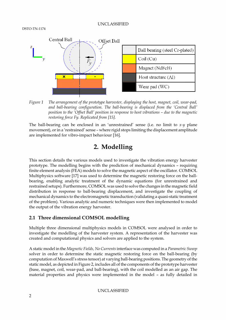
The vibration energy harvester prototype being developed at DSTO [3] (represented schematically in Figure 1) consists of wire-coil electromagnetic (EM) transducer located between a permanent magnet and a ball-bearing. The magnet/ball-bearing acts as a mechanical oscillator, producing relative motion in response to host structure vibrations. The ball-bearing moves in the x-y plane across the surface of a wear-pad on top of the transducer, subject to a magnetic restoring force. The motion of the ball-bearing across the magnet produces a change in the magnetic field distribution in the volume occupied by the EM transducer, resulting in an induced electromotive force (EMF) in the wire-coil by Faraday’s Law of Induction [14], and hence power output across an electrical load.
UNCLASSIFIED 1
UNCLASSIFIED DSTO-TN-1174
Figure 1 The arrangement of the prototype harvester, displaying the host, magnet, coil, wear-pad,
and ball-bearing configuration. The ball-bearing is displaced from the ‘Central Ball’ position to the ‘Offset Ball’ position in response to host vibrations – due to the magnetic restoring force Fy. Replicated from [15].
The ball-bearing can be enclosed in an ‘unrestrained’ sense (i.e. no limit to x-y plane movement), or in a ‘restrained’ sense – where rigid stops limiting the displacement amplitude are implemented for vibro-impact behaviour [16].
2. Modelling
This section details the various models used to investigate the vibration energy harvester prototype. The modelling begins with the prediction of mechanical dynamics – requiring finite element analysis (FEA) models to solve the magnetic aspect of the oscillator. COMSOL Multiphysics software [17] was used to determine the magnetic restoring force on the ball-bearing, enabling analytic treatment of the dynamic equations (for unrestrained and restrained setups). Furthermore, COMSOL was used to solve the changes in the magnetic field distribution in response to ball-bearing displacement, and investigate the coupling of mechanical dynamics to the electromagnetic transduction (validating a quasi-static treatment of the problem). Various analytic and numeric techniques were then implemented to model the output of the vibration energy harvester. 2.1 Three dimensional COMSOL modelling
Multiple three dimensional multiphysics models in COMSOL were analysed in order to investigate the modelling of the harvester system. A representation of the harvester was created and computational physics and solvers are applied to the system. A static model in the Magnetic Fields, No Currents interface was computed in a Parametric Sweep solver in order to determine the static magnetic restoring force on the ball-bearing (by computation of Maxwell’s stress tensor) at varying ball-bearing positions. The geometry of the static model, as depicted in Figure 2, includes all of the components of the prototype harvester (base, magnet, coil, wear-pad, and ball-bearing), with the coil modelled as an air gap. The material properties and physics were implemented in the model – as fully detailed in
UNCLASSIFIED 2

UNCLASSIFIED DSTO-TN-1174
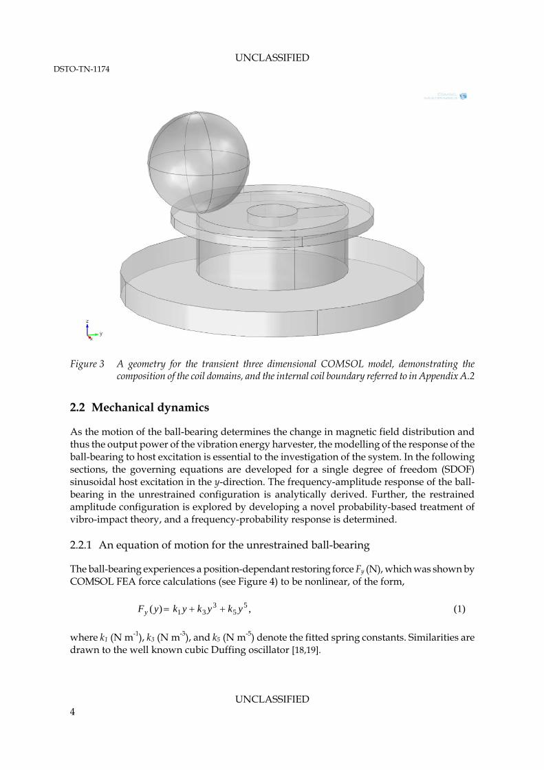
Appendix A.1. By solving in the parametric sweep, a position-dependant restoring force was determined for use in later analysis. The results show that the restoring force acts similar to a softening spring in a mass-spring-damper system. Refer to Appendix A.1 for details on the model setup – including the parameters, geometry, physics, and solver configurations required. A transient model requires the combination of the Magnetic Fields interface (for magnetic and electrical properties), the Deformed Geometry interface (to produce the ball-bearing movement in time), and the Global ODEs interface (to define a load attached to the coil). The complex coupling of these physics modes requires care in the setup of the model and solvers, all of which is detailed in Appendix A.2. The coil was handled in the model as an active component - a numerically calculated multi-turn coil domain, requiring a purpose-built geometry as in Figure 3. The movement of the ball-bearing was user-defined, as a sinusoidal function (matching the realistic displacement of the ball-bearing in response to a sinusoidal base displacement). The movement of the ball-bearing across the coil domain produces an induced voltage, and a current through a defined load. The results show that the system can be treated quasi-statically (that the static restoring force can be used dynamically, and the mechanical and transduction problems can be treated separately) - highlighted in particular in section 2.3.
Figure 2 A meshed geometry for the static three dimensional COMSOL model, demonstrating the
size of the mesh in various geometry components (domains)
UNCLASSIFIED 3
UNCLASSIFIED DSTO-TN-1174
Figure 3 A geometry for the transient three dimensional COMSOL model, demonstrating the
composition of the coil domains, and the internal coil boundary referred to in Appendix A.2
2.2 Mechanical dynamics
As the motion of the ball-bearing determines the change in magnetic field distribution and thus the output power of the vibration energy harvester, the modelling of the response of the ball-bearing to host excitation is essential to the investigation of the system. In the following sections, the governing equations are developed for a single degree of freedom (SDOF) sinusoidal host excitation in the y-direction. The frequency-amplitude response of the ball-bearing in the unrestrained configuration is analytically derived. Further, the restrained amplitude configuration is explored by developing a novel probability-based treatment of vibro-impact theory, and a frequency-probability response is determined. 2.2.1 An equation of motion for the unrestrained ball-bearing
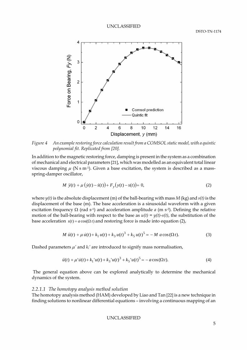
The ball-bearing experiences a position-dependant restoring force Fy (N), which was shown by COMSOL FEA force calculations (see Figure 4) to be nonlinear, of the form,
,)( 55
331 ykykykyFy (1)
where k1 (N m-1), k3 (N m-3), and k5 (N m-5) denote the fitted spring constants. Similarities are drawn to the well known cubic Duffing oscillator [18,19].
UNCLASSIFIED 4
UNCLASSIFIED DSTO-TN-1174
Figure 4 An example restoring force calculation result from a COMSOL static model, with a quintic
polynomial fit. Replicated from [20].
In addition to the magnetic restoring force, damping is present in the system as a combination of mechanical and electrical parameters [21], which was modelled as an equivalent total linear viscous damping (N s m-1). Given a base excitation, the system is described as a mass-spring-damper oscillator,
,0)()()()()( tstyFtstytyM y (2)
where y(t) is the absolute displacement (m) of the ball-bearing with mass M (kg) and s(t) is the displacement of the base (m). The base acceleration is a sinusoidal waveform with a given excitation frequency (rad s-1) and acceleration amplitude a (m s-2). Defining the relative motion of the ball-bearing with respect to the base as u(t) = y(t)-s(t), the substitution of the base acceleration )cos()( tats and restoring force is made into equation (2),
).(cos)()()()()( 55
331 taMtuktuktuktutuM (3)
Dashed parameters ’ and ki’ are introduced to signify mass normalisation,
).(cos)(')(')(')(')( 55
331 tatuktuktuktutu (4)
The general equation above can be explored analytically to determine the mechanical dynamics of the system. 2.2.1.1 The homotopy analysis method solution The homotopy analysis method (HAM) developed by Liao and Tan [22] is a new technique in finding solutions to nonlinear differential equations – involving a continuous mapping of an
UNCLASSIFIED 5
UNCLASSIFIED DSTO-TN-1174
assumed solution into a series solution. HAM was applied to the equation developed in section 2.2.1 in a similar fashion to previous results exploring a forced Duffing equation [23]. The HAM approach begins by defining two new variables for substitution,
,t (5)
)()( Atu , (6)
.)cos()(')('
)(')(')(5
553
33
12
akAkA
kAAA
(7)
The HAM approach produces series solutions to the new variables in equations (5) and (6) by means of solution deformations – dependant on the construction of a nonlinear operator from equation (7). Details of the HAM procedure with regard to nonlinear operators and solution deformations are left to Appendix B.1. The series solutions take the form,
,)()()(0
0
nn (8)
.1
0
nnAAA (9)
The form of the initial term in the )( series determines the form of the HAM solution, and is selected as the well-known harmonic balance method solution to the forced Duffing-type oscillator [19],
),cos()(0 (10)
where β is the unknown phase difference. The chosen initial term is referred to as the base function, and serves as an initial solution for the development of the homotopy. Continual solution deformations are developed from the base function and substituted into the series solutions, obtaining successively higher harmonics in the solution to equation (4). For example, the 1st order solution is,
33 0
0 2
5 55 0 5 0
2 2
'( ) cos cos3
32
5 ' 'cos3 cos5 ,
128 384
k Au t A t t
k A k At t
(11)
,'8
'5
4
'3' 22
022
2405
2032
1 aAAkAk
k
(12)
UNCLASSIFIED 6
UNCLASSIFIED DSTO-TN-1174
405
203
21 '5'6)'(8
'8)tan(
AkAkk
. (13)
The HAM approach clearly shows higher odd harmonics in the solution, admitting possible ‘superharmonics’. Convergence is controlled with selection of the auxiliary control parameter
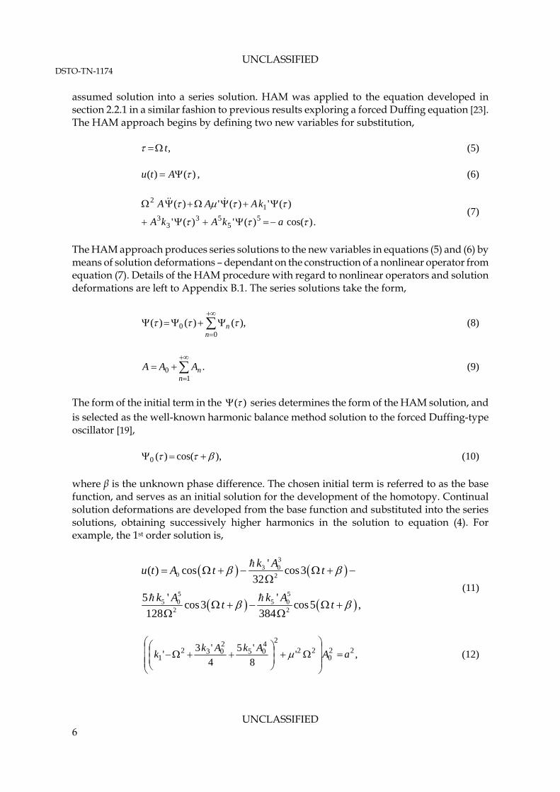
(as described by Liao and Tan [ 22]). The 1st order HAM solution represents an approximate analytic solution to the nonlinear differential equation (4), from which displacement predictions can be made (as in Figure 5).
Figure 5 A comparison between experimental displacements and the HAM model results. The ‘drop-
down’ frequency at higher drive forces are accurately modelled, and the frequency-displacement model matches well. Replicated from [20].
2.2.2 Vibro-impact operation and the probability-of-existence
The differential equation (4) derived in section 2.2.1 is now subjected to amplitude restraints to explore the vibro-impact operation of the harvester in the restrained configuration. Given that the oscillation of the ball-bearing is limited by a rigid stop located at (m) from the neutral position (as in Figure 6), impacts occur under certain conditions.
UNCLASSIFIED 7

UNCLASSIFIED DSTO-TN-1174
Figure 6 An example configuration for the restrained, vibro-impacting vibration energy harvester,
with rigid stops installed at gap Replicated from [24].
During the impact period, the contact mechanics are modelled by Hertzian contact theory, modified to include energy loss (hysteric damping) - the Hyster-Hertz contact model [25]. This model is derived under assumptions of non-conforming and small contact area collisions, with no plastic deformation and no friction between the objects. Previous work [26] derives the relative Hyster-Hertz contact force as,
))1()(
)(
4
31())(()())(),(( 22/3 e
tu
tutuKSgntutuF HZHC
, (14)
where e is the coefficient of restitution, and KHZ is the Hertzian contact stiffness determined from ball-bearing radius R1 (m) and material properties (Poisson’s Ratio and Young’s Modulus E),
)(3
4
21
1
hh
RK HZ
, (15)
UNCLASSIFIED 8
UNCLASSIFIED DSTO-TN-1174
i
ii E
h 21
. (16)
where i = 1, 2. The Hertzian contact stiffness is 8.70×10⁹ N m-3/2 for a steel ball-bearing (R1 = 12.7 mm, = 0.3, E1 = 200 GPa) on an aluminium stop (2= 0.33, E2 = 70 GPa) impact. Finally, the governing equations are formed,
)(tu :
),)((cos)(')(')(')()( 05
53
31 ttatuktuktuktutu
,)0()0( 00 uuuu (17) )(tu :
),)((cos
))1()(
4
31())()((
)(')(')(')()(
1
2
1
2/3
55
331
tta
eu
tutuSgnK
tuktuktuktutu
WWHZ
,)0()0( 11 uuuu W (18)
with initial conditions , , , , , and selected for continuity between equations. Mathematica software [27] was used to run simulations of the above system of equations, with an event-driven switching technique using ‘NDSolve’ functionality. Appendix
0t 0u 0u 1t 1u 1u
C.1 fully details the scripting developed. The result of a system simulation is that, at given initial conditions of displacement, velocity, and the phase difference between the base and ball-bearing, a system ‘state’ is determined. The behaviour of interest is continuous impacting (indicating high-energy output operation) - defined as the system state ‘Steady State Impacting’, and corresponding in the time series to sustained and consecutive impacts. Two other possible system states are ‘Transient Impacting’ (falling to a low energy operation mode after briefly impacting), and ‘Not Impacting’ (existing only in the low energy operation mode). Determining system states over all possible initial conditions, and over varying drive frequency values, a metric for vibro-impact regime existence is found (for more detail, refer to [24, 26]). The ratio of ‘Steady State Impacting’ states to all states is defined as the probability-of-existence, and displaying this as a function of frequency results in the frequency-probability response of a given system. 2.2.2.1 Parallelised computation of system states As discussed above, the system of equations of the vibro-impacting harvester need to be simulated over a large number of variables - initial conditions, drive parameters, rigid stop sizes, etc. Mathematica has inbuilt parallel processing functionality – allowing simulations to be distributed across multiple kernels and therefore computed simultaneously with multiple CPU cores. Due to overheads involved in the distribution process and the external data saving
UNCLASSIFIED 9

UNCLASSIFIED DSTO-TN-1174
mechanism implemented, a n-cores to n-times improvement is not achieved – however with heavily CPU/RAM intensive calculations such as looped ‘NDSolve’ calculations, improvement is significant. Using an 8-core machine (i7-920 @ 2.67 GHz, 16GB RAM), the average runtime of batch impact stitching simulations is decreased from 0.06 seconds per solution on one kernel, to 0.01 seconds per solution on 8 kernels – over a test run of 5,000 simulations. Similar performance was noted over full probability-of-existence solution sets requiring 250,000+ simulation loops. Appendix C.2 details scripting techniques enabling the parallelised execution of the script outlined in Appendix C.1. 2.3 Electromagnetic transduction
As described previously, the movement of the ball-bearing across the coil produces a change in magnetic flux through it, therefore inducing voltage by Faraday’s Law of Induction and hence power in an attached electrical load. Modelling for this electromagnetic transduction was undertaken by numerical analysis of finite element models created in COMSOL. A coupled transient mechanical and electromagnetic model was solved with Magnetic Fields and Deformed Geometry interfaces as discussed in section 2.1. This coupled transient model was used to determine the effect of the electrical load on the transduction, and on the mechanical dynamics. It was demonstrated that the back EMF from current flow in the circuit had no impact on the magnetic restoring force, and that the voltage across a resistive load is equal to that produced by voltage divider on the unloaded circuit (refer to [28] for full details). Or more simply, that the ball-bearing dynamics and transduction mechanism have negligible dynamic interaction. Therefore, the modelling is justified in separating the mechanical and electrical aspects of the problem. Combining the two separate physics models quasi-statically provides a representative time-varying output for the vibration energy harvester. 2.3.1 Coil modelling and matched resistive load power generation
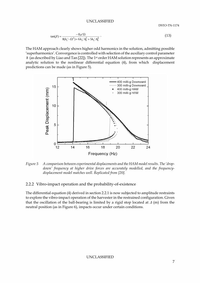
Given the assumptions of quasi-static behaviour, modelling the magnetic flux becomes a simple task for COMSOL. The static three-dimensional model detailed in section 2.1 was used to evaluate the B field (magnetic flux density) by enforcing flux conservation, as the ball is displaced in the x-y plane. COMSOL produced the B field at multiple interpolated points (x,y,z), which was then used in the following analysis to determine the output voltage by an implementation of Faraday’s Law of Induction. A coil was modelled in the analysis as discrete wire loops, arranged as a simple square packed array within given parameters of outer (rout) and inner radius (rin), and coil height (h). A coil turns ratio Nratio of 15.1~12/4 is used [28] to compare a square packed array to a realistic hexagonal packed wound wire-coil, shown in Figure 7.
UNCLASSIFIED 10
UNCLASSIFIED DSTO-TN-1174
Figure 7 A photo of a hexagonally packed wound wire coil transducer, with inner and outer radii of 5
and 15 mm respectively. Replicated from [28].
As resistance can be calculated from the coil geometry, matched resistive load voltage was found as a voltage divider from the unloaded calculation, and output power was calculated. The modelling approach here can be used with any displacement in the x-y plane (i.e. biaxial harvesting), and easily extended to multiple-coil arrangements (to harvest from circular motions). 2.3.1.1 Numerical computation of power output The voltage induced by the coil is a function of the magnetic flux through each wire loop of the coil, where the flux in each wire loop is defined as the surface integral of the B field component normal to the surface enclosed by the loop,
,1
N
i
iind dt
dV (19)
,),(
i iSx Syzi yxBdydx (20)
where Si is the surface enclosed by the i-th coil wire loop (normal to the z direction), Bz(x,y) is the discrete value of the z-direction component of the B field at an interpolated point (x,y) on the surface, and dx and dy are sufficiently small widths of interpolation. Combining equations (19) and (20), including the aforementioned coil turns ratio, and writing the B field as a
UNCLASSIFIED 11

UNCLASSIFIED DSTO-TN-1174
function of ball-bearing positions and , a final expression for determining the
induced voltage in a coil as a function of time is developed,
)(tux )(tu y
.))(),(,,()(1
N
i Sx Syyxzratioind
i i
tutuyxBdydxdt
dNtV (21)
The displacement modelling work of section 2.2 was used to determine the ball-bearing position with respect to time in the x-y plane. With respect to a resistive loaded harvester, the calculated induced voltage was applied to a simple coil/load voltage divider, and output voltage is determined. Figure 8 demonstrates the open-circuit output voltage as a function of frequency for a SDOF arrangement, compared to experimental measurements.
Figure 8 A comparison between the peak open circuit output voltage of a prototype energy harvester
as a function of frequency (for a frequency down-sweep), and the results of the numeric model of the prototype. For a 500 milli-g base excitation, at 16 Hz, the measured voltage is 0.489 V, and the predicted voltage is 0.462 V. Replicated from [28].
In addition, the peak power across a matched resistive load can be calculated as,
,)2/( 2
,
coil
pindp R
VP (22)
,2)( 1
2,
N
ii
cuwire
curatiocoil r
rNR
(23)
where Vind,p is the peak open circuit voltage (note that attaching a matched load resistor across the coil will halve the coils output voltage), Rcoil is the resistance of the coil, rwire,cu is the radius of the copper wire , ρcu is the resistivity of copper, and ri is the radius of the i-th wire loop. For
UNCLASSIFIED 12
UNCLASSIFIED DSTO-TN-1174
UNCLASSIFIED 13
4.0 Ω coil transducer) can en be estimated using equation 22, and is found to be 20.3 mW.
varyi determining the flux variation
a 12 Hz, 500 milli-g base excitation Figure 8 shows a maximum measured open circuit voltage of 0.571 V. The maximum output power of the prototype harvester (th Appendix D contains two example scripts – D.1 provides the extraction of data from COMSOL in MATLAB, and D.2 allows the data to be analysed in Mathematica. Assuming a radial symmetric flux distribution, a SDOF static COMSOL solve is rotated in the x-y plane, the coil flux computations are made for each ball-bearing position, and the resultant position-
ng flux is interpolated on the plane. Calculating the path of the ball-bearing )(tux and )(tu y in the plane and )(t produces the output ind(t)
nd peak power PP.
3. Conclusion
16 Hz, 500 milli-g excitation, comparing well with e predicted output voltage of 0.462 V.
4. References
S. Beeby, N. White, Energy harvesting for autonomous systems, Artech House, Boston, 2010.
S. Priya, D. J. Inman, Energy harvesting technologies, Springer, New York, 2009.
, Vibration energy conversion device, U.S. Patent Application, 13/464701, filed 4th ay 2012.
electric transduction, J. Int. Mat. Sys. Struct., doi: 10.1177/ 045389X12443598 (2012).
of energy harvesting sources for embedded systems,
voltage V
a
A prototype harvesting arrangement has been investigated with multiple analytical and numerical models, in order to fully understand the system and provide future design guidance and optimisation. The mechanical dynamics were modelled as a quintic-modified Duffing equation and solved by HAM, and the vibro-impact dynamics of the restrained configuration were described by a probability-of-existence approach. The transduction mechanism was numerically treated from FEA results in order to determine output characteristics. All involved COMSOL FEA models have been fully detailed, in terms of the setup requirements. Computational scripts have been detailed to demonstrate the modelling techniques, and the models appear to provide a predicted response which closely matches the response of the vibration energy harvester prototype investigated in the laboratory. The prototype examined used a 4.0 Ω coil transducer, and was experimentally shown to produce an open circuit voltage of 0.489 V from ath
1 2 3 S. D. MossM 4 S. D. Moss, J. E. McLeod, S. C. Galea, Wideband vibro-impacting vibration energy harvesting using magneto1 5 S. Chalasani, J. M. Conrad, A surveyIEEE Southeastcon, (2008) 442 – 447.
UNCLASSIFIED DSTO-TN-1174
S. D. Moss, J. E. McLeod, I. J. Powlesland, S. C. Galea, A bi-axial magnetoelectric vibration
S. Moss, A. Barry, I. Powlesland, S. Galea, G. P. Carman, A low profile vibro-impacting
S. Moss, I. Powlesland, S. Galea, G. Carman, Vibro-impacting power harvester, Proc. SPIE,
s, A. Barry, I. Powlesland, S. Galea, G. P. Carman, A broadband vibro-impacting ower harvester with symmetrical piezoelectric bimorph-stops, Smart Mat. Struct., 20 (2010)
0 A. Erturk, J. Hoffmann, and D. J. Inman, A piezomagnetoelastic structure for broadband
1 L. Van Blarigan, P. Danzl, J. Moehlis, A broadband vibrational energy harvester, Appl.
2 Williams C B, Yates R B., Analysis of a micro-electric generator for microsystems. Sens. Act.
An electromagnetic energy harvesting ystem for low frequency applications with a passive interface ASIC in standard CMOS, Sens.
4 J. C. Maxwell, A treatise on electricity and magnetism vol. II, Clarendon Press, Oxford,
agnetic vibration energy harvester using a forced Duffing equation, Proceedings of e ASME 2012 Conference on Smart Materials, Adaptive Structures and Intelligent Systems
6 Babitsky I N, Theory of Vibro-Impact systems and Applications (Springer Verlag-Berlin)
8 G. Duffing, Forced oscillations with variable natural frequency and their technical
9 I. Kovacic, M. J. Brennan, The Duffing equation: nonlinear oscillators and their behaviour,
6energy harvester, Sens. Act. A: Phys., 175 (2012) 165-168. 7energy harvester with symmetrical stops, Appl. Phys. Lett., 97 (2010) 234101. 87643 (2010) 76431A. 9 S. Mosp045013. 1vibration energy harvesting, Appl. Phys. Lett., 94 (2009) 254102. 1Phys. Lett., 100 (2012) 253904. 1A: Phys., 52 (1996) 8-11. 13 A. Rahimi, Ö. Zorlu, A. Muhtaroğlu, H. Külah, sAct. A: Phys., doi:10.1016/j.sna.2012.03.019, (2012). 11904. 15 S. D. Moss, L. A. Vandewater, S. C. Galea, Modelling of mechanical nonlinearity in an electromth(2012). 1(1998). 17 COMSOL AB COMSOL Multiphysics Users Guide, Version 4.3a (2012). 1significance, Braunschweig, Freidrich Vieweg and Son, 1918. 1Wiley,West Sussex, 2011.
UNCLASSIFIED 14
UNCLASSIFIED DSTO-TN-1174
UNCLASSIFIED 15
arvester by
1 P. L Green, K. Worden, K. Atallah, N. D. Sims, The benefits of Duffing-type
-4517.
5 Afsharfard A and Farshidianfar A, An efficient method to solve the strongly coupled
s for a Vibro-pacting Vibration Energy Harvester, 20th AIP Congress (2012).
8 L. A. Vandewater, S. D. Moss, and S. C. Galea, Optimal coil transducer geometry for an electromagnetic nonlinear vibration energy harvester, 4th Asia-Pacific Workshop on Structural Health Monitoring (2012).
20 L. A. Vandewater, S. D. Moss, Nonlinear dynamics of a vibration energy hmeans of the homotopy analysis method, Manuscript submitted for publication (2013). 2nonlinearities and electrical optimisation of a mono-stable energy harvester under white Gaussion excitations, J. Sound Vib., 331 (2012) 4504 22 S. Liao, Y. Tan, A general approach to obtain series solutions of nonlinear differential equations, Studies App. Math., 119 (2007) 297-354. 23 P. Yuan, Y. Li, Approximate solutions of primary resonance for forced Duffing equation by means of homotopy analysis method, Chinese J. Mech.. Eng., 24 (2011) 1-6. 24 L. A. Vandewater, S. D. Moss, Probability-of-existence of vibro-impact regimes in a nonlinear vibration energy harvester, Manuscript submitted for publication (2013). 2nonlinear differential equations of impact dampers Arch Appl. Mech. 82 977-84 doi: 10.1007/s00419-011-0605-1 (2012). 26 S. D. Moss, L. A. Vandewater, Probability-of-Existance of High Energy-StateIm 27 Wolfram Research, Inc. Mathematica, Version 7.0 (Champaign, IL) (2008). 2

UNCLASSIFIED DSTO-TN-1174
Appendix A: Three dimensional COMSOL models
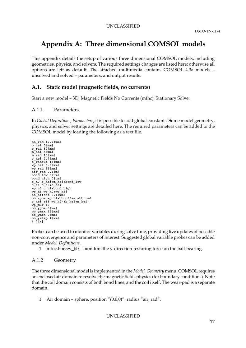
This appendix details the setup of various three dimensional COMSOL models, including geometries, physics, and solvers. The required settings changes are listed here; otherwise all options are left as default. The attached multimedia contains COMSOL 4.3a models – unsolved and solved – parameters, and output results. A.1. Static model (magnetic fields, no currents)
Start a new model – 3D, Magnetic Fields No Currents (mfnc), Stationary Solve. A.1.1 Parameters
In Global Definitions, Parameters, it is possible to add global constants. Some model geometry, physics, and solver settings are detailed here. The required parameters can be added to the COMSOL model by loading the following as a text file. bb_rad 12.7[mm] b_hei 5[mm] b_rad 30[mm] m_hei 5[mm] m_rad 15[mm] c_hei 2.7[mm] c_radout 15[mm] wp_hei 0.8[mm] wp_rad 15[mm] air_rad 0.1[m] bond_low 0[um] bond_high 0[um] c_h0 b_hei+m_hei+bond_low c_h1 c_h0+c_hei wp_h0 c_h1+bond_high wp_h1 wp_h0+wp_hei bb_offset 0.1[mm] bb_zpos wp_h1+bb_offset+bb_rad c_hei_eff wp_h0-(b_hei+m_hei) wp_mur 10 bb_ypos 0[mm] bb_ymax 15[mm] bb_ymin 0[mm] bb_ystep 1[mm] t 0[s]
Probes can be used to monitor variables during solve time, providing live updates of possible non-convergence and parameters of interest. Suggested global variable probes can be added under Model, Definitions.
1. mfnc.Forcey_bb – monitors the y-direction restoring force on the ball-bearing. A.1.2 Geometry
The three dimensional model is implemented in the Model, Geometry menu. COMSOL requires an enclosed air domain to resolve the magnetic fields physics (for boundary conditions). Note that the coil domain consists of both bond lines, and the coil itself. The wear-pad is a separate domain.
1. Air domain – sphere, position “(0,0,0)”, radius “air_rad”.
UNCLASSIFIED 17

UNCLASSIFIED DSTO-TN-1174
2. Base domain – cylinder, position “(0,0,0)”, radius “b_rad”, height “b_hei”. 3. Magnet domain – cylinder, position “(0,0,b_hei)”, radius “m_rad”, height “m_hei”. 4. Coil domain – cylinder, position “(0,0,b_hei+m_hei)”, radius “c_radout”, height
“c_hei_eff”. 5. Wear-pad domain – cylinder, position “(0,0,wp_h0)”, radius “wp_rad”, height
“wp_hei”. 6. Ball-bearing domain – sphere, position “(0,bb_ypos,bb_zpos)”, radius “bb_rad”.
A.1.3 Physics implementation
The material properties for the model are added in the Model, Materials menu, from the Materials Library.
1. Air – selection: all domains. 2. Soft Iron (with losses) – selection: manual, domains “base” and “bearing”.
The physics properties are added to the model with Model, Add Physics (or on initial setup), with the selection for the three dimensional static model being Magnetic Fields, No Currents (mfnc). The properties are added under the MFNC menu.
1. Magnetic Flux Conservation 1 – default (all domains). 2. Magnetic Insulation 1 – default (all boundaries). 3. Initial Values 1 – default (all domains). 4. Magnetic Flux Conservation 2 – selection: “base” and “bearing” domain. Magnetic
Field, Constitutive relation: “BH curve”, Magnetic flux density norm: “from material”. 5. Magnetic Flux Conservation 3 – selection: “magnet” domain. Magnetic Field,
Constitutive relation: “Remanent flux density”, Relative permeability: “from material”, Remanent flux density: “(x,y,z) = (0,0,1.3)”.
6. Magnetic Flux Conservation 4 – selection: “wear-pad” domain. Magnetic Field, Constitutive relation: “Relative permeability”, Relative permeability: “user defined”, “wp_mur”, “Isotropic”.
7. Force Calculation 1 – selection: “bearing” domain. Force name: “bb”, Torque axis: (0,0,1), Torque rotation point: (0,0,0).
Meshing is added in Model, Mesh 1. It is highly geometry dependant, with a goal of a fine mesh on the ball-bearing (for accurate force evaluation) and at least 2-3 layers of elements in other domains for convergence. Given the provided parameters in A.1.1,
1. Free Triangular 1 – selection: “wear-pad” top surface boundary. a. Size 1 – selection: “wear-pad” domain, Element size: custom, Maximum
element size: 1e-3. 2. Swept 1 – selection: “wear-pad” domain, Source faces: “wear-pad” top surface
boundary, Destination faces: “wear-pad” bottom surface boundary. a. Distribution 1 - selection: “wear-pad domain”, Distribution: “Fixed number of
elements”, Number of elements: 3. 3. Convert 1 – selection: “wear-pad” domain, Element split method: “Insert diagonal
edges”.
UNCLASSIFIED 18
UNCLASSIFIED DSTO-TN-1174
4. Free Tetrahedral 1 – selection: all except “wear-pad” domain. a. Size 1 - selection: “bearing” domain, Element size: custom, Maximum element
size: 1.5e-3. b. Size 2 - selection: “coil” domain, Element size: custom, Maximum element size:
3e-3. c. Size 3 - selection: “magnet” domain, Element size: custom, Maximum element
size: 2e-3. d. Size 4 - selection: “base” domain, Element size: custom, Maximum element
size: 3e-3. e. Size 5 - selection: “air” domain, Element size: custom, Maximum element size:
3e-2, Maximum element growth rate: 1.25. A.1.4 Solver configuration
The solver is set up in the Study menu (or on initial setup). Right-click to add a Parametric Sweep, and make sure there is a study step, Step 1: Stationary. Right-click again and select Show default solver.
Parametric sweep: o Sweep parameter: bb_ypos. o Parameter value list: range(bb_ymin,bb_ystep,bb_ymax).
Solver Configurations, Solver 1, Stationary Solver 1: o Left as default. Optional tweaks of direct vs iterative, changing coarse solvers
(MUMPS vs PARDISO), etc for faster solve time with high memory, multi-core machines.
Right-click Study 1 to Compute. Results can be obtained from Data Sets and Derived Values, or in MATLAB with the LiveLink (see Appendix D.1). A plot of “mfnc.Forcey_bb” demonstrates the position dependant restoring force on the ball-bearing. Solve time on an 8-core machine (i7-920 @ 2.67 GHz, 16GB RAM) is approximately 15 minutes. A.2. Transient model (magnetic fields, deformed geometry, global ODEs)
Start a new model – 3D, Magnetic Fields (mf), Deformed Geometry (dg), Global ODEs and DAEs (ge), Stationary Solve. A.2.1 Parameters
In Global Definitions, Parameters, it is possible to add global constants. Some model geometry, physics, and solver settings are detailed here. The required parameters can be added to the COMSOL model by loading the following as a text file. bb_rad 10[mm] b_hei 5[mm] b_rad 30[mm] m_hei 10[mm] m_rad 15[mm]
UNCLASSIFIED 19

UNCLASSIFIED DSTO-TN-1174
c_hei 2[mm] c_radin 5[mm] c_radout 15[mm] cair_rad 20[mm] wp_hei 0.8[mm] wp_rad 15[mm] bb_travel 15[mm] air_rad 0.1[m] bond_low 0[mm] bond_high 0[mm] bb_offset 0.1[mm] c_h0 b_hei+m_hei+bond_low c_h1 c_h0+c_hei wp_h0 c_h1+bond_high wp_h1 wp_h0+wp_hei bb_zpos wp_h1+bb_offset+bb_rad c_hei_eff wp_h0-(b_hei+m_hei) Nturns 198 rho0 1.72e-8[ohm*m] I_step_wid 0.01 t 0[s] wire_rad 127[um] wire_area pi*wire_rad^2 startpos –bb_travel period 1/10
Adding a Function, Analytic allows the ball-bearing displacement to be described.
Function name: bb_displ_cos Expression: (bb_travel*cos(2*pi*1/period*t+pi)-startpos)[m] Arguments: t
Adding a Function, Step allows the soft turn-on of current in the coil to be described. The turn-on is required to allow convergence in the time-dependant solution.
Function name: I_step Location: I_step_wid/2*period From: 0 To: 1 Size of transition zone: I_step_wid*period
Probes can be used to monitor variables during solve time, providing live updates of possible non-convergence and parameters of interest. Suggested global variable probes can be added under Model, Definitions.
1. dg.minqual – monitors the minimum quality of the mesh. 2. mf.mtcd1.Vind – monitors the induced voltage in the coil. 3. Icoil – monitors the current in the coil.
A.2.2 Geometry
The three dimensional model is implemented in the Model, Geometry menu. COMSOL requires an enclosed air domain to resolve the magnetic fields physics (for boundary conditions). Note that the coil domain consists of both bond lines, and the coil itself. The coil is described by multiple geometry domains – the turns of the coil, the inner air gap, and an outer air gap (used to aid mesh movement). A surface is inserted in the coil turn domain perpendicular to the turns, in order to specify coil turn input for Automatic Current Calculation. The wear-pad is not modelled as a domain in this study, due to the fine mesh requirement. The ball-bearing is still offset vertically by the height of the physical wear-pad.
UNCLASSIFIED 20
UNCLASSIFIED DSTO-TN-1174
1. Air domain – sphere, position “(0,0,0)”, radius “air_rad”. 2. Base domain – cylinder, position “(0,0,0)”, radius “b_rad”, height “b_hei”. 3. Magnet domain – cylinder, position “(0,0,b_hei)”, radius “m_rad”, height “m_hei”. 4. Coil domains:
a. Outer coil: cylinder, position “(0,0,b_hei+m_hei)”, radius “cair_rad”, height “c_hei_eff”.
b. Coil turns: cylinder, position “(0,0,b_hei+m_hei)”, radius “c_radout”, height “c_hei_eff”.
c. Inner coil: cylinder, position “(0,0,b_hei+m_hei)”, radius “c_radin”, height “c_hei_eff”.
5. Ball-bearing domain – sphere, position “(0,startpos,bb_zpos)”, radius “bb_rad”. 6. Work Plane 1 – yz-plane, x=0.
a. Plane Geometry – Rectangle 1: width “c_radout-c_radin”, height “c_hei_eff”, Base: Corner, xw “c_radin”, yw “m_hei+b_hei”.
7. Convert to Surface 1 – Input objects: work plane 1. A.2.3 Physics implementation
The material properties for the model are added in the Model, Materials menu, from the pre-existing library.
1. Air – selection: all domains, change Electrical Conductivity to 1[S/m] for convergence. 2. Soft Iron (with losses) – selection: manual, domains “base” and “bearing”.
The physics properties are added to the model with Model, Add Physics (or on initial setup), with the selections for the three dimensional transient model being Magnetic Fields (mf), Deformed Geometry (dg), Global ODEs and DAEs (ge). The properties are added under each physics menu. Note the settings for the coil domain – a current excited multi-turn coil domain, with an Automatic Current Calculation on the Numeric coil type, and the small perturbation to the coil current (1e-9) for convergence. For all physics denoted by (*), right-click and add Gauge Fixing for A-Field. The deformed geometry interface allows all domains to freely deform, then imposes constraints on all boundaries, and finally imposes a time varying displacement on the y-direction of the ball-bearing boundaries. The displacement is in the geometry and mesh, which therefore requires periodic remeshing (handled later in the solvers section). Also note the settings for the global ODEs – the equation “Icoil” calculates the current in the coil, using the induced voltage and the series connection of the coil resistance “mf.mtcd1.R” and a load resistor (in this case, matched to the coil). A smoothing function “I_step” is used to allow soft turn-on convergence. The equation “Vind” simply evaluates the internal induced voltage equation to avoid circular variables issues in the “Icoil” calculation.
1. Magnetic Fields a. Ampere’s Law 1 (*) – default (all domains).
UNCLASSIFIED 21
UNCLASSIFIED DSTO-TN-1174
b. Magnetic Insulation 1 – default (all boundaries). c. Initial Values 1 – default (all domains). d. Ampere’s Law 2 (*) – selection: “base” and “bearing” domain. Magnetic Field,
Constitutive relation: “BH curve”, Magnetic field norm: “from material”. e. Ampere’s Law 3 (*) – selection: “magnet” domain. Magnetic Field,
Constitutive relation: “Remanent flux density”, Relative permeability: “from material”, Remanent flux density: “(x,y,z) = (0,0,1.3)”.
f. Multi-Turn Coil Domain 1 (*) – selection: “coil turn” domain. Coil type: Numeric, Number of turns: “Nturns”, Coil wire cross-section area: “wire_area”, Coil Excitation: Current, Coil Current: “Icoil+1e-9”.
i. Automatic Current Calculation 1 – Off-diagonal scaling: 1 (depending on Coil Investigation result – see solvers section) (option not present in COMSOL 4.3a+).
1. Electric Insulation 1 – selection: all boundaries. 2. Input 1 – selection: “internal coil turns” boundary (created as a
surface converted work plane). g. Force Calculation 1 – selection: “bearing” domain. Force name: “bb”, Torque
axis: (0,0,1), Torque rotation point: (0,0,0). 2. Deformed Geometry
a. Fixed Mesh 1 - default (all domains). b. Prescribed Mesh Displacement 1 - default (all boundaries). c. Free Deformation 1 – selection: all domains. d. Prescribed Mesh Displacement 2 – selection: all boundaries. Prescribed
displacements: “(dx,dy,dz) = (0,0,0)”. e. Prescribed Mesh Displacement 3 – selection: all “bearing” boundaries.
Prescribed displacements: “(dx,dy,dz) = (0,bb_displ_cos(t),0)”. 3. Global ODEs and DAEs
a. Global Equations 1 – add new equations, i. Icoil, Icoil-I_step(t)*Vind/(2*mf.mtcd1.R), 0, 0.
ii. Vind, Vind-mf.mtcd1.Vind, 0, 0. Meshing is added in Model, Mesh 1. It is highly geometry dependant; however solve time in a transient model with many highly coupled physics modes is very long even for moderate size meshes. A course mesh is implemented given the provided parameters in A.2.1. Note the minimum mesh quality with Mesh, Statistics.
1. Free Tetrahedral 1 – selection: all domains. a. Size 1 - selection: “bearing” domain, Element size: custom, Maximum element
size: 8e-3. b. Size 2 - selection: “coil turns”, “coil inner air”, “coil outer air” domains,
Element size: custom, Maximum element size: 3e-3. c. Size 3 - selection: “magnet” domain, Element size: custom, Maximum element
size: 8e-2. d. Size 4 - selection: “base” domain, Element size: custom, Maximum element
size: 5e-3. e. Size 5 - selection: “air” domain, Element size: custom, Maximum element size:
5e-2, Maximum element growth rate: 1.25.
UNCLASSIFIED 22
UNCLASSIFIED DSTO-TN-1174
A.2.4 Solver configuration
The solver is set up in the Study menu (or on initial setup). This model uses 3 separate studies in total, in order to demonstrate stability in the settings. To access the advanced settings in each study after choosing the correct physics, right-click the study and select Show default solver. Note the advanced settings regarding remeshing and maximum time steps – used to ensure that the deforming mesh does not reach a low quality or fail, and that the full transience can occur. Also note that the Segregated Solver in Study 3 is different to the default – the ODE physics calculation must be performed coupled to the MF and Gauge Fixing variables.
Study 1 – Coil: computes the currents in the coil to determine coil directions (ensures correct path).
o Steps Step 1: Coil Current Calculation
Coil name: 1. Physics and variables selection: Magnetic Fields only.
o Solver Configurations: default. o Results: plot of “mf.mtcd1.eCoil” streamlines (on internal boundary surface)
demonstrates current path in the coil. This path should be roughly circular – changing Off-diagonal scaling in the Numeric coil settings changes the path. Note that as of COMSOL 4.3a, off-diagonal scaling is automatic.
o Update the model and use the new settings in Study 2. Study 2 – DG: computes the transient movement of the geometry with no physics
(ensures no remeshing problems). o Steps
Step 1: Stationary Physics and variables selection: Deformed geometry only.
Step 2: Time Dependent Times: range(0,0.003,0.25)*period. Physics and variables selection: Deformed geometry only. Study Extensions: Automatic Remeshing enabled.
o Solver Configurations: default. Time-Dependent Solver 1
Time Stepping - Maximum Step: 0.003*period. Automatic Remeshing - Minimum mesh quality: 0.04,
Consistent Initialization: Backward Euler. Fully Coupled 1 – Termination: Iterations, Iterations: 1.
o Results: plot of “qual” as a slice through x=0 shows the mesh quality as the ball-bearing moves in the transient solution (useful to set Results While Solving for live plots). The volume immediately under the ball-bearing is generally the point of failure. Ensure that the deforming geometry and automatic remeshing technique solves for the entire time range (without back-stepping). Altering the mesh, the maximum step time, and the automatic remeshing minimum quality will tune the model to allow solving.
UNCLASSIFIED 23
UNCLASSIFIED DSTO-TN-1174
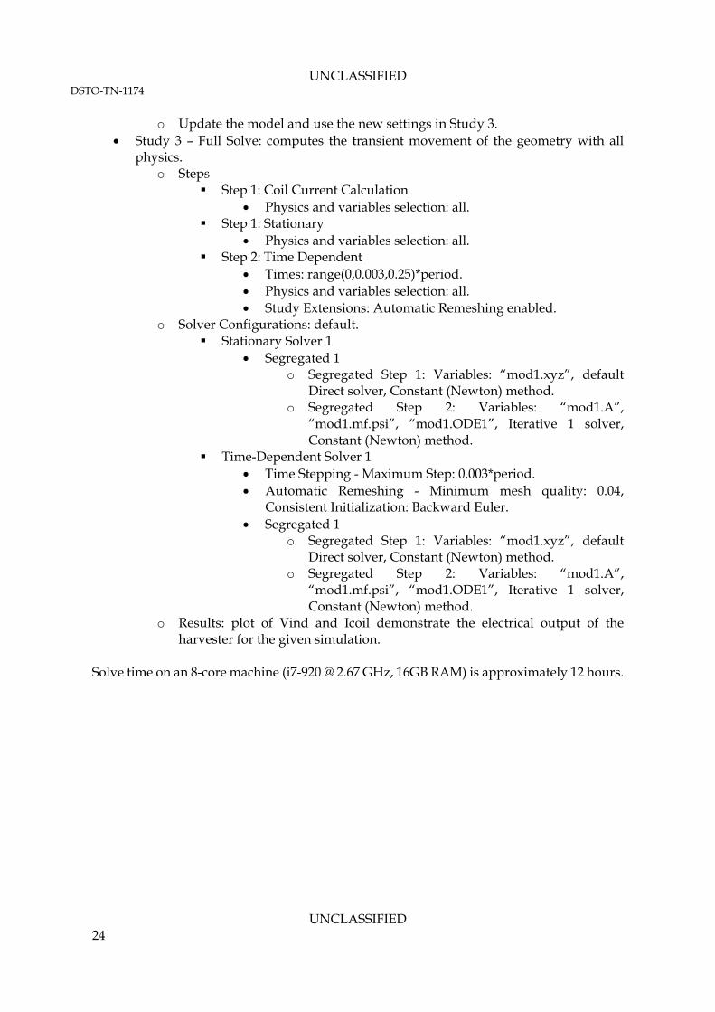
o Update the model and use the new settings in Study 3. Study 3 – Full Solve: computes the transient movement of the geometry with all
physics. o Steps
Step 1: Coil Current Calculation Physics and variables selection: all.
Step 1: Stationary Physics and variables selection: all.
Step 2: Time Dependent Times: range(0,0.003,0.25)*period. Physics and variables selection: all. Study Extensions: Automatic Remeshing enabled.
o Solver Configurations: default. Stationary Solver 1
Segregated 1 o Segregated Step 1: Variables: “mod1.xyz”, default
Direct solver, Constant (Newton) method. o Segregated Step 2: Variables: “mod1.A”,
“mod1.mf.psi”, “mod1.ODE1”, Iterative 1 solver, Constant (Newton) method.
Time-Dependent Solver 1 Time Stepping - Maximum Step: 0.003*period. Automatic Remeshing - Minimum mesh quality: 0.04,
Consistent Initialization: Backward Euler. Segregated 1
o Segregated Step 1: Variables: “mod1.xyz”, default Direct solver, Constant (Newton) method.
o Segregated Step 2: Variables: “mod1.A”, “mod1.mf.psi”, “mod1.ODE1”, Iterative 1 solver, Constant (Newton) method.
o Results: plot of Vind and Icoil demonstrate the electrical output of the harvester for the given simulation.
Solve time on an 8-core machine (i7-920 @ 2.67 GHz, 16GB RAM) is approximately 12 hours.
UNCLASSIFIED 24

UNCLASSIFIED DSTO-TN-1174
Appendix B: Harvester ball-bearing dynamics
B.1. Homotopy analysis method
Recalling the nonlinear differential equation (4) in terms of new parameters,
,t (A1)
)()( Atu , (A2)
,)cos()(')('
)(')(')(5
553
33
12
akAkA
kAAA
(A3)
From Liao and Tan [22], we construct a homotopy composed of linear and nonlinear operators (denoted by L and N respectively), with a parameter q denoting the embedding parameter responsible for the homotopy,
)](),;([)]();([)1(]),;([ 0 qqqNqLqqqH , (A4)
0q :
)]()0;([]0),0;([ 0 LH , (A5)
1q :
)]1(),1;([]1),1;([ NH . (A6)
As the embedding parameter changes from 0 to 1, );( q deforms from the initial guess
)(0 to the solution )( , and from an unknown initial amplitude to the solution . Provided proper selection of auxiliary control parameter , the convergent series solution takes the form,
)(q 0A A
,)()()(0
0
nn (A7)
.1
0
n
nAAA (A8)
The base function of Ψ(τ) is selected as a sinusoidal function,
),cos()(0 (A9)
UNCLASSIFIED 25
UNCLASSIFIED DSTO-TN-1174
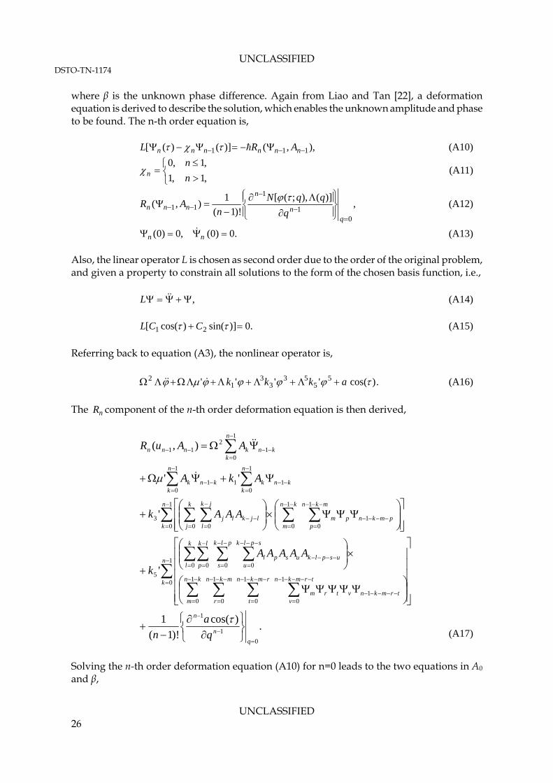
where β is the unknown phase difference. Again from Liao and Tan [22], a deformation equation is derived to describe the solution, which enables the unknown amplitude and phase to be found. The n-th order equation is,
),,()]()([ 111 nnnnnn ARL (A10)
,1,1
,1,0
n
nn (A11)
,)](),;([
)!1(
1),(
01
1
11
q
n
n
nnnq
qqN
nAR
(A12)
.0)0(,0)0( nn (A13)
Also, the linear operator L is chosen as second order due to the order of the original problem, and given a property to constrain all solutions to the form of the chosen basis function, i.e.,
, L (A14)
.0)]sin()cos([ 21 CCL (A15)
Referring back to equation (A3), the nonlinear operator is,
.)cos('''' 55
533
31
2 akkk (A16)
The component of the n-th order deformation equation is then derived, nR
.)cos(
)!1(
1
'
'
''
),(
0
1
1
1
0 1
0
1
0
1
0
1
01
0 0 0 0
5
1
0
1
0
1
01
0 03
1
011
1
01
1
01
211
q
n
n
n
k kn
m
mkn
r
rmkn
t
trmkn
vtrmknvtrm
k
l
lk
p
plk
s
splk
uusplkuspl
n
k
kn
m
mkn
ppmknpm
k
j
jk
lljklj
n
kknk
n
kknk
n
kknknnn
q
a
n
AAAAA
k
AAAk
AkA
AAuR
(A17)
Solving the n-th order deformation equation (A10) for n=0 leads to the two equations in A0 and β,
UNCLASSIFIED 26

UNCLASSIFIED DSTO-TN-1174
,'8
'5
4
'3' 22
022
2405
2032
1 aAAkAk
k
(A18)
405
203
21 '5'6)'(8
'8)tan(
AkAkk
. (A19)
Taking n=1 in equation (A10) for the first order deformation,
.))(5cos())(3cos(516
'
))(3cos(4
')()(
2
505
2
303
11
Ak
Ak
(A20)
Continual deformations can be calculated iteratively. The 1st order solution of u(t) is calculated by solving equation (A20) for )(1 , solving equation (A18) for A0, and substituting these into equation (A2),
.5cos384
'3cos
128
'5
3cos32
'cos)(
2
505
2
505
2
303
0
tAk
tAk
tAk
tAtu
(A21)
Mathematica software can be used to automate the iteration process, however as described in section 2.2.1.1, only the 1st order solution was deemed necessary.
UNCLASSIFIED 27
UNCLASSIFIED DSTO-TN-1174
Appendix C: Vibro-impact dynamics
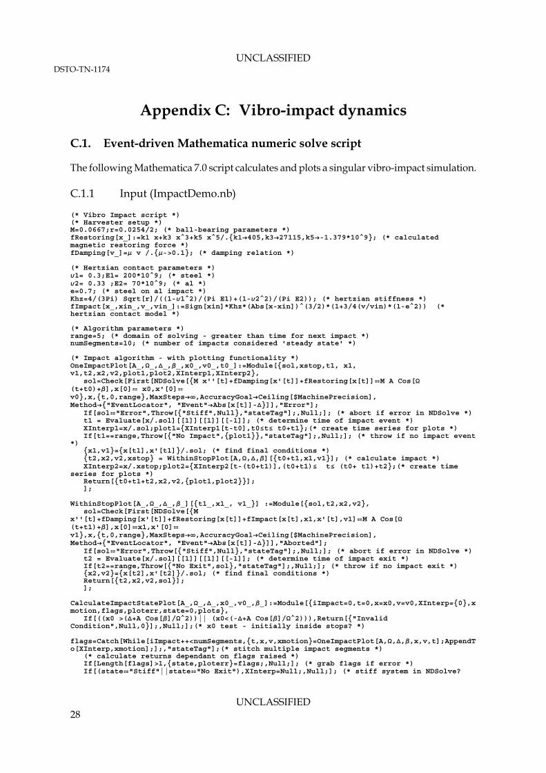
C.1. Event-driven Mathematica numeric solve script
The following Mathematica 7.0 script calculates and plots a singular vibro-impact simulation. C.1.1 Input (ImpactDemo.nb)
(* Vibro Impact script *) (* Harvester setup *) M=0.0667;r=0.0254/2; (* ball-bearing parameters *) fRestoring[x_]:=k1 x+k3 x^3+k5 x^5/.k1405,k327115,k5-1.379*10^9; (* calculated magnetic restoring force *) fDamping[v_]= v /.->0.1; (* damping relation *) (* Hertzian contact parameters *) 1= 0.3;E1= 200*10^9; (* steel *) 2= 0.33 ;E2= 70*10^9; (* al *) e=0.7; (* steel on al impact *) Khz=4/(3Pi) Sqrt[r]/((1-1^2)/(Pi E1)+(1-2^2)/(Pi E2)); (* hertzian stiffness *) fImpact[x_,xin_,v_,vin_]:=Sign[xin]*Khz*(Abs[x-xin])^(3/2)*(1+3/4(v/vin)*(1-e^2)) (* hertzian contact model *) (* Algorithm parameters *) range=5; (* domain of solving - greater than time for next impact *) numSegments=10; (* number of impacts considered 'steady state' *) (* Impact algorithm - with plotting functionality *) OneImpactPlot[A_,_,_,_,x0_,v0_,t0_]:=Module[sol,xstop,t1, x1, v1,t2,x2,v2,plot1,plot2,XInterp1,XInterp2, sol=Check[First[NDSolve[M x''[t]+fDamping[x'[t]]+fRestoring[x[t]]M A Cos[ (t+t0)+],x[0] x0,x'[0] v0,x,t,0,range,MaxSteps,AccuracyGoalCeiling[$MachinePrecision], Method"EventLocator", "Event"Abs[x[t]]-]],"Error"]; If[sol"Error",Throw["Stiff",Null,"stateTag"];,Null;]; (* abort if error in NDSolve *) t1 = Evaluate[x/.sol][[1]][[1]][[-1]]; (* determine time of impact event *) XInterp1=x/.sol;plot1=XInterp1[t-t0],t0t t0+t1;(* create time series for plots *) If[t1==range,Throw["No Impact",plot1,"stateTag"];,Null;]; (* throw if no impact event *) x1,v1=x[t1],x'[t1]/.sol; (* find final conditions *) t2,x2,v2,xstop = WithinStopPlot[A,,,][t0+t1,x1,v1]; (* calculate impact *) XInterp2=x/.xstop;plot2=XInterp2[t-(t0+t1)],(t0+t1) t (t0+ t1)+t2;(* create time series for plots *) Return[t0+t1+t2,x2,v2,plot1,plot2]; ]; WithinStopPlot[A_,_,_,_][t1_,x1_, v1_] :=Module[sol,t2,x2,v2, sol=Check[First[NDSolve[M x''[t]+fDamping[x'[t]]+fRestoring[x[t]]+fImpact[x[t],x1,x'[t],v1]M A Cos[ (t+t1)+],x[0]x1,x'[0] v1,x,t,0,range,MaxSteps,AccuracyGoalCeiling[$MachinePrecision], Method"EventLocator", "Event"Abs[x[t]]-]],"Aborted"]; If[sol"Error",Throw["Stiff",Null,"stateTag"];,Null;]; (* abort if error in NDSolve *) t2 = Evaluate[x/.sol][[1]][[1]][[-1]]; (* determine time of impact exit *) If[t2==range,Throw["No Exit",sol,"stateTag"];,Null;]; (* throw if no impact exit *) x2,v2=x[t2],x'[t2]/.sol; (* find final conditions *) Return[t2,x2,v2,sol]; ]; CalculateImpactStatePlot[A_,_,_,x0_,v0_,_]:=Module[iImpact=0,t=0,x=x0,v=v0,XInterp=0,xmotion,flags,ploterr,state=0,plots, If[((x0 >(+A Cos[]/^2))|| (x0<(-+A Cos[]/^2))),Return["Invalid Condition",Null,0];,Null;];(* x0 test - initially inside stops? *) flags=Catch[While[iImpact++<numSegments,t,x,v,xmotion=OneImpactPlot[A,,,,x,v,t];AppendTo[XInterp,xmotion];];,"stateTag"];(* stitch multiple impact segments *) (* calculate returns dependant on flags raised *) If[Length[flags]>1,state,ploterr=flags;,Null;]; (* grab flags if error *) If[(state"Stiff"||state"No Exit"),XInterp=Null;,Null;]; (* stiff system in NDSolve?
UNCLASSIFIED 28

UNCLASSIFIED DSTO-TN-1174
error in exit return? *) If[(state"No Impact"),AppendTo[XInterp,ploterr];t=t+range;,Null;]; (* not steady-state? append final time series to segments *) If[(state"No Impact"&&iImpact>1&&iImpact<numSegments),state="Transient";,Null;];(* add state for transient impacting *) If[(iImpact numSegments),state="Steady State";,Null;]; (* add state for steady state impacting *) If[Length[XInterp]0,plots=Null;,plots=Piecewise[Flatten[XInterp[[2;;]],1]];]; (* compile plots *) Return[state,plots,t]; ]; (* Variables for testing *) Atemp=0.5*9.81*Sqrt[2]; (* base acceleration *) temp=12*2*Pi; (* base frequency *) x0temp=0; (* initial x *) v0temp=0; (* initial v *) temp=0;(* initial phase *) temp=0.0055;(* gap size *) (* Calculate and plot time series *) time,state,timeSeries,tEnd=Timing[CalculateImpactStatePlot[Atemp,temp,temp,x0temp,v0temp,temp]]; Print["State: ",state, " - calc in ",time,"s"]; XInterp[t0_]:=Evaluate[timeSeries/.tt0] Plot[XInterp[t],temp,-temp,t,0,tEnd]
C.1.2 Output
Example output is shown in Figure C1.
State: Steady State - calc in 0.062 s
0.2 0.4 0.6 0.8
-0.004
-0.002
0.002
0.004
Figure C1 Example output for event-driven vibro-impact simulation script, for provided test variables. Includes determined state, time for execution, and plot of relative ball-bearing displacement. C.2. Calculation parallelisation script
The following Mathematica 7.0 script calculates vibro-impact states over multiple variables on multiple kernels. It assumes that the variables defined in Appendix C.1 are available. Provided is the initial condition selection algorithm – related to steady-state conditions at the operating mode, briefly described in section 2.2.2. C.2.1 Input (ParallelImpactScript.nb)
(* Set up kernels *)
UNCLASSIFIED 29

UNCLASSIFIED DSTO-TN-1174
CloseKernels[];LaunchKernels[$ProcessorCount]; $ConfiguredKernels (* show number of kernels *) 8 local kernels (* Functions and definitions *) (* create equivalent Duffing spring *) =fDamping[v]/v; k1,k3,k5=CoefficientList[fRestoring[x],x][[2;;;;2]]; yMax=0.015;yStep=0.001;ClearAll[,]; ,=,/.FindFit[Table[y,k1 y+k3 y^3+k5 y^5,y,0,yMax,yStep], y + y^3,,,y]; (* Possible initial conditions *) maxDispl[_,_,F_,_,_]:=Max[Select[A/.NSolve[(((/M)-^2+3 (/M)/4 A^2)^2+(/M)^2 ^2) A^2-F^20,A],Im[#]0&]]; maxVel[_,_,F_,_,_]:= maxDispl[,,F,,]; initList[max_]:=Range[-max,max,2max/(nSamples-1)]; (* Bool - in possible region of initial conditions *) inEllipse[ini_,xmax_,vmax_,_]:=Module[x=ini[[1]],v=ini[[2]], If[((((x/Abs[xmax])^2+(v/Abs[vmax])^2)1)&&Abs[x] ),Return[1];,Return[0];]; ]; (* Get elliptical initial condition list from square list *) filterEllipse[xList_,vList_,xmax_,vmax_,_]:=Module[initList,boolEllipse, initList=Flatten[Table[xList[[i]],vList[[j]],i,1,Length[xList],j,1,Length[vList]],1]; boolEllipse=MapThread[inEllipse,initList,ConstantArray[xmax,Length[initList]],ConstantArray[vmax,Length[initList]],ConstantArray[,Length[initList]]]; Select[initList*boolEllipse,#0,0&]//Return; ]; (* Get initial conditions from given drive level *) initCondsAtDrive[A_,_,_]:=Module[xmax,vmax,vinitSquare,xinitSquare, (* find max values from HBM *) xmax=maxDispl[,,A,,]; vmax=maxVel[,,A,,]; (* create a square list of initial conditions *) If[xmax<,xinitSquare=initList[xmax];,xinitSquare=initList[];]; vinitSquare=initList[vmax]; (* mask square list by -modified ellipse filter for possible initial conditions *) filterEllipse[xinitSquare,vinitSquare,xmax,vmax,]//Return; ]; (* Create list of initial conditions to calculate *) initConds[conds_]:=Module[A=conds[[1]],=conds[[2]],=conds[[3]],=conds[[4]],xList,vList,initList, initList=initCondsAtDrive[A,,]; Table[A,,,,initList[[i]][[1]],initList[[i]][[2]],i,1,Length[initList]]//Return; ]; (* Create variables for testing *) (* Sweep parameters *) AList=0.5* Sqrt[2]*9.81; (* base acceleration *) List=Table[i*2*Pi,i,10,20,0.1]; (* frequency range *) List=Range[0,7Pi/4,Pi/4]; (* mass-base phase difference *) List=3,6,8,12,15*10^-3; (* gap sizes *) nSamples=10; (* n x n x/v initial condition grid *) (* Create a variable list with harvester properties *) varList=Tuples[AList,List,List,List]; (* combinations of parameters in varList - for ParallelDo *) varList=Flatten[initConds/@varList,1];(* Obtain parameter list with phase properties for algorithm, by analysing possible conditions exist in ellipse governed by HBM *) solList=Range[1,Length[varList]]; (* solution numbers for external saving *) pad=StringLength[ToString[solList[[-1]]]]; (* padding for consistent file naming *) outputDirectory=NotebookDirectory[]<>"data\\Parallel\\"; (* Make constants, functions, parameters, varList, solList available to multiple kernels *) DistributeDefinitions[M,e,r,k1,k3,k5,,Khz,fDamping,fRestoring,fImpact, range,numSegments,OneImpactPlot,WithinStopPlot,CalculateImpactStatePlot,varList,solList,pad,outputDirectory]; Print["Number of solutions: ", solList[[-1]]]; Number of solutions: 266496 (* Begin counter *) timer=AbsoluteTime[];
UNCLASSIFIED 30
UNCLASSIFIED DSTO-TN-1174
(* Start parallel loops *) ParallelDo[ (* Assign variables *) Atemp,temp,temp,temp,x0temp,v0temp=varList[[iVar]]; (* Code block - evaluate functions and obtain result for saving *) state,timeSeries,tEnd=CalculateImpactStatePlot[Atemp,temp,temp,x0temp,v0temp,temp]; (* Export to external text file *) Export[outputDirectory<>ToString@NumberForm[solList[[iVar]],pad,NumberPadding"0",""] <> ".dat", ToString[Row[N[varList[[iVar]]],","]]<>","<>state<>"\n","Text"]; ,iVar,1,Length[varList]] (* display final time *) Print["Calc time: ",N[AbsoluteTime[]-timer],"s"]; Print["Time per solution: ",N[AbsoluteTime[]-timer]/solList[[-1]],"s"];
C.2.2 Output
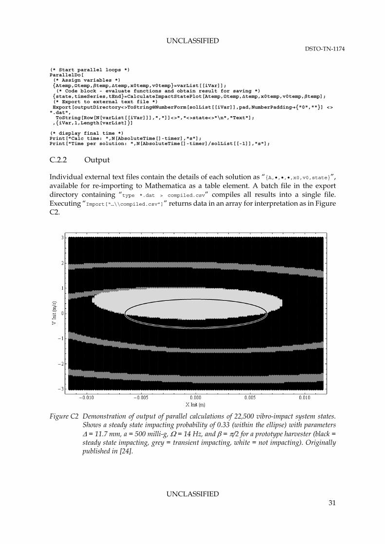
Individual external text files contain the details of each solution as “A,•,•,•,x0,v0,state”, available for re-importing to Mathematica as a table element. A batch file in the export directory containing “type *.dat > compiled.csv” compiles all results into a single file. Executing “Import[“…\\compiled.csv”]” returns data in an array for interpretation as in Figure C2.
Figure C2 Demonstration of output of parallel calculations of 22,500 vibro-impact system states. Shows a steady state impacting probability of 0.33 (within the ellipse) with parameters = 11.7 mm, a = 500 milli-g, = 14 Hz, and = /2 for a prototype harvester (black = steady state impacting, grey = transient impacting, white = not impacting). Originally published in [24].
UNCLASSIFIED 31

UNCLASSIFIED DSTO-TN-1174
C.2.3 Computation comparison
Table C1 indicates that a speed increase of 5.3 is possible through parallelisation of the Mathematica script (as shown in Appendix C.2.1). Table C1 Comparison of sequential and parallel computation – demonstrating a 5.3 times increase in
computation speed
Calculation method Solutions Total time (s) Time per solution (s) Sequential 5000 307.5 0.0615 Parallel 5000 58.3 0.0117
UNCLASSIFIED 32
UNCLASSIFIED DSTO-TN-1174
Appendix D: Electromagnetic transduction
D.1. Model data extraction in MATLAB (modelExporter_main.m)
The following script extracts data from a COMSOL model loaded onto the MATLAB server, for use in Mathematica. str_modelname = 'H27'; % model name on COMSOL server model = ModelUtil.model(str_modelname); studyval='std6'; datasetval='dset2'; % values in COMSOL solve % Obtain set parameters from model c_hei = removeUnits(model.param.get('c_hei')); c_radout = removeUnits(model.param.get('c_radout')); b_hei = removeUnits(model.param.get('b_hei')); m_hei = removeUnits(model.param.get('m_hei')); bond_low = removeUnits(model.param.get('bond_low')); bond_high = removeUnits(model.param.get('bond_high')); c_h0 = b_hei+m_hei+bond_low; c_h1 = c_h0+c_hei; % parametric sweep details: 'Outersolnum' y_max = removeUnits(model.param.get('bb_ymax')); y_min = removeUnits(model.param.get('bb_ymin')); y_step = removeUnits(model.param.get('bb_ystep')); paramList=y_min:y_step:y_max; paramvals=1:length(paramList); c_radout_nom=y_max; % assume solved out to edge of coil % various algorithm parameters comsolInterpRes=2e-4; % distance between interpolated points in coil region - reasonable w.r.t. mesh quality & wire diam rho_wire=1.68e-8; % copper resistivity % define Bz evaulation region [x,x,y,y,z,z] coilRegion=[-c_radout_nom,c_radout_nom,-c_radout_nom,c_radout_nom,c_h0,c_h1]; % Export Fy dynamics to CSV exportForces(model,datasetval,paramList,['data\', str_modelname]); % Obtain flux density from Comsol model and export to CSV % Interpolates flux in entire coil region over all parametric solutions struct_FluxDensity=interpFluxDensity(model,datasetval,paramList,coilRegion,comsolInterpRes); exportFluxDensity(struct_FluxDensity,['data\', str_modelname]); %% Functions %% ---------------------------------------------- %% exportFluxDensity % exports Comsol Bz fields to a csv for varying parameters function exportFluxDensity(struct_FluxDensity,exportStr) csvwrite([exportStr,'_flux_xi.csv'],struct_FluxDensity.xi); csvwrite([exportStr,'_flux_yi.csv'],struct_FluxDensity.yi); csvwrite([exportStr,'_flux_zi.csv'],struct_FluxDensity.zi); csvwrite([exportStr,'_flux_param.csv'],struct_FluxDensity.param); for i=1:size(struct_FluxDensity.Bz,1) csvwrite([exportStr,'_flux_bz_',num2str(i),'.csv'],struct_FluxDensity.Bzi,1); end end %% exportForces % exports Comsol Fx/Fy/Fz to a csv function [mat_Fx,mat_Fy,mat_Fz]=exportForces(model,datasetval,paramList,exportStr) % extract BB_Fy for each parameter point % parametric sweep: 'Outersolnum' paramvals=1:length(paramList); mat_Fx=zeros(length(paramvals),2); mat_Fx(:,1)=paramList'; mat_Fy=mat_Fx; mat_Fz=mat_Fx; h_wait=waitbar(0,'Waitbar'); tic; % waitbar for i_param=paramvals
UNCLASSIFIED 33
UNCLASSIFIED DSTO-TN-1174
mat_Fx(i_param,2)=mphglobal(model,'mfnc.Forcex_bb','dataset',datasetval,'Outersolnum',i_param); mat_Fy(i_param,2)=mphglobal(model,'mfnc.Forcey_bb','dataset',datasetval,'Outersolnum',i_param); mat_Fz(i_param,2)=mphglobal(model,'mfnc.Forcez_bb','dataset',datasetval,'Outersolnum',i_param); % Update waitbar waitbar(i_param/length(paramvals), h_wait, ['Approximate time to completion: ', ... int2str(ceil((length(paramvals)-i_param)/i_param*toc)), ' s']); end csvwrite([exportStr,'_fx.csv'],mat_Fx); csvwrite([exportStr,'_fy.csv'],mat_Fy); csvwrite([exportStr,'_fz.csv'],mat_Fz); close(h_wait); end %% ---------------------------------------------- %% interpFluxDensity % uses mphinterp to evaulate mfnc.Bz at each point in coil region % returns cell of Bz at x,y,z function [struct_FluxDensity]=interpFluxDensity(model,datasetval,paramList,coilRegion,interpRes) c_x0=coilRegion(1); c_x1=coilRegion(2); c_y0=coilRegion(3); c_y1=coilRegion(4); c_z0=coilRegion(5); c_z1=coilRegion(6); % matrix of x,y,z points xArr=linspace(c_x0,c_x1,(c_x1-c_x0)/interpRes); yArr=linspace(c_y0,c_y1,(c_y1-c_y0)/interpRes); zArr=linspace(c_z0,c_z1,(c_z1-c_z0)/interpRes); pointsX=length(xArr); pointsY=length(yArr); pointsZ=length(zArr); % create 3D array of points [xi,yi,zi]=meshgrid(xArr,yArr,zArr); % condition into nDim x nPoints array for Comsol mat_Points=zeros(3,pointsX*pointsY*pointsZ); count=0; for i=1:pointsX for j=1:pointsY for k=1:pointsZ count=count+1; mat_Points(1,count)=xArr(i); mat_Points(2,count)=yArr(j); mat_Points(3,count)=zArr(k); end end end % calculate flux density for each parameter point % mphinterp returns ntime x nPoints array % parametric sweep: 'Outersolnum' paramvals=1:length(paramList); cell_fluxDensity=cell(length(paramvals),1); h_wait=waitbar(0,'Waitbar'); tic; for i_param=paramvals cell_fluxDensityi_param,1=mphinterp(model,'mfnc.Bz','coord',mat_Points,'dataset',datasetval,'Outersolnum',i_param); % Update waitbar waitbar(i_param/length(paramvals), h_wait, ['Approximate time to completion: ', ... int2str(ceil((length(paramvals)-i_param)/i_param*toc)), ' s']); end % condition from Comsol array into 3D array for i_param=paramvals fluxDensity1D=cell_fluxDensityi_param,1; fluxDensity3D=zeros(pointsX,pointsY,pointsZ); count=0; for i=1:pointsX for j=1:pointsY for k=1:pointsZ count=count+1; fluxDensity3D(i,j,k)=fluxDensity1D(count); end end end cell_FluxDensityi_param,1=fluxDensity3D;
UNCLASSIFIED 34

UNCLASSIFIED DSTO-TN-1174
end % store in struct for return struct_FluxDensity=struct('xi',xi,'yi',yi,'zi',zi,'param',paramList,'Bz',cell_FluxDensity); close(h_wait); end %% ---------------------------------------------- %% removeUnits % Remove units from COMSOL strings function [val]=removeUnits(str) temp=char(str); for i=1:length(temp) if(temp(i)=='[') break; end end % Convert units factor=1; if(temp(i+1:i+2)=='mm') factor=1/1000; end if(temp(i+1:i+2)=='um') factor=1/1000000; end val=str2num(temp(1:i-1))*factor; end
D.2. Numeric coil output Mathematica script
The following Mathematica 7.0 script calculates output of a harvester numerically, from COMSOL data. The user can configure the coil arrangement, and determine output given any displacement function or response (including the 2DOF x-y plane arrangement). It requires the exported files created in MATLAB by the script in Appendix D.1. The example output is for a two coil arrangement. The script requires the use of an open-source package called “Obtuse Angle Interpolation” (online: www.familydahl.se/mathematica). D.2.1 Input (InducedVoltage.nb)
(* Set up kernels *) CloseKernels[];LaunchKernels[$ProcessorCount]; $ConfiguredKernels (* show number of kernels *) 8 local kernels (* Import param list of COMSOL solutions *) datadir=NotebookDirectory[]<> "\\data\\"; modelname="H27_"; str1=datadir<>modelname; paramList=Import[str1 <> "flux_param.csv"][[1]]; paramList=Select[Transpose[Range[1,Length[paramList]],paramList],Sign[#[[2]]]0&]; (* get only positive displacement solutions *) paramFileIndexes,paramList=Transpose[paramList]; (* Import x,y,z *) xList,yList,zList=Import[str1 <>#]&/@ "flux_xi.csv", "flux_yi.csv", "flux_zi.csv"; (* Import Bz *) resortBz[data_,yi_]:=Partition[data,yi]//Transpose; importBz[param_,xi_,yi_]:=MapThread[resortBz,Import[str1 <> "flux_bz_" <> ToString[param] <> ".csv"],ConstantArray[yi,xi]]; bzList=MapThread[importBz,paramFileIndexes,ConstantArray[Length[xList],Length[paramList]],ConstantArray[Length[yList],Length[paramList]]]; (* Sample plot *) ncontours=10; ListContourPlot3D[bzList[[-1]],Contoursncontours,MeshNone,ContourStyleTable[Lighter[Red,i/ncontours],i,1,ncontours],ImageSize300] (* Obtain 3D interpolation functions for each Bz field *) (* sort data into x,y,z,Bz *) coords=Tuples[DeleteDuplicates/@Flatten/@xList,yList,zList]; insertCoordinates[data_]:=(#[[1]],#[[2]])&/@Transpose[coords,Flatten[data]] (* Place coordinates in data and interpolate *)
UNCLASSIFIED 35
UNCLASSIFIED DSTO-TN-1174
bzData=insertCoordinates/@bzList; bzFun=Interpolation/@bzData; (* Rotating Bz solutions for an x-y ball-bearing position solution - take advantage of cylindrical magnet radial symmetry *) nPoints=50; maxRadius=Max[paramList]; (* Use rotation transform on a varying set of points *) getRadialPoints[r_]:=If[r0,0,0,Tuples[Table[i,i,0,2Pi,2Pi/(r/maxRadius*nPoints)],r]]; (* Get polar values *) xyPlanePolar=Flatten[getRadialPoints/@paramList,1]; Print["nPoints: ",Length[xyPlanePolar]]; ListPolarPlot[xyPlanePolar,ImageSize300] (* Get x-y values from polar coords *) getXYPoints[_,r_]:=First[Re[#],Im[#]&/@r*Exp[ ]] xyPlane=getXYPoints/@xyPlanePolar; nPoints: 411 (* Rotational transform to get x/y grid of flux values *) rotTransform[_]:=RotationTransform[,0,0,1,0,0,0] (* rotate z about 0,0,0 *) (* Given a polar point, obtain Bz field *) lookupBz[r_]:=Select[Transpose[Range[1,Length[paramList]],paramList],#[[2]]r&][[1]][[1]] transformFunction[fun_,_,x_,y_,z_]:=fun[u,v,w]/.Thread[u,v,w->rotTransform[][x,y,z]] obtainBz[_,r_]:=transformFunction[bzFun[[lookupBz[r]]],,x,y,z] (* Set up some coil parameters *) chei=Max[zList]-Min[zList];(* Specified in COMSOL *) rho=1.68*10^-8;wireradcu=133*10^-6;wirerad=150*10^-6; cuarea=Pi wireradcu^2; (* functions for resistance calcs *) loopResistance[r_]:=rho/cuarea*2Pi r; calcCoilResistance[offset_,rset_,hset_]:=Module[Rwires=loopResistance/@rset, Length[hset]*Sum[Rwires[[i]],i,Length[Rwires]]//Return; ]; (* calc total turns *) calcCoilTurns[offset_,rset_,hset_]:=Length[hset]*Length[rset] (* Best fit of unit circles in a circle - 1-9 circles *) circlelist= 0.,0., 1.,0.,-1.,0., 0.,1.1547,-1.,-0.57735,1.,-0.57735, 1.,1.,-1.,1.,-1.,-1.,1.,-1., 1.61803,0.52573,0.,1.7013,-1.61803,0.52573,-1.,-1.37638,1.,-1.37638, 2.,0.,1.,1.73205,-1.,1.73205,-2.,0.,-1.,-1.73205,1.,-1.73205, 0.,0.,2.,0.,1.,1.73205,-1.,1.73205,-2.,0.,-1.,-1.73205,1.,-1.73205, 0.,0.,1.80194,1.437,0.,2.30476,-1.80194,1.437,-2.24698,-0.51286,-1.,-2.07652,1.,-2.07652,2.24698,-0.51286,0.,0.,2.41421,1.,1.,2.41421,-1.,2.41421,-2.41421,1.,-2.41421,-1.,-1.,-2.41421,1.,-2.41421,2.41421,-1. ; (* Create some coils based on circle fits *) createSingleCoil[chei_,crout_,crin_,x_,y_]:=Module[rset,hset, rset=Table[i,i,crin+wirerad,crout-wirerad,wirerad*2]; hset=Table[i+Min[Flatten[zList]],i,wirerad,chei-wirerad,wirerad*2]; Return[x,y,rset,hset]; ]; createCoils[NCoils_,chei_,crin_,maxradius_]:=Module[centres=circlelist[[NCoils]],rCoils,rlarge,params,coilCentres, rlarge=Norm[Last[SortBy[centres,Norm]]] +1; rCoils=maxradius/rlarge; coilCentres=#*rCoils&/@centres; params=MapThread[ConstantArray,chei,rCoils,crin,ConstantArray[NCoils,3]]; MapThread[createSingleCoil,params[[1]],params[[2]],params[[3]],coilCentres] ]; (* create a coil and plot it *) maxRadius=Max[paramList]; testCoil=createCoils[2,chei,0.003,maxRadius]; coilResistances=calcCoilResistance/@testCoil; coilTurns=calcCoilTurns/@testCoil; Print["Resistances: ",coilResistances," Sum: ", Total[coilResistances]]; Print["Turns: ",coilTurns," Sum: ", Total[coilTurns]]; plotCoil[offset_,rset_,hset_]:=Show[Table[ContourPlot[(x-offset[[1]])^2+(y-offset[[2]])^2==crad^2,x,-maxRadius,maxRadius,y,-maxRadius,maxRadius,PlotRangeAll],crad,rset],PlotRangeAll] Show[plotCoil/@testCoil,ContourPlot[(x)^2+(y)^2==Max[paramList]^2,x,-
UNCLASSIFIED 36

UNCLASSIFIED DSTO-TN-1174
maxRadius,maxRadius,y,-maxRadius,maxRadius,ContourStyleBlack,Thick],PlotRangeAll] Resistances: 1.34626,1.34626 Sum: 2.69252 Turns: 135,135 Sum: 270 (* Compute flux in a coil for a specified ball-bearing position *) getPointFluxCoil[_,r_,offset_,rset_,hset_]:=Module[polarBzFun=obtainBz[,r], Print[,r]; Sum[Quiet[NIntegrate[Boole[(x-offset[[1]])^2+(y-offset[[2]])^2 crad^2]*polarBzFun,x,-maxRadius,maxRadius,y,-maxRadius,maxRadius,z,Min[hset],Max[hset],AccuracyGoal7,MethodLocalAdaptive]],crad,rset]*Length[hset]/(Max[hset]-Min[hset]) ] (* compute across XY polar points in parallel *) DistributeDefinitions[getPointFluxCoil,xyPlanePolar,testCoil,obtainBz,maxRadius,lookupBz,paramList,bzFun,transformFunction,rotTransform]; getXYFluxCoil[offset_,rset_,hset_]:=Parallelize[MapThread[getPointFluxCoil,xyPlanePolar,ConstantArray[offset,rset,hset,Length[xyPlanePolar]]]]; iCoil=1; Show[plotCoil[testCoil[[iCoil]]],ContourPlot[(x)^2+(y)^2==Max[paramList]^2,x,-maxRadius,maxRadius,y,-maxRadius,maxRadius,ContourStyleBlack,Thick],PlotRangeAll] (* Single coil calc *) t=AbsoluteTime[]; result=getXYFluxCoil[testCoil[[iCoil]]]; Print[AbsoluteTime[]-t]; (* Single coil calc - obtain results *) fluxSolved=result; (* (* Multiple coil calc *) t=AbsoluteTime[]; result=getXYFluxCoil/@testCoil; Print[AbsoluteTime[]-t]; *) (* (* Multiple coil calc - obtain results *) fluxSolved=Sum[result[[n]],n,1,3]; (* e.g. coils 1 and 3 in series *) *) fluxPositionXYListPlot=Partition[Flatten[Transpose[xyPlane,fluxSolved]],3]; fluxPositionXY=(#[[1]],#[[2]],#[[3]])&/@fluxPositionXYListPlot; (* Display flux for the given coil iCoil *) pmax=maxRadius; Show[ListPointPlot3D[fluxPositionXYListPlot],ListPlot3D[fluxPositionXYListPlot],PlotRange-pmax,pmax,-pmax,pmax,Automatic], Show[plotCoil[testCoil[[iCoil]]],ContourPlot[(x)^2+(y)^2==Max[paramList]^2,x,-maxRadius,maxRadius,y,-maxRadius,maxRadius,ContourStyleBlack,Thick],PlotRangeAll]//GraphicsRow Needs["Obtuse`"]; (* Interpolation from Obtuse package *) obtuseInterp=Interpolation[fluxPositionXY,Method"ObtuseAngle"]; (* Place obtuse interpolation on a grid and interpolate normally *) dx=0.001; xGrid=Range[-maxRadius,maxRadius,dx]; yGrid=Range[-maxRadius,maxRadius,dx]; getPoint[x_,y_]:=x,y,obtuseInterp[x,y] xyPointsForInterp=Map[getPoint,Tuples[xGrid,yGrid]]; xyInterpFun=Interpolation[xyPointsForInterp,InterpolationOrder3] ListPlot3D[xyPointsForInterp],Plot3D[xyInterpFun[x,y],x,-maxRadius,maxRadius,y,-maxRadius,maxRadius]//GraphicsRow (* Error analysis *) errorXYInterp[x_,y_]:=(Select[fluxPositionXY,#[[1]]x,y&][[1]][[-1]]-xyInterpFun[x,y])/Select[fluxPositionXY,#[[1]]x,y&][[1]][[-1]]//Abs error=errorXYInterp/@xyPlane; ListPlot[error*100,PlotRangeAll,PlotLabel"Mean percentage error: " <>ToString[Mean[error]*100]] (* Gaussian filtering *) filterFunction[fun_,t0_,t1_,step_,wid_]:=Module[t,x,tf,xf,w, t,x=Transpose[Table[t,fun[ t],t,t0,t1,step]]; tf=t[[wid+1;;-wid-1]]; w = Exp[-.01 N[Range[-wid,wid]^2]]; w /= Total[w]; xf=ListCorrelate[w,x]; Quiet[Interpolation[Transpose[tf,xf]]]//Return; ]
UNCLASSIFIED 37
UNCLASSIFIED DSTO-TN-1174
(* Function to calculate RMS loss in filtering stages *) rmsOfFunction[fun_,t0_,t1_,step_]:=RootMeanSquare[Table[fun[ t],t,t0,t1,step]]//Quiet; (* Get filtered voltage waveform *) getVoltage[flux_,t0_,t1_,step_,wid_]:=Module[rms1,rms2,stage1Loss,stage2Loss,fluxFilt,emfFunction,emfFilt,tlist=Range[t0,t1,step],Quiet[ fluxFilt=filterFunction[flux,t0,t1,step,wid]; rms1=rmsOfFunction[#,t0,t1,step]&/@flux,fluxFilt;stage1Loss=Ratios[rms1][[1]]; emfFunction=Interpolation[Transpose[tlist,fluxFilt'[tlist]]]; emfFilt=filterFunction[emfFunction,t0,t1,step,wid]; rms2=rmsOfFunction[#,t0,t1,step]&/@emfFunction,emfFilt; stage2Loss=Ratios[rms2][[1]]; Plot[fluxFunction[t],fluxFilt[t],t,t0,t1,PlotLabel"Flux",AxesOrigint0,0,PlotRangeAll],Plot[emfFunction[t],emfFilt[t],t,t0,t1,PlotLabel"Voltage",AxesOrigint0,0,PlotRangeAll],rms2[[2]],stage1Loss*stage2Loss ]] (* Clear variables for NDSolve *) ClearAttributes[M,Protected]; ClearAll[t]; (* Harvester setup *) M=0.0667;r=0.0254/2; (* ball-bearing parameters *) forceFits=k1435,k343596,k5-1.552*10^9;k1,k3,k5= k1,k3,k5/.forceFits; (* Fy curve *) =0.1; (* damping factor *) range=5; (* NDSolve range *) wid=2; (* filter option *) (* excitation conditions *) x=13.5*2Pi; x=0; Ax=0.5*9.81*Sqrt[2]; t0x,x0x,v0x=0,0,0; y=13.5*2Pi; y=Pi/2; Ay=0.5*9.81*Sqrt[2]; t0y,x0y,v0y=0,0,0; (* numerical solution *) sol=First[NDSolve[ M x''[t]+ x'[t]+k1 x[t]+k3 (x[t])^3+k5 (x[t])^5M Ax Cos[x (t+t0x)+x],x[0] x0x,x'[0] v0x, M y''[t]+ y'[t]+k1 y[t]+k3 (y[t])^3+k5 (y[t])^5M Ay Cos[y (t+t0y)+y],y[0] x0y,y'[0] v0y, x,y,t,0,range,MaxSteps,AccuracyGoalCeiling[$MachinePrecision] ]]; XInterp,YInterp=x,y/.sol; (* Obtain and plot flux and voltage as a function of time *) fluxFunction[t_]:=xyInterpFun[x,y]/.xXInterp[t],yYInterp[t] t0=0;t1=range; flux1,voltage1,rms1,rmsloss1=getVoltage[fluxFunction,t0,t1,step,wid]; Manipulate[GraphicsRow[Flatten[ParametricPlot[XInterp[t],YInterp[t],t,a,b,AspectRatio1],getVoltage[fluxFunction,a,b,step,wid][[1]][[2]]],ImageSize700],a,0,"start",0,range,b,range,"end",0,range] Print["RMS Power: ",(rms1/2)^2/calcCoilResistance[testCoil[[iCoil]]]]; RMS Power: 0.00040777
D.2.2 Output
The script outputs various plots, most importantly, the demonstration of the coil arrangement, and the displacement/flux/voltage/power output of the selected coil. A two-coil arrangement is shown in Figure D1, and examples of the ball-bearing position and coil output voltage is shown in Figure D2.
UNCLASSIFIED 38
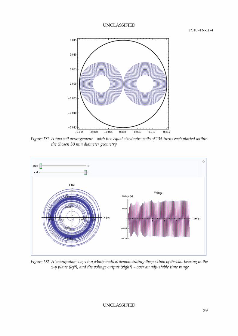
UNCLASSIFIED DSTO-TN-1174
UNCLASSIFIED 39
Figure D1 A two coil arrangement – with two equal sized wire-coils of 135 turns each plotted within the chosen 30 mm diameter geometry
Figure D2 A ‘manipulate’ object in Mathematica, demonstrating the position of the ball-bearing in the x-y plane (left), and the voltage output (right) – over an adjustable time range
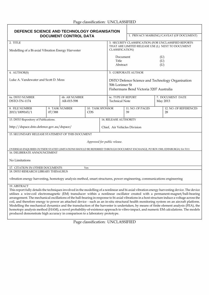
Page classification: UNCLASSIFIED
DEFENCE SCIENCE AND TECHNOLOGY ORGANISATION
DOCUMENT CONTROL DATA 1. PRIVACY MARKING/CAVEAT (OF DOCUMENT)
2. TITLE Modelling of a Bi-axial Vibration Energy Harvester
3. SECURITY CLASSIFICATION (FOR UNCLASSIFIED REPORTS THAT ARE LIMITED RELEASE USE (L) NEXT TO DOCUMENT CLASSIFICATION) Document (U) Title (U) Abstract (U)
4. AUTHOR(S) Luke A. Vandewater and Scott D. Moss
5. CORPORATE AUTHOR DSTO Defence Science and Technology Organisation 506 Lorimer St Fishermans Bend Victoria 3207 Australia
6a. DSTO NUMBER DSTO-TN-1174
6b. AR NUMBER AR-015-598
6c. TYPE OF REPORT Technical Note
7. DOCUMENT DATE May 2013
8. FILE NUMBER 2013/1009165/1
9. TASK NUMBER 07/388
10. TASK SPONSOR CDS
11. NO. OF PAGES 39
12. NO. OF REFERENCES 28
13. DSTO Repository of Publications. http://dspace.dsto.defence.gov.au/dspace/
14. RELEASE AUTHORITY Chief, Air Vehicles Division
15. SECONDARY RELEASE STATEMENT OF THIS DOCUMENT
Approved for public release. OVERSEAS ENQUIRIES OUTSIDE STATED LIMITATIONS SHOULD BE REFERRED THROUGH DOCUMENT EXCHANGE, PO BOX 1500, EDINBURGH, SA 5111 16. DELIBERATE ANNOUNCEMENT No Limitations 17. CITATION IN OTHER DOCUMENTS Yes 18. DSTO RESEARCH LIBRARY THESAURUS vibration energy harvesting, homotopy analysis method, smart structures, power engineering, communications engineering 19. ABSTRACT This report fully details the techniques involved in the modelling of a nonlinear and bi-axial vibration energy harvesting device. The device utilises a wire-coil electromagnetic (EM) transducer within a nonlinear oscillator created with a permanent-magnet/ball-bearing arrangement. The mechanical oscillations of the ball-bearing in response to bi-axial vibrations in a host structure induce a voltage across the coil, and therefore energy to power an attached device - such as an in-situ structural health monitoring system on an aircraft platform. Modelling the mechanical dynamics and the transduction of the harvester is undertaken, by means of finite element analysis (FEA), the homotopy analysis method (HAM), a novel probability-of-existence approach to vibro-impact, and numeric EM calculations. The models produced demonstrate high accuracy in comparison to a laboratory prototype.
Page classification: UNCLASSIFIED