modelling of default risk: an overview - financerisks.com default risk.pdf · modelling of default...

Modelling of Default Risk:An Overview∗

Monique JeanblancEquipe d’Analyse et Probabilites, Universite d’Evry Val d’Essonne

Boulevard des Coquibus, 91025 Evry Cedex, [email protected]

Marek RutkowskiFaculty of Mathematics and Information Science

Warsaw University of Technology00-661 Warszawa, [email protected]

October 27, 1999

Abstract

The aim of these notes is to provide a relatively concise - but still self-contained - overview ofmathematical notions and results which underpin the valuation of defaultable claims. Thoughthe default risk modelling was extensively studied in numerous recent papers, it seems nonethe-less that some of these papers lack a sound theoretical background. Our goal is to furnishresults which cover both the classic value-of-the-firm (or structural) approach, as well as themore recent intensity-based methodology. For a more detailed account of mathematical resultsrelated to the modelling of default risk, the interested reader is referred to the companion workby M. Jeanblanc and M. Rutkowski: Modelling of Default Risk: Mathematical Tools.

∗Published in: Mathematical Finance: Theory and Practice, Jiongmin Yong and Rama Cont, eds., Higher Educa-tion Press, Beijing, 2000, pp.171–269.

1

2 Default Risk: An Overview

Contents

1 Introduction 4

2 Preliminaries 4

3 Structural Approach 7

3.1 Hitting Times of a Constant Barrier . . . . . . . . . . . . . . . . . . . . . . . . . . . 8

3.1.1 Standard Brownian Motion . . . . . . . . . . . . . . . . . . . . . . . . . . . . 8

3.1.2 Brownian Motion with Drift . . . . . . . . . . . . . . . . . . . . . . . . . . . . 8

3.1.3 Geometric Brownian Motion . . . . . . . . . . . . . . . . . . . . . . . . . . . 9

3.1.4 Deterministic Volatility . . . . . . . . . . . . . . . . . . . . . . . . . . . . . . 9

3.1.5 Ornstein-Uhlenbeck Process . . . . . . . . . . . . . . . . . . . . . . . . . . . . 9

3.1.6 Bessel Processes . . . . . . . . . . . . . . . . . . . . . . . . . . . . . . . . . . 9

3.1.7 Time-homogeneous Diffusion . . . . . . . . . . . . . . . . . . . . . . . . . . . 10

3.1.8 Non-constant Barrier . . . . . . . . . . . . . . . . . . . . . . . . . . . . . . . . 11

3.2 Stochastic Barrier . . . . . . . . . . . . . . . . . . . . . . . . . . . . . . . . . . . . . 11

3.3 Jump-diffusion . . . . . . . . . . . . . . . . . . . . . . . . . . . . . . . . . . . . . . . 12

3.4 Hedging . . . . . . . . . . . . . . . . . . . . . . . . . . . . . . . . . . . . . . . . . . . 12

3.5 Term Structure Models . . . . . . . . . . . . . . . . . . . . . . . . . . . . . . . . . . 12

4 Intensity-based Approach 12

4.1 Stochastic Intensity: Classic Approach . . . . . . . . . . . . . . . . . . . . . . . . . . 13

4.1.1 Conditional Expectation . . . . . . . . . . . . . . . . . . . . . . . . . . . . . . 13

4.1.2 Hypothesis (D) . . . . . . . . . . . . . . . . . . . . . . . . . . . . . . . . . . . 14

4.2 Cox Processes and Extensions . . . . . . . . . . . . . . . . . . . . . . . . . . . . . . . 15

4.2.1 Elementary Case . . . . . . . . . . . . . . . . . . . . . . . . . . . . . . . . . . 15

4.2.2 Construction of Cox Processes . . . . . . . . . . . . . . . . . . . . . . . . . . 16

4.2.3 Conditional Expectations . . . . . . . . . . . . . . . . . . . . . . . . . . . . . 16

4.2.4 Conditional Expectation of F∞-Measurable Random Variables . . . . . . . . 18

4.2.5 Defaultable Zero-Coupon Bond . . . . . . . . . . . . . . . . . . . . . . . . . . 18

5 Hazard Functions of a Random Time 19

5.1 Conditional Expectations w.r.t. the Natural Filtration . . . . . . . . . . . . . . . . . 20

5.2 Applications to the Valuation of Defaultable Claims . . . . . . . . . . . . . . . . . . 21

5.3 Martingale Property of a Continuous Hazard Function . . . . . . . . . . . . . . . . . 22

5.4 Representation Theorem I . . . . . . . . . . . . . . . . . . . . . . . . . . . . . . . . . 25

5.5 Martingale Characterization of the Hazard Function . . . . . . . . . . . . . . . . . . 26

5.6 Duffie and Lando’s Result . . . . . . . . . . . . . . . . . . . . . . . . . . . . . . . . . 28

5.7 Generalizations . . . . . . . . . . . . . . . . . . . . . . . . . . . . . . . . . . . . . . . 29

5.7.1 Successive default times . . . . . . . . . . . . . . . . . . . . . . . . . . . . . . 29

5.7.2 Partial observations . . . . . . . . . . . . . . . . . . . . . . . . . . . . . . . . 29

M.Jeanblanc & M.Rutkowski 3

6 Hazard Processes of a Random Time 30

6.1 Conditional Expectations w.r.t. an Arbitrary Filtration . . . . . . . . . . . . . . . . 30

6.1.1 Hazard Process Γ . . . . . . . . . . . . . . . . . . . . . . . . . . . . . . . . . . 30

6.1.2 Evaluation of the Conditional Expectation E( 11 τ>tY | Gt) . . . . . . . . . . 30

6.1.3 Applications to Defaultable Bonds . . . . . . . . . . . . . . . . . . . . . . . . 31

6.1.4 Evaluation of the Conditional Expectation E(Y | Gt) . . . . . . . . . . . . . . 31

6.1.5 Martingales Associated with the Hazard Process Γ . . . . . . . . . . . . . . . 32

6.1.6 F-Intensity of a Random Time . . . . . . . . . . . . . . . . . . . . . . . . . . 33

6.2 Hypothesis (H) and Extensions . . . . . . . . . . . . . . . . . . . . . . . . . . . . . . 34

6.2.1 Hypothesis (H) . . . . . . . . . . . . . . . . . . . . . . . . . . . . . . . . . . . 34

6.2.2 Representation Theorem II . . . . . . . . . . . . . . . . . . . . . . . . . . . . 35

6.3 Martingale Hazard Process Λ . . . . . . . . . . . . . . . . . . . . . . . . . . . . . . . 35

6.3.1 Representation Theorem III . . . . . . . . . . . . . . . . . . . . . . . . . . . . 36

6.3.2 F-compensator of F . . . . . . . . . . . . . . . . . . . . . . . . . . . . . . . . 37

6.3.3 Value of a Rebate . . . . . . . . . . . . . . . . . . . . . . . . . . . . . . . . . 40

6.4 Brownian Motion Case . . . . . . . . . . . . . . . . . . . . . . . . . . . . . . . . . . . 40

6.4.1 Representation Theorem IV . . . . . . . . . . . . . . . . . . . . . . . . . . . . 40

6.4.2 Relationship Between Hypotheses (G) and (H) . . . . . . . . . . . . . . . . . 41

6.5 Uniqueness of a Martingale Hazard Process Λ . . . . . . . . . . . . . . . . . . . . . . 42

6.6 Relationship Between Hazard Processes Γ and Λ . . . . . . . . . . . . . . . . . . . . 42

7 Case of τ Measurable with Respect to F∞ 43

7.1 Notation and Basic Results . . . . . . . . . . . . . . . . . . . . . . . . . . . . . . . . 44

7.1.1 Valuation of Defaultable Claims . . . . . . . . . . . . . . . . . . . . . . . . . 45

7.1.2 Scale Function . . . . . . . . . . . . . . . . . . . . . . . . . . . . . . . . . . . 45

7.2 Last Passage Time of a Transient Diffusion . . . . . . . . . . . . . . . . . . . . . . . 46

7.2.1 F-compensator of D . . . . . . . . . . . . . . . . . . . . . . . . . . . . . . . . 46

7.2.2 Application to the Valuation of Defaultable Claims . . . . . . . . . . . . . . . 46

7.3 Last Passage Time Before Bankruptcy . . . . . . . . . . . . . . . . . . . . . . . . . . 47

7.4 Last Passage Time Before Maturity . . . . . . . . . . . . . . . . . . . . . . . . . . . . 47

7.4.1 Brownian Motion Case . . . . . . . . . . . . . . . . . . . . . . . . . . . . . . . 48

7.4.2 Brownian Motion with Drift . . . . . . . . . . . . . . . . . . . . . . . . . . . . 50

7.5 Absolutely Continuous Intensity . . . . . . . . . . . . . . . . . . . . . . . . . . . . . 52

7.6 Information . . . . . . . . . . . . . . . . . . . . . . . . . . . . . . . . . . . . . . . . . 53

7.7 Representation Theorem V . . . . . . . . . . . . . . . . . . . . . . . . . . . . . . . . 53

8 Standard Construction of a Random Time 53


1 Introduction

The aim of these notes is to provide a relatively concise - but still self-contained - overview ofmathematical notions and results which underpin the valuation of defaultable claims. Though thedefault risk modelling was extensively studied in numerous recent papers, it seems nonetheless thatsome of these papers lack a sound theoretical background. Our goal is to furnish results which coverboth the classic value-of-the-firm (or structural) approach, as well as the more recent intensity-basedmethodology.

The notes are organized as follows. In Section 2, we provide a brief introduction to the defaultrisk modelling, and to the associated mathematical concepts. Section 3 in entirely devoted to anexposition of various structural models, in which the default event is related to a hitting time to aconstant or variable barrier. In Section 4, we provide a brief overview of various models which arederived within the so-called intensity-based approach.

Subsequently, in Section 5, we provide a detailed analysis of the relatively simple case when theflow of informations available to an agent reduces to the observations of the random time whichmodels the default event. The focus is on the evaluation of conditional expectations with respect tothe filtration generated by a default time with the use of the intensity function. Results of Section5 are then generalized in Section 6 to the case when an additional information flow - formallyrepresented by some filtration F - is present. At the intuitive level, F is generated by prices of someassets, or by other economic factors (e.g., interest rates). Though in typical examples F is chosento be the Brownian filtration, most theoretical results obtained in Section 6 do not rely on such aspecification of the filtration F. Special attention is paid here to the hypothesis (H), which postulatesthe invariance of the martingale property with respect to the enlargement of F by the observationsof a default time.

In Section 7, we examine several non-trivial examples of the calculation of the stochastic intensityof a default time (or rather of the dual predictable projection of the associated first jump process).Since in this section the underlying filtration F is assumed to be generated by a Brownian motion,and it is well known that all stopping time with respect to the Brownian filtration are predictable(so that they do not admit intensity with respect to F), it is natural to examine random times whichare not F-stopping times. To be more specific, we study last passage times of a Brownian motion(with or without drift), and more general, of a diffusion process. Finally, in Section 8, we describea standard construction of a random time with a given stochastic intensity.

2 Preliminaries

In an arbitrage-free complete financial market, the t-time price Xt of a promised payoff X paid ata terminal time T is

Xt = E(X exp

(−

∫ T

t

ru du) ∣∣∣Ft),

where (rs, s ≥ 0) is the spot interest rate. In the formula above, the expectation is computed underthe so-called equivalent martingale measure (e.m.m.) which, under some technical hypotheses, isunique, and Ft is the information available at time t. The proof of this result relies on a replicationtool: with an initial investment equal to x = X0, a financial agent is able to buy a self-financingportfolio with terminal value equal to X , i.e., a hedging portfolio, and the t-time value of thisportfolio is Xt. If the market is not complete, there exist contingent claims that cannot be hedged.Let us stress that it is important to explicitly specify the information available to the agent.

In the default risk framework, a default appears at some random time τ . Let us denote by11T<τ the indicator function of the set T < τ, equal to 1 if the default occurs after T andequal to 0 otherwise. A default free contingent claim consists of a nonnegative random variablewhich represent the amount of cash paid at a prespecified time T to the owner of the claim. For a


defaultable contingent claim, the promised payment is actually done only if the default did not occurbefore maturity. If the default occurs before maturity, the payment is not done, and the defaultableclaim is worthless after default time. More generally, the payment of a defaultable claim consists oftwo parts:1) Given a maturity date T > 0, a random variable X , which does not depend on τ represents thepromised payoff – that is, the amount of cash the owner of the claim will receive at time T , providedthat the default has not occured before the maturity date T .2) A predictable process h, prespecified in the default-free world, models the payoff which is receivedif default occurs before maturity. This process is called the recovery process or the rebate.

The value of the defaultable claim is, provided that the default has not occured before time t,

Xt = E(X11T<τ exp

(−

∫ T

t

ru du)

+ hτ11τ≤T exp(−

∫ τ

t

ru du) ∣∣∣Gt),

where Gt is the information at time t. We assume that the agent knows when the default appears.At time t, the agent knows if the default has occured before; if the default has not yet occured, hehas no information on the time when it will happen.

The problem of modelling a default time is well represented in the literature. There are twomain approaches: either the default time τ is a stopping time in the asset’s filtration, or it is astopping time in a larger filtration. The papers of Cooper and Martin [13] and Rogers [52] containa comparative study of these approaches. The main difference between the two methods is that inthe first approach the default time is “announced,” whereas it is not the case in the second case.

In the first approach, the so-called structural approach, pioneered by Merton [47], the defaulttime τ is a stopping time in the filtration of the prices. Therefore the valuing of the defaultableclaim reduces to the problem of the pricing of the claim X11T<τ which is measurable with respectto the filtration of the prices at time T . This is a standard, though difficult, problem, which reduces- in a complete market case - to the computation of the expectation of the discounted payoff underthe risk-neutral probability measure.

In the second method, known as the intensity-based approach, the aim is also to compute the valueof the defaultable claim X11T<τ; however it may happen that this claim is not measurable withrespect to the σ-algebra generated by prices up to time T . In this case, it is generally assumed thatthe market is complete for the large filtration, which means that the defaultable claim is hedgeable.In order to compute the expectation of X11T<τ under the risk-neutral probability, it is convenientto introduce the notion of intensity of the default. Then, under some assumptions, the intensity ofthe default time acts as a change of the spot interest rate in the pricing formula.

We proceed somewhat differently, namely, our goal is to examine the connection between thedefault-free world and the defaultable one. We recall some well known - though perhaps forgotten -tools to compute this expectation, which simplify most of the proofs in existing literature on defaultrisk modelling. We also try to understand better the meaning of “the information of the agent”and to make precise the relation between the default time and the price’s filtration by means of thehazard process.

First, we recall that if the information is only the time when the default appears, the computationof the expectation of a defaultable payoff involves the hazard function of τ . In this case, thecompensator of the default processDt = 11τ≤t can be explicitly expressed in terms of the cumulativedistribution function of τ . We discuss a result of Duffie and Lando [21] and we give a shorter proofof this result (as well as a simpler form of the intensity of the hitting time).

Subsequently, we assume that the information of the agent at time t consists of knowledge of thebehaviour of the prices up to time t as well as the default time. We show that in this case the resultsdepend strongly on the dependence between the asset process and the default time. In particular,we show that the intensity does not provide a sufficient information as far as this link is concerned.We use some tools from the theory of enlargement of filtrations in order to compute the compensatorof N , provided that it exists. Finally, we give some examples where the usual assumptions made in


the literature are not satisfied and where the value of a default claim is not obtained by a change ofspot rate.

These notes are partially based on the recent working papers by Elliott, Jeanblanc and Yor[24] and Rutkowski [53]. Monique Jeanblanc thanks the participants to Aspet’s, INRIA’s and Ulmworkshops for stimulating discussions, as well as the organizers and participants to ISFMA SummerSchool in Shanghai. Henri Pages made a careful reading of a first version and corrected a lot ofmisprints. The remaining errors are ours.

• Some notation

We shall write F to denote a filtration (Ft, t ≥ 0). A process is said to be cadlag1 (resp. caglad) if ithas right continuous paths with left limits (left continuous paths with right limits). If X is a cadlagprocess, we denote by Xt− the limit of Xs when s goes to t, and s < t, and by ∆Xt = Xt−Xt− thejump of X at time t.

The predictable σ-algebra P on (R+ ×Ω,B × F∞) is the smallest σ-algebra making all adaptedcaglad processes measurable. This σ-algebra is generated by the processes of the form 11]a,b]Fa,where Fa ∈ Fa. In particular, any caglad adapted process is manifestly predictable.

A semi-martingale is a process X which admits the decomposition X = M + A, where M is amartingale and A stands for a predictable process with bounded variation.

The indicator function of the set B is denoted by 11B.

• Background on stopping times

We recall few basic definitions related to stopping times. The notion of a stopping time depends onthe choice of the filtration. Let (Ω,F ,F,P) be a probability space with a filtration F = (Ft)t≥0.An R+ ∪ +∞ valued random variable τ is a F-stopping time if τ ≤ t ∈ Ft for any t. Obviously,if G is a filtration larger than F, i.e., Ft ⊂ Gt for any t, and τ is a F-stopping time, then τ is a G-stopping time. A stopping time τ is F-predictable if there exists an increasing sequence of F-stoppingtimes τn such that τn < τ on τ > 0 and lim τn = τ . A stopping time τ is F-totally inaccessible iffor any F-predictable stopping time S we have

Pω ∈ Ω : τ(ω) = S(ω) <∞ = 0.

In a Brownian filtration, it can be proved that any stopping time is a predictable stopping time.The most important example of totally inaccessible stopping time is the first time when a Poissonprocess jumps.

If τ is a nonnegative random variable on some probability space (Ω,G,P) it is possible to endowΩ with a filtration such that τ is a stopping time. This filtration is not unique, and the smallestfiltration satisfying this property is Dt = σ(τ ≤ u : u ≤ t) = σ(σ(τ) ∩ τ ≤ t).• Background on stochastic calculus

Let us recall few basic facts on stochastic processes, which we shall use in what follows. A moredetailed account can be found, for instance, in Dellacherie and Meyer [18] or Protter [49].

The Doob-Meyer decomposition theorem states that, under suitable integrability assumptions,any supermartingale Z admits a decomposition Z = M − A, where M is a local martingale and Aan increasing predictable process, with A0 = 0.

A standard Poisson process (with constant intensity λ) is defined as Nt =∑∞

n=1 11Tn≤t, whereTi are random variables such that T0 = 0 and (Ti − Ti−1, i ≥ 1) are i.i.d. random variables withexponential law of parameter λt. In this case, Nt is a random variable with Poisson law of parameterλ. It is well known that the process N is a process with independent and stationary increments and

1This is a French acronym for continu a droite, limites a gauche


that Mt := Nt−λt is a martingale in its canonical filtration (see Bremaud [9] for more details). Thestochastic integral with respect to a Poisson process is easily defined as∫ t

0

ψsdNs =∑

n,Tn≤tψTn .

More generally, the process (Nt, t ≥ 0) is a (generalized) Poisson process of intensity (λt, t ≥ 0)if: (i) N is a cadlag process, constant between two jumps, with jumps of size 1, i.e. ∆Ns = Ns−Ns−equals 0 or 1, (ii) (Mt := Nt −

∫ t0 λs ds , t ≥ 0) is a martingale. Here, λ is a nonnegative process.

Then, if the process ψ is bounded and predictable, the process∫ t

0

ψs dMs =∫ t

0

ψs dNs −∫ t

0

ψsλs ds =∑

n,Tn≤tψTn −

∫ t

0

ψsλs ds

is a martingale. In particular,

E(∫ t

0

ψs dNs

)= E

(∫ t

0

ψsλs ds).

Let X and Y be two semimartingales. The integration by parts formula reads

XtYt = X0Y0 +∫

]0,t]

Xs−dYs +∫

]0,t]

Ys−dXs + [X,Y ]t,

where [X,Y ] is the quadratic covariation (the bracket) of the processes X and Y . Let us recall thatthe quadratic covariation of a continuous process and a pure jump process is equal to 0, and thatthe quadratic covariation of two pure jump processes is the sum of products of their jumps:

[N1, N2]t =∑s≤t

∆(N1)s∆(N2)s,

where ∆(Ni)s = (Ni)s − (Ni)s−. The bracket of a Brownian motion and a (generalized) Poissonprocess N is equal to 0, and the bracket of N is [N , N ]t = Nt.

3 Structural Approach

As already mentioned, there are two basic approaches to modelling default risk. In the first approach– pioneered by Black and Scholes [5] and Merton [47] – the default occurs when the assets of the firmare insufficient to meet payments on debt. If B is the debt value, the payment is max (0, VT − B),and thus we essentially deal with the same problem as in the options pricing theory.

In another approach the firm defaults when its value falls below a prespecifed level. In thiscase, the default time τ is supposed to be a stopping time in the asset’s filtration. The valuationof a defaultable claim reduces here to the problem of the pricing of the claim X11T<τ which ismeasurable with respect to the filtration of the prices at time T . Main papers to be quoted here are:Briys and de Varenne [10], Ericsson and Reneby [26], Wang [61]. Some authors investigate also theconsequences of the renegotiation of the debt: Decamps and Faure-Grimaud [14], Mella-Barral [46].

The valuation of the defaultable claim within the structural approach is a standard (but difficult)problem; it requires the knowledge of the law of the pair (τ,X). We recall here some of the mainmathematical results in this area.


3.1 Hitting Times of a Constant Barrier

Let V be a process starting at v. For any a ≥ v we introduce the first time where this processreaches a, i.e., τa(V ) = inf t ≥ 0 : Vt ≥ a. The probability law of τa(V ), or at least its Laplacetransform, can be explicitly computed in some cases. The value of a defaultable claim on h(VT )is E(h(VT )11T<τa(V )). Its evaluation requires the knowledge of the probability law of the pair(VT , τa(V )) under the e.m.m. The same studies can be done for a < v, if we set

τ−a (V ) = inft ≥ 0 : Vt ≤ a = τ−a(−V ) .

3.1.1 Standard Brownian Motion

Let V be a standard Brownian motion starting at v, that is, Vt = v + Wt. In this case, the twoevents τa(V ) ≤ t and sups≤tWs ≥ α, where α = a − v are equal. The reflection principleimplies that the r.v. sups≤tWs is equal in law to the r.v. |Wt | . Therefore,

P(τα(W ) ≤ t) = P(sups≤t

Ws ≥ α) = P( |Wt | ≥ α) = P(W 2t ≥ α2) = P(tG2 ≥ α2)

where G is a Gaussian variable, with mean 0 and variance 1. It follows that τα(W ) law=α2

G2, and the

probability density function of τa(V ) is

f(t) =a− v√2πt3

exp(− (v − a)2

2t

).

The computation of

E(11T<τa(V )h(VT )

)= E

(h(VT )

)−E(11T≥τa(V )h(VT )

)can be done using Markov property:

E(11T≥τa(V )h(VT )

)= E

(11T≥τa(V )E(h(VT ) | Fτa(V ))

)= E

(11T≥τa(V ) h(WT−τa(V ) + a)

)=

∫ T

0

du f(u)E(h(WT−u + a)

),

where W is a Brownian motion independent of τa(V ), with W0 = 0.

3.1.2 Brownian Motion with Drift

Suppose that Vt = v+µt+σWt, with σ > 0. Then, τa(V ) ≤ t = τα(V ) ≤ t, where Vt =µt

σ+Wt

and α = (a− v)/σ. From Girsanov’s theorem, we can deduce the law of τa(V ). Indeed, if we denotefor simplicity τα = τα(W ), then

P(τα(V ) ≥ t) = E(11τα≥t exp

(µσWτα −

12µ2

σ2τα

))= exp

(µσα)E

(11τα≥t exp

(− 12µ2

σ2τα

))and the quantity

E(11τα≥t exp

(− 12µ2

σ2τα

))can be computed from the density of τα. Indeed, tedious computations lead to

E(11τα<s e− ν2

2 τα) = H(ν, |α | , s)


whereH(ν, x, s) = e−νxN (

ν − x√s

)+ eνxN (− ν − x√

s

)(1)

and N stands for the cumulative distribution function of the standard Gaussian law. The densityof τα(V ) is

P0(τα(V ) ∈ dt) =|α|√2πt3

exp− (α− µt)2

2t,

where µ = µ/σ (see Borodin and Salminen [7], p. 223, formula 2.0.2).

3.1.3 Geometric Brownian Motion

If V is a geometric Brownian motion such that

dVt = Vt(µdt+ σ dWt)

then for a > v > 0 we have

τa(V ) = inft ≥ 0 : v exp

((µ− σ2

2)t+ σWt

) ≥ a

= inft ≥ 0 :

(µ− σ2

2)t+ σWt ≥ ln

a

v

so that the problem reduces to the case of a Brownian motion with drift.

3.1.4 Deterministic Volatility

If dVt = σ(t) dWt, where W is a Brownian motion and σ is a deterministic function, a change oftime will give the answer. In fact, from the Dambis-Dubins-Schwarz theorem, the martingale Vis a changed time Brownian motion. More precisely, there exists a Brownian motion W such thatVt = WA(t) where A(t) = 〈V, V 〉t =

∫ t0 σ

2(s) ds. Using this change of time, and the equality

τa(V ) < t = sups≤t

Vs > a = sups≤t

WA(s) > a = τa(W ) < A(t)

we get the result. To the best of our knowledge, no closed-form expression is known for the probabilitylaw of the hitting time when V satisfies dVt = µdt+ σ(t) dWt.

3.1.5 Ornstein-Uhlenbeck Process

Let (rt, t ≥ 0) be defined as

drt = (φ − λrt) dt+√β dWt, r0 = r,

and τρ = inf t ≥ 0 : rt ≥ ρ. For any ρ > r, the density function of τρ equals

f(t) =ρ− r0√2βπt3

(λt

sinhλt

)3/2

eλt/2 exp[− λ

2β

((ρ− φ

λ

)2 − (r0 − φ

λ

)2 + (ρ− r0)2 cothλt)].

For the derivation of the last formula, the reader is referred to Leblanc’s thesis [40] (where there aresome misprints in the result, however).

3.1.6 Bessel Processes

A Bessel process R with index ν ≥ 0 (or with dimension δ with ν =δ

2− 1) is a diffusion process

which takes values in R+, and has the infinitesimal generator

Aν =12d2

dx2+

2ν + 12x

d

dx.


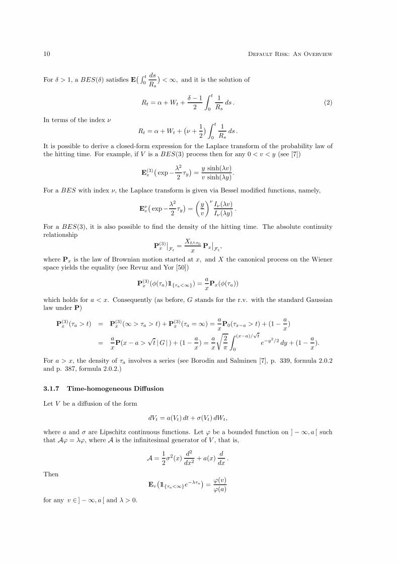
For δ > 1, a BES(δ) satisfies E( ∫ t

0

ds

Rs

)<∞, and it is the solution of

Rt = α+Wt +δ − 1

2

∫ t

0

1Rs

ds . (2)

In terms of the index ν

Rt = α+Wt +(ν +

12) ∫ t

0

1Rs

ds .

It is possible to derive a closed-form expression for the Laplace transform of the probability law ofthe hitting time. For example, if V is a BES(3) process then for any 0 < v < y (see [7])

E(3)v

(exp−λ

2

2τy

)=y sinh(λv)v sinh(λy)

.

For a BES with index ν, the Laplace transform is given via Bessel modified functions, namely,

Eνv

(exp−λ

2

2τy

)=

(y

v

)νIν(λv)Iν(λy)

.

For a BES(3), it is also possible to find the density of the hitting time. The absolute continuityrelationship

P(3)x

∣∣Ft

=Xt∧τ0x

Px

∣∣Ft,

where Px is the law of Brownian motion started at x, and X the canonical process on the Wienerspace yields the equality (see Revuz and Yor [50])

P(3)x (φ(τa)11τa<∞) =

a

xPx(φ(τa))

which holds for a < x. Consequently (as before, G stands for the r.v. with the standard Gaussianlaw under P)

P(3)x (τa > t) = P(3)

x (∞ > τa > t) + P(3)x (τa = ∞) =

a

xP0(τx−a > t) + (1− a

x)

=a

xP(x− a >

√t |G | ) + (1− a

x) =

a

x

√2π

∫ (x−a)/√t

0

e−y2/2 dy + (1− a

x).

For a > x, the density of τa involves a series (see Borodin and Salminen [7], p. 339, formula 2.0.2and p. 387, formula 2.0.2.)

3.1.7 Time-homogeneous Diffusion

Let V be a diffusion of the form

dVt = a(Vt) dt+ σ(Vt) dWt,

where a and σ are Lipschitz continuous functions. Let ϕ be a bounded function on ] −∞, a [ suchthat Aϕ = λϕ, where A is the infinitesimal generator of V , that is,

A =12σ2(x)

d2

dx2+ a(x)

d

dx.

Then

Ev

(11τa<∞e

−λτa)

=ϕ(v)ϕ(a)

for any v ∈ ]−∞, a [ and λ > 0.


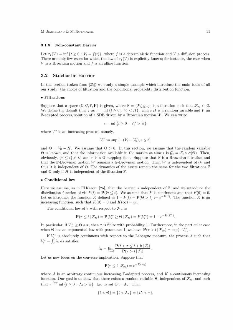
3.1.8 Non-constant Barrier

Let τf (V ) = inf t ≥ 0 : Vt = f(t), where f is a deterministic function and V a diffusion process.There are only few cases for which the law of τf (V ) is explicitly known; for instance, the case whenV is a Brownian motion and f is an affine function.

3.2 Stochastic Barrier

In this section (taken from [25]) we study a simple example which introduce the main tools of allour study: the choice of filtration and the conditional probability distribution function.

• Filtrations

Suppose that a space (Ω,G,F,P) is given, where F = (Ft)t≥0 is a filtration such that F∞ ⊂ G.We define the default time τ as τ = inf t ≥ 0 : Vt < H, where H is a random variable and V anF-adapted process, solution of a SDE driven by a Brownian motion W . We can write

τ = inf t ≥ 0 : V ∗t > Θ,where V ∗ is an increasing process, namely,

V ∗t := sup −(Vs − V0), s ≤ tand Θ = V0 − H . We assume that Θ > 0. In this section, we assume that the random variableΘ is known, and that the information available in the market at time t is Gt = Ft ∨ σ(Θ). Then,obviously, τ ≤ t ∈ Gt and τ is a G-stopping time. Suppose that F is a Brownian filtration andthat the F-Brownian motion W remains a G-Brownian motion. Then W is independent of G0 andthus it is independent of Θ. The dynamics of the assets remain the same for the two filtrations F

and G only if H is independent of the filtration F.

• Conditional law

Here we assume, as in El Karoui [25], that the barrier is independent of F, and we introduce thedistribution function of Θ: F (t) = P(Θ ≤ t). We assume that F is continuous and that F (0) = 0.Let us introduce the function K defined as 1 − F (t) = P(Θ > t) := e−K(t). The function K is anincreasing function, such that K(0) = 0 and K(∞) = ∞.

The conditional law of τ with respect to F∞ is

P(τ ≤ t | F∞) = P(V ∗t ≥ Θ | F∞) = F (V ∗t ) = 1− e−K(V ∗t ).

In particular, if V ∗∞ ≥ Θ a.s., then τ is finite with probability 1. Furthermore, in the particular casewhen Θ has an exponential law with parameter 1, we have P(τ > t | F∞) = exp(−V ∗t ).

If V ∗t is absolutely continuous with respect to the Lebesgue measure, the process λ such thatV ∗t =

∫ t0λs ds satisfies

λt = limh→0

P(t < τ ≤ t+ h | Ft)P(τ > t | Ft) .

Let us now focus on the converse implication. Suppose that

P(τ ≤ t | F∞) = e−K(At)

where A is an arbitrary continuous increasing F-adapted process, and K a continuous increasingfunction. Our goal is to show that there exists a random variable Θ, independent of F∞, and suchthat τ law= inf t ≥ 0 : Λt > Θ. Let us set Θ := Λτ . Then

t < Θ = t < Λτ = Ct < τ,


where C is the right inverse of Λ, so that ΛCt = t. Therefore

P(Θ > t | F∞) = e−K(ΛCt ) = e−K(t).

We have thus established the required properties, namely, the probability law of Θ and its indepen-dence of the σ-field F∞.

3.3 Jump-diffusion

Zhou [65] studies the case when the value of the firm is modelled via a jump-diffusion process onthe form

dVt = Vt−((µ− λν) dt + σ dWt + Φt dN∗

t

), V0 = v,

where W is a Brownian motion, N∗ is a Poisson process, and Φ represents the jump amplitude.The processes W,N∗ and Φ are assumed to be mutually independent. The default time is modelledas the first time when the process V falls below the level a. Zhou computes the expectation of thediscounted payoff under the risk neutral measure, assuming that the risk premium associated withthe jump is equal to zero. A closed-form expression for the probability law of the pair (VT , τ) is notknown in this case. The difficulty is that the level may be crossed either in a continuous way or witha jump. Zhou gives an approximation of the expectation, using a certain time discretization of theprocess V . If Φ is a nonnegative constant and v > a, we have Vτ = a, and the Laplace transform ofτ can be easily found.

3.4 Hedging

The defaultable contingent claim 11T<τh(VT ) is an FT -measurable random variable. If the default-free market is complete, this remains true for the defaultable market and it is possible to hedge anydefaultable contingent claim. This is not the case in Zhou’s model, however.

3.5 Term Structure Models

A substantial literature proposes to model both the default free term structure and the term structurerepresenting the relative prices of different maturities of default-risky debt, using an extension of themethod developed by Heath-Jarrow-Morton. Major papers in this area include Jarrow and Turnbull[31], Schonbucher [56, 55], Hubner [29, 28], and Bielecki and Rutkowski [3].

4 Intensity-based Approach

From now on, we shall focus our attention on the intensity-based valuation. The default time τ isgiven as a random time, i.e., a nonnegative random variable. We associate with this random timethe counting process D defined as Dt = 11τ≤t. The process D is an increasing process, cadlag,equal to 0 before the default and equal to 1 after default. Essentially, the intensity of τ is definedas the nonnegative adapted process λ such that

Mt := Dt −∫ t∧τ

0

λu du

is a martingale. This approach, more recent than the structural one, is also known as the reduced-form approach, and has been introduced by Jarrow and Turnbull [31], Jarrow, Lando and Turnbull[32], Lando [37, 38], Duffie and Singleton [19]. More recents contributions are Hubner [29, 28]Arvanatis, Gregory and Laurent [1], Schonbucher [54, 55, 56, 58] and Lotz [42, 43] among others.

As we shall see in what follows, the choice of the filtration is essential.


4.1 Stochastic Intensity: Classic Approach

In this section, we adopt the standard definition of stochastic intensity of a random time τ withrespect to a filtration J such that τ is a J-stopping time. Namely, we say that, for a given filtrationJ = (Jt)t≥0, the J-adapted nonnegative process λ is the J-intensity (or briefly, the stochasticintensity) of τ if the process Dt−

∫ τ∧t0 λs ds is a J-martingale. We emphasize that if such a definition

of a stochastic intensity of τ is adopted, then the stochastic intensity λ has virtually no meaningafter time τ .

Let us consider an elementary example. If τ is an exponentially distributed random variable onsome filtered probability space (Ω, J,P), with the parameter λ > 0, then the constant λ is referredto as the hazard rate of τ, and the stochastic intensity of τ (with respect to any sub-filtration J

such that τ is a J-stopping time) equals λt = λ11t≤τ if Dt −∫ τ∧t0

λds is a J-martingale. Such adefinition of stochastic intensity is quite sufficient in the theory of (marked) point processes2 sincein this case one is interested mainly in the filtration generated by the point process itself.

In financial applications, however, we frequently deal with some prespecified underlying filtration,3

F say, and thus it is more appropriate to introduce the more specific concept of a F-intensity of arandom time. The case of a F-intensity with respect to an external filtration F is examined inSection 6 below (see, in particular, Section 6.1.6). In fact, we find it convenient to introduce tworelated notions: of a F-hazard process Γ and a F-martingale hazard process Λ of a random time τ (seeDefinitions 6.1 and 6.2, respectively). One of our main goals is to study the relationships betweenthese two concepts, under various types of hypotheses imposed on the underlying filtrations.

Remark 4.1 Let J be a filtration larger than J, i.e., Jt ⊂ Jt for every t ≥ 0, and λ the J-intensityof D. The process D is manifestly J-adapted, and thus τ is still a stopping time with respect to theenlarged filtration J . However, it may happen that D does not admit an intensity in the filtrationJ, and if the J-intensity exists, it may be different from J-intensity.

In the remaining part of this section, we present the main results and examples which can befound in existing financial literature.

4.1.1 Conditional Expectation

Suppose that τ is a random time with J-intensity λ – that is, the process Mt = Dt −∫ t∧τ0 λsds is a

J-martingale. Let F be a subfiltration of J.

Definition 4.1 The pair (h,X) where h is a F-predictable process and X a FT -measurable nonneg-ative random variable is called a F-adapted defaultable claim. It corresponds to a terminal payoffX which is paid if the default has not appeared before or at time T, and a rebate h which is paidwhen the default appears.

Let (h,X) be a F-adapted defaultable claim with the value process S. Let

RtSt = E(Rτhτ11t<τ≤T +XRT11T<τ | Jt

)be its discounted value. We assume here that the savings account B satisfies

Bt = exp(∫ t

0

ru du)

for some F-adapted nonnegative process r (known as the short-term interest rate), and the discountfactor R equals Rt = B−1

t .

2See, for instance, Last and Brandt [39].3Typically, it is generated by the observations of price processes of primary assets.


Proposition 4.1 Let λu = λu(1 −Du). Then

RtSt = E(∫ T

t

Ruhuλudu+XRT 11T<τ | Jt)

(3)

and

RtSt = E(∫ T

t

(huλu − ruSu) du+X11T<τ | Jt). (4)

Proof. From the definition of the stochastic integral, we get

Rτhτ11t<τ≤T =∫ T

t

RuhudDu =∫ T

t

RuhudMu +∫ T

t

Ruhuλudu.

Then, the martingale property of the stochastic integral with respect to M yields

E(Rτhτ11t<τ≤T | Jt

)= E

(∫ T

t

RuhudDu | Jt)

= E(∫ T

t

Ruhuλudu | Jt).

The formula above proves that the process RtSt+∫ t0Ruλuhudu is a J-martingale. This immediately

yields (3). Furthermore, using Ito’s formula we conclude that the process St +∫ t0(λuhu − ruSu)du

is a J-martingale and this proves (4). 2

4.1.2 Hypothesis (D)

As before, τ is a random time with J-intensity λ, i.e., the process Mt = Dt −∫ t∧τ0

λsds is a J-martingale. In order to give the value of a defaultable claim in a neat form, many authors (see, e.g.,Duffie et al. [21, 22]) make the following hypothesis:

Hypothesis (D). The intensity λ admits at least one extension up to infinity, say λ∗ such thatsuch that the (right-continuous) process V, given by the formula

Vt = E(Y e

−∫ T

tλ∗u du | Jt), (5)

is continuous at τ, that is, ∆VT∧τ = VT∧τ − V(T∧τ)− = 0.

Their main result is the following:

Proposition 4.2 For a fixed T > 0, let Y be a JT -measurable random variable. Under hypothesis(D) we have, for any t < T,

E( 11 τ>T Y | Jt) = 11 τ>tE(Y e

−∫

T

tλ∗u du | Jt). (6)

Proof. We shall first check that

11 τ>tVt = E(∆Vτ 11 t<τ≤T + 11 τ>TY

∣∣Jt). (7)

From the definition, Vt = eΛ∗t Mt, where M is a J-martingale: Mt = E

(Y e−Λ∗T | Jt) for t ∈ [0, T ] ,

and Λ∗t =∫ t0 λ

∗s ds. Using Ito’s product rule, we obtain

dVt = Mt− d (eΛ∗t ) + eΛ

∗t dMt = Vt−e−Λ∗t d (eΛ

∗t ) + eΛ

∗t dMt. (8)

Define Ut = DtVt, where Dt = 11 τ>t = 1−Dt, and observe that (7) may be rewritten as follows

Ut = E(∫

]t,T ]

∆Vu dDu + 11 τ>TY∣∣∣Jt). (9)


On the other hand, an application of Ito’s product rule yields

dUt = Dt− dVt − Vt− dDt + ∆Vt∆Dt.

Combining the last formula with (8), and noticing that ∆Dt = −∆Dt, we obtain

dUt = Dt−(Vt−e−Λ∗t d (eΛ

∗t ) + eΛ

∗t dMt

)− Vt− dDt −∆Vt dDt.

After rearranging, we getdUt = −∆Vt dDt + dMt, (10)

where M stands for a J-martingale. More precisely,

dMt = Dt−eΛ∗t dMt + dM∗

t ,

wheredM∗

t = −Vt−(dDt − 11 τ≥te−Λ∗t d (eΛ

∗t )

)= −Vt− d (Dt − Λt∧τ ),

so that M∗ is a J-martingale. Since obviously UT = 11 τ>TY, (10) implies (9). If V is continuousat τ then (7) yields

E( 11 τ>T Y | Jt) = 11 τ>tE( 11τ>T Y | Jt) = 11 τ>tVt = 11 τ>tE(Y eΛ

∗t−Λ∗T | Jt).

This completes the proof. 2

Remark 4.2 It should be observed that the ‘natural’ extension λ∗u = λu11]0,τ ] does not satisfy

(D). In fact, it can be shown that the process E(e−

∫τ

tλu du | Jt) is discontinuous at τ . Moreover,

this hypothesis can not be satisfied for every Y . Indeed, it would imply that every J-martingale iscontinuous, but this is manifestly not true. Therefore, the suitable choice of the extended intensityprocess λ∗ should depend on Y .

4.2 Cox Processes and Extensions

Let (Ω,F,P) be a filtered probability space. An example of default time with stochastic intensityis a single jump Cox process, that is, a process Dt = 11t≤τ such that there exists an F-adaptedprocess f with

P(τ ≤ t | F∞) =∫ t

0

fs ds := Ft.

In this case

P(τ ≤ t | Ft) = Ft = 1− exp(−

∫ t

0

λu du),

where λs =fs

1− Fs. In order to study the intensity of τ , we have to introduce a filtration such that

τ is a stopping time; this is not the case for F. Indeed, this would imply that Ft = P(τ ≤ t | Ft) isequal to Dt, which is manifestly not true.

4.2.1 Elementary Case

In the early papers on intensity-based approach to credit risk modelling (see, for instance, [31, 37]) thedefault time is modelled as the first jump of a Poisson process, which is assumed to be independentof the assets prices and/or of the value of the firm.

Suppose that F is the filtration of the assets prices and that N is a Poisson process, independentof F, with stochastic intensity λ. We denote by τ the first time when the Poisson process has a jump,


i.e., τ = T1. By Dt = Nt∧τ we denote the associated single jump process. The canonical filtrationof D is D = (Dt, t ≥ 0), where Dt = σ(Ds, s ≤ t), and the intensity is clearly D-adapted. Finally, Gtstands for the σ-algebra generated by Ft and Dt > We shall write briefly: G = D ∨ F.

The D-martingale M , stopped at the D-stopping time τ

Mt = Mt∧τ = Dt −∫ t∧τ

0

λsds

is a D-martingale. We denote by λ a stochastic process which is equal to λ up to time τ .

It is useful to observe that the process (Mt = Dt−∫ t∧τ0

λsds , t ≥ 0) is not only a D-martingale,but also a G-martingale.4 The independence property allows us to state that any bounded F∞-measurable r.v. X we have

E(X11τ>T | Gt) = 11τ>tE(

exp(−

∫ T

t

λu du) ∣∣∣Dt)E(X | Ft).

Indeed, it suffices to recall that, if F and D are independent filtrations then for any boundedF∞-measurable r.v. X and any bounded D∞-measurable r.v. Y , we have E(XY | Ft ∨ Dt) =E(X | Ft)E(Y | Dt) for any t. Such a model is used in the literature on credit ratings, where thedefault-time is represented by the first time where a Markov-chain reaches an absorbing state (see[38]).

4.2.2 Construction of Cox Processes

Let (Ω,G,P) be a probability space, and (Xt, t ≥ 0) a continuous diffusion process on this space.We denote by F its canonical filtration, satisfying the usual conditions. A nonnegative function λis given. We assume that there exists a random variable Θ, independent of X , with an exponentiallaw: P(Θ ≥ t) = e−t. We define the random time τ as the first time when the process

∫ t0λ(Xs) ds

is above the random level Θ, i.e.,

τ = inf t ≥ 0 :∫ t

0

λ(Xs) ds ≥ Θ.

The mutual independence of Θ and X will avoid us to enter in the enlargement of filtration’s world.This will be done in a next section, in the general case, that is, when the independence hypothesisis relaxed.

Another example is to choose τ = inf t ≥ 0 : NΛt = 1, where Λt =∫ t0 λs ds and N is a Poisson

process with intensity 1, independent of the filtration F. The second method is in fact equivalent tothe first. Cox processes are used in a great number of studies (see, e.g., [38, 48]). We shall generalizethis approach in Section 8.

4.2.3 Conditional Expectations

We write Dt = 11τ≤t and Dt = σ(Ds : s ≤ t). Let us check that the above process D is a Coxprocess.

Lemma 4.1 The conditional distribution function of τ given the σ-field Ft is for t ≥ s

P(τ > s | Ft) = exp(−

∫ s

0

λ(Xu) du).

4Notice that a martingale in a given filtration is not necessarily a martingale in a larger filtration.


Proof. The proof follows from the equality τ > s = ∫ s0λ(Xu) du > Θ. From the independence

assumption and the Ft-measurability of∫ s0λ(Xu) du for s ≤ t, we obtain

P(τ > s | Ft) = P( ∫ s

0

λ(Xu)du ≥ Θ∣∣∣Ft) = exp

(−

∫ s

0

λ(Xu) du).

In particular, we haveP(τ ≤ t | Ft) = P(τ ≤ t | F∞).

Let us notice that the process Ft = P(τ ≤ t | Ft) is here an increasing process. 2

We introduce the filtration Gt = Ft ∨Dt, that is, the enlarged filtration generated by the under-lying filtration F and the process D. (We denote by F the original Filtration and by G the enlarGedone.) We shall frequently write G = F ∨ D.

It is easy to describe the events which belong to the σ-field Gt on the set τ > t. Indeed, ifGt ∈ Gt, then Gt ∩ τ > t = Bt ∩ τ > t for some event Bt ∈ Ft. Therefore any Gt-measurablerandom variable Yt satisfies 11τ>tYt = 11τ>tyt, where yt is an Ft-measurable random variable.

We emphasize that the enlarged filtration G = F∨D is here the filtration which should be takeninto account; the filtration generated by Ft and σ(Θ) is too large. In the latter filtration τ wouldbe a predictable stopping time, and would not admit an intensity.

Proposition 4.3 Let X be an integrable r.v. Then,

11τ>tE(X | Gt) = 11τ>tE(X11τ>t | Ft)E(11τ>t | Ft) .

Proof. From the remarks on the Gt-measurability, if Yt = E(X | Gt), then there exists yt, which isFt-measurable, such that

11τ>tE(X | Gt) = 11τ>tyt

and multiplying both members by the indicator function, we deduce yt =E(X11τ>t | Ft)E(11τ>t | Ft) . 2

We shall now compute the (conditional) expectation of a predictable process at time τ.

Lemma 4.2 (i) Let Λu =∫ u0λ(Xs) ds. If h is a F-predictable process then

E(hτ ) = E(∫ ∞

0

huλ(Xu) exp(− Λu) du

)E(hτ | Ft) = E

(∫ ∞

0

huλ(Xu) exp(− Λu

)du

∣∣∣Ft)and

E(hτ | Gt) = E( ∫ ∞

t

huλ(Xu) exp(Λt − Λu

)du

∣∣∣Ft)11τ>t + hτ11τ≤t. (11)

(ii) The process (Dt −∫ t∧τ0

λ(Xs)ds, t ≥ 0) is a G-martingale.

Proof. Let ht = 11]v,w](t)Bv where Bv ∈ Fv. Then,

E(hτ | Ft) = E(E(11]v,w](τ)Bv | F∞)

∣∣∣Ft) = E(Bv

(e−Λv − e−Λw

) | Ft)= E

(Bv

∫ w

v

λ(Xu)e−Λu du∣∣∣Ft)

= E(∫ ∞

0

huλ(Xu)e−Λudu∣∣∣Ft)


and the result follows from the monotone class theorem.

The martingale property (ii) follows from integration by parts formula. Let t < s. Then, on theone hand

E(Ds −Dt | Gt) = P(t < τ ≤ s | Gt) = 11t<τP(t < τ ≤ s | Ft)

P(t < τ | Ft)= 11t<τE(1− exp(Λs − Λt) | Ft).

On the other hand, from part (i)

E(∫ s∧τ

t∧τλ(Xu)du

∣∣∣Gt) = E(Λs∧τ − Λt∧τ | Gt

)= 11t<τE

(∫ ∞

t

huλue−(Λu−Λt)du

∣∣∣Ft)where hu = Λ(s ∧ u)− Λ(t ∧ u). Consequently,∫ ∞

t

huλue−(Λu−Λt)du =

∫ s

t

(Λu − Λs)λue−(Λu−Λt)du+ (Λt − Λs)∫ ∞

s

λue−(Λu−Λt)du

= −(Λs − Λt)e−(Λs−Λt) +∫ s

t

λ(u)e−(Λu−Λt)du + (Λs − Λt)e−(Λs−Λt)

= 1− e−(Λs−Λt).

This ends the proof. 2

4.2.4 Conditional Expectation of F∞-Measurable Random Variables

Lemma 4.3 Let X be an F∞-measurable r.v. X. Then

E(X11τ>t | Ft) = exp(− ∫ t

0

λ(Xs) ds)E(X | Ft),

E(X | Gt) = E(X | Ft). (12)

Proof. Let X be an F∞-measurable r.v. Then,

E(X11τ>t | Ft) = E(E(X11τ>t | F∞) | Ft) = P(τ > t | Ft)E(X | F∞).

To prove that E(X | Gt) = E(X | Ft), it suffices to check that

E(Bth(τ ∧ t)X) = E(Bth(τ ∧ t)E(X | Ft))for any Bt ∈ Ft and any h = 11[0,a]. For t ≤ a, the equality is obvious. For t > a, we have

E(Bt11τ≤aE(X | Ft)) = E(BtE(X | Ft)E(11τ≤a | F∞)) = E(E(BtX | Ft)E(11τ≤a | Ft))= E(XBtE(11τ≤a | Ft)) = E(BtX11τ≤a)

as expected. 2

Let us remark that (12) implies that every F-square integrable martingale is a G-martingale.However, equality (12) does not apply to any G-measurable random variable; in particular P(τ ≤t | Gt) = 11τ≤t is not equal to Ft = P(τ ≤ t | Ft).

4.2.5 Defaultable Zero-Coupon Bond

Similar computations to that of the preceding paragraph show that

E(11T<τ | Gt) = 11τ>tE(11T<τ | Ft)E(11τ>t | Ft) = 11τ>tE

(exp

(− ∫ T

t

λ(Xs) ds) ∣∣∣Ft).


Suppose that the price at time t of a default-free bond paying 1 at maturity t is

B(t, T ) = E(

exp(− ∫ T

t

r(Xs) ds) ∣∣∣Ft).

The value of a defaultable zero-coupon bond is

E(11T<τ exp

(− ∫ T

t

r(Xs) ds) ∣∣∣Gt) = 11τ>tE

(exp

(− ∫ T

t

[r(Xs) + λ(Xs)] ds) ∣∣∣Ft).

The t-time value of a corporate bond, which pays δ at time T in case of default and 1 otherwise, isgiven by

E(e−

∫ T

tr(Xs) ds (δ11τ≤T + 11τ>T)

∣∣∣Ft).The last quantity is equal to

δB(t, T ) + 11τ>t(1− δ)E(

exp(− ∫ T

t

[r(Xs) + λ(Xs)] ds) ∣∣∣Ft).

It can be proved that, if h is some F-predictable process then

E(hτ11τ≤T | Gt) = hτ11τ≤t + 11τ>tE( ∫ T

t

hueΛt−Λuλ(Xu)du | Ft

).

The credit risk model of this kind was studied extensively by Lando [38].

5 Hazard Functions of a Random Time

In this section, the problem of quasi-explicit evaluation of various conditional expectations is studiedin a very special case when the only filtration available in calculations is the natural filtration of arandom time. In practical terms, we consider here an individual who observes the random time, buthas no access to any other information. More general situations are examined in the next section.

We start with some well known facts established for the first time in Dellacherie [15] or [16](p.122), and used again in Chou and Meyer [11], Liptser and Shiryaev [41], Elliott [23], Dellacherieand Meyer [18] (p.237) or more recently in Rogers and Williams [51] and Cocozza-Thivent [12] amongothers.

Suppose that τ is an R+∪∞-valued random variable on some probability space (Ω,G,P) suchthat P(τ = 0) = 0 and P(τ > t) > 0, ∀t ∈ R+. As before, we denote by (Dt ; t ≥ 0) the defaultprocess, defined as the right-continuous increasing process Dt = 11τ≤t, and by D its naturalfiltration Dt = σ(Du, u ≤ t), completed as usual with P-negligeable sets. This right-continuous,complete filtration D is generated by the sets τ ≤ s for s ≤ t (that is the σ-algebra σ(t ∧ τ))and the atom τ > t and is the smallest filtration satisfying the usual hypotheses such that τ is aD-stopping time.

Notice that any Dt-measurable integrable r.v. H is of the form H = h(τ)11τ≤t+ h11τ>t whereh is a Borel function defined on [0, t] and h a constant.

Lemma 5.1 If Y is any integrable, G-measurable random variable then

E(Y | Dt) = 11τ≤tE(Y | D∞) + 11τ>tE(Y 11τ>t)P(τ > t)

. (13)

In particular,

E(Y | Dt)11τ>t = 11τ>tE(Y 11τ>t)P(τ > t)

(14)


and if Y is σ(τ)-measurable, i.e. Y = h(τ), then

E(Y | Dt) = 11τ≤tY + 11τ>tE(Y 11τ>t)P(τ > t)

= 11τ≤tY + 11τ>t1

P(τ > t)

∫]t,∞]

h(u)dP(τ ≤ u).

Proof. Let t be fixed. The r.v. E(Y | Dt) is Dt-measurable. Therefore, it can be written in the formE(Y | Dt) = h(τ)11τ≤t + A11τ>t where A is constant and h a Borel function. Multiplying bothsides by 11τ>t, and taking the expectation, we obtain

E[11τ>tE(Y | Dt)] = E[E(11τ>tY | Dt)] = E[11τ>tY ] = AP(τ > t) .

It is easy to check that, on the set τ ≤ t, we have E(Y | Dt) = h(τ) = E(Y | τ) = E(Y | D∞). Infact, we have given the right-continuous version of the martingale E(Y | Dt). 2

5.1 Conditional Expectations w.r.t. the Natural Filtration

For easy further reference, let us write down some special cases of the formulae above. For any t < swe have

P(τ > s | Dt) = 11 τ>tP(τ > s | τ > t) = 11 τ>tP(τ > s)P(τ > t)

= 11 τ>t1− F (s)1− F (t)

, (15)

where F (t) = P(τ ≤ t) be the right-continuous distribution function of τ. The following result is astraightforward consequence of (15).

Corollary 5.1 The process M which equals

Mt =1−Dt

1− F (t), ∀ t ∈ R+, (16)

follows a D-martingale. Equivalently,

E(Ds −Dt | Dt) = (1 −Dt)F (s)− F (t)

1− F (t)= 11τ>t

F (s)− F (t)1− F (t)

, ∀ t ≤ s. (17)

Proof. The equality (15) can be rewritten as follows

E(1−Ds | Dt) = (1−Dt)1− F (s)1 − F (t)

.

This immediately yields the martingale property of M. 2

Before we proceed further, let us recall the standard notion of the hazard function of τ.

Definition 5.1 The increasing function Γ : R+ → R+ given by the formula

Γ(t) = − ln (1− F (t)), ∀ t ∈ R+, (18)

is called the hazard function of τ.

It is clear that the relationship F (t) = e−Γ(t) is satisfied. If the cumulative distribution functionF is an absolutely continuous function, that is, F (t) =

∫ t0 f(u) du, for some function f : R+ → R+,

then we haveF (t) = 1− e−Γ(t) = 1− e

−∫ t

0γ(u) du

, ∀ t ∈ R+,


where γ(t) = f(t)(1 − F (t))−1. It is clear that γ : R+ → R is a nonnegative function and satisfies∫∞0 γ(u) du = ∞, since F (∞) = 1. The function γ is called the intensity function (or hazard rate)

of τ.

Using the hazard function Γ, we may rewrite (13) as follows

E(Y | Dt) = 11τ≤tE(Y | τ) + 11 τ>t eΓ(t) E( 11 τ>tY ), (19)

and (15) takes the formP(τ > s | Dt) = 11 τ>t eΓ(t)−Γ(s).

Corollary 5.2 Assume that Y is D∞-measurable, so that Y = h(τ) for some Borel measurablefunction h : R+ → R. If the hazard function Γ of τ is continuous then

E(Y | Dt) = 11τ≤th(τ) + 11 τ>t

∫ ∞

t

h(u)eΓ(t)−Γ(u) dΓ(u). (20)

In particular,

E(h(τ)) =∫ ∞

0

h(u)e−Γ(u) dΓ(u) .

If τ admits the intensity function γ then

E(Y | Dt) = 11τ≤th(τ) + 11 τ>t

∫ ∞

t

h(u)γ(u)e−∫

u

tγ(v) dv

du. (21)

In particular, for any t ≤ s we have

P(τ > s | Dt) = 11 τ>te−

∫ s

tγ(v) dv (22)

andP(t < τ < s | Dt) = 11 τ>t

(1− e

−∫

s

tγ(v)dv

). (23)

The following simple result appears to be useful.

Lemma 5.2 The process L given by the formula

Lt := 11 τ>teΓ(t) = (1−Dt)eΓ(t), ∀ t ∈ R+, (24)

follows a D-martingale.

Proof. It suffices to observe that L coincides with the process M introduced in Corollary 5.1. 2

5.2 Applications to the Valuation of Defaultable Claims

Let us fix T > 0. We assume that the continuously compounded interest rate r follows a nonnegativedeterministic function so that the price at time t of a unit default-free zero-coupon bond of maturityT equals

B(t, T ) = e−

∫T

tr(v) dv

, ∀ t ∈ [0, T ].

Our goal is to find quasi-explicit expressions for “values” of certain defaultable claims. Let us assumethat Y = 11τ≤T h(τ) + 11τ>T c, where c is a constant. If Γ is continuous then (20) yields

E(Y | Dt) = 11τ≤th(τ) + 11 τ>t( ∫ T

t

h(u)eΓ(t)−Γ(u) dΓ(u) + ceΓ(t)−Γ(T )). (25)


Similarly, for a fixed t ≤ T denote by Yt the random variable (discounted payoff at time t)

Yt = 11τ≤T h(τ)e−

∫ τ

tr(v) dv + 11 τ>T ce

−∫ T

tr(v) dv

. (26)

If Γ is an absolutely continuous function, then we get

E(Yt | Dt) = 11τ≤th(τ)e∫

t

τr(v) dv + 11 τ>t

( ∫ T

t

h(u)γ(u)e−∫

u

tr(v) dv

du + ce−

∫T

tr(v) dv

), (27)

where r(v) = r(v) + γ(v).

(a) The case of a defaultable zero-coupon T -maturity bond with zero recovery corresponds to h = 0and c = 1 in (26). If we denote the “value” at time t of such a bond by D0(t, T ) then we have

D0(t, T ) = 11 τ>te−

∫T

t(r(v)+γ(v)) dv

, ∀ t ∈ [0, T ]. (28)

(b) Assume now that h = δ for some constant 0 < δ ≤ 1 and c = 1. Put more explicitly, we considerthe random variable Y δt which equals

Y δt = 11τ≤T δe−

∫τ

tr(v) dv + 11τ>T e

−∫

T

tr(v) dv

.

In this case, for Dδ(t, T ) := E(Y δt | Dt) we get

Dδ(t, T ) = 11τ≤tδe∫ τ

tr(v) dv + 11 τ>t

(δ

∫ T

t

h(u)γ(u)e−∫ u

tr(v) dv

du + ce−

∫ T

tr(v) dv

). (29)

Notice that Dδ(t, T ) represents the value at time t of a T -maturity defaultable bond which pays aconstant payoff δ at time of default, if default takes place before maturity date T.

(c) Let us finally consider the following random variable

Y δt =(11τ≤Tδ + 11τ>T

)e−

∫T

tr(v) dv = B(t, T )

(11τ≤Tδ + 11τ>T

).

Equivalently, we have

Y δt = 11τ≤Tδe−

∫ T

τr(v) dv

e−

∫ τ

tr(v) dv + 11τ>Te

−∫ T

tr(v) dv

,

and the last expression leads to h(τ) = δe−

∫T

τr(v) dv

, c = 1, in formula (26). The above specificationof Y δt corresponds to a defaultable zero-coupon T -maturity bond with fractional recovery of par.This means that the bond pays δ at maturity T if default occurs before maturity (otherwise, it paysthe face value 1). For the value Dδ(t, T ) := E(Y δt | Dt) of such a bond we get

Dδ(t, T ) = 11τ≤tδB(t, T ) + 11 τ>tδB(t, T )(1− e

−∫

T

tγ(v) dv) + 11 τ>te

−∫

T

tr(v) dv

. (30)

5.3 Martingale Property of a Continuous Hazard Function

We shall first consider a very special case, when the cumulative distribution function F is an abso-lutely continuous function, that is, when the random time τ admits the intensity function γ. Ourgoal is to provide the martingale characterization of γ. To be more specific, we shall check directlythat the process

Mt = Dt −∫ t

0

γ(u) 11 u≤τ du = Dt −∫ t∧τ

0

γ(u) du = Dt − Γ(t ∧ τ) (31)


follows a D-martingale. To this end, recall that by virtue of (17) we have

E(Ds −Dt | Dt) = 11 τ>tF (s)− F (t)

1− F (t).

On the other hand, if we denote

Y =∫ s

t

γ(u)11u≤τ du =∫ s∧τ

t∧τ

f(u)1− F (u)

du = ln1− F (t ∧ τ)1− F (s ∧ τ)

then obviously Y = 11 τ>t Y . Using (13), we get

E(Y | Dt) = 11 τ>tE(Y )

P(τ > t)= 11 τ>t

∫ st γ(u)(1− F (u)) du

1− F (t)= 11 τ>t

F (s)− F (t)1− F (t)

.

This shows that the process M defined by (31) follows a D-martingale.

Lemma 5.3 Assume that F (t) = 1−e−∫

t

0γ(u) du for some function γ : R+ → R+. Then the process

M given by (31) follows a D-martingale.

It appears that Lemma 5.3 remains valid when F is merely continuous. More precisely, we havethe following result.

Proposition 5.1 Assume that F (and thus also Γ) is a continuous function. Then the processMt = Dt − Γ(t ∧ τ) follows a D-martingale.

Proof. For sake of brevity, we prefer to make use of Lemma 5.2, rather than to rely on directcalculations. It is clear that M is D-adapted. Using Ito’s formula, we obtain (notice that Γ can beseen as a continuous process of bounded variation)

Lt = (1 −Dt)eΓ(t) = 1 +∫ t

0

eΓ(u)((1 −Du) dΓ(u)− dDu

). (32)

This in turn yields

Mt = Dt − Γ(t ∧ τ) =∫ t

0

(dDu − (1−Du) dΓ(u)

)= −

∫ t

0

e−Γ(u) dLu,

and thus M is a D-martingale. 2

In the general case, that is, when F is no longer assumed to be a continuous function, we denoteby F (t−) = P(τ < t) the left-hand side limit of F at t.

Proposition 5.2 The process (Mt ; t ≥ 0) where

Mt := Dt −∫

]0,τ∧t]

dF (s)1− F (s−)

(33)

is a D-martingale.

Proof. From Lemma 5.1, for t > s

E(Dt −Ds | Ds) = E(11s<τ≤t | Ds) = 11s<τA+ 11τ≤sE(11s<τ≤t | D∞) = 11s<τA.

We have proved that the constant A is equal toP(s < τ ≤ t)

P(s < τ)=F (t)− F (s)

1− F (s). On the other hand,

E( ∫

]τ∧s,τ∧t]

dF (u)1− F (u−)

∣∣∣Ds) = 11s<τg(s),


where

g(s) =1

1− F (s)E

(11s<τ

∫]τ∧s,τ∧t]

dF (u)1− F (u−)

)=

1− F (t)1− F (s)

∫]s,t]

dF (u)1− F (u−)

− 11− F (s)

∫]s,t]

dF (v)∫

]s,v]

dF (u)1− F (u−)

.

Applying Fubini’s theorem, we conclude that g(s) =F (t)− F (s)

1− F (s). 2

Proposition 5.3 Assume that Γ is a continuous function. Then for any (bounded) Borel measurablefunction h : R+ → R, the process

Mht = 11τ≤th(τ) −

∫ t∧τ

0

h(u) dΓ(u) (34)

is a D-martingale.

Proof. Notice that the proof given belows provides an alternative proof of Proposition 5.1. We wishto establish through the direct calculations the martingale property of the process Mh given byformula (34).

First, formula (20) in Corollary 5.2 gives, for any t ≤ s

I := E(h(τ)11t<τ≤s | Dt

)= 11 τ>teΓ(t)

∫ s

t

h(u)e−Γ(u) dΓ(u).

On the other hand, it is obvious that

J := E(∫ s∧τ

t∧τh(u) dΓ(u)

∣∣∣Dt) = E(h(τ)11t<τ≤s + h(s)11τ>s | Dt

)where we set h(s) =

∫ sth(u) dΓ(u). Consequently, using again (20), we obtain

J = 11 τ>teΓ(t)( ∫ s

t

h(u)e−Γ(u) dΓ(u) + e−Γ(s)h(s)).

To conclude the proof, it is enough to observe that Fubini’s theorem yields∫ s

t

e−Γ(u)

∫ u

t

h(v) dΓ(v) dΓ(u) + e−Γ(s)h(s) =∫ s

t

h(u)∫ s

u

e−Γ(v) dΓ(v) dΓ(u)

+ e−Γ(s)

∫ s

t

h(u) dΓ(u) =∫ s

t

h(u)e−Γ(u) dΓ(u),

as expected. 2

Observe that the last property follows also from Proposition 5.2 combined with the fact that theintegral with respect to the martingale M of any predictable process is a martingale.

Corollary 5.3 Let h : R+ → R be a (bounded) Borel measurable function. Then the process

Mht = exp

(11τ≤th(τ)

) − ∫ t∧τ

0

(eh(u) − 1) dΓ(u) (35)

is a D-martingale.


Proof. In view of the preceding result applied to the function eh − 1, it is enough to observe that

exp(11τ≤th(τ)

)= 11τ≤teh(τ) + 11 τ≥t = 11τ≤t(eh(τ) − 1) + 1 .

2

The natural question which arises in this context reads: does the martingale property of theprocess M introduced above uniquely characterize the intensity function (or, more generally, thehazard function) of τ? To examine this problem, it is useful to notice that the process At = Γ(t∧ τ)satisfies: (i) A is an increasing, right-continuous, Γ is a continuous function. Otherwise, the answerappears to be negative, that is, the D-compensator A of D does not specify the hazard function Γthrough the relationship At = Γ(t ∧ τ), in general. Indeed, when Γ has discontinuities then (32)takes the following form

Lt = L0 +∫

]0,t]

(1−Du) deΓ(u) −∫

]0,t]

eΓ(u−) dDu,

that is (we write ∆Γ(s) = Γ(s)− Γ(s−)),

Lt = 1 +∫

]0,t]

eΓ(u−)((1−Du) dΓ(u)− dDu

)+

∑s≤t, s<τ

(eΓ(s) − eΓ(s−) − eΓ(s−) ∆Γ(s)

).

Let us stress that both A and Γ exist for arbitrary random time τ, and are unique.

5.4 Representation Theorem I

The following theorem is well known (see Bremaud [9]).

Theorem 5.1 Suppose that F is differentiable. Let Ht = E(h(τ) | Dt) for some bounded Borelmeasurable function h : R → R. Then

Ht = H0 +∫

]0,t]

h(u) dMu, (36)

where Mt = Dt − Γ(t ∧ τ), and the function h equals

h(t) = h(t)− eΓ(t) E(h(τ) 11 τ>t

).

Proof. Observe first that H0 = E(h(τ)). Recall also that Ht admits the representation (cf. (20))

Ht = E(h(τ) | Dt) = 11τ≤th(τ) + 11 τ>teΓ(t)b(t), (37)

where

b(t) := E(11 τ>th(τ)

)=

∫ ∞

t

h(u) dF (u) =∫ ∞

t

h(u)f(u) du.

If (36) holds for some function h, then on the set t < τ we have

Ht = E(h(τ)) −∫ t

0

h(s)γ(s) ds = E(h(τ)) −∫ t

0

h(s)eΓ(s)f(s) ds,

and, in view of (37), Ht also equals eΓtb(t) on this set. By differentiation of both expressions withrespect to t, we obtain

−h(t)f(t)eΓ(t) = −eΓ(t)h(t)f(t) + e2Γ(t)f(t)b(t).


The equality h(t) = h(t) − eΓ(t)b(t) is thus straightforward on the set t < τ. Since the processH is manifestly continuous on this set, we also have h(t) = h(t) −Ht = h(t) −Ht− on t < τ. Inview of the last equality, it is clear that on the set τ ≤ t the right-hand side in (36) gives h(τ), asexpected. 2

Notice that representation (36) can also be rewritten as follows (cf. formula (65))

Ht = H0 +∫

]0,t]

(h(u)−Hu−) dMu. (38)

5.5 Martingale Characterization of the Hazard Function

We shall now examine the general case, that is, we no longer assume that τ admits the intensityfunction γ, that is, the probability law of τ is not necessarily absolutely continuous. Let us noticethat Dt = Dt∧τ (i.e., process D is stopped at time τ) and E(Dt) = P(τ ≤ t) = F (t). Consider afunction Λ : R+ → R with Λ(0) = 0.

Definition 5.2 A function Λ : R+ → R is called a martingale hazard function of a random time τwith respect to the natural filtration D if and only if the process Dt − Λ(t ∧ τ) is a D-martingale.

The function Λ can also be seen as a F0-adapted right-continuous stochastic process, where F

0 isthe trivial filtration, F0

t = ∅,Ω for every t ∈ R+. We shall sometimes find it useful to refer to themartingale hazard function as the F

0-martingale hazard process of a random time τ. The reason forthis convention will become clear in Section 6.3, where the notion of a F-martingale hazard processwith respect to a non-trivial filtration F is examined.

Proposition 5.4 (i) The (unique) martingale hazard function of τ with respect to D is the right-continuous increasing function Λ given by the formula

Λ(t) =∫

]0,t ]

dF (u)1− F (u−)

=∫

]0,t ]

dP(τ ≤ u)1−P(τ < u)

, ∀ t ∈ R+. (39)

(ii) The martingale hazard function Λ is continuous if and only if the c.d.f. F is continuous. In thiscase, Λ satisfies Λ(t) = − ln (1− F (t)) (equivalently, F (t) = 1− e−Λ(t)).(iii) The martingale hazard function Λ coincides with the hazard function Γ if and only if F is acontinuous function. In general

e−Γ(t) = e−Λc(t)∏

0≤u≤t(1 −∆Λ(u)), (40)

where Λc(t) = Λ(t)− ∑0≤u≤t ∆Λ(u), and ∆Λ(u) = Λ(u)− Λ(u−).

(iv) If F is absolutely continuous then

Λ(t) = Γ(t) =∫ t

0

f(u)(1− F (u))−1 du. (41)

Proof. The definition of Λ implies that E(Dt) = E(Λ(t ∧ τ)), i.e.,

F (t) =∫

]0,t ]

Λ(u) dF (u) + Λ(t)(1− F (t)) (42)

and thus Λ follows a right-continuous function. Moreover, if Λ1 and Λ2 are right-continuous functionswhich satisfy (42) then for every t ∈ R+∫

]0,t ]

(Λ1(u)− Λ2(u)) dF (u) + (Λ1(t)− Λ2(t))(1− F (t)) = 0.


This shows that the martingale hazard function Λ, if it exists, is unique.

To establish (i), it is enough to check that for any t ≤ s we have5 (cf. (17))

E(Ds −Dt | Dt) = 11τ>tF (s)− F (t)

1− F (t)= E(Y | Dt),

where we have setY =

∫]t∧τ,s∧τ ]

dF (u)1− F (u−)

.

It is clear that Y = 11τ>t Y. Therefore, using (13), we obtain

E(Y | Dt) = E(11τ>t Y | Dt) = 11τ>tE(Y )

1− F (t).

Furthermore

E(Y ) = P(τ > s)∫

]t,s]

dF (u)1− F (u−)

+∫

]t,s]

∫]t,u]

dF (v)1− F (v−)

dF (u)

and thus

E(Y ) = (Λ(s)− Λ(t))(1− F (s)) +∫

]t,s]

(Λ(u)− Λ(t)) dF (u)

= (Λ(s)− Λ(t))(1− F (s)) − Λ(t)(F (s)− F (t)) +∫

]t,s]

Λ(u) dF (u).

The integration by parts formula yields∫]t,s]

Λ(u) dF (u) = Λ(s)F (s)− Λ(t)F (t) −∫

]t,s]

F (u−) dΛ(u).

Finally, it is clear from (39) that∫]t,s]

F (u−) dΛ(u) = Λ(s)− Λ(t)− F (s) + F (t).

Combining the equalities above, we find that E(Y ) = F (s)− F (t) for every t ≤ s. This completesthe proof of (i). Statements (ii)-(iv) are almost immediate consequences of (i) and the definition ofa hazard function. Let us only observe that at any point of discontinuity of F we have

∆Λ(t) := Λ(t)− Λ(t−) =F (t)− F (t−)

1− F (t−).

On the other hand, for the hazard function Γ we obtain

e−∆Γ(t) = e−(Γ(t)−Γ(t−)) =1− F (t)

1− F (t−)= 1−∆Λ(t). (43)

This shows that the martingale hazard function Λ and the hazard function Γ cannot coincide whenF is discontinuous. In view of (43), relationship (40) is also easy to establish. As was alreadymentioned, the notion of a martingale hazard function is closely related to the D-compensator of τ(or rather, the D-compensator of the associated jump process D). Let us first recall the definitionof a compensator of an increasing process. In our context, it can be stated as follows.

Definition 5.3 A process A is called a D-compensator of the jump process D if and only if thefollowing hold:(i) A is an D-predictable right-continuous increasing process, with A0 = 0,(ii) the process N −A is a D-martingale.

5This property was already proved in Proposition 5.2. The proof provided here is based on slightly differentarguments, however.


Using the well-known result on the existence and uniqueness of the Doob-Meyer decompositionwith respect to the filtration D which satisfies the ‘usual conditions,’ it is easy to check that a processA is a D-compensator of the jump process D if and only if At = Λ(t∧ τ), where Λ is the martingalehazard function of τ. Therefore, we have the following result.

Lemma 5.4 The unique D-compensator A of a random time τ is given by the formula

At =∫

]0,t∧τ ]

dF (u)1− F (u−)

= Λ(t ∧ τ), ∀ t ∈ R+. (44)

Proof. In view of the definition of the martingale hazard function and Proposition 5.4, it is enoughto check that the process At = Λ(t ∧ τ), is D-predictable. But this is obvious, since t → t ∧ τ is acontinuous D-adapted process, so that it is D-predictable. 2

Combining part (ii) in Proposition 5.4 with Lemma 5.4 we get immediately the following corollary.

Corollary 5.4 The hazard function Γ of τ is related to the D-compensator A of the jump processD through the formula At = Γ(t ∧ τ) if and only if the cumulative distribution function F of τ iscontinuous.

5.6 Duffie and Lando’s Result

We shall examine a model studied in Duffie and Lando [21]. They assume that τ = τ0 = inf t ≥ 0 :Vt = 0, where the process V satisfies

dVt = µ(t, Vt) dt+ σ(t, Vt) dWt, V0 = v > 0, (45)

where W is a Brownian motion. Suppose there is a risky asset and a riskless one with zero rate,such that there exists a unique equivalent martingale measure on FT . Then, any FT -measurablesquare-integrable r.v. is the terminal value of a self financing strategy, and we shall say that themarket is FT -complete. The price of the defaultable zero-coupon bond would be EQ(11T<τ0) inthis FT -complete market, Q being the risk neutral probability, and the hedging strategy would besimilar to the case of barrier option. The time τ0 is a stopping time with respect to the Brownianfiltration Ft = σ(Ws, s ≤ t). Therefore, it is predictable in that filtration and admits no intensity.We shall discuss this point later.

Here, we suppose, as in [21], that the agent will observe default when it happens but will haveno knowledge of V before default has occured. In this case, when the default has not yet appeared,the value of a zero-coupon is given in terms of the hazard function of D as exp

(Γ(T )−Γ(t)

), where

dΓ(s) =dF (s)

1− F (s)and F (s) = P(τ ≤ s) (assumed to be continuous). The next result is a general

fact and remains true for any default time, without any additional hypothesis.

Proposition 5.5 Let V be a diffusion whose dynamics are given by (45) and τ a stopping timewhich models the default time. The hazard function of τ in the filtration D is Γ(t) = − ln(1−F (t)),and the value of a defaultable zero-coupon is

E(

exp(− ∫ T

t

r(s) ds)11T<τ

∣∣∣Dt) = 11τ>t exp(−

∫ T

t

(r(s) ds+ dΓ(s)

)),

where r is the deterministic interest rate.

Duffie and Lando [21] have shown that the intensity function of τ0 equals

λ(t) =12σ2(t, 0)

∂ϕ

∂x(t, 0),


where ϕ(t, x) is the conditional density of Vt when t < τ0, i.e., the derivative with respect to x ofP(Vt ≤ x, t < τ0)

P(t < τ0). The equivalence between Duffie-Lando’s and our result is obvious. In fact, Duffie

and Lando represent λ(t) in the following way

λ(t) = limh→0

1hP(t < τ0)

∫ ∞

0

P(Vt ∈ dx, t < τ0)Px(τ0 < h) (46)

and they establish that this limit is equal to12σ2(t, 0)

∂ϕ

∂x(t, 0). The right-hand side of (46) can be

written as1

hP(t < τ0)

∫ ∞

0

P(Vt ∈ dx, t < τ0)(1−Px(h < τ0))

=1

hP(t < τ0)

(P(t < τ0)−

∫ ∞

0

P(Vt ∈ dx, t+ h < τ0))

=1

hP(t < τ0)(P(t < τ0)−P(t+ h < τ0)) =

f(t)1− F (t)

,

which is our result. The proof that the limit in (46) is12σ2(t, 0)

∂ϕ

∂x(t, 0) is quite complicated,

however. Duffie and Lando prove first this result for a Brownian motion, then for the Ornstein-Uhlenbeck process, and finally for more general diffusion processes. See also [24] for another proof.

5.7 Generalizations

We give here some ideas how to extend the previous model.

5.7.1 Successive default times

First, the previous results can easily be generalized to the case of successive default times. Wereproduce here the result of [11]. Let τk be successive times of default, Dt =

∑k 11τk≤t and D

the canonical filtration of D. Let us introduce Tk = τk − τk−1. Then, the process Dt − At is anD-martingale, where

At = φ1(T1) + . . .+ φn−1(T1, . . . , Tn−2;Tn−1) + φn(T1, . . . , Tn−1; t− Tn)

on τn ≤ t < τn+1, and

φk(t1, . . . , tk−1; t) =∫

]0,t]

dFk(s1, . . . , sk−1; s)1− Fk(s1, . . . , sk−1; s−)

Fk(t1, . . . , tk−1; t) = P(τk ≤ t |T1 = t1, . . . , Tn−1 = tn−1).

5.7.2 Partial observations

Let us assume that the agent observes Dt as well as the prices (or the value of the firm) at somediscrete times, say for each time t1 < t2 < . . . < tk. The information of the agent is Gt = Dt ∨σ(Stk , tk < t). Let G be a G-adapted process. Then,

Gt11t<τ = 11t<τ∑k

gk−111tk−1≤τ<tk,

where gk is σ(Stj , j ≤ k)-measurable. The G-intensity of default is defined as the G-adapted processΛ such that Dt −

∫ t∧τ0

dΛs is a martingale. The same method as in the previous section leads to

dΛs =dF (s)

1− F (s−), where F (s) = P(τ ≤ s |σ(Stj , tj ≤ s)).


6 Hazard Processes of a Random Time

In this section, previously introduced concepts are extended to the case when a larger flow ofinformation – formally represented by a filtration F – is available. Generally speaking, our goalis to examine formulae for the conditional expectation of the form E(Y | Gt), where Gt = Ft ∨ Dt(at least for certain classes of G-measurable random variables Y ).

6.1 Conditional Expectations w.r.t. an Arbitrary Filtration

As before, we denote by τ a nonnegative random variable on a probability space (Ω,G,P), such thatP(τ = 0) = 0 and P(τ > t) > 0 for any t ∈ R+. As usual, we introduce a right-continuous processD by setting Dt = 11 τ≤t, and we denote by D the associated filtration: Dt = σ(Du : u ≤ t).

We assume that we are given a natural filtration of a certain Brownian motion F and we defineG = D ∨ F, that is, Gt = Dt ∨ Ft for every t.6 For each t, the σ-field Gt is assumed to represent allobservations available at time t.

The process D is obviously G-adapted, but not necessarily F-adapted. In other words, τ is aG-stopping time, but not necessarily a F-stopping time (see [53] for a more general case).

Proposition 6.1 Ft ⊂ Gt = Dt ∨ Ft ⊂ G∗t , for every t ∈ R+, where

G∗t :=A ∈ G | ∃B ∈ Ft A ∩ τ > t = B ∩ τ > t.

For any t ∈ R+ and for any event A ∈ D∞ ∨ Ft we have A ∩ τ ≤ t ∈ Gt.

Proof. Observe that Gt ⊂ Dt ∨ Ft = σ(Dt,Ft) = σ(τ ≤ u, u ≤ t, Ft). Also, it is easily seen thatthe class G∗t is a sub-σ-field of G. Therefore, it is enough to check that if either A = τ ≤ u forsome u ≤ t or A ∈ Ft, then there exists an event B ∈ Ft such that A ∩ τ > t = B ∩ τ > t.Indeed, in the former case we may take B = ∅, in the latter B = A. 2

6.1.1 Hazard Process Γ

For any t ∈ R+, we write Ft = P(τ ≤ t | Ft), so that 1−Ft = P(τ > t | Ft). It is easily seen that theprocess F (1− F, resp.) is a bounded, nonnegative F-submartingale (F-supermartingale, resp.) Wemay thus deal with the right-continuous modification of F. The next definition is a straightforwardgeneralization of Definition 5.1.

Definition 6.1 Assume that Ft < 1 for every t ∈ R+. The F-hazard process of τ, denoted by Γ, isdefined through the formula 1− Ft = e−Γt , or equivalently, Γt = − ln (1− Ft) for every t ∈ R+.

In Section 6.1, we assume throughout that the inequality Ft < 1 holds for every t, so that theF-hazard process Γ is well defined. It should be stressed that the case when τ is a F-stopping time,is not examined in this section.

6.1.2 Evaluation of the Conditional Expectation E( 11 τ>tY | Gt)

We start with the following result, which is a generalization of Lemma 5.1.

Lemma 6.1 For any G-measurable bounded random variable Y we have, for any t ∈ R+,

E( 11 τ>tY | Gt) = 11 τ>tE( 11 τ>tY | Ft)

P(τ > t | Ft) = 11 τ>tE( 11 τ>t eΓtY | Ft), (47)

6Recall that all filtrations are assumed to be (P,G)-completed. We assume also that the enlarged filtration G

satisfies the ‘usual conditions.’


for any t ≤ s

P(t < τ ≤ s | Gt) = 11 τ>tP(t < τ ≤ s | Ft)

P(τ > t | Ft) = 11 τ>tE(1− eΓt−Γs | Ft). (48)

E( 11τ>s Y | Gt) = 11 τ>tE(Y 11τ>seΓt | Ft). (49)

and for any Fs-measurable random variable X we have

E( 11τ>sX | Gt) = 11 τ>tE(XeΓt−Γs | Ft). (50)

Proof. The proof follows from the remark that the restriction to the set τ > t of any Gt-measurablerandom variable represents a Ft-measurable random variable. Formula (50) follows from

E( 11τ>s eΓtX | Ft) = E( eΓtX E(11τ>s | Fs) | Ft). 2

6.1.3 Applications to Defaultable Bonds

The following formula, which is a simple consequence of (49), will prove useful is some applications.Let δ be a constant. Then for arbitrary G-measurable random variable Y we have,

E(11τ≤s δ + 11τ>s Y | Gt) = δP(τ ≤ s | Gt) + 11 τ>tE(11τ>s Y | Gt),

so that

E(11τ≤s δ + 11τ>s Y | Gt) = δ(1− 11 τ>tE

(1− eΓt−Γs | Ft)

)+ 11 τ>tE(11τ>s eΓtY | Ft).

If Y is Fs-measurable then we may rewrite the last formula as follows

E(11τ≤s δ + 11τ>s Y | Gt) = δ 11τ≤t + δ 11 τ>tE(1− eΓt−Γs | Ft) + 11 τ>tE(eΓt−Γs Y | Ft).

6.1.4 Evaluation of the Conditional Expectation E(Y | Gt)

It is easily seen that

11τ≤tE(Y | Gt) = 11τ≤tE(Y | D∞ ∨ Ft) = E( 11τ≤tY | D∞ ∨ Ft). (51)

First, Gt = Dt ∨ Ft ⊂ D∞ ∨ Ft. Furthermore, for any A ∈ D∞ ∨ Ft we have∫A

E( 11DY | D∞ ∨ Ft) dP =∫A

11DY dP =∫A∩D

Y dP

=∫A∩D

E(Y | Gt) dP =∫A

11DE(Y | Gt) dP,

where we write D = τ ≤ t. Notice that the random variable 11DE(Y | Gt) is manifestly Gt-measurable, and thus it is also D∞ ∨ Ft-measurable. We conclude that (51) holds.

By combining (51) with (47), we obtain the following result (notice that formula (52) is a straight-forward generalization of equality (13)).

Lemma 6.2 For any G-measurable random variable Y we have

E(Y | Gt) = 11τ≤tE(Y | D∞ ∨ Ft) + 11 τ>tE( 11 τ>t eΓtY | Ft). (52)

The following corollary is useful in calculations related to defaultable claims.


Corollary 6.1 Assume that F (and thus also Γ) follows a continuous process of bounded variation.Let Y = h(τ) for a (bounded) Borel measurable function h : R+ → R. Then

E(Y | Gt) = 11τ≤t h(τ) + 11 τ>tE(∫ ∞

t

h(u)eΓt−Γu dΓu∣∣∣Ft). (53)

Let Z be a F-predictable process. Then for any t ≤ s

E(Zτ 11 t<τ≤s | Gt) = 11 τ>tE( ∫ s

t

ZueΓt−Γu dΓu

∣∣∣Ft). (54)

Proof. Equality (53) follows from (52). Indeed, in view of (52), it is enough to check that thefollowing equality holds

E( 11 τ>t h(τ) | Ft) = E(∫ ∞

t

h(u)e−Γu dΓu∣∣∣Ft) = E

(∫ ∞

t

h(u) dFu∣∣∣Ft),

where the second equality is a consequence of the equality dFu = e−Γu dΓu which holds whenΓ is a continuous process of bounded variation. We consider first a stepwise function h(u) =∑n

i=0 hi 11 ]ti,ti+1](u), where, w.l.o.g., t0 = t < · · · < tn+1 = ∞.

Then we have (we use here, in particular, formula (50))

E( 11 τ>th(τ) | Ft) =n∑i=0

E(E(hi 11 ]ti,ti+1](τ) | Fti+1)

∣∣Ft)= E

( n∑i=0

hi(Fti+1 − Fti)∣∣∣Ft)

= E( n∑i=0

∫ ti+1

ti

h(u) dFu∣∣∣Ft)

= E(∫ ∞

t

h(u) dFu∣∣∣Ft).

The proof of (54) is similar. We start by assuming that Z is a stepwise process, so that (we areinterested only in Zu for u > t)

Zu =n∑i=0

Zti 11 [ti,ti+1[(u),

where t0 = t < · · · < tn+1 = ∞. Using Lemma 6.1, we obtain

E(

11 ti≤τ<ti+1 Zτ | Gt)

= 11 τ>teΓt E(

11 ti≤τ<ti+1Zti | Ft).

Then we proceed along the similar lines as in the first part of the proof. 2

6.1.5 Martingales Associated with the Hazard Process Γ

Lemma 6.3 The process Lt = 11 τ>teΓt = (1 −Dt)eΓt follows a G-martingale.

Proof. It is enough to check that for any t ≤ s

E(11τ>seΓs | Gt) = 11 τ>teΓt .

In view of (49) this can be rewritten as follows

11 τ>t eΓt E( 11τ>s eΓs | Ft) = 11 τ>teΓt .


To complete the proof, it is enough to observe that

E( 11τ>s eΓs | Ft) = E(eΓsE( 11τ>s | Fs) | Ft

)= 1. 2

In the next result, we deal with the continuous case, that is, we assume that Γ is a continuousprocess. The following result is a counterpart of Propositions 5.1-5.3.

Proposition 6.2 Assume that the F-hazard process Γ of a random time τ follows a continuousprocess of bounded variation. Then the process Mt = Dt − Γt∧τ follows a G-martingale, and Lsatisfies

Lt = 1−∫

]0,t]

Lu− dMu, (55)

Furthermore, for any (bounded) F-predictable process Z the processes

MZt = Zτ 11τ≤t −

∫ t∧τ

0

Zu dΓu (56)

and

MZt = exp

(11τ≤tZτ

)− ∫ t∧τ

0

(eZu − 1) dΓu (57)

are G-martingales

Proof. The martingale property of M and equality (55) can be shown using the same argumentsas in the proof of Proposition 5.1, that is, Ito’s lemma combined with Lemma 6.3. To show themartingale property of MZ , we proceed along the similar lines as in the proof of Proposition 5.3(making use of formula (53) in Corollary 6.1, rather than of Corollary 5.2). Finally, it is clear that(57) is an easy consequence of (56). 2

Remark 6.1 If the continuous process Γ is not of bounded variation, formula (32) becomes

Lt = (1 −Dt)eΓt = 1 +∫ t

0

eΓu((1−Du) (dΓu + (1/2)〈Γ〉u)− dDu

)and it is no longer true that M is a G-martingale.

6.1.6 F-Intensity of a Random Time

Let us consider the classic case of an absolutely continuous F-hazard process Γ. We assume thatΓt =

∫ t0γu du for some F-progressively measurable process γ, referred to as the F-intensity of a

random time τ. By virtue of Proposition 6.2, the process M given by the formula

Mt = Dt −∫ t∧τ

0

γu du = Dt −∫ t

0

11τ>uγu du = Dt −∫ t

0

11τ≥uγu du (58)

follows a G-martingale. The property is frequently used in the financial literature as a definitionof a F-intensity of a random time. The intuitive meaning of the F-intensity γ as the “intensity ofsurvival given the information flow F” becomes clear from the following corollary. However, in thisgeneral setting, γ is not necessarily a positive process.

Corollary 6.2 If the F-hazard process Γ of τ is absolutely continuous then for any t ≤ s

P(τ > s | Gt) = 11 τ>tE(e−

∫s

tγu du

∣∣Ft)and

P(t < τ ≤ s | Gt) = 11 τ>tE(1− e

−∫

s

tγu du

∣∣Ft).


Remark 6.2 Since obviously the F-hazard function Γ is not well defined when τ is a F-stoppingtime (that is, when D ⊂ F so that G = F), Corollary 6.2 cannot be directly applied in such acase. However, it appears that for a certain class of a G-stopping times we can find an increasingG-predictable process Λ such that for any t ≤ s

P(τ > s | Gt) = 11 τ>tE(eΛt−Λs

∣∣Gt) = 11 τ>tE(e−

∫ s

tλu du

∣∣Gt),where the second equality holds provided that the process Λ is absolutely continuous. It seemsnatural to conjecture that the process Λ (formally introduced in Section 6.3) always represents theF-hazard process of τ for some filtration F such that τ is not a F-stopping time. From this viewpoint,the notion of a martingale hazard process could be seen as a purely technical tool which allows usto find the ‘natural’ hazard process of τ.

6.2 Hypothesis (H) and Extensions

6.2.1 Hypothesis (H)

We shall now examine the hypothesis (H) which reads:

(H) Every F square-integrable martingale is a G square-integrable martingale.

This hypothesis implies that the F-Brownian motion remains a Brownian motion in the enlargedfiltration. It was studied by Bremaud and Yor [8] and Mazziotto and Szpirglas [45], and for financialpurpose by Kusuoka [36]. This hypothesis is quite natural, despite its technical form. It is equivalentto:

(H*) For any t, the σ-fields F∞ and Gt are conditionally independent given Ft.This can be written in any of the equivalent forms (see, e.g. Dellacherie and Meyer [18]):

(H1) ∀F ∈ F∞, ∀Gt ∈ Gt, E(FGt | Ft) = E(F | Ft)E(Gt | Ft),

(H2) ∀ t ≥ 0, ∀Gt ∈ Gt, E(Gt | F∞) = E(Gt | Ft),

(H3) ∀ t ≥ 0, ∀F ∈ F∞, E(F | Gt) = E(F | Ft).

Lemma 6.4 In our setting, (H) is equivalent to the following condition (H′)

∀ s ≤ t, P(τ ≤ s | F∞) = P(τ ≤ s | Ft). (59)

Proof. If (H2) holds, then (59) holds too. If (59) holds, the fact that Dt is generated by the setsτ ≤ s, s ≤ t proves that F∞ and Dt are conditionally independent given Ft. The property follows.This result can be also found in [17]. 2

Remark 6.3 (i) Equality (59) appears in several papers on default risk, typically without anyreference to the (H) hypothesis. For example, in the Madan-Unal paper [44], the main theoremfollows from the fact that (59) holds (See the proof of B9 in the appendix of their paper). This isalso the case for Wong’s model [62].(ii) If τ is F∞-measurable, and if (59) holds, then τ is an F-stopping time (and does not admitintensity). If τ is a F-stopping time, equality (59) holds. Though condition (H) does not necessarilyhold true, in general, it is satisfied when τ is constructed through a standard approach (see Section8 below).


6.2.2 Representation Theorem II

For the case of the Brownian filtration F motion Kusuoka [36] establishes the following theorem.

Theorem 6.1 Any G-square integrable martingale admits a representation as a sum of a stochasticintegral with respect to the Brownian motion and a stochastic integral with respect to the discontin-uous martingale M .

Proof. It suffices to prove that any r.v. of the form X = (1 −Ds)Ft, where s < t and Ft ∈ Ft, canbe represented as the sum of two stochastic integrals. From the equality X = Lse

−ΓsFt, and therepresentation theorem in the filtration F, we obtain X = (1−∫ s

0 Lu−dMu)(E(e−ΓsFt)+∫ t0 ψudBu).

To complete the proof, it is enough to observe that [M,W ] = 0. 2

In this case, the defaultable market is complete as soon as there are a riskless asset and twotradable risky assets, for instance: an asset modelled through a geometric Brownian motion and adefaultable zero-coupon bond.

6.3 Martingale Hazard Process Λ

In view of Proposition 6.2, it is natural to adopt the following definition of the F-martingale hazardprocess of a random time.

Definition 6.2 A F-predictable right-continuous increasing process Λ is called a F-martingale haz-ard process of a random time τ if and only if the process Dt − Λt∧τ follows a G-martingale, whereG = F ∨ D. In addition, Λ0 = 0.

We shall first examine a special case when the F-martingale hazard process Λ can be expressedthrough a straightforward counterpart of formula (39). To this end, we introduce the followingcondition.

Condition (G) The process Ft = P(τ ≤ t | Ft) admits a modification with increasing sample paths.

It is clear that under the hypothesis (H) the process F admits a modification with increasingsample paths, so that (G) holds. Notice that F is not necessarily a F-predictable process, however.We shall study later the relation between the hypotheses (G) and (H). Also, we shall give in Section8 an example where the hypothesis (H) (and thus also (G)) is satisfied.

Proposition 6.3 Assume that (G) holds. If the process Λ given by the formula

Λt =∫

]0,t ]

dFu1− Fu−

=∫

]0,t ]

dP(τ ≤ u | Fu)1−P(τ < u | Fu) (60)

is F-predictable, then Λ is the F-martingale hazard process of the random time τ.

Proof. It suffices to check that Dt − Λt∧τ follows a G-martingale, where G = D ∨ F. Using (48), weobtain for t < s

E(Ds −Dt | Gt) = P(t < τ ≤ s | Gt) = 11τ>tP(t < τ ≤ s | Ft)

P(τ > t | Ft) = 11τ>tE(Fs | Ft)− Ft

1− Ft.

On the other hand, for the process Λ given by (60) we obtain

E(Λs∧τ − Λt∧τ | Gt

)= E

(∫]t∧τ,s∧τ ]

dFu1− Fu−

∣∣∣Gt) = E(11τ>t Y | Gt),

whereY :=

∫]t,s∧τ ]

dFu1− Fu−

= 11 τ>t Y. (61)


Furthermore, using (49), we get

E( 11 τ>t Y | Gt) = 11 τ>tE( 11 τ>t Y | Ft)

P(τ > t | Ft) .

It is thus enough to verify that

I := E( 11 τ>t Y | Ft) = E( ∫

]t,s∧τ ]

dFu1− Fu−

∣∣∣Ft) = E(Fs − Ft | Ft). (62)

To this end, notice that

I = E(

11 τ>s

∫]t,s]

dFu1− Fu−

+ 11 t<τ≤s

∫]t,s∧τ ]

dFu1− Fu−

∣∣∣Ft)= E

(E

(11 τ>s

∫]t,s]

dFu1− Fu−

∣∣∣Fs) + 11 t<τ≤s

∫]t,s∧τ ]

dFu1− Fu−

∣∣∣Ft)= E

((1− Fs)

∫]t,s]

dFu1− Fu−

+∫

]t,s]

∫]t,u]

dFv1− Fv−

dFu

∣∣∣Ft)= E

((1− Fs)(Λs − Λt) +

∫]t,s]

(Λu − Λt) dFu∣∣∣Ft),

where the third equality can be established by standard approximation procedure. To conclude,one may now argue along the similar lines as in the proof of part (i) in Proposition 5.4. Indeed,under the present assumptions Λ and F are processes of bounded variation, so that their continuousmartingale parts vanish. Therefore, the integration by parts formula, which now reads∫

]t,s]

Λu dFu = ΛsFs − ΛtFt −∫

]t,s]

Fu− dΛu (63)

is a straightforward consequence of the general Ito formula for the product of two discontinuoussemimartingales. 2

The formulae established in Corollary 6.1 are still valid under the hypothesis (G). More specifi-cally, we have the following result, which is a straightforward consequence of Corollary 6.1 combinedwith Proposition 6.3

Corollary 6.3 Suppose that (G) holds, and Ft = P(τ ≤ t | Ft) is a continuous process. ThenΓt = Λt = − ln (1− Ft) for every t ∈ R+.(i) Let Y = h(τ) for some Borel measurable function h : R+ → R. Then

E(Y | Gt) = 11τ≤t h(τ) + 11 τ>tE(∫ ∞

t

h(u)eΛt−Λu dΛu∣∣∣Ft). (64)

(ii) Let Z be a F-predictable process. Then for any t ≤ s

E(Zτ | Gt) = 11τ≤tZτ + 11t<τE(∫ ∞

t

Zu exp(Λt − Λu

)dΛu

∣∣∣Ft)and

E(Zτ11t<τ≤s | Gt) = 11 τ>tE(∫ s

t

ZueΛt−Λu dΛu

∣∣∣Ft).6.3.1 Representation Theorem III

We are in a position to extend Bremaud’s representation theorem.


Proposition 6.4 Suppose that hypothesis (G) holds and that F is continuous. Let h be a F-predictable process, and let Ht = E(hτ | Gt). Then, the process H admits a decomposition in acontinuous martingale and a discontinuous martingale as follows

Ht = m0 +∫ t∧τ

0

eΓudmu +∫

]0,t]

(hu −Hu−) dMu, (65)

where m is a continuous F-martingale

mt = E( ∫ ∞

0

hue−ΓudΓu

∣∣∣Ft)and M is a discontinuous G-martingale, namely, Mt = Dt − Γt∧τ .

Proof. From (64) we know that

Ht = E(hτ | Gt) = 11 τ≤thτ + 11 τ>tE(∫ ∞

t

hueΓt−ΓudΓu

∣∣∣Ft) = 11 τ≤thτ + 11 τ>tAt.

From the martingale representation theorem for the Brownian filtration it follows that m is a con-tinuous F-martingale. Hence the Ito integration by parts formula yields

At = eΓtmt − eΓt

∫ t

0

hue−ΓudΓu

= m0 +∫ t

0

eΓudmu +∫ t

0

mueΓudΓu −

∫ t

0

hudΓu −∫ t

0

eΓu

∫ u

0

hve−ΓvdΓv dΓu

= m0 +∫ t

0

eΓudmu +∫ t

0

(Au − hu)dΓu.

Furthermore (notice that the process A is continuous)

11 τ>tAt = m0 +∫ t∧τ

0

dAu − 11 τ≤tAτ = m0 +∫ t∧τ

0

dAu − 11 τ≤tHτ−.

Then, it follows that

Ht = m0 +∫ t∧τ

0

eΓudmu +∫ t∧τ

0

(Au − hu)dΓu + 11 τ≤t(hτ −Hτ−)

Since Au = Hu for u < τ, we conclude that (65) is valid. 2

Remark 6.4 The process∫ t∧τ0

eΓudmu is a G-martingale (see below). If F is a Brownian filtration,m can be written as a stochastic integral with respect to the Brownian motion W. The process m isalso a G-martingale.

6.3.2 F-compensator of F

Assume now that either (G) is not satisfied (and thus F is not necessarily an increasing process),or (G) holds (but the increasing process F is not F-predictable). Ss the next result shows, theF-martingale hazard process Λ can still be found through a suitable modification of formula (60).In fact, the foregoing results were also derived in a more general setting (see [35, 34]).

From now on, we do not need to assume that (G) holds. We write F to denote the F-compensatorof the F-submartingale F. This means that F is the unique F-predictable, right-continuous, increas-ing process, with F0 = 0, and such that the process M = F−F follows a F-martingale (the existenceand uniqueness of F is a consequence of the Doob-Meyer decomposition theorem).

The following lemma is easy to establish through the standard approximation procedure.


Lemma 6.5 Let Z be a (bounded) F-predictable process. Then for any t ≤ s

E( 11 t<τ≤sZτ | Ft) = E(∫

]t,s]

Zu dFu

∣∣∣Ft). (66)

Proposition 6.5 (i) The F-martingale hazard process of a random time τ is given by the formula

Λt =∫

]0,t ]

dFu1− Fu−

. (67)

(ii) If Ft = Ft∧τ for every t ∈ R+ (that is, the process F is stopped at τ) then Λ = F .

Proof. It is clear that the process Λ given by (67) is predictable. Therefore, we need only to verifythat Dt−Λt∧τ follows a G-martingale. In the first part of the proof we proceed along the same linesas in the proof of Proposition 6.3. We find that, in the present case, it is enough to show that forany s ≥ t (cf. (62))

I := E(∫

]t,s∧τ ]

dFu1− Fu−

∣∣∣Ft) = E(Fs − Ft | Ft) = E(Fs − Ft | Ft),

where the second equality is an immediate consequence of the definition of F . We have

I = E(

11 τ>s

∫]t,s]

dFu1− Fu−

+ 11 t<τ≤s

∫]t,s∧τ ]

dFu1− Fu−

∣∣∣Ft)= E

(E

(11 τ>s

∫]t,s]

dFu1− Fu−

∣∣∣Fs) + 11 t<τ≤s

∫]t,s∧τ ]

dFu1− Fu−

∣∣∣Ft)= E

((1− Fs)

∫]t,s]

dFu1− Fu−

+∫

]t,s]

∫]t,u]

dFv1− Fv−

dFu

∣∣∣Ft)= E

((Λs − Λt)(1− Fs) +

∫]t,s]

(Λu − Λt) dFu∣∣∣Ft).

where the third equality follows from Lemma 6.5. Since Λ is F-predictable and M is a F-martingale,we have

E(∫

]t,s]

(Λu − Λt) dMu

∣∣∣Ft) = 0.

Consequently, we obtain

I = E((Λs − Λt)(1− Fs) +

∫]t,s]

(Λu − Λt) dFu∣∣∣Ft)

= E((Λs − Λt)(1− Fs) +

∫]t,s]

(Λu − Λt) d(Fu − Mu)∣∣∣Ft)

= E((Λs − Λt)(1− Fs) +

∫]t,s]

(Λu − Λt) dFu∣∣∣Ft).

Our goal is to show that I = E(Fs − Ft | Ft). To this end, we observe that∫]t,s]

(Λu − Λt) dFu = −Λt(Fs − Ft) +∫

]t,s]

Λu dFu.

The Ito’s integration by parts formula yields∫]t,s]

Λu dFu = ΛsFs − ΛtFt −∫

]t,s]

Fu− dΛu (68)


since Λ is a process of bounded variation, so that its continuous martingale part vanishes. From(67) it follows that ∫

]t,s]

Fu− dΛu = Λs − Λt − Fs + Ft.

Combining the formulae above, we conclude that

(Λs − Λt)(1− Fs) +∫

]t,s]

(Λu − Λt) dFu = Fs − Ft. (69)

This completes the proof of part (i) of the proposition.

We shall now prove part (ii). We assume that Ft∧τ = Ft for every t ∈ R+. This means thatthe process Ft − Ft∧τ is a F-martingale. We wish to show that if the process Dt − Ft∧τ follows aG-martingale, that is, for any t ≤ s

E(Ds − Fs∧τ | Gt) = Dt − Ft∧τ ,

or equivalently,E(Ds −Dt | Gt) = E(Fs∧τ − Ft∧τ | Gt).

By virtue of (48), we have

E(Ds −Dt | Gt) = (1−Dt)E(Ds −Dt | Ft)E(1−Dt | Ft) . (70)

On the other hand,

E(Fs∧τ − Ft∧τ | Gt) = E(11 τ>t(Fs∧τ − Ft∧τ )

∣∣Gt) = (1−Dt)E(Fs∧τ − Ft∧τ | Ft)

E(1−Dt | Ft)= (1 −Dt)

E(Fs − Ft | Ft)E(1−Dt | Ft) = (1 −Dt)

E(Ds −Dt | Ft)E(1−Dt | Ft) ,

where the second equality follows from (47), and the third one is a consequence of our assumptionthat the process Ft − Ft∧τ is a F-martingale. 2

Remark 6.5 Under assumption (H), the process F is never stopped at τ, unless τ is a F-stoppingtime. To show this assume, on the contrary, that Ft = Ft∧τ . Under (H), the process Ft − Ft∧τ isnot only a F-martingale, but also a G-martingale. Since by virtue of part (ii) in Proposition 6.5 theprocess Dt− Ft∧τ is a G-martingale, we conclude that N −F follows a G-martingale. In view of thedefinition of F, the last property reads

E(Ds | Gt)−E(E(Ds | Fs) | Gt) = Dt −E(Dt | Ft),for t ≤ s, or equivalently

E(Ds −Dt | Gt) = E(E(Ds | Fs) | Gt)−E(Dt | Ft) = I1 − I2. (71)

Under (H), we have (cf. (H ′)

I1 = E(P(τ ≤ s | Fs) | Ft ∨ Dt) = E(P(τ ≤ s | F∞) | Ft ∨ Dt) = E(P(τ ≤ s | F∞) | Ft)since the random variable P(τ ≤ s | F∞) is obviously F∞-measurable, and the σ-fields F∞ and Dtare conditionally independent given Ft. Consequently, I1 = E(Ds | Ft). We conclude that (71) canbe rewritten as follows: E(Ds −Dt | Gt) = E(Ds | Ft) − E(Dt | Ft). Furthermore, applying (70) tothe right-hand side of the last equality, we obtain

(1−Dt)E(Ds −Dt | Ft)E(1−Dt | Ft) = E(Ds −Dt | Ft).

By letting s tend to ∞, we get (1 − Dt) = E(1 − Dt | Ft), and thus Dt = E(Dt | Ft), or moreexplicitly, P(τ ≤ t | Ft) = 11τ≤t for every t ∈ R+. This shows that τ is a F-stopping time.


6.3.3 Value of a Rebate

The theory of dual predictable projection proves that the process F enjoys the property that forany F-predictable bounded process h we have (cf. Lemma 6.5)

E(hτ ) = E(∫ ∞

0

hs dFs

).

Indeed, working first with elementary predictable processes, one may check that

E(hτ | Ft) = E(∫ ∞

0

hsdFs | Ft)

(72)

E(hτ | Gt) = hτ11(τ≤t) + 11(τ>t)E(∫ ∞

t

hueΓtdFu

∣∣∣Ft). (73)

This property appears to be useful in the computation of the value of a rebate

E(11τ≤T hτ

)= E

(∫ T

0

hs dFs

).

6.4 Brownian Motion Case

In all results of this section we assume that the filtration F is the natural filtration of some Brownianmotion. In this case, the decomposition of any F-martingale in the filtration G is known up to timeτ (see Jeulin’s and Yor’s papers [35, 34, 64]). For example, if W is a Brownian motion with respectto F, its decomposition in the filtration G, before the default time τ, reads

Wt∧τ = Wt∧τ +∫ t∧τ

0

d〈W,F 〉s1− Fs−

,

where (Wt∧τ ; t ≥ 0) is a continuous G-martingale with the increasing process t ∧ τ. We may thusinterpret this martingale as a G-Brownian motion stopped at time t. If the dynamics of a value ofthe firm V are given by

dVt = Vt(rt dt+ σt dWt)

in a default-free framework, where W is a Brownian motion under the e.m.m., the decomposition ofV with respect to the enlarged filtration G is

dVt = Vt(rt dt+ σt

d〈W,F 〉t1− Ft−

+ σt dWt

)provided that we restrict our attention to times before default. Therefore, the default acts as achange of drift term in the dynamics of the price process. Some examples will be given in Section 7.

In some examples, F is a continuous increasing process. In this case, the bracket 〈W,F 〉 is equalto zero, and the F-Brownian motion W remains a Brownian motion with respect to the filtration G

up to time τ . Therefore, any F-martingale is equal to a G-martingale up to time τ . Moreover, thehazard process and the intensity process are equal.

6.4.1 Representation Theorem IV

The filtration F is assumed here to be the natural filtration of some Brownian motion. On the otherhand, in contrast to Proposition 6.4, we no longer postulate that the hypothesis (G) is satisfied, butwe still assume that the process F is continuous. Under this set of assumptions, we get the followingrepresentation theorem.


Proposition 6.6 Let h be a F-predictable process, and Ht = E(hτ | Gt). Then, the process H admitsa decomposition in a continuous martingale and a discontinuous martingale as follows

Ht = H0 +∫ t∧τ

0

ΦudBu +∫

]0,t]

(hu −Hu−) dMu, (74)

where B is a G-Brownian motion and M is the discontinuous G-martingale, Mt = Dt − Γt∧τ .

Proof. From (73) we know that

Ht = E(hτ | Gt) = 11 τ≤thτ + 11 τ>tE(∫ ∞

t

hueΓtdFu

∣∣∣Ft) = 11 τ≤thτ + 11 τ>tAt.

The process ν := F − F is a F martingale. Therefore, the process A can be written as

At = eΓtE(∫ ∞

t

hudFu

∣∣∣Ft) = eΓtE(∫ ∞

t

hudFu

∣∣∣Ft)= eΓtmt − eΓt

∫ t

0

hudFu

where mt = E( ∫∞

0hudFu

∣∣∣Ft). Hence the Ito integration by parts formula yields

At = m0 +∫ t

0

eΓu(dmu − hudFu) +∫ t

0

AueΓu(dFu + eΓud〈F 〉u)−

∫ t

0

d〈m−∫ ·

0

hudFu, eΓ〉s.

Let us compute the bracket

d〈m−∫ ·

0

hudFu, eΓ〉s = eΓsd〈m−

∫ ·

0

hudFu,Γ〉s = e2Γs(d〈m,F 〉s − hsd〈F 〉s

).

It follows that

At = m0 +∫ t

0

eΓu(dmu + eΓud〈m,F 〉u

)+

∫ t

0

eΓu(Au − hu)(dFu + eΓud〈F 〉u

).

The processes

mt = mt +∫ t

0

eΓud〈m,F 〉u, νt = νt +∫ t

0

eΓud〈ν〉u

are G-martingales, and they can be written in terms of Bt∧τ = Bt∧τ +∫ t∧τ0

d〈B,F 〉s1− Fs

. Finally, we

have

Ht = (hτ −Hτ−)11τ≤t +m0 +∫ t∧τ

0

eΓu (dmu + (Hu − hu)dνu) +∫ t∧τ

0

(Hu − hu)eΓudAu.

This completes the proof. 2

6.4.2 Relationship Between Hypotheses (G) and (H)

It appears that models in which hypothesis (G) holds are close to that in which (H) is satisfied.More precisely, we have the following result.

Proposition 6.7 Suppose that the process F is continuous. The two following conditions are equiv-alent:(a) the process Ft = P(τ ≤ t | Ft) is increasing,(b) if (Yt, t ≥ 0) is a F-martingale, then (Yt∧τ , t ≥ 0) is a G-martingale.

Proof. If (G) holds, then the process Kt = E(11τ>t | Ft) is decreasing. Therefore, the F-Brownianmotion W remains a G-Brownian motion up to time τ , and thus (b) holds.

If (b) holds, the bracket 〈W,F 〉 is equal to zero. This implies that the martingale part of F isequal to zero, therefore the supermartingale F is an increasing process. 2


6.5 Uniqueness of a Martingale Hazard Process Λ

We shall first examine the relationship between the concept of a F-martingale hazard process Λ ofτ and the classic notion of G-compensator of τ (or a dual predictable projection of the associatedfirst jump process D).

Definition 6.3 A process A is a G-compensator of τ if and only if the following conditions aresatisfied: (i) A is a G-predictable right-continuous increasing process, with A0 = 0, (ii) the processN −A is a G-martingale.

It is well known that for any random time τ and any filtration G such that τ is a G-stoppingtime there exists a unique G-compensator A of τ. Moreover, At = At∧τ , that is, A is stopped at τ.In the next auxiliary result, we deal with an arbitrary filtration F which, when combined with thenatural filtration D of a G-stopping time τ, generates the enlarged filtration G.

Lemma 6.6 Let F be an arbitrary filtration 7 such that G = D ∨ F. (i) Let A be a G-predictableright-continuous increasing process satisfying At = At∧τ . Then there exists a F-predictable right-continuous increasing process Λ such that At = Λt∧τ . (ii) Let Λ be a F-predictable right-continuousincreasing process. Then At = Λt∧τ is a G-predictable right-continuous increasing process.

The next proposition summarizes the relationships between the G-compensator of τ and theF-martingale hazard process Λ of τ. Once again, F is an arbitrary filtration such that G = D ∨ F.

Proposition 6.8 (i) Let Λ be a F-martingale hazard process of τ. Then the process At = Λt∧τ is theG-compensator of τ. (ii) Let A be the G-compensator of τ. Then there exists a F-martingale hazardprocess Λ such that At = Λt∧τ .

Let us recapitulate the results above. First, for any random time τ on some probability space(Ω,G,P), and an arbitrary filtration F there exists a F-martingale hazard process Λ of τ. Further-more, it is unique up to time τ, in the following sense: if Λ1 and Λ2 are two F-martingale hazardprocesses of τ, then Λ1

t∧τ = Λ2t∧τ . To ensure the uniqueness after τ of a F-martingale hazard processes

we need to impose additional restrictions on Λ.

Assume now that we are given a G-stopping time τ for some filtration G. Then there exist severaldistinct filtrations F such that G = D ∨ F. Assume that G = D ∨ F

1 = D ∨ F2, and denote by Λi a

Fi-martingale hazard process of τ. Then Λ1

t∧τ = At∧τ = Λ2t∧τ . It seems reasonable to search for the

F-martingale hazard process where F is a ‘minimal’ filtration such that G = D ∨ F.

6.6 Relationship Between Hazard Processes Γ and Λ

Let us assume that Γ is well defined (in particular, τ is not a F-stopping time). Under assumption(G), if the F-hazard process Γ and the F-martingale hazard process Λ are continuous processesthen obviously Γt = Λt = − ln (1 − Ft). More precisely, under (G), the continuity of Γ implies thecontinuity of Λ and the validity of (60). On the other hand, if the F-martingale hazard process Λ isgiven by (60), and Λ is a discontinuous process, then necessarily Λ 6= Γ.

Recall that, if the F-hazard process Γ is well defined, then for any Fs-measurable random variableY we have (cf. (50))

E( 11τ>sY | Gt) = 11 τ>tE(Y eΓt−Γs | Ft). (75)

The natural question which arises is this context is whether we may substitute Γ with the F-martingale hazard function Λ in the formula above. Of course, the answer is trivial (and positive)when it is known that equality Λ = Γ is valid. For instance, this holds if condition (G) is satisfied

7As usual, we assume that F satisfies the ‘usual conditions.’


and Γ is a continuous process (recall that in this case Λt = Γt = − ln (1 − Ft)). If, in addition, theprocess Λ = Γ is absolutely continuous then for any Fs-measurable random variable Y

E( 11τ>sY | Gt) = 11 τ>tE(Y e

−∫

s

tλu du | Ft). (76)

If the F-hazard process Γ exists, but follows a discontinuous process then the equality Λ = Γ isnever satisfied. More precisely, under (G), we have

e−Γt = e−Λct

∏0≤u≤t

(1−∆Λu), (77)

where Λc is the continuous component of Λ, that is, Λct = Λt −∑

0≤u≤t∆Λu.

The next result covers also the case when the F-hazard process Γ does not exist (for instance,when τ is a F-stopping time). We shall work directly with the F-martingale hazard process Λ. Itappears that equality (75) remains valid with Γ replaced by Λ, provided that an additional continuitycondition is satisfied. Notice that for the process V in formula (78) below to be well defined, weneed to specify the F-martingale hazard process Λ not only up to τ, but also after τ. The proof ofthe next result is almost identical to that of Proposition 4.2.

Proposition 6.9 Assume that the hypothesis (H) is valid and the F-martingale hazard process Λof τ is a continuous process. For a fixed s > 0, let Y be a Gs-measurable random variable. If the(right-continuous) process V, given by the formula

Vt := E(Y eΛt−Λs | Ft), ∀ t ∈ [0, s], (78)

is continuous at τ, that is, ∆Vs∧τ = Vs∧τ − V(s∧τ)− = 0, then for any t < s we have

E( 11τ>s Y | Gt) = 11 τ>tE(Y eΛt−Λs | Gt). (79)

Remark 6.6 Let us restrict our attention to the case where F is a Brownian filtration, as it is thecase in these notes. Then

E(Y eΛt−Λs | Ft) = eΛtE

(Y e−Λs | Ft

).

The martingale E(Y e−Λs | Ft

)is continuous as any Brownian martingale and eΛt is continuous by

hypothesis. Therefore V is a continuous process.

The following corollary provides a sufficient condition for the martingale hazard process Λ todetermine the conditional survival probability of τ given the σ-field Gt.

Corollary 6.4 Assume that the hypothesis (H) is valid. Let the F-martingale hazard process Λ ofτ be a continuous process. For a fixed s > 0, if the process V given by the formula

Vt = E(eΛt−Λs | Ft), ∀ t ∈ [0, s], (80)

is continuous at τ, that is, ∆Vs∧τ = Vs∧τ − V(s∧τ)− = 0, then for any t ≤ s we have

P(τ > s | Gt) = 11 τ>tE(eΛt−Λs | Ft). (81)

7 Case of τ Measurable with Respect to F∞Our aim is to study some particular examples, in which the hypothesis (G) is not satisfied. Anotherexample can be found in Kusuoka [36]. As in Section 6.4, we assume throughout that F is theBrownian filtration. We shall mainly study the last passage times.


7.1 Notation and Basic Results

Suppose that the dynamics of the value of a firm are

dVt = µ(Vt) dt+ σ(Vt) dWt, V0 = v > 0 (82)

where σ > 0 and that the interest rate r is equal to 0. In what follows, a level a is considered. Wedenote by τa(V ) the first time when V is equal to a:

τa(V ) = inf t ≥ 0 : Vt = a

with inf ∅ = +∞. When V is a transient diffusion, we introduce γa(V ) the last time where V isequal to a, that is,

γa(V ) = sup t ≥ 0 : Vt = a.If there is no ambiguity, we shall write briefly τa = τa(V ), γa = γa(V ). For a fixed t, we shall alsouse the following random times

gat (V ) = sup s ≤ t : Vs = a,dat (V ) = inf u ≥ t : Vu = a.

The random time gat is the left extremity of the excursion which straddles over t, or the last passageat the level a before time t. The random time dat is the first passage at the level a after time t. Therandom times gat and γa are obviously F∞-measurable; they are not stopping times, however. Onthe other hand, the random times τa and dat are F-stopping times. Let u < t. The equality of events

gat (V ) ≤ u = τa(V ) ≤ u ∩ dau > t

will be of constant use.

In the case µ = 0 and σ = 1, the process V is equal to v +W , where W is a Brownian motionand using results of Section 3.1.1 we get

dat (V ) = t+ inf u ≥ 0 : Wu+t −Wt = α−Wt = t+ τα−Wt

law= t+(α−Wt)2

G2. (83)

Here α = a− v and τb = inf u ≥ 0 : Wu = b, where W is a Brownian motion independent of Ft,and G is a Gaussian variable, with mean 0 and variance 1, independent of W .

Similar studies can be done for the process

dVt = Vt(µdt+ σ dWt), V0 = v,

thanks to the following relationships

ga(V ) = sup t ≤ 1 : (µ− σ2

2)t+ σWt = ln

a

v

= sup t ≤ 1 : νt+Wt = α = sup t ≤ 1 : Wt = α = gα(W ),

γa(V ) = sup t : Wt = α ,

where

ν =1σ

(µ− σ2

2), α =

1σ

lna

v< 0, Wt = νt+Wt .


7.1.1 Valuation of Defaultable Claims

For simplicity, we assume that r = 0. Our aim is to compute the value of a contingent claim withpayoff G(VT ), where T is a fixed time, if the default has not appeared before time T . This payoff ismade either at time T or later (see below for details). The case where a payment of hτ is made attime τ if the default has appeared before T, and where h is some given F-predictable process is alsotaken into account. In this setting, the value of the defaultable claim is the expectation of

G(VT )11T<τ + hτ11τ≤T .

The value of the defaultable claim for a G-informed agent consists of two components:

• Terminal payoff

The value of the terminal payoff is

E(G(VT )11T<τ | Gt) = 11τ>tE(G(VT )11T<τ | Ft)

E(11τ>t | Ft) = 11τ>tE(G(VT )eΓt−ΓT | Ft)

where e−Γt = 1 − Ft = P(τ > t | Ft). In the special case when e−Γt = ψ(Vt), we obtain, due toMarkov property of V

E(G(VT )e−ΓT | Ft) = Ψ(Vt, T − t)

with Ψ(x, u) = E(G(V xu )ψ(V xu )), where V x is the solution of (82) with the initial value x. In orderto evaluate this part, the computation of the intensity is not sufficient.

• Rebate

As we mentioned earlier, if h is a (bounded) F-predictable process then

E(hτ11t<τ≤T|Gt

)= 11t<τeΓtE

( ∫ T

t

hs dFs|Ft).

As we shall see in what follows, in many examples the process F evolves as a local time à(V ). Inthe particular case when hs = h(Vs), the computation of the rebate part can be done using the wellknown property of the local time:

∫ T0 h(Vs) dàs(V ) = h(a)àT (V ).

7.1.2 Scale Function

Recall that a scale function for a diffusion V is a function s : R → R such that the process s(V )follows a local martingale. In our setting, the scale function for V is known to satisfy s′(x) =c exp

( − 2∫ x0µ(y)σ−2(y) dy

), where c is a constant. In the case of constant coefficients µ and σ,

with µ < 0 and σ > 0, we may choose s(x) = exp( − 2µσ−2x

), so that s is a strictly increasing

function and s(−∞) = 0.

Let à(V ) stand for the local time of V at the level a and Ly(Y ) the local time of Y = s(V ) atthe level y (of course, both V and s(V ) are continuous semimartingales). The density of occupationtime formula for Y leads to∫

Rf(y)Lyt (Y ) dy =

∫ t

0

f(Ys) d〈Y 〉s =∫ t

0

f(s(Vs)) [s′(Xs)]2 d〈X〉s

=∫Rf(s(a)) [s′(a)]2àt (V ) da =

∫Rf(y)s′(s−1(y)) `s

−1(y)t (V ) dy.

This shows that Ls(a)t (Y ) = s′(s(a)) àt (V ).


7.2 Last Passage Time of a Transient Diffusion

Let V be a transient diffusion and s a scale function such that s(−∞) = 0 and s(x) > 0. Letγa := sup t ≥ 0 : Vt = a be the last passage time of V at the level a. The value of the firm willnever be at a after time γa.

7.2.1 F-compensator of D

We shall now focus on the explicit evaluation of the F-compensator of the first jump process asso-ciated with the last passage time of a transient diffusion.

Lemma 7.1 We have

e−Γt = P(γa > t | Ft) =s(Vt)s(a)

∧ 1.

The F-compensator of the process Dt = 11γa≤t is Ft =1

2s(a)Ls(a)t , where L is the local time of the

continuous semimartingale s(V ).

Proof. These results are well known (see for example, Yor [64] p.48). We reproduce here the proof.Observe that

Pv

(γa > t | Ft

)= Pv

(infu≥t

Vu < a∣∣∣Ft) = Pv

(supu≥t

(−s(Vu)) > −s(a)∣∣∣Ft)

= PVt

(supu≥0

(−s(Vu)) > −s(a))

=s(Vt)s(a)

∧ 1,

where the two equalities follow from the Markov property of V, and the fact that if M is a continuouslocal martingale with M0 = 1, Mt ≥ 0, and lim

t→∞Mt = 0, then

supt≥0

Mtlaw=

1U,

where U has a uniform law on [0, 1] (see Revuz and Yor [50], Chap.2, Ex.3.12). Tanaka’s formulaimplies that

s(Vt)s(a)

∧ 1 = Mt − 12s(a)

Ls(a)t

where M is a martingale and the needed result is then easily obtained. 2

7.2.2 Application to the Valuation of Defaultable Claims

In this section, we shall explicitly compute the value of a defaultable claim in the particular casewhere Vt = v+µt+σWt, with µ < 0. In this case, the scale function is s(x) = exp(−2µσ−2x). Recallthat we consider here the default time τ = γa := sup t ≥ 0 : Vt = a. Note that z∧1 = 1−(1−z)+.Therefore, E(h(VT )ZT | Ft) = Ψ(Vt, T − t), where

Ψ(x, u) = E[h(x+ µu+ σWu)

(1−

(1− s(x+ µu+ σWu)

s(a)

)+)]

= E[h(x+ µu+ σWu)]−E

[h(x+ µu+ σWu)

(1− 1

s(a)exp−2µ

σ(x+ µu+ σWu)

)+].

In the case of a defaultable zero-coupon bond with zero recovery, the computation reduces to theclassic case of a European option. Indeed, from the above computations

E(11τ>T | Gt) = 11τ>ts(a)−E((s(a)− s(VT ))+ | Ft)

s(Vt) ∧ s(a)


and the calculation of

E((s(a)− s(VT ))+ | Ft

)= E

((s(a)− exp

[− 2µσ2

(v + µT + σWT )])+

∣∣∣Ft)is the same as in the case of a put option in the Black-Scholes model. In the other cases, even thoughthe computations are sometimes heavy, they only involve the Gaussian law.

7.3 Last Passage Time Before Bankruptcy

We now assume that τ = gaτ0(V ) = sup t ≤ τ0 : Vt = a, where

τ0 = τ0(V ) = inf t ≥ 0 : Vt = 0

is the bankruptcy date, and v > a. Let µ = 0 and let σ be a nonnegative constant. Then

P(gaτ0(V ) ≤ t | Ft

)= P

(dαt (W ) > τ0(W ) | Ft

)on the set t < τ0(W ), where we set α =

v − a

σ. It is easy to prove that

P(dαt (W ) < τ0(W ) | Ft

)= Φ(σWt∧τ0(W )),

where the function Φ : R → R equals

Φ(x) = Px(τα(W ) < τ0(W )) = x/α for 0 < x < α,= 1 for α < x,= 0 for x < 0.

Consequently, on the set τ0(V ) > t we have

E(gaτ0 ≤ t | Ft

)=

(α −Wt∧τ0)+

α=

(α−Wt)+

α.

We deduce that the F-compensator of the process Dt = 11gaτ0≤t is At =

12αLαt (W ).

7.4 Last Passage Time Before Maturity

In this section, we assume that a firm operates until time T + ε = θ, where T is a fixed time, andit promises to pay to the investors at date θ the amount H(VT ). If the value of the firm remainsbetween T and θ below a level a, for some a < v, then the firm defaults and the payment of H(VT )at time θ is not made. In this setting, the value of the defaultable claim with a rebate given by theprocess ht is the expectation of

H(VT )11T<τ +H(VT )11VT≥a11τ≤T + hτ11VT≤a11τ≤T,

whereτ = sup t ≤ θ : Vt = a = gaθ (V ).

If Vt > a for every t ≤ θ, we set τ = θ. If the time ε, which acts as a delay, is equal to 0,the problem is easier, at least at time 0, since in this case the payoff is a F1-measurable claimH(V1)11V1>a + hg11V1<a, and we are reduced to a “digital” computation for the first part (weshall explain later how to evaluate the rebate part). For simplicity, we set θ = 1 in what follows.


7.4.1 Brownian Motion Case

We present here the case of a Brownian motion. If V is a Brownian motion with constant drift, thecalculations can also be done, but they are more involved.

• Computation of the intensity function

Working in the D-filtration is easy, since we need only to know the probability law of the randomvariable g = sup t ≤ 1 : Wt = 0, where the Brownian motion W starts from 0. It is well knownthat g follows a arcsine law, i.e.,

F (t) = P(g ≤ t) =2π

Arcsin√t.

Therefore, the intensity function of the random time g is

λ(t) =f(t)

1− F (t)=

1(1−Arcsin(

√t))

√t(1− t)

.

• Computation of the F-compensator

Lemma 7.2 The F-hazard process of D is

Ft = P(g ≤ t | Ft) = Φ( |Wt |√

1− t

)(84)

where

Φ(x) =

√2π

∫ x

0

exp(−u2

2) du.

The F-compensator of Dt = 11g≤t equals

Ft =∫ t

0

√2π

dLs√1− s

,

where L is the local time at level 0 of the Brownian motion W.

Proof. This result is well known and can be found in Yor [64]. We reproduce the proof. For t < 1,the set g ≤ t is equal to dt > 1. The result follows from (83) and the following equality8

P( a2

G2> 1− t

)= Φ

( | a |√1− t

).

Then, the Ito-Tanaka formula combined with the identity xΦ′(x) + Φ′′(x) = 0 lead to

P(g ≤ t | Ft) = Φ( |Wt |√

1− t

)=

∫ t

0

Φ′( |Ws |√

1− s

)d

( |Ws |√1− s

)+

12

∫ t

0

ds

1− sΦ′′

( |Ws |√1− s

)=

∫ t

0

Φ′( |Ws |√

1− s

)sgn(Ws)√

1− sdWs +

∫ t

0

dLs√1− s

Φ′( |Ws |√

1− s

)=

∫ t

0

Φ′( |Ws |√

1− s

)sgn(Ws)√

1− sdWs +

√2π

∫ t

0

dLs√1− s

.

It follows that the F-compensator of D is

Ft =

√2π

∫ t∧g

0

dLs√1− s

.

Therefore, since Ft = Ft∧g the F-martingale hazard process of g is dΛt =√

2π

dLt√1− t

. 2

8As usual, G stands for a standard Gaussian r.v.


Remark 7.1 (i) In this particular case, it is possible to give the decomposition of the Brownianmotion in the enlarged filtration, namely,

Wt = Wt −∫ t

0

11[0,g](s)Φ′

1− Φ

( |Ws |√1− s

)sgn(Ws)√

1− sds+ 11g≤t sgn(W1)

∫ t

g

Φ′

Φ

( |Ws |√1− s

)ds.

(ii) It is interesting to notice that the continuous F-submartingale Ft = P(g ≤ t | Ft) does not followan increasing process, so that Ft 6= 1− exp(−Λt), and we have an example when the equality Γ = Λdoes not hold. In order to ensure that the conditional expectation follows an increasing process, itis necessary to work with the filtration F generated by the G-Brownian motion B (See Azema et al.[2] or Yor [64], Prop. 14.5). No financial interpretation of this new filtration is available, however.

Notice that condition (G) is not satisfied in the present setting (thus (H) does not hold neither).Furthermore, both F and Λ are continuous processes, but F is not an increasing process,9 andclearly Γ 6= Λ. To conclude, if (G) fails to hold, the continuity of Γ and Λ is not sufficient for theequality Γ = Λ to be satisfied. Let us finally observe that F-intensity Λ is also the F-intensity of τ,where F stands for the filtration generated by the process |Wt| (of course, F is a strict subfiltrationof F). We have Γt = P(g ≤ t | Ft) = P(g ≤ t | Ft) for every t.

• Defaultable claims

We present here the computation of E(H(WT )11T<g | Gt), for t < T < 1. We know that

P(g > t | Ft) = 1− Φ( |Wt |√

1− t

).

In order to evaluate E(H(WT )11T<g | Ft), we first condition with respect to FT :

E(H(WT )11T<g | Ft) = E(H(WT ) | Ft)−E(H(WT )Φ

( |WT |√1− T

) ∣∣∣Ft).The computation can be done using the Markov property:

E(H(WT ) | Ft) = H(Wt),

where H(a) = E(H(WT−t + a)) and

E(H(WT )Φ

( |WT |√1− T

) ∣∣∣Ft) = HΦ(Wt),

where in turn

HΦ(a) = E(H(WT−t + a)Φ

( |WT−t + a |√1− T

)),

or more explicitly,

HΦ(a) =1√

2π(T − t)

∫RH(u)Φ

( |u |√1− T

)exp

(− (u− a)2

2(t− t)

)du.

The computation for the rebate part, in the particular case hs = h(Vs) follows from

E(∫ T

t

hsdFs|Ft) = h(a)E(FT − Ft|Ft) = h(a)[E(eΓT |Ft)− eΓt ]

which can be done with Markov property.

9Thus formula (67) rather than (60) should be used to evaluate Λ.


• Generalisation

These results can be extended to the last time before 1 where the Brownian motion reaches the levelα. Let gα = sup t ≤ 1 : Wt = α, where sup(∅) = 1. In the filtration D, the intensity function ofgα is given through the probability law of gα, as given in Yor [63] (see formula (3.b) therein)

P(gα ∈ du) = exp(− α2

2(1− u)

) du

π√u(1− u)

.

Note that the right-hand side is a sub-probability, and that the missing mass is

P(gα = 1) = P(τα ≥ 1) = P( |G | ≤ α) .

where G is the standard Gaussion variable. The computation in the enlarged filtration follows fromthe remark that

P(gα < t | Ft) = Φ( |α−Wt |√

1− t

).

The dual predictable projection of Dt = 11gα≤t is

At =

√2π

∫ t

0

dLαs√1− s

,

where Lα is the local time of W at the level α.

7.4.2 Brownian Motion with Drift

We return to the general case (82) with constant coefficients: dVt = µdt+ σ dWt.

• Computation of the intensity function

In this section, we compute the intensity of the default time in the filtration D. In order to simplifythe proof, we set θ = 1, and we write ga(V ) for ga1(V ). Of course, we need only to know theprobability law P(ga(V ) < t). The default time can be written in terms of Brownian motion asfollows

ga(V ) = sup t ≤ 1 : µt+ σWt = a− v = sup t ≤ 1 : νt+Wt = α= sup t ≤ 1 : Wt = α = gα(W )

where ν = µ/σ and α = (a− v)/σ < 0. Using Girsanov’s theorem, we obtain

P(ga(V ) ≤ t) = E(11gα≤t exp

(νW1 − ν2

2) )

(85)

wheregα = gα1 (W ) = sup t ≤ 1 : Wt = α.

Then

P(ga(V ) ≤ t) = exp(να − ν2

2

)E

(11gα(W )<t exp

(νεm1

√1− gα

) )where ε is a Bernoulli random variable, m1 is the value at time 1 of the Brownian meander, withthe probability law

P(m1 ∈ dx) = x exp(−x2

2) 11x≥0 dx.

Furthermore, the random variables gα, ε, and m1 are mutually independent. Therefore,

P(ga(V ) ≤ t) = exp(να− ν2

2

) ∫ t

0

1π√u(1− u)

exp(− α2

2(1− u)

)Υ(ν, u) du := Ψ(v, a, t), (86)


where

Υ(ν, u) =12

(∫ ∞

0

eνx√

1−uxe−x2/2 dx+

∫ ∞

0

e−νx√

1−uxe−x2/2 dx

),

that is,

Υ(ν, u) =∫ ∞

0

cosh(−νx√1− u)xe−x2/2 dx.

Of course, for ν = 0 we obtain the same result as in the previous paragraph.

Proposition 7.1 When the agent has only the information of default time, the value of a defaultablezero-coupon bond is exp(− ∫ T

tλs ds), where (notice that Ψ is defined by (86))

λt =Ψ′t(v, a, t)

1−Ψ(v, a, t).

• Computation of the F-hazard process

Following the above computations, we obtain

P(ga(V ) ≤ t | Ft) = D−1t E(D111gα(W )≤t | Ft),

where Dt = exp(νWt − tν2

2). Therefore, from the equality

gα(W ) ≤ t = τα(W ) ≤ t ∩ dαt > 1

we obtain

E(D111gα≤t | Ft) = exp(νWt − ν2

2)11τα(W )≤tE

(exp[ν(W1 −Wt)]11dα

t (W )>1 | Ft).

Using the independence properties of the Brownian motion and equality (83), we get

E(exp[ν(W1 −Wt)]11dα

t (W )>1 | Ft)

= E(exp[νW1−t]11τ−Wt>1−t | Ft

)= Θ(α−Wt, 1− t)

whereΘ(w, s) = E

(eνWs11τw≥s

)= esν

2/2 −E(eνWs11τw<s

).

• Computation of Θ

By conditioning with respect to Fτw , we obtain

E(eνWs11τw<s

)= eνwE

(11τw<se

ν22 (s−τw)E

(eν(Ws−Wτw )− ν2

2 (s−τw) | Fτw

))= eνwE

(11τw<se

ν22 (s−τw)

)= eνw+ sν2

2 H(ν, |w | , s)

where H is defined in (1). Therefore,

P(ga(V ) ≤ t | Ft) = 11τα(W )≤t exp((u − 1)ν2

2

)Θ(α−Wt, 1− t)

= 11τα(W )≤t(1− eν(α−Wt)H(ν, |α−Wt | , 1− t)

).

Lemma 7.3 We have

P(ga(V ) > t | Ft) = 11τα(W )≤teν(α−Wt)H(ν, |α−Wt | , 1− t).


• Value of a defaultable zero-coupon bond

We can express the above result in terms of the value of the firm, using that the Brownian motionthat we are using is equal to (Vt − v)/σ. We have

P(ga(V ) ≤ t | Ft) = 11τa(V )≤t(1− e−ν(Vt−a)/σH(ν,

1σ|Vt − a | , 1− t)

).

The computation of P(ga(V ) > T | Ft) = E(ZT | Ft) can be done as in he previous case, with thehelp of Markov property.

• Decomposition of P(ga(V ) ≤ t | Ft)Using the decomposition P(ga(V ) ≤ t | Ft) = Yt11τα(W )≤t, where

Yt = 1− eν(α−Wt)H(ν, |α−Wt | , 1− t),

we are able to determine the F-martingale hazard process of ga(V ). Using Ito’s lemma, we obtainthe decomposition of Yt as a semimartingale Yt = Mt + Kt. More precisely dMt = mtdWt anddKt = ktdt+ κtdLt, where

mt = eν(α−Wt)(νH − sgn(α−Wt)H ′x)(ν, |α−Wt | , 1− t),

kt = eν(α−Wt)(H ′u + νH ′

xsgn(α−Wt)− 12(H ′′

xx + ν2H))(ν, |α−Wt | , 1− t),

κt = −eν(α−Wt)H ′x(ν, |α−Wt | , 1− t).

Therefore, the intensity of ga(V ) is 11τα(W )≤tdKt

1− Yt.

7.5 Absolutely Continuous Intensity

We give here a purely mathematical example,10 in which the default time is F∞-measurable randomvariable, and the F-martingale hazard process is absolutely continuous with respect to Lebesgue’smeasure.

Let W be a Brownian motion and let τ = sup t ≤ 1 : Wt = W1/2. Then,

τ ≤ t = inft≤s≤1

2Ws ≥W1 ≥ 0 ∪ supt≤s≤1

2Ws ≤W1 ≤ 0.

The quantity P(τ ≤ t,W1 ≥ 0 | Ft) can be evaluated using the equalities

inft≤s≤1

Ws ≥ W1

2≥ 0 = inf

t≤s≤1(Ws −Wt) ≥ W1

2−Wt ≥ −Wt

= inf0≤u≤1−t

(Wu) ≥ W1−t2

− Wt

2≥ −Wt,

where W is a Brownian motion independent of Ft. More precisely, P(τ ≤ t,W1 ≥ 0 | Ft) = Ψ(t,Wt),where

Ψ(t, x) = P( inf0≤u≤1−t

Wu ≥ W1−t2

− 12x ≥ −x)

= P( sup0≤u≤1−t

Wu ≤ W1−t2

+12x ≤ x)

= P(2S1−t −W1−t ≤ x,W1−t ≤ x).

Then Zt = P(τ > t | Ft) = 2Ψ(t,Wt), and the F-martingale hazard process of the first jump processDt = 11τ≤t satisfies

dFt =(2∂Ψ∂t

+∂2Ψ∂x2

)(t,Wt) dt.

10We are indebted to Michel Emery for this example.


7.6 Information

Suppose that the value of the firm is an asset, or that there is an asset such that the market isFT -complete, i.e. any FT -measurable r.v. is hedgeable. Suppose that, as in the last example, thedefault time is FT -measurable. In this case, if the information of an agent is the filtration Gt, thisagent will be an inside trader. In an obvious way, if the agent observes the last passage time at afixed level, as soon as this time is revealed, he will know that the price will stay below (or above)this level. Investigating this kind of information is work in progress. If there is no inside trader, theprice of a defaultable claim will be hedgeable.

7.7 Representation Theorem V

In the present setting, under some extra hypothesis on τ (i.e. τ is honest), a representation theoremcan be established (see the paper by Azema, Jeulin, Knight and Yor [2]). The basic martingalesare here the Brownian motion in the enlarged filtration, the discontinuous martingale M, and themartingales v11τ≤t, where v ∈ F+

τ , E(v | Fτ ) = 0.

Here F+τ stands for σhτ : h any F-progressivelymeasurable process, and Fτ stands for σhτ :

h any F-optional process. In a more explicit form, any G-martingale Z can be written as (cf.Theorem 3 in [2])

Zt = Z(1)t + Z

(2)t + Z

(3)t ,

where the Z(i) are orthogonal G-martingales of the form

Z(1)t =

∫ t

0

Ψ(1)s dBt, Z

(2)t =

∫ t

0

Ψ(2)s dMt, Z

(3)t = v11τ≤t.

It seems that the space v11τ≤t, where v ∈ F+τ , E(v | FL) = 0 is a one-dimensional space. This

result seems difficult to extend to the general case where τ is not F∞-measurable.

8 Standard Construction of a Random Time

In this section, we shall examine the commonly used construction of a random time for a givenhazard process Ψ. The F-adapted continuous hazard process Ψ can be equally well considered as theF-hazard process Γ, or the F-martingale hazard process Λ. Indeed, in the standard construction ofτ the following properties hold:(i) Ψ coincides with the F-hazard process Γ of a random time τ,(ii) Ψ is also the F-martingale hazard process of a random time τ, and(iii) Ψ is G-martingale hazard process of a G-stopping time τ.It should be noticed that τ constructed below is merely a random time (but not a stopping time)with respect to the filtration F, and it is a totally inaccessible stopping time with respect to theenlarged filtration G.

Let Ψ be a F-adapted, continuous, increasing process given on a probability space (Ω, (Ft)t≥0, P)such that Ψ∞ = +∞. For instance, Ψ can be given by the formula

Ψt =∫ t

0

ψu du, ∀ t ∈ R+, (87)

where ψ is a nonnegative F-predictable process. Our goal is to construct a random time τ, on anenlarged probability space (Ω,G,P), in such a way that Ψ is a F-(martingale) hazard process of τ.To this end, we assume that ξ is a random variable on some probability space11 (Ω, F , P), with the

11Of course, it is enough to assume that we may define on (Ω,G,P) a random variable ξ which is uniformly

distributed on [0, 1], and is independent of the process Ψ (we then set F = σ(ξ)).


uniform probability law on [0, 1]. We take Ω = Ω× Ω, G = F∞ ⊗ F and P = P⊗ P. We introducethe random time τ through the formula

τ = inf t ∈ R+ : e−Ψt ≤ ξ = inf t ∈ R+ : Ψt ≥ − ln ξ . (88)

Also, we set Gt = Dt ∨ Ft for every t,. We shall now check that properties (i)-(iii) also hold.

Proof of (i): Let us first check that (i) holds. To this end, we shall find the process Ft = P(τ ≤ t | Ft).Since clearly τ > t = e−Ψt > ξ, we get P(τ > t | F∞) = e−Ψt . Consequently,

1− Ft = P(τ > t | Ft) = E(P(τ > t | F∞) | Ft

)= e−Ψt ,

and thus F is a F-adapted continuous increasing process. Notice that

Ft = 1− e−Ψt = P(τ ≤ t | F∞) = P(τ ≤ t | Ft). (89)

We conclude that Ψ coincides with the F-hazard process Γ.

Proof of (ii): The next step is to check that Ψ is the F-martingale hazard process Λ. This canbe done either directly, or through equality Λ = Γ. Since Ψ is a continuous process, to show thatΛ = Γ, it is enough to check that condition (H′) (or equivalently, condition (H)) holds, and to applyCorollary 6.3.

Let us first check that (H′) is valid (cf (59)). We fix t and we consider an arbitrary u ≤ t. Sincefor any u ∈ R+

P(τ ≤ u | F∞) = 1− e−Ψu , (90)

we indeed obtain for u ≤ t

P(τ ≤ u | Ft) = E(P(τ ≤ u | F∞)

∣∣Ft) = 1− e−Ψu = P(τ ≤ u | F∞).

Alternatively, we may also check directly that (H) holds. Since τ ≤ s = Ψs ≥ − ln ξ ∈F ∨Fs, it is clear that Ft ⊂ Dt ∨Ft ⊂ F ∨Ft. Therefore, for any F∞-measurable bounded randomvariable ξ, we have

E(ξ | Dt ∨ Ft) = E(ξ | F ∨ Ft) = E(ξ | Ft), (91)

where the second equality is a consequence of the independence of F and F∞. This shows that (H)holds.

We conclude that the F-martingale hazard process Λ of τ coincides with Γ. To be more specific,we have Ψt = Λt = Γt = − ln (1− Ft). Furthermore, any F-martingale is also a G-martingale.

Proof of (iii). Let us now check directly that Ψ is a F-martingale hazard process of a random timeτ. Since Ψ is a F-predictable process (and thus a G-predictable process), we shall simultaneouslyshow that Ψ is also the G-martingale hazard process of a G-stopping time τ. We need to verify thatthe process Dt −Ψt∧τ follows a G-martingale. First, by virtue of Lemma 6.1 we have for t ≤ s

E(Ds −Dt | Gt) = E(11t<τ≤s | Gt) = 11τ>tE(11t<τ≤s | Gt) = 11τ>tP(t < τ ≤ s | Ft)

P(τ > t | Ft) .

Using (89), we get P(t < τ ≤ s | Ft) = E(Fs | Ft)− Ft. Therefore

E(Ds −Dt | Gt) = 11τ>tE(Fs | Ft)− Ft

1− Ft. (92)

On the other hand, if we set Y = Ψs∧τ −Ψt∧τ , then in view of (i) we get (cf. (61))

Y = 11 τ>tY = ln(1− Fs∧τ

1− Ft∧τ

)=

∫]t,s∧τ ]

dFu1− Fu

.


Using again (47), we obtain (for the last equality in the formula below, see (62))

E(Y | Gt

)= 11τ>t

E(Y | Ft)P(τ > t | Ft) = 11τ>t

E( ∫

]t,s∧τ ](1 − Fu)−1dFu | Ft)

1− Ft= 11τ>t

E(Fs | Ft)− Ft1− Ft

.

We conclude that the process Dt −Ψt∧τ is indeed a G-martingale.

Notice that the role played by the ‘hazard process’ Ψ in (i) and (iii) is slightly different. If weconsider Ψ as a F-hazard process of τ, then using Corollary 5.2 we deduce that for any Fs-measurablerandom variable Y

E( 11τ>s Y | Gt) = 11 τ>tE(Y eΓt−Γs | Ft). (93)

On the other hand, if Ψ is considered as the G-martingale hazard process then, for any Gs-measurablerandom variable Y such that the associated process V is continuous at τ we obtain

E( 11τ>s Y | Gt) = 11 τ>t E(Y eΛt−Λs | Gt). (94)

If Y is actually Fs-measurable then we have (see (91))

E(Y eΛt−Λs | Gt) = E

(Y eΛt−Λs | Ft ∨ Dt) = E

(Y eΛt−Λs | Ft)

so that the associated process V is necessarily continuous at τ, and formulae (93) and (94) coincide.

Remark 8.1 Assume that Ψ satisfies (87). Then (92) can be rewritten as follows

P(τ > t ≤ s | Gt) = 11τ>tE(1− e

−∫

s

tψu du | Ft

). (95)

Using (90), we find that the cumulative distribution function of a random time τ under P equals

P(τ ≤ t) = 1−EP

(e−

∫t

0ψu du

)= 1− e

−∫

t

0γ0(u) du

,

where we write γ0 to denote the unique intensity function (i.e., F0-intensity) of τ.

References

[1] Arvanatis, A., Gregory, J. and Laurent, J.P.: Building models for credit spreads, Journal ofDerivatives 6(3), 27-43, 1999.

[2] Azema, J., Jeulin, T., Knight, F. and Yor, M.: Le theoreme d’arret en une fin d’ensembleprevisible, Seminaire de Probabilites XXVII, Lecture Notes in Math. 1557, 133-158, Springer-Verlag, Berlin, 1993.

[3] Bielecki, T. and Rutkowski, M.: Multiple ratings model of defaultable term structure, Mathe-matical Finance, 10, 125-139, 2000.

[4] Bielecki, T. and Rutkowski, M.: Modelling of the defaultable term structure: conditionallyMarkov approach, working paper, 1999.

[5] Black, F. and Scholes, M.: The pricing of options and corporate liabilities, Journal of PoliticalEconomy, 81, 637-654, 1973.

[6] Blanchet-Scalliet, C. and Jeanblanc, M.: Dynamics of defaultable zero-coupon. Working paper,2000.

[7] Borodin, A. and Salminen, P.: Handbook of Brownian Motion. Facts and Formulae, Birkhauser,1996.


[8] Bremaud, P. and Yor, M.: Changes of filtration and of probability measures, Zeitschrift furWarscheinlichkeitstheorie und verw. Gebiete, 45, 269-295, 1978.

[9] Bremaud, P.: Point Processes and Queues. Martingale Dynamics, Springer-Verlag, Berlin, 1981.

[10] Briys, E. and de Varenne, F.: Early default, absolute priority rule violations and the pricing offixed-income securities, preprint, 1997.

[11] Chou, C.S. and Meyer, P.A.: Sur la representation des martingales comme integrales stochas-tiques dans les processus ponctuels, Seminaire de Probabilites IX, Lecture Notes in Math.,226-236, Springer-Verlag, Berlin, 1975.

[12] Cocozza-Thivent, C.: Processus stochastiques et fiabilite des systemes, Springer-Smai, 1997.

[13] Cooper, I. and Martin, M.: Default risk and derivative products, Applied Mathematical Finance,3, 53-74, 1996.

[14] Decamps, J.P. and Faure-Grimaud, A.: Pricing the gamble for resurrection and the conse-quences of renegotiation and debt design, preprint, 1998.

[15] Dellacherie, C.: Un exemple de la theorie generale des processus, Seminaire de Probabilites IV,Lecture Notes in Math. 124, 60-70, Springer-Verlag, Berlin, 1970.

[16] Dellacherie, C.: Capacites et processus stochastiques, Springer-Verlag, Berlin, 1972.

[17] Dellacherie, C. and Meyer, P.A.: A propos du travail de Yor sur les grossissements des tribus,Seminaire de Probabilites XII, Lecture Notes in Math. 649, 69-78, Springer-Verlag, Berlin, 1978.

[18] Dellacherie, C. and Meyer, P.A.: Probabilites et potentiel. Chapitres I-IV, Hermann, Paris, 1975.

[19] Duffie, D. and Singleton, K.: Modeling term structure of defaultable bonds, preprint, 1996.

[20] Duffie, D.: First to default valuation, preprint, 1998.

[21] Duffie, D. and Lando, D.: Term structure of credit spreads with incomplete accounting infor-mation, preprint, CAF Copenhagen, 1997.

[22] Duffie, D., Schroder, M. and Skiadas, C.: Recursive valuation of defaultable securities and thetiming of resolution of uncertainty, Annals of Applied Probability, 6, 1075-1090, 1997.

[23] Elliott, R.: Stochastic Calculus and Applications, Springer-Verlag, Berlin, 1982.

[24] Elliott, R.J., Jeanblanc, M. and Yor, M.: On models of default risk, Mathematical Finance, 10,179-195, 2000.

[25] El Karoui, N.: Modelisation de l’information, CEA-EDF-INRIA, Ecole d’ete, 1999.

[26] Ericsson, J. and Reneby, J.: A framework for valuing corporate securities, preprint, 1995.

[27] Ericsson, J. and Reneby, J.: Derivatives and credit risk: the compound option revisited,preprint, 1996.

[28] Hubner, G.: A two factor Gaussian model of default risk, preprint, 1997.

[29] Hubner, G.: The analytic pricing of asymmetric defaultable swaps, preprint, 1997.

[30] Hull, J.and White, A.: The impact of default risk on the price of options and other derivativesecurities, Journal of Banking and Finance, 19, 299-322, 1995.

[31] Jarrow, R.A. and Turnbull, S.M.: Pricing derivatives on financial securities subject to creditrisk, Journal of Finance, 50, 53-85, 1995.

[32] Jarrow, R.A., Lando, D. and Turnbull, S.M.: A Markov model for the term structure of creditrisk spreads, Review of Financial Studies, 10, 481-523, 1997.


[33] Jeanblanc, M. and Rutkowski, M.: Modelling of default risk: mathematical tools, workingpaper, 2000.

[34] Jeulin, T.: Semi-martingales et grossissement de filtration, Lecture Notes in Math. 833,Springer-Verlag, Berlin, 1980.

[35] Jeulin, T. and Yor, M.: Grossissement d’une filtration et semi-martingales: formules explicites,Seminaire de Probabilites XII, Lecture Notes in Math. 649, 78-97, Springer-Verlag, Berlin, 1978.

[36] Kusuoka, S.: A remark on default risk models, Advances in Mathematical Economics, 1, 69-82,1999.

[37] Lando, D.: Modelling bonds and derivatives with default risk, preprint, 1996.

[38] Lando, D.: On Cox processes and credit risky securities, Review of Derivatives Research, 2,99-120, 1998.

[39] Last, G. and Brandt, A.: Marked Point Processes on the Real Line. The Dynamic Approach.Springer-Verlag, Berlin, 1995.

[40] Leblanc, B.: Modelisations de la volatilite d’un actif financier et applications, these, UniversiteParis VII, 1997.

[41] Liptser, R.S. and Shiryaev, A.N.: Theory of Martingales, Kluver, 1996.

[42] Lotz, C.: Locally minimizing the credit risk, preprint, 1999.

[43] Lotz, C. and Schlogl, L.: LIBOR and default risk, preprint, 1999.

[44] Madan, D. and Unal, H.: Pricing the risk of default, Review of Derivatives Research, 2, 121-160,1998.

[45] Mazziotto, G. and Szpirglas, J.: Modele general de filtrage non lineaire et equationsdifferentielles stochastiques associees, Ann. Inst. Henri Poincare, 15, 147-173, 1979.

[46] Mella-Barral, P.: The dynamics of default and debt reorganisation, preprint, 1997.

[47] Merton, R.: On the pricing of corporate debt: the risk structure of interest rates, Journal ofFinance, 3, 449-470, 1974.

[48] Pages, H.: Default risk insurance in emerging markets, preprint, 1999.

[49] Protter, P.: Stochastic Integration and Differential Equations, Springer-Verlag, Berlin, 1990.

[50] Revuz, D. and Yor, M.: Continuous Martingales and Brownian Motion, third edition, Springer-Verlag, Berlin, 1999.

[51] Rogers, L.C.G. and Williams, D.: Diffusions, Markov Processes and Martingales, Vol 2. Itocalculus, Wiley, 1987.

[52] Rogers, L.C.G.: Modelling credit risk, preprint, 1999.

[53] Rutkowski, M.: ‘On models of default risk’ by R.Elliott, M.Jeanblanc and M.Yor, workingpaper, 1999.

[54] Schonbucher, P.J.: Valuation of securities subject to credit risk, preprint, 1996.

[55] Schonbucher, P.J.: The pricing of credit risk and credit risk derivatives, preprint, 1997.

[56] Schonbucher, P.J.: Term structure modelling of defaultable bonds, Review of Derivatives Re-search, 2, 161-192, 1998.

[57] Schonbucher, P.J.: Credit risk modelling and credit derivatives, Ph.D. thesis, University ofBonn, 2000.


[58] Schonbucher, P.J. and Schlogl, E.: Credit risk derivatives and competition in the loan market:simplified version, preprint, 1997.

[59] Shirakawa, H.: Evaluation of yield spread for credit risk, Advances in Mathematical Economics1, 83-97, 1999.

[60] Song, S.: A remark on a result of Duffie and Lando, preprint, Universite d’Evry, 1997.

[61] Wang, D.F.: Pricing defaultable debt: some exact results, International Journal of Theoreticaland Applied Finance, 1, 95-99, 1999.

[62] Wong, D.: A unifying credit model, Scotia Capital Markets Group, 1998.

[63] Yor, M.: The distribution of Brownian quantiles, Journal of Applied Probability, 32, 405-441,1995.

[64] Yor, M.: Some Aspects of Brownian Motion. Part II: Some Recent Martingale Problems, Lec-tures in Mathematics. ETH Zurich. Birkhauser, 1997.

[65] Zhou, C.: A jump-diffusion approach to modeling credit risk and valuing defaultable securities,preprint, 1997.

modelling of default risk: an overview - financerisks.com default risk.pdf · modelling of default...

Documents