MODELLING OF GNSS DERIVED VERTICALTOTAL ELECTRON CONTENT VIA ARTIFICIAL

NEURAL NETWORKS: A CASE STUDYIN BRAZIL

ARTHUR AMARAL FERREIRA

DISSERTAÇÃO DE MESTRADO EM ENGENHARIA DE SISTEMASELETRÔNICOS E DE AUTOMAÇÃO

DEPARTAMENTO DE ENGENHARIA ELÉTRICA

FACULDADE DE TECNOLOGIA

UNIVERSIDADE DE BRASÍLIA

UNIVERSIDADE DE BRASÍLIAFACULDADE DE TECNOLOGIA

DEPARTAMENTO DE ENGENHARIA ELÉTRICA

MODELLING OF GNSS DERIVED VERTICALTOTAL ELECTRON CONTENT VIA ARTIFICIAL

NEURAL NETWORKS: A CASE STUDYIN BRAZIL

ARTHUR AMARAL FERREIRA

Orientador: PROF. DR. RENATO ALVES BORGES, ENE/UNB

DISSERTAÇÃO DE MESTRADO EM ENGENHARIA DE SISTEMASELETRÔNICOS E DE AUTOMAÇÃO

PUBLICAÇÃO PPGEA.DM - 687/2018BRASÍLIA-DF, 07 DE FEVEREIRO DE 2018.

Acknowledgments

First, I would like to thank God for giving me health, wisdom, strength and the family Ihave.

I thank my parents, Gileno and Edinalva, for inspiring and supporting me during myentire life. Their unconditional love gives me the motivation to keep pursuing my dreams. Ithank my brother Douglas and my sister Thaís that provide me with joy and happiness duringthe moments of trouble. I also would like to thank Aline for the encouragement and supportduring my academic journey.

I would like also to thank my supervisor, Prof. Renato Borges, for his advice, teaching,dedication and for being solicitous and patient whenever I needed help. His guidance wasvery important for the accomplishment of this work. I thank Dr. Claudia Paparini who havebeen very solicitous during the last two years, contributing to the development of this work.

I also would like to thank the International Centre for Theoretical Physics (ICTP) forthe opportunity I had to attend the training workshops in 2016 and 2017. These activitiesplayed a very important role in the development of this work. I thank Dr. Sandro M. Radi-cella and Dr. Luigi Ciraolo for the knowledge transmitted during our meetings and for theircontributions to the studies performed during this period.

I thank the Russian joint stock company JC«RPC«PSI» for provide the access to theGLONASS data obtained from the GLONASS R& D network in Brazil. Also, I would liketo thank the Brazilian Institute of Geography and Statistics (IBGE) for providing the datafrom the RBMC network.

I would like to thank the Coordination for the Improvement of Higher Education Per-sonnel (CAPES) for the financial support that enabled me to dedicate exclusively to thedevelopment of this research.

Arthur Amaral Ferreira

i

Abstract

One of the main error sources on Global Navigation Satellite Systems (GNSS) position-ing solutions for users of single frequency receivers is the propagation refraction of the GNSSsignals as they pass through the ionosphere. The estimation of the Total Electron Content(TEC) is very important for the correction of ionosphere propagation effects on GNSS sig-nals. In order to correct the ionospheric range errors, GNSS single-frequency users need torely on TEC models. In this framework, the present investigates the use of Artificial NeuralNetwork models (ANN) to estimate TEC derived from GNSS measurements in Brazil. Morespecific, the investigations start the development of a regional model that can be used to de-termine the vertical TEC (vTEC) over Northeast, Central-West and South regions of Brazil,aiming future applications on a near real-time frame estimations and short-term forecasting.

This work uses GNSS data from the GLONASS network for research and development,and from the Brazilian Network for Continuous Monitoring of the GNSS (RBMC). Theinput parameters of the ANN models are based on features known to influence TEC values,including the geographic location of the GNSS receiver, geomagnetic activity, seasonal anddiurnal variations, and solar activity. The proposed ANN model is used to estimate the GNSSTEC values at void locations, where no dual-frequency GNSS receiver that may be used asa source of data for GNSS TEC estimation is available.

Different analyses are carried out divided into three case studies. These analyses includespatial performance evaluation, evaluation of different ANN structures, short-term forecast-ing ability and performance comparison against CODE (Center for Orbit Determination inEurope) Global Ionospheric Maps during the geomagnetic storm registered on 13th and 14thOctober 2016. The results obtained from the described analysis suggest that the proposedANN models provides good spatial performance and presents to be a promising tool forshort-term forecasting applications.

ii

Resumo

Uma das principais fontes de erro no posicionamento baseado em Sistemas Globais deNavegação por Satélite (GNSS) para usuários de receptores de uma frequência é o atraso depropagação nos sinais GNSS ao atravessarem a ionosfera. Esse atraso, em uma aproximaçãode primeira ordem, é diretamente proporcional ao Conteúdo Total de Elétrons (TEC). Assim,estimar o TEC é uma tarefa bastante relevante para correção dos efeitos ionosféricos sobrea propagação dos sinais. Para corrigir os erros de distância devido à ionosfera, os usuáriosde receptores GNSS de uma única frequência necessitam de modelos que representem oTEC. Neste cenário, este trabalho propõe a utilização de Redes Neurais Artificiais (ANN)para estimar o TEC obtido a partir de medidas GNSS na região do Brasil. As investigaçõesapresentadas neste trabalho iniciam o desenvolvimento de um modelo regional que possaser usado para determinar o TEC vertical sobre as regiões Nordeste, Centro-Oeste e Sul doBrasil, visando futuras aplicações em estimação próxima a tempo real e em previsão de curtoprazo.

Neste trabalho são utilizados dados GNSS das redes GLONASS para pesquisa e desen-volvimento, e da Rede Brasileira de Monitoramento Contínuo dos Sistemas GNSS (RBMC).Os parâmetros de entrada da rede neural baseiam-se em fatores que influenciam os valores doTEC, incluindo localização geográfica do receptor GNSS, atividade geomagnética, variaçõessazonais e diurnas e atividade solar. O modelo de ANN proposto é utilizado para estimar osvalores de GNSS TEC vertical em regiões desprovidas de receptores GNSS de duas bandasde frequência que possam ser utilizados para tal fim.

Diferentes análises são realizadas, divididas em três estudos de caso. Estas análisesincluem a avaliação de desempenho espacial, avaliação de diferentes estruturas ANN, ha-bilidade de previsão em curto-prazo e comparação de desempenho em relação aos MapasIonosféricos Globais (Global Ionospheric Maps) fornecidos pelo Centro para Determinaçãode órbita na Europa (CODE) durante a tempestade geomagnética registrada nos dias 13 e14 de Outubro de 2016. Os resultados obtidos a partir das análises conduzidas sugerem queos modelos de NN propostos fornecem bom desempenho espacial e apresentam-se comoferramentas promissoras para aplicações de previsão de TEC de curto-prazo.

iii

LIST OF CONTENTS

1 INTRODUCTION . . . . . . . . . . . . . . . . . . . . . . . . . . . . . . . . . . . . . . . . . . . . . . . . . . . . . . . . . . . . 11.1 GOALS AND CONTRIBUTIONS . . . . . . . . . . . . . . . . . . . . . . . . . . . . . . . . . . . . . . . . . . . . . . . . . 21.2 PRESENTATION OF THE MANUSCRIPT . . . . . . . . . . . . . . . . . . . . . . . . . . . . . . . . . . . . . . . . 3

2 FUNDAMENTALS . . . . . . . . . . . . . . . . . . . . . . . . . . . . . . . . . . . . . . . . . . . . . . . . . . . . . . . . . . . 42.1 GLOBAL NAVIGATION SATELLITE SYSTEMS . . . . . . . . . . . . . . . . . . . . . . . . . . . . . . . . 42.1.1 GLOBAL POSITIONING SYSTEM (NAVSTAR-GPS) . . . . . . . . . . . . . . . . . . . . . . . 52.1.2 GLONASS . . . . . . . . . . . . . . . . . . . . . . . . . . . . . . . . . . . . . . . . . . . . . . . . . . . . . . . . . . . . . . . . . . . . . . 72.1.3 GALILEO . . . . . . . . . . . . . . . . . . . . . . . . . . . . . . . . . . . . . . . . . . . . . . . . . . . . . . . . . . . . . . . . . . . . . . . . . 82.1.4 BEIDOU . . . . . . . . . . . . . . . . . . . . . . . . . . . . . . . . . . . . . . . . . . . . . . . . . . . . . . . . . . . . . . . . . . . . . . . . . . 82.2 THE GNSS OBSERVABLES . . . . . . . . . . . . . . . . . . . . . . . . . . . . . . . . . . . . . . . . . . . . . . . . . . . . . 92.2.1 THE PSEUDORANGE . . . . . . . . . . . . . . . . . . . . . . . . . . . . . . . . . . . . . . . . . . . . . . . . . . . . . . . . . . . . 92.2.2 THE CARRIER PHASE . . . . . . . . . . . . . . . . . . . . . . . . . . . . . . . . . . . . . . . . . . . . . . . . . . . . . . . . . . . 122.3 GNSS OBSERVABLES ERROR SOURCES . . . . . . . . . . . . . . . . . . . . . . . . . . . . . . . . . . . . . . 122.3.1 CLOCK ERRORS . . . . . . . . . . . . . . . . . . . . . . . . . . . . . . . . . . . . . . . . . . . . . . . . . . . . . . . . . . . . . . . . . 132.3.2 MULTIPATH . . . . . . . . . . . . . . . . . . . . . . . . . . . . . . . . . . . . . . . . . . . . . . . . . . . . . . . . . . . . . . . . . . . . . . 142.3.3 TROPOSPHERIC EFFECT . . . . . . . . . . . . . . . . . . . . . . . . . . . . . . . . . . . . . . . . . . . . . . . . . . . . . . . . 142.3.4 IONOSPHERIC EFFECT . . . . . . . . . . . . . . . . . . . . . . . . . . . . . . . . . . . . . . . . . . . . . . . . . . . . . . . . . . 162.4 ARTIFICIAL NEURAL NETWORKS . . . . . . . . . . . . . . . . . . . . . . . . . . . . . . . . . . . . . . . . . . . . 222.4.1 ROSENBLATT PERCEPTRON . . . . . . . . . . . . . . . . . . . . . . . . . . . . . . . . . . . . . . . . . . . . . . . . . . . . 232.4.2 MULTILAYER PERCEPTRON . . . . . . . . . . . . . . . . . . . . . . . . . . . . . . . . . . . . . . . . . . . . . . . . . . . 23

3 RESULTS AND ANALYSIS . . . . . . . . . . . . . . . . . . . . . . . . . . . . . . . . . . . . . . . . . . . . . . . . . . . . 273.1 PRELIMINARIES . . . . . . . . . . . . . . . . . . . . . . . . . . . . . . . . . . . . . . . . . . . . . . . . . . . . . . . . . . . . . . . . . 273.1.1 NN MODEL INPUT PARAMETERS . . . . . . . . . . . . . . . . . . . . . . . . . . . . . . . . . . . . . . . . . . . . . . 273.1.2 CALIBRATION TECHNIQUES . . . . . . . . . . . . . . . . . . . . . . . . . . . . . . . . . . . . . . . . . . . . . . . . . . . 293.1.3 THE ANN MODELS . . . . . . . . . . . . . . . . . . . . . . . . . . . . . . . . . . . . . . . . . . . . . . . . . . . . . . . . . . . . . 303.1.4 NN PERFORMANCE EVALUATION . . . . . . . . . . . . . . . . . . . . . . . . . . . . . . . . . . . . . . . . . . . . . 313.2 CASE STUDY 1 . . . . . . . . . . . . . . . . . . . . . . . . . . . . . . . . . . . . . . . . . . . . . . . . . . . . . . . . . . . . . . . . . . 323.2.1 TRAINING THE NN .. . . . . . . . . . . . . . . . . . . . . . . . . . . . . . . . . . . . . . . . . . . . . . . . . . . . . . . . . . . . 333.2.2 RESULTS AND DISCUSSION . . . . . . . . . . . . . . . . . . . . . . . . . . . . . . . . . . . . . . . . . . . . . . . . . . . . 343.3 CASE STUDY 2 . . . . . . . . . . . . . . . . . . . . . . . . . . . . . . . . . . . . . . . . . . . . . . . . . . . . . . . . . . . . . . . . . . 353.3.1 TRAINING THE NN .. . . . . . . . . . . . . . . . . . . . . . . . . . . . . . . . . . . . . . . . . . . . . . . . . . . . . . . . . . . . 37

iv

3.3.2 RESULTS AND DISCUSSIONS . . . . . . . . . . . . . . . . . . . . . . . . . . . . . . . . . . . . . . . . . . . . . . . . . . . 373.4 CASE STUDY 3 . . . . . . . . . . . . . . . . . . . . . . . . . . . . . . . . . . . . . . . . . . . . . . . . . . . . . . . . . . . . . . . . . . 383.4.1 TRAINING THE NN .. . . . . . . . . . . . . . . . . . . . . . . . . . . . . . . . . . . . . . . . . . . . . . . . . . . . . . . . . . . . 393.4.2 RESULTS AND DISCUSSION . . . . . . . . . . . . . . . . . . . . . . . . . . . . . . . . . . . . . . . . . . . . . . . . . . . . 40

4 CONCLUSION . . . . . . . . . . . . . . . . . . . . . . . . . . . . . . . . . . . . . . . . . . . . . . . . . . . . . . . . . . . . . . 49

REFERENCES . . . . . . . . . . . . . . . . . . . . . . . . . . . . . . . . . . . . . . . . . . . . . . . . . . . . . . . . . . . . . . . 51

APPENDICES . . . . . . . . . . . . . . . . . . . . . . . . . . . . . . . . . . . . . . . . . . . . . . . . . . . . . . . . . . . . . . . . . . 56

A LIST OF PUBLICATIONS . . . . . . . . . . . . . . . . . . . . . . . . . . . . . . . . . . . . . . . . . . . . . . . . . . . . 57A.1 DIRECTLY RELATED PUBLICATIONS . . . . . . . . . . . . . . . . . . . . . . . . . . . . . . . . . . . . . . . . . . 57A.2 INDIRECTLY RELATED PUBLICATIONS . . . . . . . . . . . . . . . . . . . . . . . . . . . . . . . . . . . . . . . 57

B LINEARIZATION OF THE OBSERVABLE EQUATION . . . . . . . . . . . . . . . . . . . . . . . . . . . 58

C ADDITIONAL TROPOSPHERIC EFFECT INFORMATION . . . . . . . . . . . . . . . . . . . . . . . 60C.1 TROPOSPHERIC ATTENUATION AS A FUNCTION OF THE ELEVATION

ANGLE . . . . . . . . . . . . . . . . . . . . . . . . . . . . . . . . . . . . . . . . . . . . . . . . . . . . . . . . . . . . . . . . . . . . . . . . . . . . 60C.2 OTHER TROPOSPHERIC EFFECTS . . . . . . . . . . . . . . . . . . . . . . . . . . . . . . . . . . . . . . . . . . . . . . 61C.3 EMPIRICAL MODELS AND MAPPING FUNCTIONS . . . . . . . . . . . . . . . . . . . . . . . . . . . 62

D ADDITIONAL IONOSPHERIC EFFECT INFORMATION . . . . . . . . . . . . . . . . . . . . . . . . . 66

E OTHER SOURCES OF ERRORS . . . . . . . . . . . . . . . . . . . . . . . . . . . . . . . . . . . . . . . . . . . . . . 68

F POSITIONING TECHNIQUES . . . . . . . . . . . . . . . . . . . . . . . . . . . . . . . . . . . . . . . . . . . . . . . . 71

v

LIST OF FIGURES

2.1 Receiver positioning calculation. ........................................................... 92.2 Use of replica code to determine the satellite code travelling time (MONICO,

2008; KAPLAN; HEGARTY, 2006) (adapted)......................................... 102.3 Multipath illustration. ......................................................................... 142.4 Example of actual monthly average time-delay data, along with cosine model

fit to data (KLOBUCHAR, 1987). ......................................................... 212.5 Artificial neuron model (HAYKIN, 2009) (adapted). ................................. 222.6 Hyperplane as a decision boundary for a two-dimensional, two-class pattern-

classification problem (HAYKIN, 2009) (adapted). ................................... 24

3.1 Schematic representation of one ANN structure. ...................................... 313.2 RMSE values for each NN structure tested - Case study 1. ......................... 343.3 Calibrated vTEC and NN vTEC on the September equinox of 2016 for the

South region - Case study 1. (a) SMAR station, (b) POAL station................. 353.4 Calibrated vTEC and NN vTEC on the September equinox of 2016 for the

Central-West region - Case study 1. (a) GOGY station. (b) MTNX station...... 363.5 Positions in the world map of the stations under investigation - Case study 2.

Green and blue dots represent training and testing station, respectively. ........ 373.6 Performance of the ANN during the training and validation procedures -

Case study 2. .................................................................................... 383.7 Calibrated vTEC and NN vTEC on GOGY station - Case Study 2. .............. 383.8 Positions in the world map of the stations under investigation - Case study 3.

Green and blue dots represent training and testing stations, respectively. ....... 403.9 Calibrated vTEC and NN vTEC on the PEAF station - Case Study 3. (a)

Period A. (b) Period B......................................................................... 413.10 Calibrated vTEC and NN vTEC on GOGY station - Case study 3. (a) Period

A. (b) Period B. ................................................................................. 433.11 Calibrated vTEC and NN vTEC on SMBJ station - Case study 3. (a) Period

A. (b) Period B. ................................................................................. 443.12 Calibrated vTEC and NN vTEC for short-term forescasting of doy 292 -

Case study 3. (a) PEAF station. (b) GOGY station. (c) SMBJ station. .......... 45

vi

3.13 Calibrated vTEC, NN vTEC, and GIM derived vTEC from doy 286 to 288on year 2016 - Case study 3. (a) PEAF station. (b) GOGY station. (c) SMBJstation. ............................................................................................ 47

C.1 Path length L through an uniform shell troposphere at elevation angle ε

(SPILKER, 1996) (adapted). ................................................................ 60C.2 (Tropospheric attenuation versus elevation angle (SPILKER, 1996) (adapted). 61

vii

LIST OF TABLES

2.1 Carrier frequency per signal in the GPS (MONICO, 2008). ......................... 62.2 Carrier frequency per signal in the Galileo system (The European Comission,

2016)............................................................................................... 82.3 Signal characteristics in the BeiDou system (Novatel Inc., 2015). ................. 92.4 Characteristics of the different regions of the ionosphere (KLOBUCHAR,

1996)............................................................................................... 17

3.1 NN structures under investigation - Case study 1. ...................................... 333.2 Summarized information of the stations under investigation in the South re-

gion - Case study 1. ............................................................................ 333.3 Summarized information of the stations under investigation in the Central-

West region - Case study 1. .................................................................. 353.4 Spatial performance of the NN model - Case Study 1. ................................ 363.5 Summarized information of the stations under investigation - Case study 2. .... 363.6 Spatial performance of the NN model - Case study 2. ................................ 383.7 Summarized information of the stations under investigation in the Northeast

region - Case study 3. ......................................................................... 403.8 Summarized information of the stations under investigation in the Central-

West region - Case study 3. .................................................................. 423.9 Summarized information of the stations under investigation in the South re-

gion - Case study 3. ............................................................................ 433.10 Spatial performance of the NN model - Case study 3. ................................ 453.11 Short-term forecasting performance of the NN model - Case study 3. ............ 463.12 Registered Kp-index values. ................................................................. 463.13 Performance evaluation of NN vTEC and GIM vTEC with respect to cali-

brated TEC from doy 286 to 288. .......................................................... 48

D.1 Classification of the scintillation levels. .................................................. 67

E.1 Uncertainty of types of ephemeris (HOFMANN-WELLENHOF; LIC-THENEGGER; WASLE, 2008) (adapted)................................................ 69

viii

Acronyms

ANN Artificial Neural NetworkCDDIS Crustal Dynamics Information SystemsCODE Center for Orbit Determination in EuropeCW Central-West regionDCB Differential Code BiasDoD U.S. Department of Defensedoy Day of the yearDst Disturbance storm time indexEMBRACE Brazilian Study and Monitoring of the Space WeatherESA European Space AgencyGIM Global Ionospheric MapGLONASS Global’naya Navigatsionnaya Sputnikovaya SistemaGNSS Global Navigation Satellite SystemGPS Global Positioning SystemGPT2 Global Pressure and Temperature Model 2GPT2w Global Pressure and Temperature Model 2 wetICTP International Centre for Theoretical PhysicsIFB Interfrequecy biasIONEX IONosphere map Exchange formatITG Improved Tropospheric GridJPL Jet Propulsion LaboratoryLORAN LOng-RANge navigation systemMLP Multilayer PerceptronMSE Mean Square ErrorNE Northeast regionNOAA National Oceanic and Atmospheric AdministrationNRMSE Normalized Root Mean Square ErrorRBMC Brazilian Network for Continuous Monitoring of GNSS (RBMC)RMSE Root Mean Square ErrorSO South region

ix

sTEC Slant Total Electron ContentTEC Total Electron ContentTECU Total Electron Content UnitUNB3 University of New Brunswick tropospheric model 3UNB3m University of New Brunswick tropospheric model 3mUNB4 University of New Brunswick tropospheric model 4UPC Polytechnic University of CataloniaRIM Regional Ionospheric MapRTCA-MOPS Radio Technical Commission for Aeronautics - Minimum

Operational Performance StandardsvTEC Vertical Total Electron ContentWDC World Data Center for Geomagnetism

x

List of Symbols

c Speed of light in vacuumsv Satellite vehicler Receiverf Signal frequencyL1 GPS carrier at 1574.42 MHzL2 GPS carrier at 1227.60 MHzL5 GPS carrier at 1176.45 MHzE1 Galileo carrier at 1575.42 MHzE6 Galileo carrier at 1278.75 MHzE5a Galileo carrier at 1176.45 MHzE5b Galileo carrier at 1207.14 MHzB1 Galileo carrier at 1207.14 MHzB2 Galileo carrier at 1278.75 MHzB3 Galileo carrier at 1268.52 MHzXr X-coordinate of the receiver position in the ECEF coordinate systemYr Y-coordinate of the receiver position in the ECEF coordinate systemZr Z-coordinate of the receiver position in the ECEF coordinate systemXsv X-coordinate of the satellite position in the ECEF coordinate systemY sv Y-coordinate of the satellite position in the ECEF coordinate systemZsv Z-coordinate of the satellite position in the ECEF coordinate systemGst Satellite generated codeGrt Receiver generated replica codetsv Satellite time systemtr Receiver time systemdtsv Satellite clock errordtr Receiver clock errorP svr Pseudorange between the satellite sv and the receiver rεP Pseudorange measurement errorρrsv Geometric distance between the satellite and the receiver rT svr Tropospheric delayIsvr Ionospheric delaydmsv

r Multipath effect

xi

Φrsv Carrier phase observable∆ Variationdoy Day of yearλ Wavelength of the carrierNsv AmbiguityεΦsvr Carrier phase measurement errora0 satellite clock coefficienta1 satellite clock drift coefficienta2 satellite clock frequency drift coefficient∆R Correction for the satellite clock relativistic effectε Elevation angleNT Tropospheric refractivityNH Hydrostatic Tropospheric refractivity componentNW Wet Tropospheric refractivity componentNe Electron densityTZH Zenith hydrostatic tropospheric delayTZW Zenith wet tropospheric delayngr Group refractive indexdIgr Ionospheric group delaydI Carrier phase advancen Phase refractive indexan0 Effective Ionization Level 1st order parameter - Nequick modelan1 Effective Ionization Level 2st order parameter - Nequick modelan2 Effective Ionization Level 3rd order parameter - Nequick modelAz Effective Ionization Level - Nequick modelµ Modified dip (modip)xm m-esim neuron inputw Synaptic weightb Bias of a neuronv Induced local field of a neurondi Desired output of a neuronη Learning rateΦ Activation functiony Output of a neurone Output error of a neuronT Set of training samplesdn/df First derivative of the phase refractive index with respect to the frequencymh(ε) Mapping function to convert hydrostatic zenith tropospheric

delay to slant hydrostatic tropospheric delaymw(ε) Mapping function to convert wet zenith tropospheric

delay to slant wet tropospheric delayα Average error

xii

ε Average relative errorF10.7 Solar radio fluxNNvTEC vertical TEC estimated by the Neural Networka Slope parameter of the logistic sigmoid functionexp Exponential function

xiii

Chapter 1

Introduction

With the development of maritime navigation, the need of knowledge of the vessels po-sition on the Earth became crucial. The exploration and the conquest of new territories ina way that the vessels movement were safe required the abilities to move from one place toanother and also to determine geographic positions (MONICO, 2008). Several developmentshave been made to allow the navigation activities including the invention of some tools suchas the compass, quadrant, astrolabe and also the development of radio navigation systemssuch as the LORAN (LOng-RANge navigation system) and the OMEGA. In this scenario,what has most significantly changed navigation techniques is the advent of Global Navi-gation Satellite Systems (GNSS), which started with the launch of the U.S. Department ofDefense Global Positioning System (GPS) in the late 1970s (MONICO, 2008; Novatel Inc.,2015).

Following the development of the GPS, other GNSS have been made available, such asthe GLONASS, Galileo and Beidou making the use of this technology widespread, includingapplications in navigation, air-craft landing, high-precision agriculture and others. Nowa-days, vehicles, whether on land, in the air or at sea, routinely rely on the accurate positioninginformation provided by GNSS technology. In fact, the ready adoption of the technology,from mining to unmanned, and the increasingly complex requirements for positioning, any-where and anytime, are driving innovation in the industry that includes the integration ofGNSS technology with a variety of other sensors and methodologies (Novatel Inc., 2015).

The observables used to determine position using the GNSS technology are subject todifferent errors, that can be classified into random, systematic and gross errors. The sourcesof these several errors can be related to the satellite (e.g orbit errors, satellite clock errors),the receiver/antenna (e.g receiver clock errors), station (e.g. coordinates errors, multipath)and errors related to the signal propagation (MONICO, 2008).

When traveling through a static electric or magnetic fields in a linear medium such as avacuum an electromagnetic wave is not affected. However, when traveling in a dispersivemedium, such as the atmosphere, different aspects cause variation in the propagation speed,

1

polarization and signal power (BORRE; STRANG, 2012; HOQUE; JAKOWSKI, 2015).The medium where the GNSS signals propagate consists of the troposphere and ionosphere,essentially. Each one of these atmospheric layers has its particular characteristics and hasparticular impact on the propagation of the GNSS signals, leading to errors in the positioningdetermination (MONICO, 2008).

In the context of GNSS L band signals, the ionospheric refraction introduces most of thedelay that may cause range errors in the positioning system of up to 100 m (JAKOWSKIet al., 2011). The first order ionospheric delay is directly proportional to the Total ElectronContent (TEC) that is the number of electrons in a column with cross-sectional area of 1 m2

along the path from the satellite to the receiver (CESARONI et al., 2015). The ionosphericeffect in GNSS applications is even worst in the equatorial and low-latitude regions, since inthese areas the TEC presents strong temporal and spatial variation due to mainly three differ-ent dynamic processes: the equatorial ionization anomaly, post-sunset plasma enhancementand evening plasma bubbles (TAKAHASHI et al., 2014).

Some benefits of knowing the correct TEC value within a good spatial resolution isrelated with the improvement of accuracy in global navigation satellite systems position-ing solutions, as well as a better understanding of the different parameters that affect it,such as solar and magnetic activities, and the ability for monitoring and forecast spaceweather events (DENARDINI; DASSOB; G.-ESPARZAD, 2016a; DENARDINI; DASSOB;G.-ESPARZAD, 2016b). In this context, the use of ANNs has provided good results in ap-plications for regional TEC modelling being capable of recovering TEC values with goodperformance, higher than 80% on average (LEANDRO; SANTOS, 2007; HABARULEMAet al., 2009; MACHADO, 2012). This fact is related to the abilities of an ANN to learn, gen-eralize and adapt to different patterns of input/output sets with nonlinear behavior (HAYKIN,1999).

Some works have been carried out by using neural networks for prediction and modellingof ionospheric parameters. An ANN model for Brazil, considering only the geographic posi-tion as ANN input is proposed in LEANDRO; SANTOS, (2007). TEC prediction and mod-elling of TEC in South Africa and Nigeria, using ANN, can be found in HABARULEMA;MCKINNELL; CILLIERS, (2007), HABARULEMA et al., (2009) and OKOH et al., (2016),respectively. MACHADO, (2012) presents a methodology to predict the vertical TEC, re-gionally, by using an ANN structure, aiming to generate virtual reference stations, to beemployed in positioning techniques, over São Paulo state, in Brazil.

1.1 Goals and contributions

In this framework, this work aims to use ANNs to estimate TEC values based on GNSSmeasurements in three Brazilian sectors. The idea is based on the work of Leandro and San-tos 2007, but considering different activation functions for the ANNs, more input parameters

2

similar to the approach presented in Habarulema et al. 2009 and using data from the newGLONASS R&D network. In order to assess the performance of the proposed NN model, theinvestigation is divided into three studies of case, each one presenting different approachesand characteristics.

Different to the approach adopted by LEANDRO; SANTOS, (2007), the present workconsiders input parameters related to time variability of the ionospheric activity. Since TECis influenced by the solar activity, diurnal and seasonal variations, magnetic field of the Earthand geographic location of the GNSS receiver (HOFMANN-WELLENHOF; LICTHENEG-GER; WASLE, 2008), the input parameters are chosen to include this information. Further-more, the spatial performance of the proposed ANN model is assessed during the geomag-netic storm registered on October 13th and 14th 2016 and compared with Global IonosphericMaps, provided by the Center for Orbit Determination in Europe (CODE). In addition, theANN model ability to perform short-term forecasting using low amount of data is assessed.

It is worth mentioning that this work is the first one using data from the GLONASSR&D network recently inaugurated in Brazil. This network consists of three ground stations(BRAJ, RSFJ, SMBJ) inaugurated from the middle of 2014 to the beginning of 2016. Thesestations are installed in different regions of Brazil (North-east, Center-West and South) al-lowing to investigate the applicability of the ANN model in different latitudes.

1.2 Presentation of the manuscript

Chapter 2 presents an overview to provide some fundamental information about theGNSS technology, including some features of the global navigation satellite systems avail-able, some positioning calculation concepts and also some sources of errors that affect theGNSS positioning solutions. A brief discussion about Artificial Neural Networks is also pre-sented in the chapter, emphasizing the Multilayer Perceptron (MLP) structure that formedthe basis for the vTEC estimations performed in this work.

Chapter 3 presents the three case of studies conducted in this work, giving particularinformation about each case. The results obtained by using the ANN model are presentedand discussed. This manuscript is concluded in Chapter 4 summarizing the obtained resultsand suggesting ideas for future work.

3

Chapter 2

Fundamentals

The purpose of this chapter is to present a brief overview of the global navigation satellitesystems available to the user, some characteristics of each system and also the basic GNSSpositioning concepts. Following this brief discussion, the sources of errors that affect theGNSS observables are presented. More emphasis is given to the ionospheric refraction whichis one of the major sources of error on GNSS and is directly proportional to the TEC, theparameter to be estimated in this work.

A brief discussion about the Artificial Neural Networks is presented, more specific theMultilayer Perceptron (MLP) structure that formed the basis for the TEC estimations carriedout in this manuscript.

2.1 Global Navigation Satellite Systems

The mankind has always been interested in positioning determination. Human beingshave always interested to know their locations in space; at the beginning they are interestedto know their positioning in the vicinity of home. Since then the area of interest has increasedto all the globe.

Several technologies were used in order to enable the navigation activities, includingobservation of Sun, stars and planets and the development of navigation tools, such as thecompass and astrolabe. These technologies evolved constantly, aiming to provide betteraccuracy.

In this scenario, the advent of Global Navigation Satellite Systems changed significantlythe navigation techniques, starting with the development and launch in the 1970s of theGlobal Positioning System (NAVSTAR-GPS) (Novatel Inc., 2015). In the sequence of GPSlaunch, other initiatives such as GLONASS, Galileo and Beidou have emerged in the GNSSenvironment. These radio-navigation systems are composed of satellites orbiting the Earthand the basic operation principle is the measurement of the distance between the user andfour satellites. In the following sections, the available GNSS systems and some of their

4

features will be briefly presented.

2.1.1 Global Positioning System (NAVSTAR-GPS)

The NAVSTAR-GPS developed by the US Department of Defense (DoD-USA), was con-ceived with the purpose to be the main navigation system of the North-American militaryforces. This system was originated after the fusion of two projects funded by the USA gov-ernment for development of a global navigation system: Timation and System 621 B, underthe responsibility of Navy and Air Force, respectively (MONICO, 2008). The original goalsof the NAVSTAR-GPS were an instantaneous determination of position, velocity and timein a common reference system anywhere on or near the Earth (HOFMANN-WELLENHOF;LICTHENEGGER; WASLE, 2008).

Although this system was originally designed for military activities, it has been massivelyused by the civilian community in activities such as navigation, surveying and agriculture.(MONICO, 2008; HOFMANN-WELLENHOF; LICTHENEGGER; WASLE, 2008). Thebasic concept on GPS navigation is based on the range measurement between the user re-ceiver and at least four satellites. By the knowledge of the satellite positions in a suitablereference system, it is possible to estimate the receiver position coordinates at the same ref-erence system. From a geometric point of view, only three satellites would be necessaryto allow the receiver position calculation. However, due to the non-synchronism betweenthe receiver and satellites clocks, one more unknown is added to the position determinationproblem. It is common to have more than four satellites in view, which allows a better con-trol of the quality of the solution. In this case, the least squares method is usually used toprocess the redundant measurements, leading to an improvement in the positioning solution(KAPLAN; HEGARTY, 2006; MONICO, 2008).

This system is divided into three segments: the spatial segment, control segment anduser segment. The spatial segment is formed by the 24 satellites, orbiting in approximatedaltitude of 20.200 km and distributed in six equally spaced orbital planes with inclinationof 55◦ with respect to the Equator. This configuration allows that at least four satellites arevisible in any part of Earth at any time.

The system was declared operational on 27th April 1985. It has been improved andmodernized since then. The driven force for modernization was both the military andcivilian interests and requests. Also, the development of other systems such as the Euro-pean Galileo and the Chinese BeiDou, stimulated the modernization process (HOFMANN-WELLENHOF; LICTHENEGGER; WASLE, 2008). The first launched satellites, the BlockI, were prototypes and the last satellite of the Block was disabled at the end of 1995. The firstand second generation of satellites ate the Blocks II and IIA, respectively. When the systemwas declared fully operational in 1995 all the satellites pertained to these blocks. A newgeneration of satellites is in production, the GPS III satellites, with the first launch expectedto occur in 2018 (US Department of Defense, 2017).

5

The GPS now effectively operates as a 27-slot constellation with improved coverage inmost parts of the world. As of October 17, 2017, there was a total of 31 operational satellitesin the GPS constellation, not including the decommissioned, on-orbit spares (US Departmentof Defense, 2017).

The control segment consists of a master control station, monitor stations and groundantennas (HOFMANN-WELLENHOF; LICTHENEGGER; WASLE, 2008). The main pur-poses of the control segment is to continuously monitor and control the satellite system;determine the GPS time system; predict the satellite ephemeris; calculated the satellite clockcorrections; and continuously update the navigation message of each satellite (MONICO,2008; Novatel Inc., 2015). The ground antennas operations are under the master control sta-tion and are equipped to transmit data and commands to the satellites and to receive teleme-try and ranging data from the satellites (HOFMANN-WELLENHOF; LICTHENEGGER;WASLE, 2008).

The user segment consists of the GPS receivers which use the information transmittedby the satellites to calculate user’s three dimensional position and time (US Department ofDefense, 2017). The equipments used to process the received GPS signals varies from smart-phones and handheld receivers used by hikers, to sophisticated and specialized receivers usedin surveying and mapping applications (Novatel Inc., 2015).

In the GPS, the satellites transmit messages using the same frequencies, but each satellitecan be identified by its exclusive code. This technique is referred to as code division multipleaccess (CDMA). The GPS satellites can transmit information on the L1 and L2 carrier waves,both generated based on the fundamental frequency fo = 10.23 MHz, multiplied by 154 and120, respectively (MONICO, 2008). The satellites belonging to the Block IIF also transmiton the carrier frequency L5, which is obtained by multiplying the fundamental frequency by115. The available GPS signals are presented in Table 2.1.

Table 2.1: Carrier frequency per signal in the GPS (MONICO, 2008).

Signal Carrier frequency (MHz)L1 1574.42L2 1227.60L5 1176.45

The L1 is modulated by the Coarse/Acquisition (C/A) code and the Precision (P) code,which are available for civilian and military/authorized users, respectively. The L2 signalis modulated by the P code and it was included in the system in order to allow users tocorrect automatically for the effects of both the range and the range rate errors due to theionosphere (KLOBUCHAR, 1987). A new civilian signal referred to as L2C is available inthe satellites belonging to Block IIR-M and later. This signal allows the direct measurementand correction of the ionospheric delay error, for a particular satellite, using civilian signalson both L1 and L2. The L5 signal was incorporated into the GPS in order to meet demandingrequirements for safety-life transportation and other high-performance applications. The L5

6

is broadcast in a radio band exclusively reserved for aviation safety services (Novatel Inc.,2015; US Department of Defense, 2017).

2.1.2 GLONASS

Developed in the 1970s decade, by the former Union of Soviet Socialist Republics(URSS), the GLONASS (Global’naya Navigatsionnaya Sputnikovaya Sistema) was con-ceived with the purpose to provide 3-D positioning, velocity and time information underany climate condition in local, regional and global levels. Operated by the Russian mili-tary forces, the GLONASS is a military system, however, the Russian government has doneseveral declarations offering the system for civilian uses (MONICO, 2008; HOFMANN-WELLENHOF; LICTHENEGGER; WASLE, 2008).

The first satellite was launched on October 12 (ALKAN; KAMMAN; SAHIN, 2005).In 1995 the system was declared operational, with a constellation of 24 satellites dividedinto three orbital planes and orbiting in approximated altitude of 19 100 km. Since it wasdeclared operational, the number of available satellite decreased due to the lack of fundingand the launching of new satellites, reaching only ten operational satellites in the end of2006 (MONICO, 2008; HOFMANN-WELLENHOF; LICTHENEGGER; WASLE, 2008).In December 2017, the system had 24 operational satellites and one satellite in flight testphase (GLONASS information and Analysis Center, 2017)

Like GPS, each GLONASS satellite provides navigation signals in two L-band frequen-cies, theG1 andG2 signals. This notation enables a distinction from GPS carriers L1 and L2.However, it is possible to find in the literature the notation L1 and L2 referring to GLONASSsignals (HOFMANN-WELLENHOF; LICTHENEGGER; WASLE, 2008).

Although the GLONASS presents two carriers modulated by two binary codes, and thenavigation messages, in this system each satellite transmit carrier signals at different fre-quencies, which corresponds to the frequency division multiple access (FDMA) (BORRE;STRANG, 2012). The G1 frequencies are given by:

fG1 = f0 + k ×∆fG1 k = 0, 1, 2, ..., 24 (2.1)

where f0 = 1602 MHz, ∆fG1 = 0.5625 MHz and k means the frequency number of thesatellite. The carriers G1 and G2 have the following relation (SEEBER, 2003)

fG1

fG2

=9

7. (2.2)

In addition to the FDMA, the code division multiple access (CDMA) has been incorpo-rated in the GLONASS since 2011. In the CDMA technology the satellites are allowed totransmit messages using the same frequencies. In this case, each satellite is identified by adifferent code. This technology is employed in all other GNSS (BORRE; STRANG, 2012).

7

2.1.3 Galileo

Developed by the Europan Space Agency (ESA), the European Commission (EC) andEuropean industry, the Galileo is Europe own global navigation satellite system. The systemis under civilian control and is interoperable with GPS and GLONASS (European SpaceAgency, 2017). In the full configuration, the system will have 24 satellites divided into threeorbital planes and orbiting at an altitude of the order of 23 222 km. In addition to the 24operational satellites, each orbital plane will have two spare satellites in case any operationalsatellite fail (European Space Agency, 2017).

The system was declared operational in 15 December 2016. Its first satellite waslaunched in December, 28, 2015 and by the end of December, 2017 the system presentedfourteen operational satellites, three satellites under testing and four satellites under commis-sioning. The full constellation of 30 satellites is expected to be completed by 2020 (EuropeanSpace Agency, 2017).

The Galileo signals are transmitted in three band frequencies (E5, E6 and E1) using fourcarriers (E5a, E5b, E6 and E1). Galileo carrier frequencies are shown in Table 2.2

Table 2.2: Carrier frequency per signal in the Galileo system (The European Comission,2016).

Signal Carrier frequency (MHz)E1 1575.420E6 1278.750E5a 1176.450E5b 1207.140

2.1.4 BeiDou

China, that in the past revolutionized the navigation with the development of the compass,has started the implementation of its GNSS BeiDou Navigation Satellite System (BDS). Thisimplementation was divided into two phases: the initial phase, which provides regional cov-erage and the second phase that will provide global coverage. The first phase was declaredoperational on December 2012 and the second phase is expected to be concluded by the endof 2020 (Novatel Inc., 2015).

Different from the other systems presented previously, the space segment of the secondphase of BDS will consist of five Geostationary Earth Orbit (GEO) satellites, three InclinedGeosynchronous Orbit (IGSO) satellites and twenty-seven Medium Earth Orbit (MEO) satel-lites, orbiting at altitudes of 35 787 km, 35 787 km and 21 528 km, respectively (NovatelInc., 2015).

The system provides three types of service: public service for civilian use and free tousers; licensed service available only to users who have a subscription and the restricted mil-

8

itary service (Novatel Inc., 2015). Some characteristics of the BeiDou signals are presentedin Table 2.3.

Table 2.3: Signal characteristics in the BeiDou system (Novatel Inc., 2015).

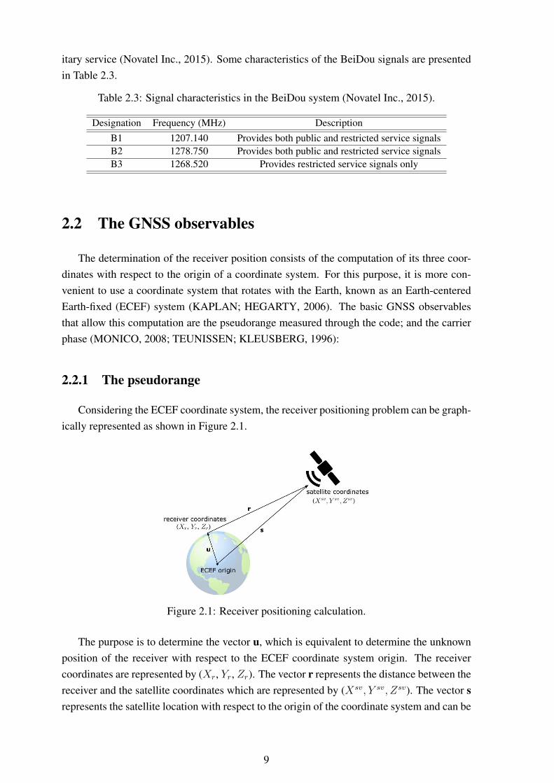
Designation Frequency (MHz) DescriptionB1 1207.140 Provides both public and restricted service signalsB2 1278.750 Provides both public and restricted service signalsB3 1268.520 Provides restricted service signals only

2.2 The GNSS observables

The determination of the receiver position consists of the computation of its three coor-dinates with respect to the origin of a coordinate system. For this purpose, it is more con-venient to use a coordinate system that rotates with the Earth, known as an Earth-centeredEarth-fixed (ECEF) system (KAPLAN; HEGARTY, 2006). The basic GNSS observablesthat allow this computation are the pseudorange measured through the code; and the carrierphase (MONICO, 2008; TEUNISSEN; KLEUSBERG, 1996):

2.2.1 The pseudorange

Considering the ECEF coordinate system, the receiver positioning problem can be graph-ically represented as shown in Figure 2.1.

Figure 2.1: Receiver positioning calculation.

The purpose is to determine the vector u, which is equivalent to determine the unknownposition of the receiver with respect to the ECEF coordinate system origin. The receivercoordinates are represented by (Xr, Yr, Zr). The vector r represents the distance between thereceiver and the satellite coordinates which are represented by (Xsv, Y sv, Zsv). The vector srepresents the satellite location with respect to the origin of the coordinate system and can be

9

calculated using the ephemeris data transmitted to the user (KAPLAN; HEGARTY, 2006).The subscript r and the superscript sv refer to as the coordinates of the receiver and thesatellite, respectively.

The measurement of the range between the satellite and the receiver antenna is based onthe code generated in the satellite and a replica generated in the receiver. These codes arerepresented by Gs(t) and Gr(t), respectively. By measuring the delay between a particulartransition in the code Gs(t) and the replica code Gr(t), the propagation time of the signal inthe path from the satellite to the receiver is obtained. The receiver measures this delay byusing the code cross-correlation. Figure 2.2 illustrates this principle (MONICO, 2008).

Satellite-generated

code

Receiver-generated

replica code

�t

Transmisson time

Arrival time

Propagation time

Figure 2.2: Use of replica code to determine the satellite code travelling time (MONICO,2008; KAPLAN; HEGARTY, 2006) (adapted).

The replica generated in the receiver is shifted until a high correlation between the signaltransmitted by the satellite and the replica generated at the receiver is reached. If the satelliteclock and the receiver clocks were perfectly synchronized, the correlation process wouldyield true propagation time. By multiplying the propagation time ∆t by the speed of light, c,the true (i.e. geometric) satellite-to-user range would be obtained. However, this is an idealscenario that considers the clocks synchronism. In general, the satellite and receiver clocksare not synchronized (KAPLAN; HEGARTY, 2006).

The receiver clock generally presents a bias with respect to the system time. Furthermore,although the time and frequency generation of the satellite is based in high accuracy atomicclocks (cesium and rubidium), the satellite clock also presents an offset with respect to thesystem time as well (KAPLAN; HEGARTY, 2006). Thus, due to the clock errors, the rangecalculated by using the correlation process is denoted as the pseudorange P (KAPLAN;HEGARTY, 2006).

The GNSS satellites have high precision atomic clocks operating in the satellite timesystem (tsv), to which all generated and transmitted signals are referenced. The receivers,in general, have lower quality oscillators that operate in the receiver time system (tr), towhich the received signals are referenced. For the GPS, these time systems, tsv and tr, can

10

be related to the GPS time system (tGPS) according to Equation (2.3) (MONICO, 2008).

tGPSsv = tsv − dtsv

tGPSr = tr − dtr,(2.3)

where, dtsv is the satellite clock error with respect to the GPS time at the instant tsv and dtris the receiver clock error with respect to the GPS time at the instant tr. The subscripts andsuperscripts refer the parameters related to the receiver and satellite, respectively (MONICO,2008).

The pseudorange (P svr ) is obtained by multiplying the velocity of light by the difference

between the time tr registered at the receiver in the instant of signal reception and the time tsv,registered at the satellite in the instant of signal transmission. Using the correlation processto obtain the propagation time, one can obtain the following expression for the pseudorange(MONICO, 2008; TEUNISSEN; KLEUSBERG, 1996):

P svr = c(tr−tsv) = c(tGPSr−tGPSsv)+c(dtr−dtsv)+εP = cτ svr +c(dtr−dtsv)+εP , (2.4)

where τ svr is the propagation time of the signal, counted from its generation at the satel-lite until the correlation at the receiver, c is the velocity of light at vacuum, and εP is thepseudorange measurement error (MONICO, 2008).

The propagation time τ svr multiplied by the velocity of light on vacuum does not resultin the geometric distance ρsvr between the antenna of the satellite and the receiver due toother sources of errors, such as the propagation effects of the atmosphere (e.g troposphericand ionospheric delays) and multipath. Thus, a more complete form for Equation (2.4) is(MONICO, 2008):

P svr = ρsvr + c(dtr − dtsv) + T svr + Isvr + dmsv

r + εP , (2.5)

where

ρsvr is the geometric distance from the satellite to the receiver;

T svr is the tropospheric delay (in meters);

Isvr is the ionospheric delay (in meters);

dmsvr is the multipath effect.

The coordinates of the receiver and the satellite are implicit in the term ρsvr as presentedin Equation (2.6).

ρsvr =

√(Xsv −Xr)

2 + (Y sv − Yr)2 + (Zsv − Zr)2. (2.6)

Applying (2.6) in (2.5), the pseudorange expression with the receiver and satellites coor-

11

dinates presented explicitly is given by:

P svr =

√(Xsv −Xr)

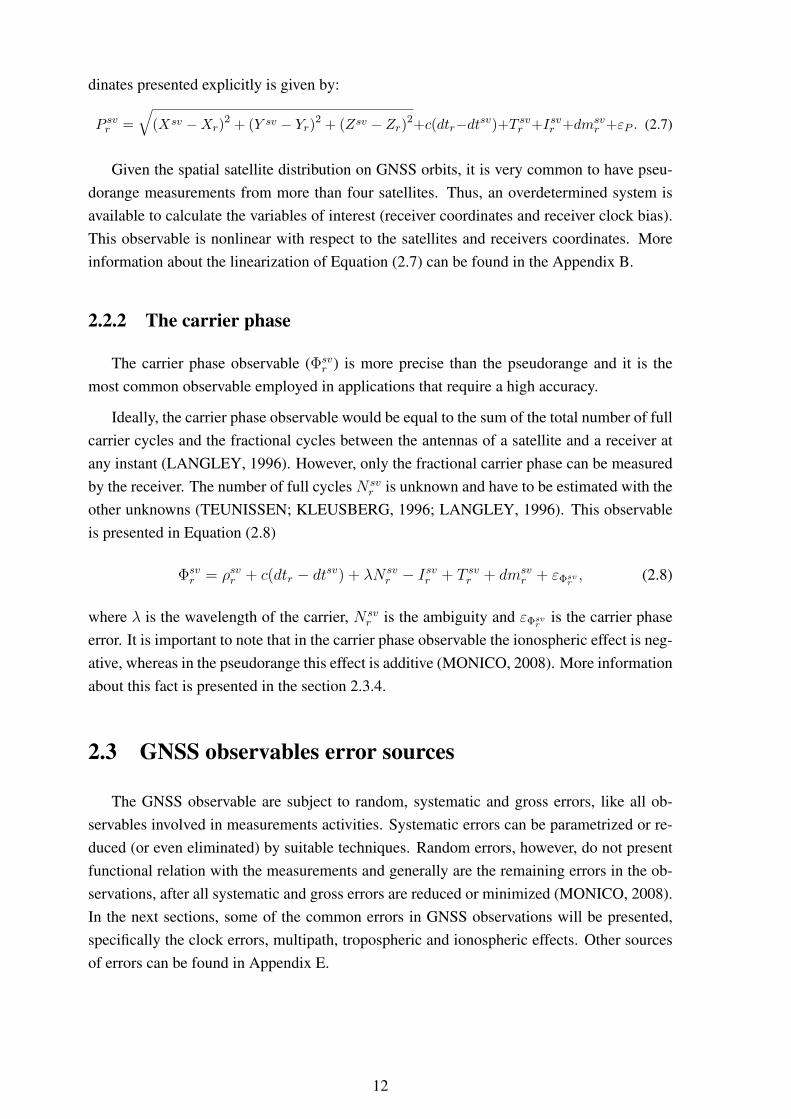
2 + (Y sv − Yr)2 + (Zsv − Zr)2+c(dtr−dtsv)+T svr +Isvr +dmsvr +εP . (2.7)

Given the spatial satellite distribution on GNSS orbits, it is very common to have pseu-dorange measurements from more than four satellites. Thus, an overdetermined system isavailable to calculate the variables of interest (receiver coordinates and receiver clock bias).This observable is nonlinear with respect to the satellites and receivers coordinates. Moreinformation about the linearization of Equation (2.7) can be found in the Appendix B.

2.2.2 The carrier phase

The carrier phase observable (Φsvr ) is more precise than the pseudorange and it is the

most common observable employed in applications that require a high accuracy.

Ideally, the carrier phase observable would be equal to the sum of the total number of fullcarrier cycles and the fractional cycles between the antennas of a satellite and a receiver atany instant (LANGLEY, 1996). However, only the fractional carrier phase can be measuredby the receiver. The number of full cycles N sv

r is unknown and have to be estimated with theother unknowns (TEUNISSEN; KLEUSBERG, 1996; LANGLEY, 1996). This observableis presented in Equation (2.8)

Φsvr = ρsvr + c(dtr − dtsv) + λN sv

r − Isvr + T svr + dmsvr + εΦsvr , (2.8)

where λ is the wavelength of the carrier, N svr is the ambiguity and εΦsvr is the carrier phase

error. It is important to note that in the carrier phase observable the ionospheric effect is neg-ative, whereas in the pseudorange this effect is additive (MONICO, 2008). More informationabout this fact is presented in the section 2.3.4.

2.3 GNSS observables error sources

The GNSS observable are subject to random, systematic and gross errors, like all ob-servables involved in measurements activities. Systematic errors can be parametrized or re-duced (or even eliminated) by suitable techniques. Random errors, however, do not presentfunctional relation with the measurements and generally are the remaining errors in the ob-servations, after all systematic and gross errors are reduced or minimized (MONICO, 2008).In the next sections, some of the common errors in GNSS observations will be presented,specifically the clock errors, multipath, tropospheric and ionospheric effects. Other sourcesof errors can be found in Appendix E.

12

2.3.1 Clock errors

2.3.1.1 Satellite clock errors

The satellite atomic clocks are monitored by the GNSS control segment and are veryprecise, however, they do not work perfectly synchronized with the GNSS reference time.From the data provided in the navigation message, it is possible to obtain the satellite clockcorrection dtsv for a satellite sv by the following second order polynomial (MONICO, 2008):

dtsv(t) = a0 + a1(tsv − toc) + a2(tsv − toc)2 + ∆tR, (2.9)

where

δsv is the satellite clock error on the instant t of the GNSS time scale;

tsv is the satellite reference epoch;

toc is the reference time of clock data;

a0 is the satellite clock offset coefficient, in seconds;

a1 in the satellite clock drift coefficient;

a2 is the satellite clock frequency drift coefficient;

∆tR = −2∗X ∗X/c2 is the correction for the relativistic effect on the satellite clock (X ,X and c are the position of the satellite, its velocity and the velocity of light, respectively).

2.3.1.2 Receiver clock errors

Differently from satellite clock errors, the receiver clock corrections in point positioningapplications need to be performed by the user. A brief description about point positioning ispresented in Appendix F. This procedure is done by the estimation of an additional parameterthat refers to the receiver clock synchronization error for every observation epoch. Using thisprocedure allows for the employment of small and inexpensive oscillators in the receivers,such as quartz crystal oscillators (WEINBACH; SCHöN, 2011; MONICO, 2008).

However, this type of clock estimation presents some associated drawbacks, such as theneed to observe at least four-satellites at the same time to determine the receiver position(three coordinates and one receiver clock off-set). Another point that has to be taken intoaccount is the degradation of the vertical position accuracy. This effect occurs due to theasymmetry on the observations, since only satellites in the hemisphere above the horizon areobserved. This fact leads to a mathematical correlation between receiver clocks, troposphereparameters and station height estimates (WEINBACH; SCHöN, 2011; M.ROTHACHER;G.BEUTLER, 1998).

In the relative positioning, the clock errors are almost eliminated, being not necessary touse highly stable clocks for the majority of applications. However, the simultaneity of the

13

observations has to be carefully taken into account. For high accuracy results, the receiverclock error in the relative positioning for each receiver involved in this technique has to beknown to 1 microsecond (1µs) with respect to the time system and the differences betweenthem cannot exceed 1 ms (MONICO, 2008).

2.3.2 Multipath

Considered one of the most significant sources of errors in satellite-based navigation sys-tems, the multipath may introduce errors in positioning calculations that could jeopardizehigh-precision applications (CLOSAS; FERNÁNDEZ-PRADES; FERNÁNDEZ-RUBIO,2009). Multipath is the phenomena in which the signal reaches the receiver by multiplepaths due to reflection and diffraction (BRAASCH, 1996). In other words, the receivers willget the signal which reaches directly the antenna and also signals reflected in the surfacesnearby. An illustration of the multipath is presented in Figure 2.3.

water

direct signal

reflected signal

Figure 2.3: Multipath illustration.

The signal received can present distortions on the carrier-phase and on modulation of thecarrier, and since the geometrical features in each place changes in an arbitrary way, thereis no model available to mitigate multipath. However, some techniques can be applied inorder to reduce this effect, including the use of antennas designed to supress low-elevation-angle signals, such as the choke ring and pinwheel, and its well-placement in suitable sites(ARBESSER-RASTBURG; ROGERS, 2013; BISHOP; KLOBUCHAR; DOHERTY, 1985;MONICO, 2008).

2.3.3 Tropospheric effect

The troposphere is the layer of atmosphere that starts from the Earth surface and extendsuntil 50 km, approximately. It behaves like a non-dispersive medium for frequencies below30 GHz, i.e. the refraction of the transmitted signal does not depend on the signal frequency.It depends only on the thermodynamic properties of the air (MONICO, 2008). The specifictropospheric effects on the GNSS L-band signals include tropospheric attenuation, tropo-

14

spheric scintillation and tropospheric delay (SPILKER, 1996). This section presents a quickoverview of the tropospheric effect on GNSS signals. Additional information can be foundin the Appendix C.

2.3.3.1 Tropospheric attenuation

The tropospheric attenuation varies for each frequency and corresponds to the reductionof power of the electromagnetic wave due to the elements that compose the atmosphere(MONICO, 2008; SPILKER, 1996). In the 1-2 GHz frequency band, it is dominated byoxygen attenuation. For a satellite at zenith, the attenuation is about 0.035 dB. The effects ofwater vapor, rain and nitrogen attenuation is negligible at GNSS frequency bands (SPILKER,1996). For GNSS signals it is not recommended to use observations obtained at elevationangles lower than 5◦, since the ray path to the satellite penetrates the lower troposphere ina more nearly horizontal direction leading to a higher signal attenuation (SPILKER, 1996).In practice, it is common to use elevation angles higher than 15◦, commonly referred to aselevation mask (MONICO, 2008). More information about the tropospheric attenuation as afunction of the elevation angle can be found in Appendix C.

2.3.3.2 Tropospheric delay

The delay on the GNSS signals when traveling through the troposphere is caused mainlyby the neutral hydrostatic atmosphere (composed of dry gases), corresponding to 90% ofthe total effect. The remaining 10% depends on the water vapor 3D distribution (non-hydrostatic component), which is hard to estimate, due to its high temporal and spatial vari-ations (HADAS et al., 2013; SAPUCCI, 2001).

The hydrostatic component of the tropospheric delay corresponds to 2.3 m on zenithand varies with temperature and local atmospheric pressure. Since its variation is small (inthe order of 1% over several hours), this component is predicted with reasonable precision.The wet effect, caused by the atmospheric water vapor influence, is less than the hydrostaticcomponent, varying from 1 to 35 cm in zenith, corresponding to 10% of the total troposphericdelay (SEEBER, 2003; MONICO, 2008). However, although its low effect, its variationis considerable, reaching 20% in a few hours, making impossible its prediction with goodprecision, even when there is availability of superficial humidity measurements (MONICO,2008).

In general, the models to estimate tropospheric delay in the path between the receiverantenna r and the satellite sv are presented as

T sr = 10−6

∫NTds. (2.10)

The troposphere refractivity is given by NT = (n − 1) × 106, where n is the refractive

15

index. The hydrostatic and wet components of the tropospheric delay can be written as theproduct between the zenith delay and a mapping function which relates the vertical delaywith the slant delay. Therefore, the tropospheric delay can be expressed as

T sr = TZH ×mh(ε) + TZW ×mw(ε), (2.11)

where TZH and TZW corresponds, respectively, to the hydrostatic and wet components ofthe tropospheric delay in the zenith direction. The mh(ε) and mw(ε) values are the cor-responding mapping functions used to convert the zenith delay to slant delay (MONICO,2008).

In order to determine the tropospheric delay T sr it is necessary to obtain the refractiv-ity NT . By the knowledge of NT and its hydrostatic (NH) and wet (NW ) components it ispossible to determine the terms TZH and TZH , and consequently, T sr by using the mappingfunctions. The determination of the refractivity along the signal path is almost impossible(SAPUCCI, 2001). This is the reason why several models have been developed to describethe behavior of this variable. More information about the tropospheric models and the map-ping functions can be found in Appendix C.

2.3.4 Ionospheric effect

The ionosphere is the Earth atmosphere region where ionizing radiation causes the ex-istence of electrons in an amount that affects radio waves propagation (LANGLEY, 1992).The energy radiated from the sun at ultraviolet and X-ray wavelengths is the primary forceof ionosphere formation. This force ionizes gaseous atoms and molecules in the atmosphere,producing positively charged ions and negatively charged free electrons (WEBSTER, 1993).In order to describe the amount of charged particles in the ionosphere, the term electrondensity (Ne) is used (HABARULEMA et al., 2009).

The ionosphere is composed of four regions, D, E, F1 and F2, named in order of increas-ing height. Each region presents particular electron density features (KLOBUCHAR, 1996).Table 2.4 presents some characteristics of the ionospheric regions, such as the height of eachlayer, and information about its impact on GNSS signals.

As described in Section 2.3.3.2, the tropospheric range error at zenith is generally be-tween two to three meters. The ionospheric range error, on the other hand, can vary fromonly a few meters to many tens of meters at the zenith (KLOBUCHAR, 1996). When com-pared to the tropospheric effect, the variability of the ionospheric effect is much larger andit is more difficult to model. Furthermore, ionosphere can have significant effects on GNSS,such as: group delay of the signal modulation, or absolute range error; carrier phase advance,relative range error; Doppler shift, or range-rate errors; Faraday rotation of linearly polar-ized signals; refraction or bending of the radio wave; distortion of pulse waveforms; signalamplitude fading or amplitude scintillation; and phase scintillations. (KLOBUCHAR, 1996;

16

Table 2.4: Characteristics of the different regions of the ionosphere (KLOBUCHAR, 1996).

Region Approx. Height (km) RemarkD 50 to 90 Causes absorption of radio signals at frequencies up to

low VHF band. It has no measurable effect on GNSSE 90 to 140 Normal E region, caused by solar soft

x-rays. It has minimal effect on GNSS.Intense E region, caused by solar particle precipitation

in aurora region, might cause minimal scintillation.Sporadic E (still of unknown origin). It is very thin.

The effect on GNSS frequencies is neglected.F1 140 to 210 It has a highly predictable density from known

solar emissions. Its electron density nicely merges intothe bottomside of the F2 region.

F2 210 to 1000 It is the most dense and it has the highest variability.The peak of electron density generally varies from 250

to 400 km, but it can differs at extreme conditions.This region, with to some extension the F1, cause most of theproblems for radio-wave propagation at GNSS frequencies.

HOQUE; JAKOWSKI, 2012).

The interaction between the GNSS radio signals and the ionospheric plasma is one of themajor reasons for the limited accuracy and vulnerability in GNSS positioning solutions ortime estimation (HOQUE; JAKOWSKI, 2012). Even at this relatively high frequency, theEarth ionosphere can retard radio waves from their velocity in free space by more than 300nson a worst case basis, corresponding to range errors of 100m (JAKOWSKI et al., 2011).

An electromagnetic wave is not affected when traveling through a static electric or mag-netic field in a linear medium such as vacuum. However, traveling through the ionosphere,which is a dispersive medium (i.e. the velocity of the electromagnetic wave is a function of itsfrequency), different aspects cause variation on the polarization, propagation speed and sig-nal power (BORRE; STRANG, 2012; HOQUE; JAKOWSKI, 2015; HOQUE; JAKOWSKI,2012). In the context of L band signals of GNSS, the ionospheric refraction, proportional tothe TEC value, introduces most of the delay and may cause link-related range errors in thepositioning system of up to 100 m (HOQUE; JAKOWSKI, 2015). Three different dynamicprocesses contribute to strong temporal and spatial variation of TEC in the equatorial andlow-latitude sectors: the equatorial ionization anomaly, post-sunset plasma enhancement andevening plasma bubbles, leading to an even worst scenario in these regions (TAKAHASHIet al., 2014).

The propagation of an electromagnetic wave passing through the ionosphere is quantita-tively described by the refractive index of the ionosphere (HOQUE; JAKOWSKI, 2012). Forradio waves with frequency f greater than 100 MHz, the phase refractive index n and thegroup refractive index ngr derived from the Appleton-Hartree equation are given by Equa-

17

tions (2.12) and (2.13).

n = 1−f 2p

2f 2±f 2p fgcosΘ

2f 3−

f 2p

4f 4

[f 2p

2+ f 2

g (1 + cos2Θ)

], (2.12)

ngr = 1 +f 2p

2f 2∓f 2p fgcosΘ

f 3+

3f 2p

4f 4

[f 2p

2+ f 2

g (1 + cos2Θ)

], (2.13)

in which Θ is the angle between the wave propagation direction and the geomagnetic fieldvector B and fp and fg are the plasma frequency and gyro frequency given by

fp2 = Nee

2/(4π2ε0m),

fg = eB/(2πm),(2.14)

where ε0 is the free space permittivity, B is the geomagnetic induction, and e, Ne, m are theelectron charge, density and mass, respectively (HOQUE; JAKOWSKI, 2012). The expres-sion presented in Equation (2.13) can be obtained by the relationship ngr = n + f(dn/df)

(HOQUE; JAKOWSKI, 2012; HARTMANN; LEITINGER, 1984; APPLETON, 1932). Thepositive and negative signals in the equations ± and ∓ are related with the polarization ofthe wave, which means that the (+) sign represents the refractive index for left-hand cir-cularly polarized wave, whereas the (-) represents the right-hand circularly polarized wave.(HOQUE; JAKOWSKI, 2012; HARTMANN; LEITINGER, 1984). The GPS signals aretransmitted in right-hand circular polarization (DoD, 2012).

By analyzing Equations (2.12) and (2.13) one can note that the phase refractive indexis less than the unity resulting in a phase velocity that is greater than the speed of light inthe vacuum (i.e., phase advance). Thus, when GNSS signals propagate through the iono-sphere, the carrier-phase experiences an advance and the code experiences a group delay.The carrier-phase pseudoranges are measured too short and the code pseudoranges are mea-sured too long compared to the geometric range between a satellite and a receiver (HOQUE;JAKOWSKI, 2012).

2.3.4.1 Total Electron Content

By using Equations (2.12) and (2.13) and assuming a right-hand circularly polarizedsignal, the ionospheric group delay dIgr and the carrier phase advance dI , written in units oflength, in the path s from the satellite to the receiver are given by (HOQUE; JAKOWSKI,2012)

dIgr = d(1)Igr + d

(2)Igr + d

(3)Igr =

∫s

(ngr − 1)ds =p

f 2+

q

f 3+

u

f 4, (2.15)

dI = d(1)I + d

(2)2 + d

(3)I =

∫s

(1− n)ds =p

f 2+

q

2f 3+

u

3f 4, (2.16)

18

in which the terms d(1)Igr / d(1)

I , d(2)Igr / d(2)

2 , and d(3)Igr / d(3)

I are the first, second and third orderionospheric group delays / phase advances, respectively. The coefficients p, q and u aregiven by

p = 40.3

∫s

Neds, (2.17)

q = 2.2566× 1012

∫s

NeBcosΘds, (2.18)

u = 2437

∫Ne

2ds+ 4.74× 1022

∫s

NeB(1 + cos2Θ)ds. (2.19)

The result of the integration of Ne along the signal path∫sNeds is known as the slant

Total Electron Content (slant TEC). This parameter is defined as the amount of electrons in acolumn of cross sectional area of 1 m2 along the path of the signal through the ionosphere andis expressed in TECU (1 TECU is equivalent to 1 x 1016 electrons/m2) (HABARULEMAet al., 2009). Considering the GPS, 1 TECU corresponds to a ionospheric delay of 0.163 mon L1 and 0.267 m on L2 signals (DYRUD et al., 2008).

When the GNSS signals are transmitted in two different signals, the non-dispersive ef-fects, such as, tropospheric delay, satellite and receiver clocks biases affects equally bothfrequencies. The ionospheric effect, however, affects differently each frequency. Therefore,by differencing the code/carrier-phase pseudoranges measurements of the two frequenciesit is possible to estimate the TEC along the path between the satellite and the receiver, asshown in Equations 2.20 and 2.21 (HOQUE; JAKOWSKI, 2012).

TEC =f 2

1 f22

40.3(f 21 − f 2

2 )[(P2− P1) + noiseP1−P2], (2.20)

TEC =f 2

1 f22

40.3(f 21 − f 2

2 )[(Φ1− Φ2) +Bambiguity + noiseΦ1−Φ2], (2.21)

where P1 and P2 are pseudoranges obtained using the L1 and L2 signals, respectively; Φ1

and Φ2 are the carrier-phase measurements, the noiseP1−P2 and noiseΦ1−Φ2 are noises (e.gthermal noises, etc) in the code and carrier-phase combinations, Bambiguity is the carrier-phase constant ambiguity which is equal to λ2N2 − λ1N1, with λ1 and λ2 correspondingto the wavelengths and N1 and N2 corresponding to the integer ambiguities on frequenciesf1 and f2. The terms corresponding to other effects, such as, multipath and inter-frequencysatellite and receiver biases are not presented in Equations 2.20 and 2.21 for simplicity rea-sons (HOQUE; JAKOWSKI, 2012).

The ionospheric effect is still one of the major error sources of GNSS positioning forsingle-frequency users (LIU et al., 2016). The first order term presented in Equations (2.15)and (2.16) includes about 99% of the total ionospheric effect. Therefore, if the frequencyand the related slant TEC are known, the first order propagation effect can easily be com-puted and corrected. To compensate this effect, several approaches can be adopted. The

19

ionosphere free combination (IF) takes advantages of the dispersive character of the iono-sphere to eliminate this first-order effect (ELMAS et al., 2011). This approach is based onmulti-frequency satellite-receiver communication. Single-frequency receivers, however, cannot take advantage of IF. In this case, observations need to be corrected by the use of externalmodels in order to eliminate the first order ionospheric error contribution (PAPARINI et al.,2016). Information about some models available are presented in the next section.

2.3.4.2 Ionospheric models

The ionospheric models available are classified into empirical and physics based. Theempirical models are developed based on long-term measurements and statistical analy-sis, whereas the physics-based models rely on a complete understanding of the under-lying physics and commonly starts from an empirical model of the neutral atmosphere(MITCHELL, 2013). Some common ionospheric models are presented below:

a) Klobuchar - The Klobuchar model received the name of his proposer John A.Klobuchar and was developed at the Air Force Geophysics Laboratory, U.S. This is avery known simple mathematical model that represents the ionosphere using a heuris-tic approach to finding a fit to some known observations. The purpose in designingthis model is to provide a simple and fast ionospheric time-delay correction algorithmfor the single-frequency users of GPS. The idea is to use a few coefficients, leadingto a lesser computational effort to compensate for 50% of the ionospheric time-delay(KLOBUCHAR, 1987; MITCHELL, 2013).

The algorithm, incorporated in the GPS system for single-frequency users, consists of acosine representation of the diurnal curve, allowed to vary in amplitude and in period,with user latitude. Its shape is determined by using eight coefficients, transmittedas part of the satellite message. Figure 2.4 presents an example in which a positivehalf cosine-shaped curve has been made to fit a typical monthly average TEC diurnalvariation from an station in Jamaica using the referred model (KLOBUCHAR, 1987).

b) NeQuick - The NeQuick model is a quick-run model for transionospheric applicationsdeveloped at the Abdus Salam ICTP Aeronomy and Radiopropagation Laboratory,Italy, with collaboration of the University of Graz Institute for Geophysics, Astro-physics and Meteorology, Austria. This model provides electron concentration at thegiven location in space and time (Ne) and its basic inputs are position, time, and solarflux (or sunspot number). The NeQuick package allows to compute the electron den-sity along any-ray path and by numerical integration provides the TEC to the user. Itsoriginal version has been used by the European Navigation Overlay Service (EGNOS)of the European Space Agency (ESA) for system assessment analysis.

One very important use of the NeQuick model is its adoption as the model for iono-spheric corrections for single frequency users on the GALILEO system. To be used in

20

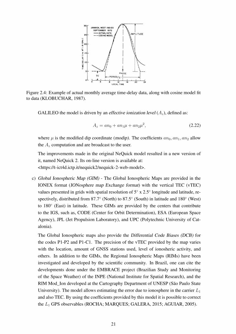
Figure 2.4: Example of actual monthly average time-delay data, along with cosine model fitto data (KLOBUCHAR, 1987).

GALILEO the model is driven by an effective ionization level (Az), defined as:

Az = an0 + an1µ+ an2µ2, (2.22)

where µ is the modified dip coordinate (modip). The coefficients an0, an1, an2 allowthe Az computation and are broadcast to the user.

The improvements made in the original NeQuick model resulted in a new version ofit, named NeQuick 2. Its on-line version is available at:<https://t-ict4d.ictp.it/nequick2/nequick-2-web-model>.

c) Global Ionospheric Map (GIM) - The Global Ionospheric Maps are provided in theIONEX format (IONosphere map Exchange format) with the vertical TEC (vTEC)values presented in grids with spatial resolution of 5◦ x 2.5◦ longitude and latitude, re-spectively, distributed from 87.7◦ (North) to 87.5◦ (South) in latitude and 180◦ (West)to 180◦ (East) in latitude. These GIMs are provided by the centers that contributeto the IGS, such as, CODE (Center for Orbit Determination), ESA (European SpaceAgency), JPL (Jet Propulsion Laboratory), and UPC (Polytechnic University of Cat-alonia).

The Global Ionospheric maps also provide the Differential Code Biases (DCB) forthe codes P1-P2 and P1-C1. The precision of the vTEC provided by the map varieswith the location, amount of GNSS stations used, level of ionosheric activity, andothers. In addition to the GIMs, the Regional Ionospheric Maps (RIMs) have beeninvestigated and developed by the scientific community. In Brazil, one can cite thedevelopments done under the EMBRACE project (Brazilian Study and Monitoringof the Space Weather) of the INPE (National Institute for Spatial Research), and theRIM Mod_Ion developed at the Cartography Department of UNESP (São Paulo StateUniversity). The model allows estimating the error due to ionosphere in the carrier L1

and also TEC. By using the coefficients provided by this model it is possible to correctthe L1 GPS observables (ROCHA; MARQUES; GALERA, 2015; AGUIAR, 2005).

21

In addition to the models presented herein, some modeling activities based on ArtificialNeural Networks (NNs) have been carried out. The use of NNs has provided good results inthe modeling of the regional TEC, being capable of recovering TEC values with good per-formance (HABARULEMA et al., 2009; LEANDRO; SANTOS, 2007). This fact is relatedto the abilities of a NN to learn, generalize and adapt to different patterns of input/output setswith nonlinear behavior (HAYKIN, 1999).

In this framework, this manuscript presents a NN regional model to estimate TEC behav-ior based on GNSS measurements in three different regions in Brazil (Northeast, Central-West and South regions). The next section presents general information and concepts aboutthe Neural Networks, emphasizing the Multilayer Perceptron (MLP) structures since thisclass of NN formed the basis for the vTEC estimations performed in this work.

2.4 Artificial Neural Networks

An Artificial Neural Network (ANN) is a massively parallel distributed processor madeup of simple processing units that has a natural propensity for storing experiential knowledgeand making it available for use (HAYKIN, 2009). This network is inspired in biologicalneuronal systems (HAYKIN, 2009) and has been employed in studies in different fields,including applications on ionospheric modelling (HABARULEMA et al., 2009; LEANDRO;SANTOS, 2007; WILLISCROFT; POOLE, 1996).

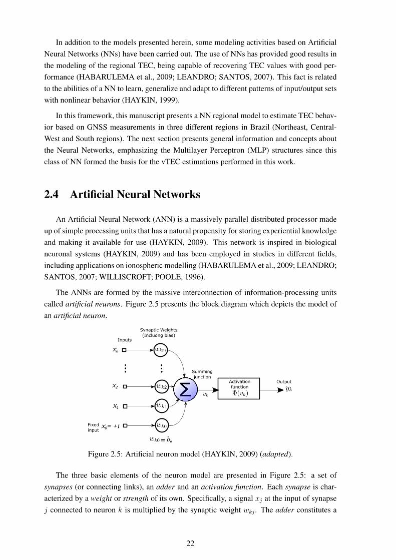
The ANNs are formed by the massive interconnection of information-processing unitscalled artificial neurons. Figure 2.5 presents the block diagram which depicts the model ofan artificial neuron.

Inputs

Activation

function

Synaptic Weights

(Includng bias)

Summing

junctionOutput

Fixed

inputx0= +1

x1

x2

xm

=

Figure 2.5: Artificial neuron model (HAYKIN, 2009) (adapted).

The three basic elements of the neuron model are presented in Figure 2.5: a set ofsynapses (or connecting links), an adder and an activation function. Each synapse is char-acterized by a weight or strength of its own. Specifically, a signal xj at the input of synapsej connected to neuron k is multiplied by the synaptic weight wkj . The adder constitutes a

22

linear combiner in which the input signals weighted by the respective synaptic strengths aresummed. The role of the activation function is also to limit the amplitude of a neuron. Itlimits the permissible amplitude range of the output signal to some finite value. The modelpresented in Figure 2.5 also includes an externally applied bias, bk, which has the effect ofincreasing or lowering the net input of the activation function, depending on whether it ispositive or negative, respectively (HAYKIN, 2009).

2.4.1 Rosenblatt perceptron

The Rosenblatt perceptron is built around a single neuron and is the simplest form of aneural network. It consists of a neuron as the one presented in Figure 2.5 with adjustablefree parameters (synaptic weight and bias). For a given set of inputs, the neuron producesan output equal to +1 if the activation function input is positive, and -1 if it is negative. Thealgorithm used to adjust the free parameters of this type of NN appeared for the first time ina learning procedure developed by Rosenblatt (1958, 1962) for his perceptron brain model(HAYKIN, 2009).

The goal of the single-neuron perceptron is to classify the input set into one of two classesC1 or C2. Depending on the output of the network, +1 or -1, the point represented by inputsx1, x2, ..., xm will be assigned to class C1 or C2, respectively.

To develop insight into the behavior of a pattern classifier, it is customary to plot a mapof the decision regions in the m-dimensional signal space spanned by the m input variablesx1, xm, ..., xm. In the single-neuron perceptron, there are two decision regions separated bya hyperplane, which is defined by

m∑i=1

wixi + b = 0. (2.23)

For the case of two input variables x1 and x2, the hyperplane is given by w1x1 +w2x2 +

b = 0. In this case, the decision boundary (hyperplane) takes the form of a straight line.A point (x1, x2) which lies below the line can be classified as C2 and a point (x1, x2) abovethe line can be classified as C1. Figure 2.6 illustrates this decision boundary. It is possibleto see that the bias b plays the role of shifting the decision boundary away from the origin(HAYKIN, 2009).

2.4.2 Multilayer Perceptron

The Rosenblatt perceptron, which is basically a single-layer neural network, is limitedto the classification of linearly separable patterns (HAYKIN, 2009). To overcome this limi-tation a neural network structure that can be used is the Multilayer Perceptron (MLP). Thisstructure contains one or more layers that are hidden from both the input and output and

23

0

Decision boundary

Figure 2.6: Hyperplane as a decision boundary for a two-dimensional, two-class pattern-classification problem (HAYKIN, 2009) (adapted).

presents a high degree of connectivity between the neurons. In addition, the neuron modelused in the network includes a nonlinear activation function that is differentiable (HAYKIN,2009). The sigmoid functions are the most common type of activation functions applied inneural networks. Its name is derived from the shape of its graph which is presented in a "S-shape" (HAYKIN, 2009). One example of sigmoid function is the logistic sigmoid functiondescribed by

Φ(v) =1

1 + exp(−av), (2.24)

where a is the slope parameter of the function.

In some cases, it is desirable that the activation function assumes positive and negativevalues, from -1 to +1. This kind of activation function may yield practical benefits over thelogistic function described in Equation (2.24). In this case, the hyperbolic tangent functiondescribed in Equation (2.25) can be used.

Φ(v) =exp(v)− exp(−v)

exp(v) + exp(−v). (2.25)

2.4.2.1 Function approximation

The MLP structure can be employed in the function approximation task (HAYKIN,2009). Consider a nonlinear input-output mapping described by

d = f(x) (2.26)

where x and d are the input and output vectors, respectively. The vector-valued function f

is assumed to be unknown. In order to compensate the lack of knowledge about f , the set of

24

training samples T composed of labeled examples is given

T = {(xi,di)Ni=1}. (2.27)

The requirement is to develop a neural network that approximates the unknown function f ina certain way that the following Euclidean distance over all inputs, such that

‖F(x)− f(x)‖ < ε, for all x, (2.28)

where ε is a small positive number and F describes the input-output mapping actually re-alized by the NN. Considering that the size N of the training set T is large enough andthe network has the suitable number of free parameters, then the approximation error canbe made small enough for the proposed task. This sort of approximation can be seen as acandidate for the supervised learning procedure, which requires the availability of a targetresponse for performing a specific input-output mapping by minimizing a cost function ofinterest, with xi being the input vector, di being the desired response, in which the index irepresents the i-th input-output pair of the training set. In this function approximation sce-nario, a MLP containing only one hidden layer is capable to approximate any continuousfunction (CYBENKO, 1989; MACHADO, 2012).

In order to perform the supervised learning of the MLPs, the Back-Propagation algorithmis frequently used. During the training procedure, the parameters (degrees of freedom orsynaptic weights and bias) are adjusted aiming to minimize a cost function which allowsassessing the quality of the solution (MACHADO, 2012). This procedure is an iterativeprocess in which the updates of the synaptic weight connecting neuron k to neuron j arecalculated according to the following equation

wkj(n+ 1) = wkj(n) + ∆wkj(n) (2.29)

where w is the synaptic weight, n is the update step and ∆w is the correction applied tothe synaptic weight (MACHADO, 2012). The correction ∆wkj(n) is defined by (HAYKIN,2009)

∆wkj(n) = ηδj(n)yk(n), (2.30)

where η is the learning-rate, the term δj(n) is the local gradient and its value depends onwhether the neuron j is located in the output layer or in the hidden layer (HAYKIN, 2009):

1 If the neuron j is located in the output layer, δj(n) is equal to the product of thederivative Φj

′(vj(n)) and the error signal ej(n), which is defined by the differencebetween the NN output yj(n) and the desired output dj;

2 If the neuron j is located in a hidden layer, δj(n) is equal to the product of the asso-ciated derivative Φj

′(vj(n)) and the weighted sum of the δ values computed for theneurons in the next hidden or output layer that are connected to neuron j.

25

As presented previously, this work proposes the use of NN for TEC modelling in theBrazilian region. The detailed information about the investigated NN models is presented inthe next section.

26

Chapter 3

Results and analysis

This work presents different studies performed in order to investigate the use of ArtificialNeural Networks on vTEC estimation in the Brazilian region. These distinct studies considerdifferent input parameters for the network, distinct vTEC calibration techniques, differentperiods and, in some cases, different stations. The studies will be, henceforward, referred toas Case study 1, 2 and 3. In the first two case studies, the spatial performance of the ANN isassessed. The third case study presents an extended analysis of the ANN model, includingits capability to perform short-term forecasting and its comparison with the GIMs.

To perform the analysis, data from some stations of the Brazilian Network for Contin-uous Monitoring of the GNSS (RMBC) were used on TEC calibration and from the firstGLONASS network for research and development (GLONASS R&D network) installed inLatin America were used in this work.

3.1 Preliminaries

This preliminary section presents to the reader some common information for the threeCase studies shown in this work. This section includes information about the types of inputparameters, employed TEC calibration techniques and the adopted indexes to assess thenetwork performance.

3.1.1 NN model input parameters

TEC magnitude is influenced by solar activity, geographic location, Earth magnetic fieldand presents diurnal and seasonal variations (HOFMANN-WELLENHOF; LICTHENEG-GER; WASLE, 2008; MONICO, 2008). Therefore, the chosen input parameters for thecases under investigation presented in this work can include the latitude, longitude, solar ra-dio flux (F10.7), time of the day, day of year (doy), Dst-index and Kp-index. The set of inputparameters for each case study will be presented in its corresponding section.

27

Geographic location

Geographic location has a strong influence in the ionosphere electron density variation(BHUYAN; BORAH, 2007; MONICO, 2008). Although a gross generalization, equato-rial regions are characterized by high levels of electron density, mid-latitude regions areconsidered relatively free of ionospheric anomalies and polar regions of the Earth are veryunpredictable (WEBSTER, 1993).

Solar radio flux

The solar radio flux (F10.7) index is a determination of the strength of the solar radioemission in a 100 MHz-wide band centered on a 2800 MHz, corresponding to a 10.7 cmwavelength. It is one of the most common indexes used to interpret solar activity. Althoughit is commonly referred to as a flux, this index is a flux density (TAPPING, 2013). Severalfields can be benefited by the research and prediction of F10.7, such as the safety of spacecraft,the safety of space and air travel, and others (ZHAO; HAN, 2008).

Solar radio flux data used in this work were obtained from Laboratory for Atmosphericand Space Physics - University of Colorado Boulder (LASP) database, available on-line 1.

Seasonal variation

Season is another factor that influences electron density variation due to changes inthe zenith angle of the Sun and in the radiation flux intensity. During equinoxes, iono-spheric effects are greater, whereas during the solstices the ionosphere effects are smaller(HOFMANN-WELLENHOF; LICTHENEGGER; WASLE, 2008; MONICO, 2008).

Different periods are considered in this work, the first (from doy 154 to 163) is a ten-days period at the end of Brazilian autumn, and the second period (from doy 282 to 291) isa ten-days period on Brazilian spring. A third period, from doy 264 to 268, which includesthe September equinox of 2016 is investigated in the Case study 2.

Dst-index

The Disturbance Storm Time (Dst) index was designed to reveal the global magneticfield reductions during storms. This is one of the most widely used indexes to describe spacestorm activity. This index is given in nanotesla and it is provided on an hourly basis.

Dst data used in this work were obtained from the World Data Center (WDC) for Geo-magnetism archive available on-line 2.

1<http://lasp.colorado.edu/lisird/data/noaa_radio_flux/>2<http://wdc.kugi.kyoto-u.ac.jp/dstdir/index.html>

28

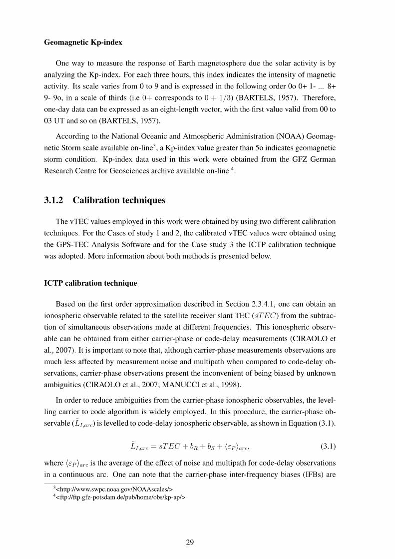
Geomagnetic Kp-index

One way to measure the response of Earth magnetosphere due the solar activity is byanalyzing the Kp-index. For each three hours, this index indicates the intensity of magneticactivity. Its scale varies from 0 to 9 and is expressed in the following order 0o 0+ 1- ... 8+9- 9o, in a scale of thirds (i.e 0+ corresponds to 0 + 1/3) (BARTELS, 1957). Therefore,one-day data can be expressed as an eight-length vector, with the first value valid from 00 to03 UT and so on (BARTELS, 1957).

According to the National Oceanic and Atmospheric Administration (NOAA) Geomag-netic Storm scale available on-line3, a Kp-index value greater than 5o indicates geomagneticstorm condition. Kp-index data used in this work were obtained from the GFZ GermanResearch Centre for Geosciences archive available on-line 4.

3.1.2 Calibration techniques

The vTEC values employed in this work were obtained by using two different calibrationtechniques. For the Cases of study 1 and 2, the calibrated vTEC values were obtained usingthe GPS-TEC Analysis Software and for the Case study 3 the ICTP calibration techniquewas adopted. More information about both methods is presented below.

ICTP calibration technique

Based on the first order approximation described in Section 2.3.4.1, one can obtain anionospheric observable related to the satellite receiver slant TEC (sTEC) from the subtrac-tion of simultaneous observations made at different frequencies. This ionospheric observ-able can be obtained from either carrier-phase or code-delay measurements (CIRAOLO etal., 2007). It is important to note that, although carrier-phase measurements observations aremuch less affected by measurement noise and multipath when compared to code-delay ob-servations, carrier-phase observations present the inconvenient of being biased by unknownambiguities (CIRAOLO et al., 2007; MANUCCI et al., 1998).

In order to reduce ambiguities from the carrier-phase ionospheric observables, the level-ling carrier to code algorithm is widely employed. In this procedure, the carrier-phase ob-servable (LI,arc) is levelled to code-delay ionospheric observable, as shown in Equation (3.1).

LI,arc = sTEC + bR + bS + 〈εP 〉arc, (3.1)

where 〈εP 〉arc is the average of the effect of noise and multipath for code-delay observationsin a continuous arc. One can note that the carrier-phase inter-frequency biases (IFBs) are

3<http://www.swpc.noaa.gov/NOAAscales/>4<ftp://ftp.gfz-potsdam.de/pub/home/obs/kp-ap/>

29

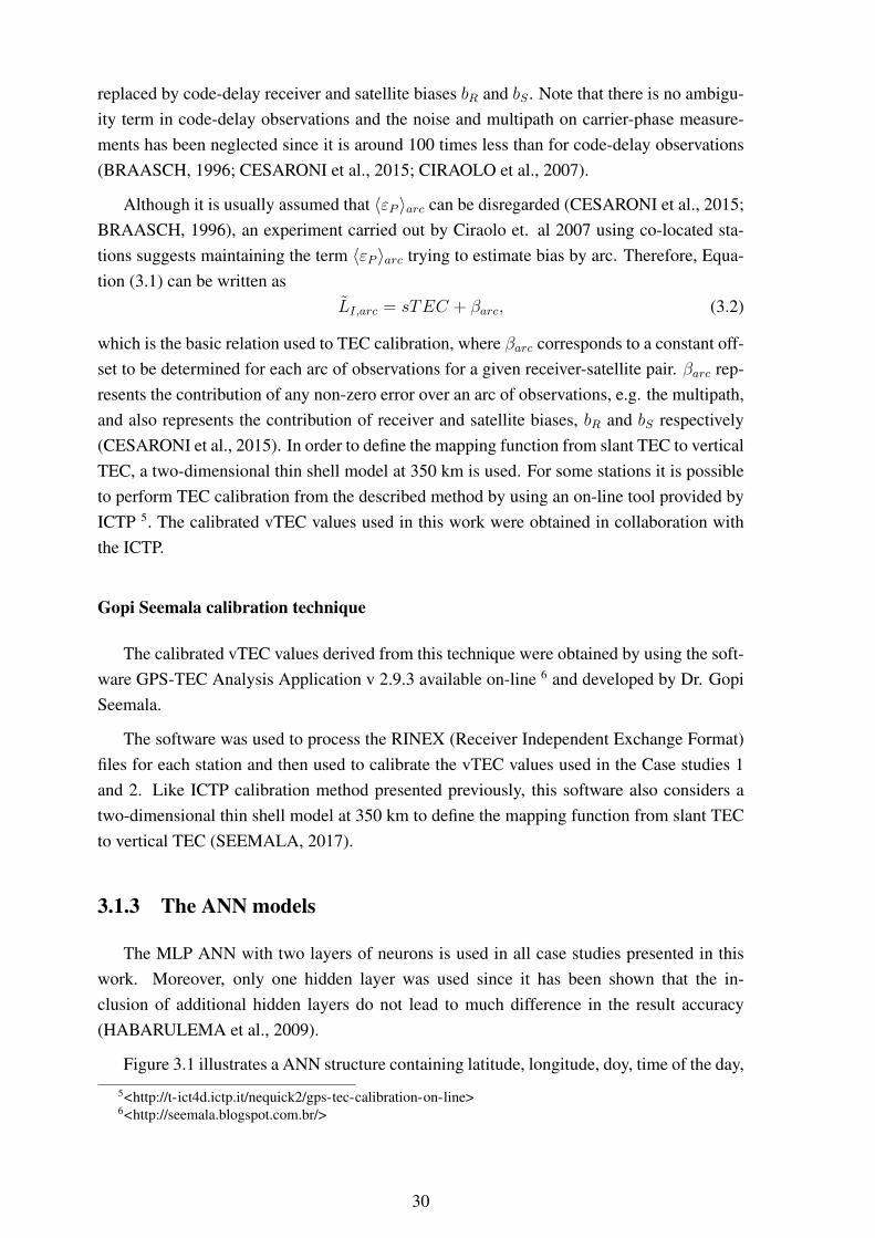
replaced by code-delay receiver and satellite biases bR and bS . Note that there is no ambigu-ity term in code-delay observations and the noise and multipath on carrier-phase measure-ments has been neglected since it is around 100 times less than for code-delay observations(BRAASCH, 1996; CESARONI et al., 2015; CIRAOLO et al., 2007).

Although it is usually assumed that 〈εP 〉arc can be disregarded (CESARONI et al., 2015;BRAASCH, 1996), an experiment carried out by Ciraolo et. al 2007 using co-located sta-tions suggests maintaining the term 〈εP 〉arc trying to estimate bias by arc. Therefore, Equa-tion (3.1) can be written as

LI,arc = sTEC + βarc, (3.2)

which is the basic relation used to TEC calibration, where βarc corresponds to a constant off-set to be determined for each arc of observations for a given receiver-satellite pair. βarc rep-resents the contribution of any non-zero error over an arc of observations, e.g. the multipath,and also represents the contribution of receiver and satellite biases, bR and bS respectively(CESARONI et al., 2015). In order to define the mapping function from slant TEC to verticalTEC, a two-dimensional thin shell model at 350 km is used. For some stations it is possibleto perform TEC calibration from the described method by using an on-line tool provided byICTP 5. The calibrated vTEC values used in this work were obtained in collaboration withthe ICTP.

Gopi Seemala calibration technique

The calibrated vTEC values derived from this technique were obtained by using the soft-ware GPS-TEC Analysis Application v 2.9.3 available on-line 6 and developed by Dr. GopiSeemala.

The software was used to process the RINEX (Receiver Independent Exchange Format)files for each station and then used to calibrate the vTEC values used in the Case studies 1and 2. Like ICTP calibration method presented previously, this software also considers atwo-dimensional thin shell model at 350 km to define the mapping function from slant TECto vertical TEC (SEEMALA, 2017).

3.1.3 The ANN models

The MLP ANN with two layers of neurons is used in all case studies presented in thiswork. Moreover, only one hidden layer was used since it has been shown that the in-clusion of additional hidden layers do not lead to much difference in the result accuracy(HABARULEMA et al., 2009).

Figure 3.1 illustrates a ANN structure containing latitude, longitude, doy, time of the day,

5<http://t-ict4d.ictp.it/nequick2/gps-tec-calibration-on-line>6<http://seemala.blogspot.com.br/>

30

Dst-index and solar radio flux as input parameters. Since the problem under investigationis a non-linear process, the activation functions applied to the hidden neurons can be thehyperbolic tangent sigmoid function presented in Equation (2.25) or the logistic sigmoidfunction described in Equation (2.24) depending on the case study.

The number of artificial neurons in the hidden layer also varies depending on the casestudy. For the Cases studies 1 and 3, this amount is fixed and it is equal to ten. For the Casestudy 2, the number of neurons in the hidden layers changes from 1 to 20 in order to obtainthe suitable structure as will be presented in Section 3.2. After this procedure, the selectedstructure is used to estimate the vTEC in the regions and period of interest.

Figure 3.1: Schematic representation of one ANN structure.

Training procedure

In a training process, the ANN provides an estimated output vTEC value (NNvTEC)for a known input vector. This NNvTEC is then compared with the expected output value(calibrated vTEC), and the error for each training pattern is sent back to the hidden layersby the back-propagation algorithm for the update of the ANN synaptic weights. The MeanSquare Error (MSE) for training patterns are monitored and training procedure continues aslong as the MSE decreases. If the MSE continues decreasing, but the maximum number ofiterations (equals to 1,000) is reached, the training is stopped.

3.1.4 NN performance evaluation

For each case study, the assessment of the proposed ANN model performance is done interms of average error, standard deviation of the error, average relative correction, root meansquared error (RMSE) and the normalized root mean squared error (NRMSE).

The average error (α) is defined as the mean value of the difference between vTEC esti-mated using the ANN model (NNvTEC) and calibrated vTEC, as shown in Equation (3.3).

31

The average relative error (ε) is represented in Equation (3.4) (LEANDRO; SANTOS, 2007;HABARULEMA; MCKINNELL; CILLIERS, 2007).

α =1

N

N∑i=1

NNvTECi − vTECi, (3.3)

ε =1

N

N∑i=1

|NNvTECi − vTECi|vTECi

× 100, (3.4)

where NNvTEC and vTEC are vTEC values obtained by the ANN model and the calibra-tion technique, respectively. The difference (100 − ε) gives the percentual average relativecorrection, indicating the approximated vTEC prediction accuracy for the proposed ANNmodel, that is, an average relative error of approximately 10% means that the ANN can pre-dict about 90% of the vTEC in average (LEANDRO; SANTOS, 2007; HABARULEMA;MCKINNELL; CILLIERS, 2007).

The RMSE and NRMSE measure the error with respect to the data used to assess themodel quality. These values are defined by Equations (3.5) and (3.6) (HABARULEMA;MCKINNELL; CILLIERS, 2007; MARTINS; NEPOMUCENO; BARROSO, 2013):

RMSE =

√√√√ 1

N

N∑i=1

(vTECi −NNvTECi)2. (3.5)

NRMSE =

√∑Ni=1 (vTECi −NNvTECi)2√∑Ni=1 (vTECi − vTECi)2

, (3.6)

where NNvTEC is ANN estimative of vTEC, whose average is vTEC with N corre-sponding to the number of observations. When NRMSE index is less than one, the modelsare considered representative, which means that the error is, on average, less than the errorgiven by the mean of the time series (MARTINS; NEPOMUCENO; BARROSO, 2013).

3.2 Case study 1

In this Case study the performance of different MLP ANN structures on the estimationof vTEC are assessed. The ingestion of different parameters which measure solar and ge-omagnetic activity levels is investigated, including Kp-index, solar radio flux (F10.7) andDst-index. Furthermore, different activation functions and different amount of neurons areadopted in order to determine the more suitable structure to estimate vTEC in the analyzedperiod.

32

3.2.1 Training the NN

In total, 120 MLP structures with different input parameters, different amount of neuronsin the hidden layer, different activation functions were tested in order to obtain the moresuitable structure to be employed in vTEC for this Case study. The input-output pairs usedto train the network consist of an input vector, which varies depending on the structure, andthe output is the calibrated vTEC obtained from the GPS-TEC Analysis Software.

Table 3.1 presents the different structures employed in this Case study. The input param-eters latitude, longitude, doy and time of the day are not shown in the Table 3.1, since theseparameters are adopted in all structures. For each one of the listed structures, the amount ofneuron in the hidden layer varies from 1 to 20.

Table 3.1: NN structures under investigation - Case study 1.

Structure Input Parameters Activation FunctionA Kp-index, F10.7

logsigB Dst-index, F10.7

C Dst-indexD Kp-index, F10.7

tansigE Dst-index, F10.7

F Dst-index

The activation functions described in Table 3.1 are obtained from Equations (2.24) and(2.25).

As presented previously, the purpose of this investigation is to select one structure amongthe structures listed in Table 3.1 to obtain a vTEC model in the South and Central-Westregions of Brazil. In order to obtain the most suitable MLP structure, the data from the Southregion were used. Several structures were tested and the RMSE were assessed. Data fromstations RSAL, RSCL, RSPE, SCLA from doy 264 to 268 were presented to the networkduring the training procedure. The location of the stations are presented in Table 3.2

Table 3.2: Summarized information of the stations under investigation in the South region -Case study 1.

Data Station City in Lat. Lon. Type of UseNetwork Name Brazil (◦S) (◦W) (vTEC Data)

RBMC

RSPE Pelotas (RS) 31.802 52.418 NN trainingRSCL Cerro Largo (RS) 28.141 54.755 NN trainingRSAL Alegrete (RS) 29.789 55.769 NN trainingSCLA Lages (SC) 27.792 50.304 NN trainingSMAR Santa Maria (RS) 29.718 53.716 NN testingPOAL Porto Alegre (RS) 30.659 51.120 NN testing

After the training procedure, the different structures were used to estimate vTEC onSMAR station during the same period of training. It is important to note that no data from the

33

test station (SMAR) were presented to the network during the training procedure. Figure 3.2shows the RMSE obtained for each structure.

1 2 3 4 5 6 7 8 9 10 11 12 13 14 15 16 17 18 19 20

Number of Neurons

0

2

4

6

8

10

12

14

16

18

20R

MS

E (

TE

CU

)Root Mean Squared Error vs Number of Neurons (SMAR Station)

Network ANetwork BNetwork CNetwork DNetwork ENetwork F

Figure 3.2: RMSE values for each NN structure tested - Case study 1.

By analyzing the Figure 3.2, one can note that the structure D presented the best RMSEwhen compared to the other structures. The input parameters of this structure are latitude,longitude, doy, time of the day, Kp-index, and solar radio flux (F10.7). It has 9 neurons on thehidden layer and the adopted activation function is the tansig described by Equation (2.25).The RMSE obtained using this structure is 1.795 TECU.

3.2.2 Results and discussion

South region

The structure D was employed on vTEC estimation on POAL and SMAR stations duringthe September equinox of 2016 (doy 266). Whereas the SMAR station was chosen because itis located inside the region delimited by the training stations, the POAL station was selectedto test the spatial extrapolation performance of the network, since this station is located outof the region limited by the training stations.

Figures 3.3(a) and 3.3(b) present the vTEC profile estimated by the NN for SMAR andPOAL stations, respectively. As shown in Table 3.4, the RMSE obtained was 1.187 and1.263 TECU for SMAR and POAL, respectively. One can note that the station located insidethe region delimited by the training stations, i.e SMAR, presented lowest RMSE.

Central-West region

Aiming to assess the performance of the structure proposed in Section 3.2.1 in differentlatitude regions, the same estimation procedure of vTEC profile used in the South region was

34

00:00:00 UT 23:59:00 UT

day of year (doy): 266

0

10

20

30

40

50

Ver

tical

TE

C (

1016

ele

ctro

ns/m

2 )Calibrated and NN Estimated vTEC

(Estimated Station: SMAR)

NN vTECCalibrated vTEC

(a)

00:00:00 UT 23:59:00 UT

day of year (doy): 266

0

10

20

30

40

50

Ver

tical

TE

C (

1016

ele

ctro

ns/m

2 )

Calibrated and NN Estimated vTEC(Estimated Station: POAL)

NN vTECCalibrated vTEC

(b)

Figure 3.3: Calibrated vTEC and NN vTEC on the September equinox of 2016 for the Southregion - Case study 1. (a) SMAR station, (b) POAL station.

employed in the Central-West region. In this case, the stations BRAJ, GOJA, GOUR andMGUB were adopted as training stations and the stations GOGY and MTNX were chosen tobe the testing stations. The GOGY station was selected because it is located inside the areadelimited by the training stations, whereas the MTNX was selected because it is located outof this area. Table 3.3 presents the geographic location of the referred stations.

Table 3.3: Summarized information of the stations under investigation in the Central-Westregion - Case study 1.

Data Station City in Lat. Lon. Type of UseNetwork Name Brazil (◦S) (◦W) (vTEC Data)

GLONASS R&D BRAJ Brasília (DF) 15.772 47.866 NN training

RBMC

GOJA Jataí (GO) 17.883 51.726 NN trainingGOUR Uruaçu (GO) 14.509 49.144 NN trainingMGUB Uberlândia (MG) 18.919 48.257 NN trainingMTNX N. Xavantina (MT) 14.697 52.349 NN testingGOGY Goiânia (GO) 16.664 49.255 NN testing

Figures 3.4(a) and 3.4(b) present the estimated vTEC profile for the September equinoxof 2016 for the stations GOGY and MTNX, respectively. Also in this case, one can verifythat the better results were obtained in the station located inside the area delimited by thetraining stations. The RMSE values obtained for GOGY and MTNX stations were equal to1.791 and 3.370, respectively. The results obtained in this Case study are summarized inTable 3.4.

3.3 Case study 2

In this Case study a MLP ANN is used to estimate the vTEC in the Central-West regionof Brazil, more specifically on GOGY station. The hidden layer of the MLP consists of

35

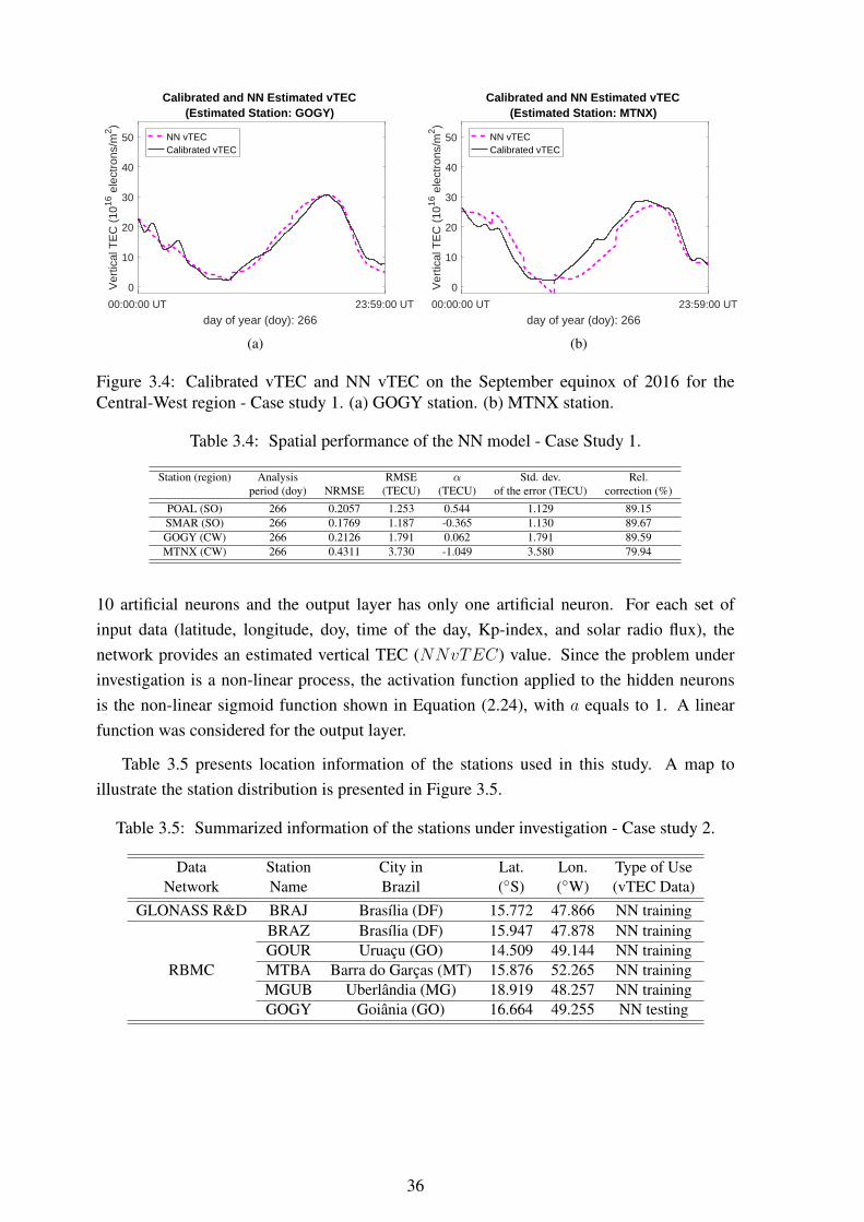
00:00:00 UT 23:59:00 UT

day of year (doy): 266

0

10

20

30

40

50

Ver

tical

TE

C (

1016

ele

ctro

ns/m

2 )Calibrated and NN Estimated vTEC

(Estimated Station: GOGY)

NN vTECCalibrated vTEC

(a)

00:00:00 UT 23:59:00 UT

day of year (doy): 266

0

10

20

30

40

50

Ver

tical

TE

C (

1016

ele

ctro

ns/m

2 )

Calibrated and NN Estimated vTEC(Estimated Station: MTNX)

NN vTECCalibrated vTEC

(b)

Figure 3.4: Calibrated vTEC and NN vTEC on the September equinox of 2016 for theCentral-West region - Case study 1. (a) GOGY station. (b) MTNX station.

Table 3.4: Spatial performance of the NN model - Case Study 1.

Station (region) Analysis RMSE α Std. dev. Rel.period (doy) NRMSE (TECU) (TECU) of the error (TECU) correction (%)

POAL (SO) 266 0.2057 1.253 0.544 1.129 89.15SMAR (SO) 266 0.1769 1.187 -0.365 1.130 89.67GOGY (CW) 266 0.2126 1.791 0.062 1.791 89.59MTNX (CW) 266 0.4311 3.730 -1.049 3.580 79.94

10 artificial neurons and the output layer has only one artificial neuron. For each set ofinput data (latitude, longitude, doy, time of the day, Kp-index, and solar radio flux), thenetwork provides an estimated vertical TEC (NNvTEC) value. Since the problem underinvestigation is a non-linear process, the activation function applied to the hidden neuronsis the non-linear sigmoid function shown in Equation (2.24), with a equals to 1. A linearfunction was considered for the output layer.

Table 3.5 presents location information of the stations used in this study. A map toillustrate the station distribution is presented in Figure 3.5.

Table 3.5: Summarized information of the stations under investigation - Case study 2.

Data Station City in Lat. Lon. Type of UseNetwork Name Brazil (◦S) (◦W) (vTEC Data)

GLONASS R&D BRAJ Brasília (DF) 15.772 47.866 NN training

RBMC

BRAZ Brasília (DF) 15.947 47.878 NN trainingGOUR Uruaçu (GO) 14.509 49.144 NN trainingMTBA Barra do Garças (MT) 15.876 52.265 NN trainingMGUB Uberlândia (MG) 18.919 48.257 NN trainingGOGY Goiânia (GO) 16.664 49.255 NN testing

36

20° W 40° W 60° W 80° W 100° W

20° N

0°

20° S

Figure 3.5: Positions in the world map of the stations under investigation - Case study 2.Green and blue dots represent training and testing station, respectively.

3.3.1 Training the NN

In this scenario, vTEC data from stations GOUR, MTBA, MGUB and BRAJ were usedin the training process. The pair input-output used to train the network consists of an inputvector containing the latitude, longitude, doy, time of the day, Kp-index, and solar radio fluxand the output is the vTEC calculated using the GPS-TEC Analysis Application described inSection 3.1.2. Input-output data from doy 154 to 163 were applied randomly to the networkduring the training process.

Due to the absence of data for some stations in the considered interval, a total of 43200samples were presented to the network during the learning process. In order to avoid overfit-ting or overtraining, 85% of the training set was used to the training procedure and 15% wasused to validate the model. This procedure is important since the network may lose its gener-alization ability if overtrained (HAYKIN, 2009). The Levenberg-Maquardt backpropagationalgorithm was used to set the ANN weights.

Figure 3.6 presents the performance of the ANN for each epoch during the training andvalidation procedures. The best validation performance was obtained at the epoch 159, cor-responding to a Mean Square Error of 2.750 TECU2.

3.3.2 Results and discussions

After the training procedure, the network is then used to estimate the vTEC profile forGOGY station from doy 154 to 163. Figure 3.7 presents the vTEC estimated by the ANNand the vTEC calculated using the GPS-TEC Analysis Application for the GOGY station.

Table 3.6 summarizes some statistics of the results obtained with the proposed ANN

37

0 20 40 60 80 100 120 140 160

Epoch

100

102

Mea

n S

qu

ared

Err

or

(m

se)

Training and validation performance

TrainingValidationBest

Figure 3.6: Performance of the ANN during the training and validation procedures - Casestudy 2.

154 155 156 157 158 159 160 161 162 163

day of year (doy)

0

5

10

15

20

25

30

35

40

45

50

Ver

tical

TE

C (

1016

elec

tron

s/m

2 )

Calibrated and NN estimated vTEC (Estimated Station: GOGY)

NN vTECCalibrated vTEC

Figure 3.7: Calibrated vTEC and NN vTEC on GOGY station - Case Study 2.

model. As shown in Table 3.6, the average error α of the estimative is -0.016 TECU and thestandard deviation of the error is 1.635 TECU. In terms of relative error ε, it was found anaverage value of 11.19%. Alternatively, indicating an agreement in 88.81% of the cases onaverage.

Table 3.6: Spatial performance of the NN model - Case study 2.

Station (region) Analysis RMSE α Std. dev. Avg. rel.period (doy) NRMSE (TECU) (TECU) of the error (TECU) correction (%)

GOGY (CW) 154 to 163 0.1948 1.635 -0.016 1.635 88.81

3.4 Case study 3

In this Case study, the vTEC values on three distinct Brazilian regions (Northeast,Central-West and South) are estimated. Data from two ten-days periods (from doy 154 to163 and from 282 to 291) are used to train the ANN. By using this dataset, three distinct

38

analyses have been carried out in order to assess time-varying and spatial performance of theANN model.

At the spatial performance analysis, for each region, a set of stations is chosen to providetraining data to the ANN and after the training procedure the ANN is used to estimate vTECvalues for the test station which data were not presented to the ANN during the trainingprocess. An analysis is done by comparing, for each testing station, the estimated NNvTECdelivered by the ANN and the reference calibrated vTEC. As a second analysis, the NNability to forecast one day after the time interval (doy 292) based on information of thesecond period of investigation is also assessed in order to verify the feasibility of using a lowamount of data for short-term forecasting. In a third analysis, the spatial performance of theANN model is assessed and compared against CODE Global Ionospheric Maps during thegeomagnetic storm registered on 13th and 14th October 2016.

3.4.1 Training the NN

Aiming to evaluate the performance of the proposed ANN model, vTEC values of North-east, Central-west and South regions of Brazil are investigated. To accomplish this task, foreach region, a set of stations is selected to provide training data to the ANN and one station(out of the training set) is used to test the network and measure its performance. It is impor-tant to notice that no data from the test station are presented to the ANN during the trainingprocess.

Known input and output data are required to train the network. The input vector consistsof latitude, longitude, doy, time of the day, Kp-index, and solar radio flux, and the output isthe calibrated vTEC using the ICTP calibration technique described in Section 3.1.2.

The map shown in Figure 3.8 presents the positions of the stations under analysis for eachregion. The training and test stations are represented by the green and blue dots, respectively.

Data from two different periods in 2016 are used in the training procedure. The firstand second periods will be referred to as Period A and Period B, respectively. Period Acorresponds to doy 154 to 163 (from June 2nd to June 11th, 2016). Average solar radioflux (10.7 cm) is 84.77 sfu with a standard deviation of 3.59 sfu, for this interval. Period Bcorresponds to doy from 282 to 291 (from October 8th to October 17th, 2016) and presentsan average solar radio flux (10.7 cm) of 94.33 sfu with a standard deviation of 10.06 sfu.

39

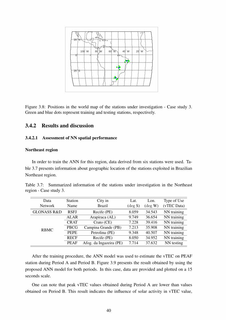
20° W 40° W 60° W 80° W 100° W

20° N

0°

20° S

Figure 3.8: Positions in the world map of the stations under investigation - Case study 3.Green and blue dots represent training and testing stations, respectively.

3.4.2 Results and discussion

3.4.2.1 Assessment of NN spatial performance

Northeast region

In order to train the ANN for this region, data derived from six stations were used. Ta-ble 3.7 presents information about geographic location of the stations exploited in BrazilianNortheast region.

Table 3.7: Summarized information of the stations under investigation in the Northeastregion - Case study 3.

Data Station City in Lat. Lon. Type of UseNetwork Name Brazil (deg S) (deg W) (vTEC Data)

GLONASS R&D RSFJ Recife (PE) 8.059 34.543 NN training

RBMC

ALAR Arapiraca (AL) 9.749 36.654 NN trainingCRAT Crato (CE) 7.228 39.416 NN trainingPBCG Campina Grande (PB) 7.213 35.908 NN trainingPEPE Petrolina (PE) 9.348 40.507 NN trainingRECF Recife (PE) 8.050 34.952 NN trainingPEAF Afog. da Ingazeira (PE) 7.714 37.632 NN testing

After the training procedure, the ANN model was used to estimate the vTEC on PEAFstation during Period A and Period B. Figure 3.9 presents the result obtained by using theproposed ANN model for both periods. In this case, data are provided and plotted on a 15seconds scale.

One can note that peak vTEC values obtained during Period A are lower than valuesobtained on Period B. This result indicates the influence of solar activity in vTEC value,

40

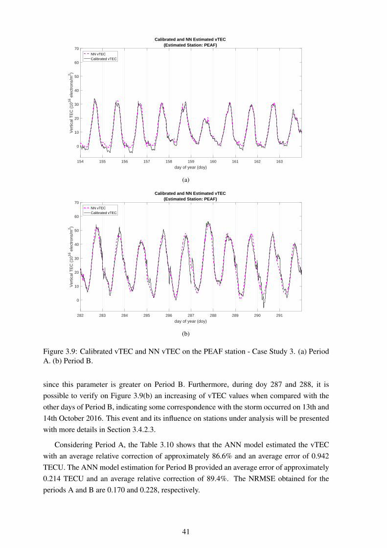
154 155 156 157 158 159 160 161 162 163

day of year (doy)

0

10

20

30

40

50

60

70

Ver

tical

TE

C (

1016

ele

ctro

ns/m

2 )

Calibrated and NN Estimated vTEC(Estimated Station: PEAF)

NN vTECCalibrated vTEC

(a)

282 283 284 285 286 287 288 289 290 291

day of year (doy)

0

10

20

30

40

50

60

70

Ver

tical

TE

C (

1016

ele

ctro

ns/m

2 )

Calibrated and NN Estimated vTEC(Estimated Station: PEAF)

NN vTECCalibrated vTEC

(b)

Figure 3.9: Calibrated vTEC and NN vTEC on the PEAF station - Case Study 3. (a) PeriodA. (b) Period B.

since this parameter is greater on Period B. Furthermore, during doy 287 and 288, it ispossible to verify on Figure 3.9(b) an increasing of vTEC values when compared with theother days of Period B, indicating some correspondence with the storm occurred on 13th and14th October 2016. This event and its influence on stations under analysis will be presentedwith more details in Section 3.4.2.3.

Considering Period A, the Table 3.10 shows that the ANN model estimated the vTECwith an average relative correction of approximately 86.6% and an average error of 0.942TECU. The ANN model estimation for Period B provided an average error of approximately0.214 TECU and an average relative correction of 89.4%. The NRMSE obtained for theperiods A and B are 0.170 and 0.228, respectively.

41

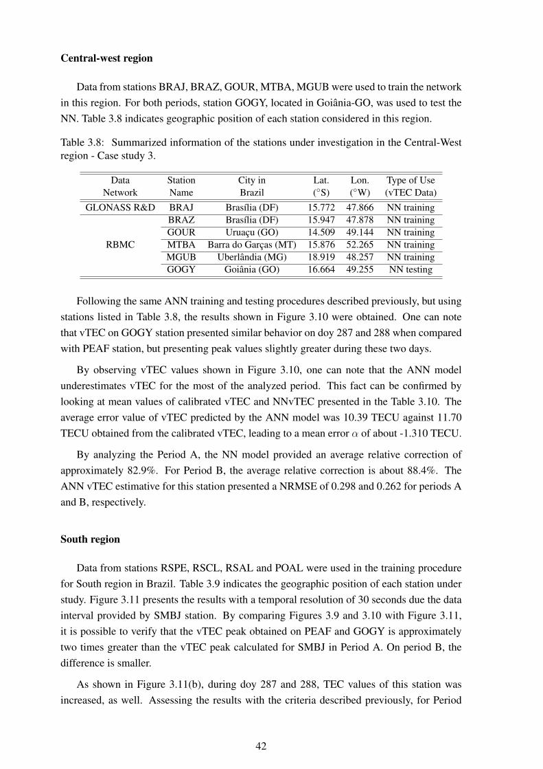
Central-west region

Data from stations BRAJ, BRAZ, GOUR, MTBA, MGUB were used to train the networkin this region. For both periods, station GOGY, located in Goiânia-GO, was used to test theNN. Table 3.8 indicates geographic position of each station considered in this region.

Table 3.8: Summarized information of the stations under investigation in the Central-Westregion - Case study 3.

Data Station City in Lat. Lon. Type of UseNetwork Name Brazil (◦S) (◦W) (vTEC Data)

GLONASS R&D BRAJ Brasília (DF) 15.772 47.866 NN training

RBMC

BRAZ Brasília (DF) 15.947 47.878 NN trainingGOUR Uruaçu (GO) 14.509 49.144 NN trainingMTBA Barra do Garças (MT) 15.876 52.265 NN trainingMGUB Uberlândia (MG) 18.919 48.257 NN trainingGOGY Goiânia (GO) 16.664 49.255 NN testing

Following the same ANN training and testing procedures described previously, but usingstations listed in Table 3.8, the results shown in Figure 3.10 were obtained. One can notethat vTEC on GOGY station presented similar behavior on doy 287 and 288 when comparedwith PEAF station, but presenting peak values slightly greater during these two days.

By observing vTEC values shown in Figure 3.10, one can note that the ANN modelunderestimates vTEC for the most of the analyzed period. This fact can be confirmed bylooking at mean values of calibrated vTEC and NNvTEC presented in the Table 3.10. Theaverage error value of vTEC predicted by the ANN model was 10.39 TECU against 11.70TECU obtained from the calibrated vTEC, leading to a mean error α of about -1.310 TECU.

By analyzing the Period A, the NN model provided an average relative correction ofapproximately 82.9%. For Period B, the average relative correction is about 88.4%. TheANN vTEC estimative for this station presented a NRMSE of 0.298 and 0.262 for periods Aand B, respectively.

South region

Data from stations RSPE, RSCL, RSAL and POAL were used in the training procedurefor South region in Brazil. Table 3.9 indicates the geographic position of each station understudy. Figure 3.11 presents the results with a temporal resolution of 30 seconds due the datainterval provided by SMBJ station. By comparing Figures 3.9 and 3.10 with Figure 3.11,it is possible to verify that the vTEC peak obtained on PEAF and GOGY is approximatelytwo times greater than the vTEC peak calculated for SMBJ in Period A. On period B, thedifference is smaller.

As shown in Figure 3.11(b), during doy 287 and 288, TEC values of this station wasincreased, as well. Assessing the results with the criteria described previously, for Period

42

154 155 156 157 158 159 160 161 162 163

day of year (doy)

0

10

20

30

40

50

60

70

Ver

tical

TE

C (

1016

ele

ctro

ns/m

2 )

Calibrated and NN Estimated vTEC(Estimated Station: GOGY)

NN vTECCalibrated vTEC

(a)

282 283 284 285 286 287 288 289 290 291

day of year (doy)

0

10

20

30

40

50

60

70

Ver

tical

TE

C (

1016

ele

ctro

ns/m

2 )

Calibrated and NN Estimated vTEC(Estimated Station: GOGY)

NN vTECCalibrated vTEC

(b)

Figure 3.10: Calibrated vTEC and NN vTEC on GOGY station - Case study 3. (a) Period A.(b) Period B.

Table 3.9: Summarized information of the stations under investigation in the South region -Case study 3.

Data Station City in Lat. Lon. Type of UseNetwork Name Brazil (◦S) (◦W) (vTEC Data)

GLONASS R&D SMBJ Santa Maria (RS) 29.718 53.719 NN testing

RBMC

RSPE Pelotas (RS) 31.802 52.418 NN trainingRSCL Cerro Largo (RS) 28.141 54.755 NN trainingRSAL Alegrete (RS) 29.789 55.769 NN trainingPOAL Porto Alegre (RS) 30.659 51.120 NN training

A, the ANN model provided an average relative correction of approximately 88.6%. ForPeriod B, the average relative correction obtained is about 88.9%. At this location, the ANN

43

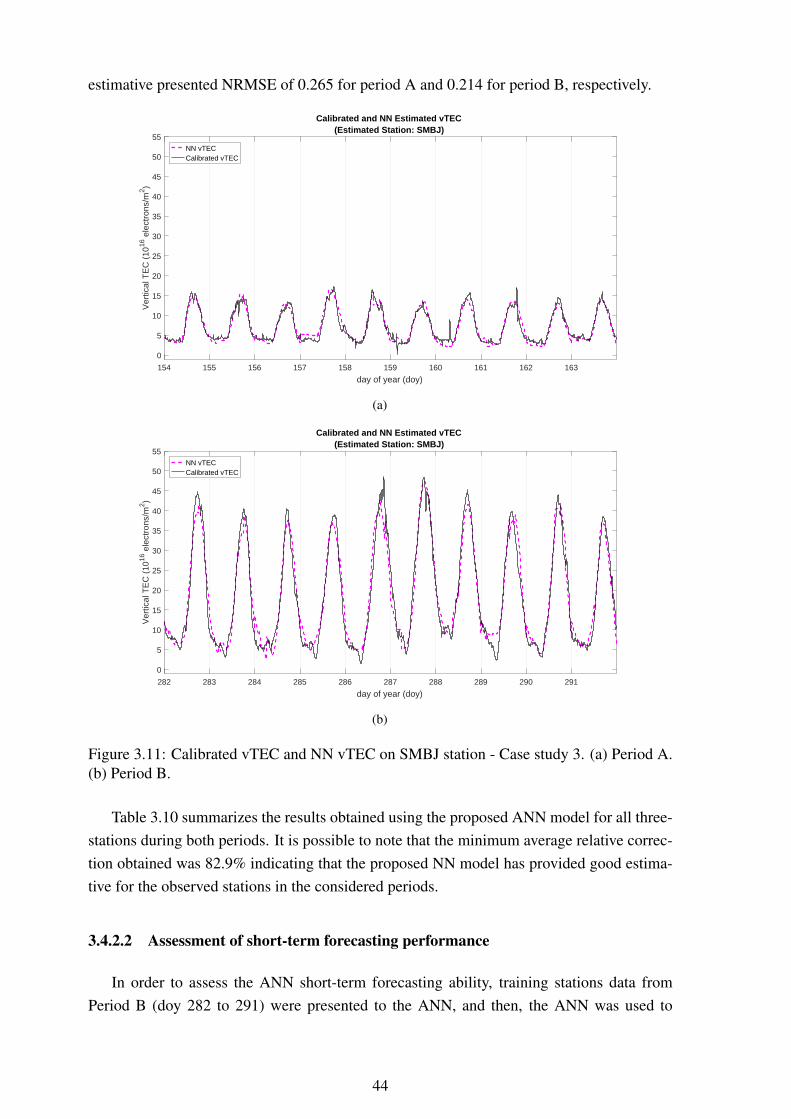
estimative presented NRMSE of 0.265 for period A and 0.214 for period B, respectively.

154 155 156 157 158 159 160 161 162 163

day of year (doy)

0

5

10

15

20

25

30

35

40

45

50

55V

ertic

al T

EC

(10

16 e

lect

rons

/m2 )

Calibrated and NN Estimated vTEC(Estimated Station: SMBJ)

NN vTECCalibrated vTEC

(a)

282 283 284 285 286 287 288 289 290 291

day of year (doy)

0

5

10

15

20

25

30

35

40

45

50

55

Ver

tical

TE

C (

1016

ele

ctro

ns/m

2 )

Calibrated and NN Estimated vTEC(Estimated Station: SMBJ)

NN vTECCalibrated vTEC

(b)

Figure 3.11: Calibrated vTEC and NN vTEC on SMBJ station - Case study 3. (a) Period A.(b) Period B.

Table 3.10 summarizes the results obtained using the proposed ANN model for all three-stations during both periods. It is possible to note that the minimum average relative correc-tion obtained was 82.9% indicating that the proposed NN model has provided good estima-tive for the observed stations in the considered periods.

3.4.2.2 Assessment of short-term forecasting performance

In order to assess the ANN short-term forecasting ability, training stations data fromPeriod B (doy 282 to 291) were presented to the ANN, and then, the ANN was used to

44

Table 3.10: Spatial performance of the NN model - Case study 3.

Station Analysis RMSE α Std. dev. Rel.(region) period NRMSE (TECU) (TECU) of the error (TECU) correction (%)

PEAF A 0.170 1.762 0.942 1.488 86.6(NE) B 0.228 3.401 0.214 3.394 89.4

GOGY A 0.298 2.615 -1.310 2.267 82.9(CW) B 0.261 3.768 0.289 3.757 88.4

SMBJ A 0.265 1.073 0.078 1.070 88.6(SO) B 0.209 2.663 0.239 2.653 88.9

forecast vTEC on doy 292. It is important to highlight that no data from doy 292 werepresented to the ANN in the training procedure. The results for stations PEAF and GOGYare presented on a 30s basis and for SMBJ station the results are presented in a 15s basis.

00:00:00 UT 23:59:45 UT

day of year (doy): 292

0

10

20

30

40

50

Ver

tical

TE

C (

1016

ele

ctro

ns/m

2 )

Calibrated and NN Estimated vTEC(Estimated Station: PEAF)

NN vTECCalibrated vTEC

(a)

00:00:00 UT 23:59:45 UT

day of year (doy): 292

0

10

20

30

40

50V

ertic

al T

EC

(10

16 e

lect

rons

/m2 )

Calibrated and NN Estimated vTEC(Estimated Station: GOGY)

NN vTECCalibrated vTEC

(b)

00:00:00 UT 23:59:30 UT

day of year (doy): 292

0

10

20

30

40

50

Ver

tical

TE

C (

1016

ele

ctro

ns/m

2 )

Calibrated and NN Estimated vTEC(Estimated Station: SMBJ)

NN vTECCalibrated vTEC

(c)

Figure 3.12: Calibrated vTEC and NN vTEC for short-term forescasting of doy 292 - Casestudy 3. (a) PEAF station. (b) GOGY station. (c) SMBJ station.

Table 3.11 presents the results obtained for each region under investigation. One cannote that the maximum RMSE error obtained for short-time forecasting was found at PEAFstation, corresponding to 7.84 TECU. At this station, the average relative correction observedwas 73.5%. Better results were obtained at GOGY and SMBJ stations, with a RMSE of 5.18and 4.05 TECU, respectively.

45

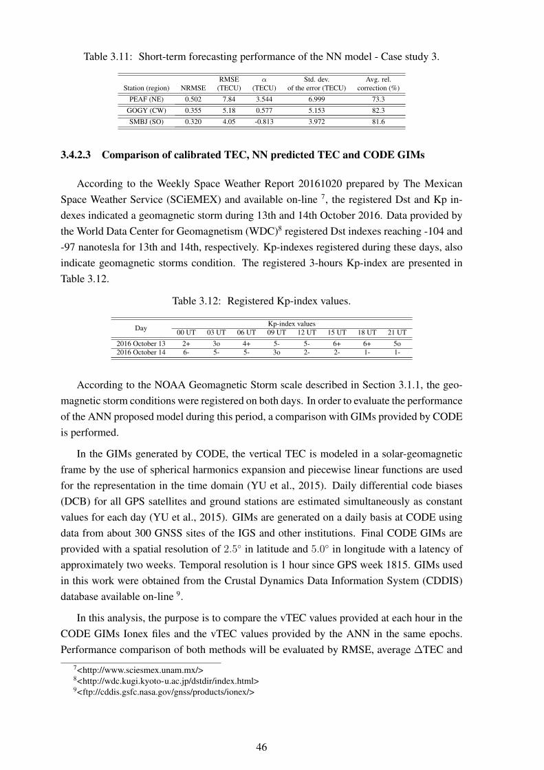
Table 3.11: Short-term forecasting performance of the NN model - Case study 3.

RMSE α Std. dev. Avg. rel.Station (region) NRMSE (TECU) (TECU) of the error (TECU) correction (%)

PEAF (NE) 0.502 7.84 3.544 6.999 73.3

GOGY (CW) 0.355 5.18 0.577 5.153 82.3

SMBJ (SO) 0.320 4.05 -0.813 3.972 81.6

3.4.2.3 Comparison of calibrated TEC, NN predicted TEC and CODE GIMs

According to the Weekly Space Weather Report 20161020 prepared by The MexicanSpace Weather Service (SCiEMEX) and available on-line 7, the registered Dst and Kp in-dexes indicated a geomagnetic storm during 13th and 14th October 2016. Data provided bythe World Data Center for Geomagnetism (WDC)8 registered Dst indexes reaching -104 and-97 nanotesla for 13th and 14th, respectively. Kp-indexes registered during these days, alsoindicate geomagnetic storms condition. The registered 3-hours Kp-index are presented inTable 3.12.

Table 3.12: Registered Kp-index values.

Day Kp-index values00 UT 03 UT 06 UT 09 UT 12 UT 15 UT 18 UT 21 UT

2016 October 13 2+ 3o 4+ 5- 5- 6+ 6+ 5o2016 October 14 6- 5- 5- 3o 2- 2- 1- 1-

According to the NOAA Geomagnetic Storm scale described in Section 3.1.1, the geo-magnetic storm conditions were registered on both days. In order to evaluate the performanceof the ANN proposed model during this period, a comparison with GIMs provided by CODEis performed.

In the GIMs generated by CODE, the vertical TEC is modeled in a solar-geomagneticframe by the use of spherical harmonics expansion and piecewise linear functions are usedfor the representation in the time domain (YU et al., 2015). Daily differential code biases(DCB) for all GPS satellites and ground stations are estimated simultaneously as constantvalues for each day (YU et al., 2015). GIMs are generated on a daily basis at CODE usingdata from about 300 GNSS sites of the IGS and other institutions. Final CODE GIMs areprovided with a spatial resolution of 2.5◦ in latitude and 5.0◦ in longitude with a latency ofapproximately two weeks. Temporal resolution is 1 hour since GPS week 1815. GIMs usedin this work were obtained from the Crustal Dynamics Data Information System (CDDIS)database available on-line 9.

In this analysis, the purpose is to compare the vTEC values provided at each hour in theCODE GIMs Ionex files and the vTEC values provided by the ANN in the same epochs.Performance comparison of both methods will be evaluated by RMSE, average ∆TEC and

7<http://www.sciesmex.unam.mx/>8<http://wdc.kugi.kyoto-u.ac.jp/dstdir/index.html>9<ftp://cddis.gsfc.nasa.gov/gnss/products/ionex/>

46

average relative correction considering calibrated vTEC as the reference. Average ∆Tav isdefined as (HABARULEMA et al., 2009):

∆Tav =1

N

N∑i=1

((Tj=1,2)i − Ti), (3.7)

where ∆Tav is the average difference between the calibrated GNSS vTEC (T ) and NN TEC(Tj=1) or GIM TEC (Tj=2), i = 1, 2, ..., N with N corresponding to the number of observa-tions at a particular time during the interval.

Figure 3.13 presents the calibrated vTEC, NNvTEC and GIM vTEC from doy 286 (0h00UT) to doy 288 (23h00 UT). Calibrated vTEC and NNvTEC data are not available for PEAFstation in 0h00 UT of doy 287, therefore, this observation will not be plotted or consideredin the computation of performance.

286 287 288

day of year (doy)

0

10

20

30

40

50

60

70

Ver

tical

TE

C (

TE

CU

)

Hourly vTEC - PEAF Station

GIM CODEvTECNN vTEC

(a)

286 287 288

day of year (doy)

0

10

20

30

40

50

60

70V

ertic

al T

EC

(T

EC

U)

Hourly vTEC - GOGY Station

GIM CODEvTECNN vTEC

(b)

286 287 288

day of year (doy)

0

10

20

30

40

50

60

70

Ver

tical

TE

C (

TE

CU

)

Hourly vTEC - SMBJ Station

GIM CODEvTECNN vTEC

(c)

Figure 3.13: Calibrated vTEC, NN vTEC, and GIM derived vTEC from doy 286 to 288 onyear 2016 - Case study 3. (a) PEAF station. (b) GOGY station. (c) SMBJ station.

As shown in Figure 3.13, the proposed NN presented better results when compared withCODE GIMs during the period under investigation (considering vTEC provided by the cali-bration as the reference). In almost all period, GIMs overestimate TEC values in all stations.

47

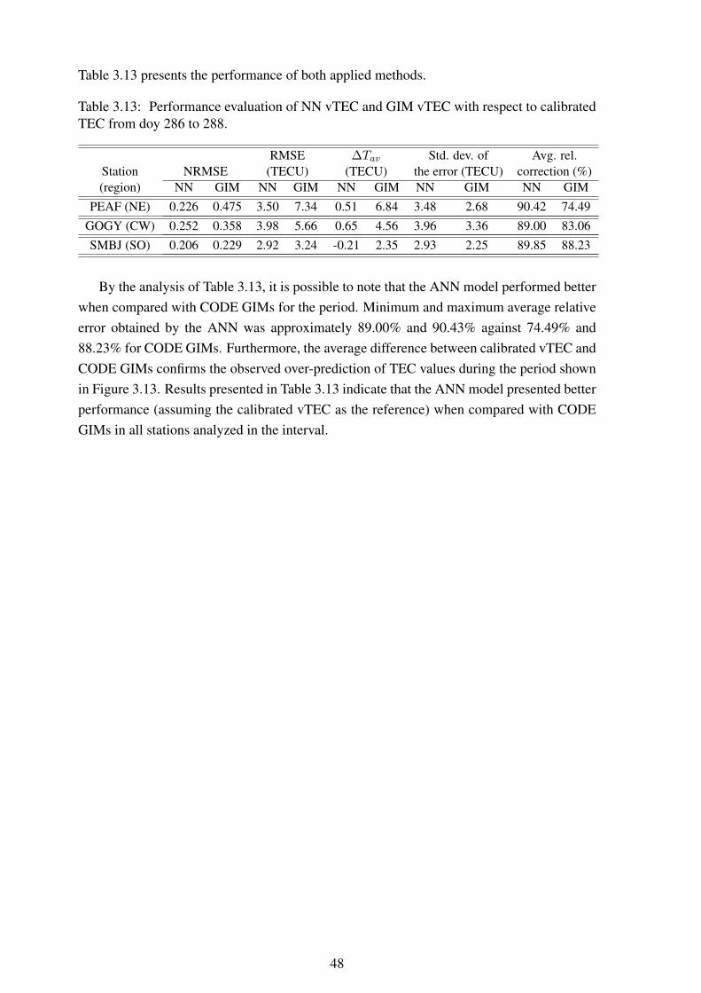
Table 3.13 presents the performance of both applied methods.

Table 3.13: Performance evaluation of NN vTEC and GIM vTEC with respect to calibratedTEC from doy 286 to 288.

RMSE ∆Tav Std. dev. of Avg. rel.Station NRMSE (TECU) (TECU) the error (TECU) correction (%)(region) NN GIM NN GIM NN GIM NN GIM NN GIM

PEAF (NE) 0.226 0.475 3.50 7.34 0.51 6.84 3.48 2.68 90.42 74.49GOGY (CW) 0.252 0.358 3.98 5.66 0.65 4.56 3.96 3.36 89.00 83.06SMBJ (SO) 0.206 0.229 2.92 3.24 -0.21 2.35 2.93 2.25 89.85 88.23

By the analysis of Table 3.13, it is possible to note that the ANN model performed betterwhen compared with CODE GIMs for the period. Minimum and maximum average relativeerror obtained by the ANN was approximately 89.00% and 90.43% against 74.49% and88.23% for CODE GIMs. Furthermore, the average difference between calibrated vTEC andCODE GIMs confirms the observed over-prediction of TEC values during the period shownin Figure 3.13. Results presented in Table 3.13 indicate that the ANN model presented betterperformance (assuming the calibrated vTEC as the reference) when compared with CODEGIMs in all stations analyzed in the interval.

48

Chapter 4

Conclusion

The results obtained by the analysis performed in the cases of study presented in thiswork indicate that the use of the proposed Artificial Neural Network models for verticalTEC estimation can provide good estimates in the Brazilian region. The studies performedin the case study 1 presented the impact of choosing different parameters to compose theANN model. For this case study, the use of the Kp-index and the solar radio flux presentedbetter results. Also, it was possible to note that the number of neurons employed in theANN is an important parameter to be considered. A large number of neurons does not leadnecessarily to a performance improvement for the investigated ANNs. For the case study2, the proposed ANN model has provided an average relative correction of 88.81% and aRMSE value of 1.635 TECU.

Considering the case study 3, one can verify that the proposed model has provided aminimum relative correction value of approximately 82.9% and a maximum RMSE of 3.76TECU. Periods of higher solar activity presented the worst average absolute errors results.Periods of lower solar activity provided worst relative error results, due to the lower absoluteTEC during days with low solar activities. By analyzing the average absolute error of theANN model it is possible to verify that better results were obtained during the lower solaractivity period.

In the forecasting performance analysis presented in the case study 3, the maximumRMSE value obtained was 7.84 TECU at PEAF station. Best results were obtained forGOGY and SMBJ stations, reaching RMSE values of 5.18 and 4.05 TECU, respectively.The obtained estimation suggests that the proposed ANN can be exploited on the develop-ment of a TEC short-term prediction model in Brazil. Future studies will be carried out inorder to determine the suitable training interval to obtain minimum error values in short-termforecasting and improve the NN performance in the regions located at lower latitudes. Also,the use of recurrent ANNs will be investigated.

Investigation of performance during the period from DoY 286 to 288 shows that the ANNmodel provided better results when compared with CODE GIMs, assuming the calibrated

49

vTEC as the reference. Performance assessed by this work suggests that the proposed ANNmodel is a promising tool for vTEC estimation in void areas even during events such asthe geomagnetic storm registered during 13th and 14th October 2016. It is important tonote that work does not intend to undervalue the estimations provided by CODE GlobalIonospheric Model, but rather, reinforce its important role in studies and improvements ofregional models.

It is worth mentioning that the proposed ANN model does not have the ability to calibratevTEC by itself, relying on data provided by the calibration technique. Therefore, if vTECdelivered by the calibration procedure present negative values, the ANN can incorporate thisresults, and as a consequence presents negative vTEC.

The studies presented in this manuscript were the basis for the investigations publishedin three papers. The list of publications derived from this research can be found in AppendixA. In future works, the investigations on the development of a model that includes the fiveBrazilian regions can be performed. The applicability in short-term forecasting in a nearreal-time scenario will also be investigated. In addition, the performance analysis of low-cost single-frequency receivers using the TEC values from the proposed ANN to mitigatethe ionospheric range error in positioning systems will also be investigated.

50

REFERENCES

AGUIAR, C. R. Modelo Regional da Ionosfera Mod ion: implementação em tempo real.Master Thesis (MSc) — Faculdade de Ciências e Tecnologia UNESP, Presidente Prudente,2005.

ALKAN, R. M.; KAMMAN, H.; SAHIN, M. GPS, GALILEO and GLONASS SatelliteNavigation Systems & GPS Modernization. In: IEEE. Proceedings of 2nd InternationalConference on Recent Advances in Space Technologies. Istanbul, Turkey, 2005. p. 390–394.

APPLETON, E. V. Wireless studies of the ionosphere. In: INSTITUTION OF ELECTRI-CAL ENGINEERS. Journal of the Institution of Electrical Engineers. 1932. v. 71, no. 430,p. 642–650.

ARBESSER-RASTBURG, B.; ROGERS, D. Earth–space propagation. In: BARCLAY, L.(Ed.). Propagation of Radio Waves. 3rd. ed. : The Institution of Engineering and Technology,2013. p. 335–363.

BARTELS, J. III - The geomagnetic measures for the time-variations of solar corpuscularradiation, described for use in correlation studies in other geophysical fields. In: INTERNA-TIONALE, C. I. C. of Scientific Unions Comité Spécial de lÁnnée G. (Ed.). Geomagnetism.: Pergamon, 1957, (Annals of The International Geophysical Year, v. 4). p. 227–236.

BHUYAN, P. K.; BORAH, R. R. TEC derived from GPS network in India and comparisonwith the IRI. Advances in Space Research, v. 39, no. 5, p. 830–840, 2007.

BISHOP, G. J.; KLOBUCHAR, J. A.; DOHERTY, P. H. Multipath effects on the determi-nation of absolue ionospheric time delay from GPS signals. Radio Science, v. 20, no. 3, p.388–396, May-June 1985.

BORRE, K. et al. A Software-Designed and GPS Galileo Receiver - A Single-FrequencyApproach. : Birkhäuser Boston, 2007.

BORRE, K.; STRANG, G. Algorithms for global positioning. Wellesey MA USA: Cam-bridge University Press, 2012. 450 p.

BRAASCH, M. S. Multipath effects. In: PARKINSON, B. W.; JR., J. J. S. (Ed.). GlobalPositioning Systems: Theory and Applications. : American Institute of Aeronautics and As-tronautics, 1996, (Progress in Astronautics and Aeronautics, v. 1). ch. 14, p. 547–568.

BREE, R. J. P. van; TIBERIUS, C. C. J. M. Real-time single-frequency precise point posi-tioning: accuracy assessment. GPS Solutions, v. 16, no. 2, p. 259–266, April 2012.

CESARONI, C. et al. L-band scintillations and calibrated total electron content gradientsover Brazil during the last solar maximum. Journal of Space Weather and Space Climate,v. 5, no. A36, p. 1–11, December 2015.

51

CIRAOLO, L. et al. Calibration errors on experimental slant total electron content (TEC)determined with GPS. Journal of Geodesy, v. 81, p. 111–120, February 2007.

CLOSAS, P.; FERNÁNDEZ-PRADES, C.; FERNÁNDEZ-RUBIO, J. A. A bayesian ap-proach to multipath mitigation in gnss receivers. IEEE Journal of Selected Topics in SignalProcessing, v. 3, no. 4, p. 695–706, August 2009.

CONKER, R. S. et al. Modeling the effects of ionospheric scintillation on GPS/Satellite-Based Augmentation System availability. Radio Science, v. 38, no. 1, p. 1–23, January 2003.

CYBENKO, G. Approximation by superpositions of a sigmoidal function. Math. ControlSignals Systems, v. 2, p. 303–314, 1989.

DENARDINI, C. M.; DASSOB, S.; G.-ESPARZAD, J. A. Review on space weather in LatinAmerica. 2. the research networks ready for space weather. Advances in Space Research,v. 58, no. 10, p. 1940–1959, March 2016.

DENARDINI, C. M.; DASSOB, S.; G.-ESPARZAD, J. A. Review on space weather in LatinAmerica. 3. Development of space weather forecasting centers. Advances in Space Research,v. 58, no. 10, p. 1960–1967, March 2016.

DoD. Interface Specification IS-GPS-200: Navstar GPS Space Segment/Navigation UserInterfaces. 2012.

DoD, USA. Global Positionig System Standard Positioning Service Signal Specification.2nd. ed. June 1995.

DYRUD, L. et al. Ionospheric measurement with GPS: receiver techniques and methods.Radio Science, v. 43, no. 6, p. 1–11, December 2008.

EL-HATTAB, A. I. Influence of GPS antenna phase center variation on precise positioning.NRIAG Journal of Astronomy and Geophysics, v. 2, no. 2, p. 272–277, December 2013.

ELMAS, Z. G. et al. Higher order ionospheric effects in GNSS positioning in the europeanregion. Annales Geophysicae, v. 29, p. 1383–1399, August 2011.

ELSOBEIEY, M.; AL-HARBI, S. Performance of real-time Precise Point Positioning usingIGS real-time service. GPS Solutions, v. 20, no. 3, p. 565–571, July 2015.

European Space Agency. <http://www.esa.int/Our_Activities/Navigation/Galileo/What_is_Galileo>. December 2017. Galileo web page.

GLONASS information and Analysis Center. https://www.glonass-iac.ru/en/GLONASS/.December 2017. Official Website.

HABARULEMA, J. B.; MCKINNELL, L.-A.; CILLIERS, P. J. Prediction of global posi-tioning system total electron content using neural networks over South Africa. Journal ofAtmospheric and Solar-Terrestrial Physics, v. 69, p. 1842–1850, September 2007.

HABARULEMA, J. B. et al. Application of neural networks to South African GPS TECmodelling. Advances in Space Research, v. 43, no. 11, p. 1711–1720, June 2009.

HADAS, T. et al. Near-real-time regional troposphere models for the GNSS precise pointpositioning technique. Measurement Science and Technology, v. 24, no. 5, p. 1–12, 2013.

52

HARTMANN, G. K.; LEITINGER, R. Range errors due to ionospheric and troposphericeffects for signal frequencies above 100 MHz. Bulletin Geodesique, v. 58, no. 2, p. 109–136,June 1984.

HAYKIN, S. Neural Networks: A Comprehensive Foundation. 2nd. ed. : Prentice Hall, 1999.

HAYKIN, S. Neural Networks and Learning Machines. 3rd. ed. Bangladesh India: Pearson,2009. 906 p.

HOFMANN-WELLENHOF, B.; LICTHENEGGER, H.; WASLE, E. GNSS - Global Navi-gation Satellite Systems: GPS, GLONASS, Galileo & more. : SpringerWienNewYork, 2008.516 p.

HOQUE, M. M.; JAKOWSKI, N. Ionospheric propagation effects on GNSS signals and newcorrection approaches. In: JIN, S. (Ed.). Global Navigation Satellite Systems: Signal, Theoryand Applications. : InTech, 2012. p. 381–404.

HOQUE, M. M.; JAKOWSKI, N. An alternative ionospheric correction model for GlobalNavigation Satellite Systems. Journal of Geodesy, v. 89, no. 4, p. 391–406, April 2015.

JAKOWSKI, N. et al. Total electron content models and their use in ionosphere monitoring.Radio Science, v. 46, no. 6, p. 1–11, December 2011.

JIN, R.; JIN, S.; FENG, G. M DCB: Matlab code for estimating GNSS satellite and receiverdifferential code biases. GPS Solutions, v. 16, p. 541–548, July 2012.

KAPLAN, E. D.; HEGARTY, C. J. Understanding GPS : Principles and Applications. 2nd.ed. : Artech House, 2006.

KLOBUCHAR, J. A. Ionospheric time-delay algorithm for single-frequency GPS users.IEEE Transactions on Aerospace and Electronic Systems, AES-23, no. 3, May 1987.

KLOBUCHAR, J. A. Ionospheric effects on gps. In: JR., J. J. S. et al. (Ed.). Global Position-ing System: Theory and Applications. : American Institute of Aeronautics and Astronautics,1996, (Progress in Astronautics and Aeronautics, v. 1). ch. 12, p. 485–515.

LANGLEY, R. B. The effect of the ionosphere and troposphere on satellite positioning sys-tems. Proceedings of Symposium on Refraction of Transatmospheric Signals in Geodesy,J.C. de Munck, and T.A. Spoelstra (Eds.) Netherlands Geodetic Commission, Publicationson Geodesy, New Series No. 36, The Hague, The Netherlands,(abstract). The paper is avail-able on the University of New Brunswick Web server, p. 97, May 1992.

LANGLEY, R. B. GPS receivers and the observables. In: KLEUSBERG, A.; TEUNISSEN,P. J. G. (Ed.). GPS for Geodesy. : Springer-Verlag, 1996. p. 141–173.

LEANDRO, R. F.; SANTOS, M. C. A neural network approach for regional vertical totalelectron content modelling. Studia Geophysica et Geodaetica, v. 51, no. 2, p. 279–292, April2007.

LIU, Z. et al. Influence of higher-order ionospheric delay correction on GPS precise orbitdetermination and precise positioning. Geodesy and Geodynamics, v. 7, no. 5, p. 369–376,May 2016.

53

MACHADO, W. C. Utilização de redes neurais artificiais na previsão do VTEC visando ageração de estações de referência virtuais em tempo real. Thesis (PhD) — Escola Politécnicada Universidade de São Paulo, 2012.

MANUCCI, A. J. et al. A global mapping technique for GPS-derived ionospheric total elec-tron content measurements. Radio Science, v. 33, no. 3, p. 565–582, May 1998.

MARINI, J. W. Correction of satellite tracking data for an arbitrary tropospheric profile.Radio Science, v. 7, p. 223–231, February 1972.

MARTINS, S. A. M.; NEPOMUCENO, E. G.; BARROSO, M. F. S. Improved structuredetection for polynomial NARX models using a multiobjective error reduction ratio. Journalof Control, Automation and Electrical Systems, v. 24, no. 6, p. 764–772, September 2013.

MITCHELL, C. The ionosphere. In: BARCLAY, L. (Ed.). Propagation of Radio Waves. 3rd.ed. : The Institution of Engineering and Technology, 2013. ch. 11, p. 187–198.

MöLLER, G.; WEBER, R.; BöHM, J. Improved troposphere blind models based on numeri-cal weather data. Navigation: Journal of the Institute of Navigation, v. 61, no. 3, p. 203–211,2014.

MONICO, J. F. G. Posicionamento pelo GNSS: descrição, fundamentos e aplicações (GNSSpositoning: description, fundamentals and applications). 2nd. ed. : Editora Unesp, 2008.476 p.

M.ROTHACHER; G.BEUTLER. The role of GPS in the study of global change. Physicsand Chemistry of the Earth, v. 23, no. 9-10, p. 1029–1040, 1998.

MYLNIKOVA, A. A. et al. Variability of GPS/GLONASS diffrential code biases. Results inPhysics, v. 5, p. 9–10, December 2014.

NIE, Z. et al. An approach to GPS clock prediction for real-time PPP during outages of RTSstream. GPS Solutions, v. 22, p. 1–14, January 2018.

Novatel Inc. An introduction to GNSS - GPS, GLONASS, BeiDou, Galileo and other GlobalNavigation Satellite Systems. 2nd. ed. Calgary, Alberta, CA: Novatel Inc., 2015.

OKOH, D. et al. A regional GNSS-VTEC model over Nigeria using neural networks: Anovel approach. Geodesy and Geodynamics, v. 7, no. 1, p. 19–31, April 2016.

PAPARINI, C. et al. Investigation on the performance of a low-cost single frequency gnssreceiver for PPP application. In: Proceedings of the 19th International Beacon Satellite Sym-posium. 2016. p. 3.

ROCHA, G. D. C.; MARQUES, H. A.; GALERA, J. G. M. Acurácia do posicionamentoabsoluto GPS com correção da ionosfera advinda de mapas ionosféricos globais e reginais.BCG Boletim de Ciências Geodésicas, v. 21, no. 3, p. 498–514, 2015.

ROCHA, R. S. M. et al. Avaliação do efeito da cintilação ionosférica e de diferentes interva-los de tempo de coleta de dados no posicionamento por ponto preciso na sua forma on-line.Revista Brasileira de Geomática, v. 5, no. 2, p. 251–276, 2017.

SAPUCCI, L. F. Estimativa do vapor d’água atmosférico e avaliação da modelagem doatraso zenital troposférico utiizando GPS. Master Thesis (MSc) — Faculdade de Ciências eTecnologia UNESP, 2001.

54

SEEBER, G. Satellite Geodesy. 2nd. ed. : Walter de Gruyter GmbH & Co., 2003.

SEEMALA, G. K. GPS-TEC analysis application. 2017.

SPILKER, J. J. Troposheric effects on GPS. Global Positioning System: Theory and Appli-cations, v. 1, p. 517–546, 1996.

TAKAHASHI, H. et al. Diagnostics of equatorial and low latitude ionosphere by TEC map-ping over Brazil. Advances in Space Research, v. 54, no. 3, p. 385–394, August 2014.

TAPPING, K. F. The 10.7 cm solar radio flux (f10.7). Space Weather, v. 11, p. 394–406, July2013.

TEUNISSEN, P. J. G.; KLEUSBERG, A. Propagation of the GPS signals. In: KLEUS-BERG, A.; TEUNISSEN, P. J. G. (Ed.). GPS for Geodesy. : Springer-Verlag, 1996. p. 174–217.

The European Comission. Open Service signal-in-space interface control document. Decem-ber 2016.

TIWARI, R. et al. WBMod assisted PLL GPS software receiver for mitigating scintillationaffect in high latitude region. In: INTERNATIONAL UNION OF RADIO SCIENCE. 2011XXXth URSI General Assembly and Scientific Symposium. Istanbul, 2011. p. 1–4.

US Department of Defense. https://www.gps.gov/systems/gps/space/. 2017. Official GPSweb-site.

WEBSTER, I. R. A Regional Model for the Prediciton of Ionpspheric Delay for Single Fre-quency Users of the Global Positioning System. Fredericton, New Brunswick, Canada, 1993.

WEINBACH, U.; SCHöN, S. GNSS receiver clock modeling when using high-precisionoscillators and its impact on PPP. Advances in Space Research, v. 47, no. 2, p. 229–238,January 2011.

WILLISCROFT, L. A.; POOLE, A. W. V. Neural networks, foF2, sunspot number and mag-netic activity. Geophysical Research Letters, v. 23, no. 24, p. 3659–3662, December 1996.

YAO, Y. et al. ITG: A new GLobal GNSS Tropospheric Correction Model. Scientific Reports,v. 5, no. 10273, July 2015.

YIBIN, Y. et al. A global empirical model for estimating zenith tropospheric delay. ScienceChina Earth Sciences, v. 59, no. 1, p. 118–128, January 2016.

YU, X. et al. Ionospheric correction based on ingestion of global ionospheric maps into theNequick 2 model. The Scientific World Journal, v. 2015, no. 376702, 2015.

ZHAO, J.; HAN, Y. B. Historical dataset reconstruction and a prediction method of solar10.7 cm radio flux. Chinese Journal of Astronomy and Astrophysics, v. 8, no. 4, p. 472–476,January 2008.

55

Appendices

56

Appendix A

List of publications

A.1 Directly related publications

FERREIRA. A. A.; BORGES, R. A.; PAPARINI, C.; CIRAOLO, L.; RADICELLA, S.M.; Short-term estimation of GNSS TEC using a neural network model in Brazil. Advancesin Space Research, v. 60, p. 1765-1776, 2017.

FERREIRA, A. A.; BORGES, R. A.; PAPARINI, C.; RADICELLA, S.; TEC modellingvia neural network using observations from the first GLONASS R&D data network in Braziland the RBMC. Proceedings of the 20th World Congress of the International Federation ofAutomatic Control (IFAC), Toulouse, 2017. p. 13371-13376.

FERREIRA, A. A.; BORGES, R. A.; Análise de diferentes estruturas de redes neu-rais artificiais Multilayer Perceptron na modelagem do conteúdo total de elétrons.(Analysisof different structures of Multilayer Perceptron artificial neural networks in the modellingof the Total Electron Content.) Presented at the XIII Brazilian Symposium on IntelligentAutomation, 2017 (in Portuguese).

A.2 Indirectly related publications

PAUL, A.; KASCHEYEV, A.; RODRIGUEZ-BOUZA, M.; PATHAK, K.; FERREIRA,A.A.; SHETTI, D.; YAO, J.N. Latitudinal features of Total Electron Content over the Africanand European longitude sector following the St. Patrick’s day storm of 2015. Advances inSpace Research, 2017 (in press).

57

Appendix B

Linearization of the observable equation

By using the ephemeris sent in the navigation message it is possible to obtain the satellitepositioning coordinates (Xsv, Y sv, Zsv) and the satellite clock bias dtsv. The terms corre-sponding to ionospheric and tropospheric delays (T svr e Isvr ) can be obtained from a priorimodels (BORRE et al., 2007). Some strategies to deal with multipath effect (dmsv

r ) arepresented in Section 2.3.2. Thus, the unknowns of Equation (2.5) are the receiver positioncoordinates (Xr, Yr, Zr) and the receiver clock bias.

Since Equation (2.5) is non-linear with respect to the coordinates of the receivers andsatellites, it has to be linearized before applying the least-squares method (BORRE et al.,2007). Considering the non-linear term of the Equation (2.5) it follows, for an epoch t:

ρsvr (t) =

√(Xsv(t)−Xr)

2 + (Y sv(t)− Yr)2 + (Zsv(t)− Zr)2. (B.1)

By assuming the approximated values (Xr,0, Yr,0, Zr,0) for the coordinates of the receiver(station) r, an approximated distance can be obtained by:

ρsvr (t) =

√(Xsv(t)−Xr,0)2 + (Y sv(t)− Yr,0)2 + (Zsv(t)− Zr,0)2, (B.2)

and the coordinates of the station can be represented by:

Xr =Xr,0 + ∆Xr

Yr =Yr,0 + ∆Yr ,

Zr =Zr,0 + ∆Zr

(B.3)

where ∆Xr, ∆Yr and ∆Zr correspond to the corrections to the approximated values (MON-ICO, 2008). This initial approximated coordinate is often chosen as the center of the Earthin the ECEF coordinate system (0,0,0) (BORRE et al., 2007). By applying (B.3) in (B.2) and

58

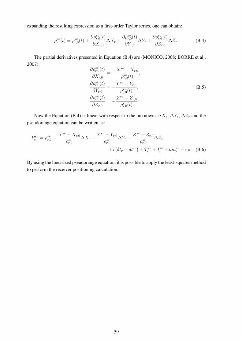
expanding the resulting expression as a first-order Taylor series, one can obtain:

ρsvr (t) = ρsvr,0(t) +∂ρsvr,0(t)

∂Xr,0

∆Xr +∂ρsvr,0(t)

∂Yr,0∆Yr +

∂ρsvr,0(t)

∂Zr,0∆Zr. (B.4)

The partial derivatives presented in Equation (B.4) are (MONICO, 2008; BORRE et al.,2007):

∂ρsvr,0(t)

∂Xr,0

= −Xsv −Xr,0

ρsvr,0(t),

∂ρsvr,0(t)

∂Yr,0= −Y

sv − Yr,0ρsvr,0(t)

,

∂ρsvr,0(t)

∂Zr,0= −Z

sv − Zr,0ρsvr,0(t)

.

(B.5)

Now the Equation (B.4) is linear with respect to the unknowns ∆Xr, ∆Yr, ∆Zr and thepseudorange equation can be written as:

P svr = ρsvr,0 −

Xsv −Xr,0

ρsvr,0∆Xr −

Y sv − Yr,0ρsvr,0

∆Yr −Zsv − Zr,0

ρsvr,0∆Zr

+ c(δtr − δtsv) + T svr + Isvr + dmsvr + εP . (B.6)

By using the linearized pseudorange equation, it is possible to apply the least-squares methodto perform the receiver positioning calculation.

59

Appendix C

Additional tropospheric effectinformation

C.1 Tropospheric attenuation as a function of the elevationangle

By modelling the troposphere as a simple and uniform spherical shell of height hm abovethe Earth, the length of the signal path L through the troposphere varies with the elevationangle (ε) and is given by (SPILKER, 1996)

L =2hm(1 + a/2)

sin(ε) +√sin2(ε) + 2a+ a2

(C.1)

where hm = 6 km, Re corresponds to the Earth radius (Re ≈ 6378 km) and a = hm/Re.Figure C.1 illustrates the length L of signal path in which cos(ε) = (1 + a)cos(φ).

Troposphere

hm

Earth RadiusRe

Earth Center

Length L of path through troposphere

Figure C.1: Path length L through an uniform shell troposphere at elevation angle ε(SPILKER, 1996) (adapted).

60

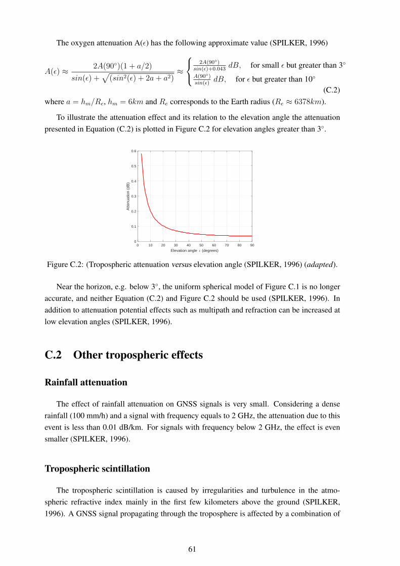
The oxygen attenuation A(ε) has the following approximate value (SPILKER, 1996)

A(ε) ≈ 2A(90◦)(1 + a/2)

sin(ε) +√

(sin2(ε) + 2a+ a2)≈

2A(90◦)

sin(ε)+0.043dB, for small ε but greater than 3◦

A(90◦)sin(ε)

dB, for ε but greater than 10◦

(C.2)where a = hm/Re, hm = 6km and Re corresponds to the Earth radius (Re ≈ 6378km).

To illustrate the attenuation effect and its relation to the elevation angle the attenuationpresented in Equation (C.2) is plotted in Figure C.2 for elevation angles greater than 3◦.

0 10 20 30 40 50 60 70 80 90

Elevation angle ǫ (degrees)

0

0.1

0.2

0.3

0.4

0.5

0.6

Atte

nuat

ion

(dB

)

Figure C.2: (Tropospheric attenuation versus elevation angle (SPILKER, 1996) (adapted).

Near the horizon, e.g. below 3◦, the uniform spherical model of Figure C.1 is no longeraccurate, and neither Equation (C.2) and Figure C.2 should be used (SPILKER, 1996). Inaddition to attenuation potential effects such as multipath and refraction can be increased atlow elevation angles (SPILKER, 1996).

C.2 Other tropospheric effects

Rainfall attenuation

The effect of rainfall attenuation on GNSS signals is very small. Considering a denserainfall (100 mm/h) and a signal with frequency equals to 2 GHz, the attenuation due to thisevent is less than 0.01 dB/km. For signals with frequency below 2 GHz, the effect is evensmaller (SPILKER, 1996).

Tropospheric scintillation

The tropospheric scintillation is caused by irregularities and turbulence in the atmo-spheric refractive index mainly in the first few kilometers above the ground (SPILKER,1996). A GNSS signal propagating through the troposphere is affected by a combination of

61

random absorption and scattering. These effects cause variations in the amplitude and phasein the received waveform (MONICO, 2008; SPILKER, 1996). Tropospheric scintillationeffect varies with time and depends on signal frequency, elevation angle, and weather con-ditions, particularly dense clouds. For elevation angles higher than 10◦ the most significanteffect is the scattering caused by the turbulence. In general, for GNSS signals these effectsare small, except for lower elevation angles (SPILKER, 1996; MONICO, 2008).

C.3 Empirical models and mapping functions

The empirical models for tropospheric delay are functions of meteorological parameters,such as temperature, pressure and humidity. These parameters allow determining the ZenithTroposphere Delay (ZTD), which is mapped into Slant Tropospheric Delay (STD) by usingthe mapping functions (HADAS et al., 2013).

As presented in Section 2.3.3.2 it is necessary to obtain the refractivity index NT alongthe path between the receiver and the satellite to calculate the tropospheric delay from Equa-tion (2.10). The empiric general expression for the refractivity of a non-ideal gas, includingwater vapor, is given by (MONICO, 2008):

NT = k1PhTZ−1H + k2

e

TZ−1W + k3

e

T 2Z−1W (C.3)

where:

• Ph and e are the partial pressure of the dry air and water vapor (expressed in milibars);

• T is the temperature expressed in Kelvin;

• ZW and ZH corresponds to the compressibility factors for the wet and hydrostaticcomponents, respectively;

• the constants k1, k3 e k3 are obtained experimentally with k1 = 77.604 ± 0.0124,k2 = 64.79± 10 and k3 = 377600± 3000.

By using the gases law, one can obtain the following expressions for the hydrostatic andwet refractivities,

NH =k1R

MH

ρ = 22.276ρ, (C.4)

NW =

[k2 − k1

MW

MH

]e

TZ−1W + k3

e

T 2Z−1W . (C.5)

The hydrostatic refractivity presents a low uncertainty (±0.014%) and depends only on thetotal density of the atmosphere, therefore it can be determined with good precision. The wetrefractivity, on the other hand, presents considerable uncertainty in its coefficients. This factdifficults the NW determination (MONICO, 2008).

62

Since the refractivity along the way between the receiver antenna and the satellite is verycomplicated to obtain, several models have been developed to perform a priori corrections ofthe tropospheric delay. In these models, additional parameters can be included in the form ofadjustment parameters. Some common models employed on tropospheric delay correctionare the Hopfield model and Standard Model.

A brief description of these models are as follows:

a) Hopfield model: Among the most knowns models for tropospheric delay, this modelwas developed in the decade of 1960 and is given by the following set of equations:

T sr = TZH ×mh(ε) + TZW ×mw(ε)

TZH = 155.2× 10−7P

THd

TZW = 155.2× 10−7 4819e

T 2Hw

mh(ε) =1√

ε2 + 6.25

mw(ε) =1√

ε2 + 2.25

Hd = 40136 + 148.72(T − 273.16)

Hw = 11000 m

(C.6)

where, the terms TZH , TZW , mh(ε) e mw(ε) are the zenith tropospheric componentsand the mapping functions described previously in Section (2.3.3.2), and ε is the ele-vation angle. Other mapping functions can also be employed.

b) Saastamoinen model: In this model, it is assumed a linear decreasing in the temper-ature until tropopause (about 12 km height); for higher altitudes the stratosphere ischaracterized as an isothermal model by a constant value. Other assumptions weremade in order to develop this model, such as: i) atmosphere in hydrostatic equilib-rium, ii) the water vapor is concentrated in the troposphere and behaves as an idealgas. The standard model proposed by Saastamoinen 1972, with some adjustments, isgiven by (MONICO, 2008; SPILKER, 1996):

T sr = 0.0022771

1 +D

1

cosz

[P +

(1255

T+ 0.05

)e−Btan2z

]+ ∂R, (C.7)

where P and e represent the superficial pressure (expressed in mBar) of dry air andwater vapor, respectively; T is the temperature in Kelvin; B and ∂R are correctionfactors and z = 90◦ − ε. The values of B and ∂R for various users heights can befound in Spilker 1996. The value D is obtained by

D = 0.0026cos(2φ) + 0.00028H, (C.8)

63

where φ corresponds to the latitude and H is the orthometric height in km.

The values of atmospheric pressure and water vapor pressure (P , e) are expressed inmBar. The temperature value T is expressed in Kelvin and usually is obtained from astandard atmosphere. Hence, the following values can be employed

P = Pr(1− 0.0000226(H −Hr))5.225,

T = Tr − 0.0065(H −Hr),

Hu = Hure−0.0006396(H−Hr),

(C.9)

where Pr, Tr and Hur are the reference values for pressure, temperature and humidityat the reference height Hr (MONICO, 2008).

In addition to the models presented previously, some blind models, which relies on clima-tological data have been proposed, such as (YIBIN et al., 2016; MöLLER; WEBER; BöHM,2014; YAO et al., 2015):

• RTCA-MOPS;

• ESA model;

• GPT2;

• GPT2w;

• UNB3, UNB3m, UNB4;

• ITG.

As presented before, it is necessary to use mapping functions in order to convert thezenith tropospheric delay to the slant tropospheric delay. In some models, such as Saasta-moinen, the mapping functions are implicit in the model. One simple mapping function tobe used is

mh(ε) =1

sin(ε). (C.10)

This mapping function can be a good approximation for elevation angles near to the zenith(ε ≈ 90◦). For ε below this value, it is necessary to use more sophisticated approximations.

Among the available mapping functions, one can use the Marini mapping function and itsderivatives, such as Chao, Niell, Vienna, Global Mapping Function, and others (MONICO,2008).

The mapping function proposed by Marini is given by (MARINI, 1972):

m(ε) =1

sin(ε) + asin(ε)+ b

sin(ε)+ csin(ε)

+...

(C.11)

64

The Chao mapping function defines the hydrostatic and wet components as follow:

mH(ε) =1

sin(ε) + 0.00143tan(ε)+0.0445

,

mW (ε) =1

sin(ε) + 0.00035tan(ε)+0.017

.(C.12)

65

Appendix D

Additional ionospheric effect information

Ionospheric scintillation

Plasma density irregularities density along the path of the signal through the ionospherecauses the ionosphere scintillation phenomena. This phenomenon consists of rapid changesin the phase and/or amplitude of the received radio signal. It can reduce the accuracy ofGNSS receiver pseudorange and carrier phase measurements and also can result in a loss olock on a satellite. In a worst-case scenario, it can lead to a loss in the positioning service,depending on the number of satellites involved in the loss of lock (CONKER et al., 2003).

The scintillation effects are more severe in the equatorial region of the Earth, followed byhigh-latitude (mainly on the poles) and middle latitudes (rare phenomenon, mainly occurringin the presence of ionospheric storms). In equatorial regions, this effect is related to theEquatorial Anomaly. However, the formation of large-scale ionospheric bubbles can increasethe occurrence of scintillation in this region. In years near the peak of the solar cycle, thiseffect can be observed on a daily basis. The periods of equinox tend to show the strongestscintillations. In equatorial regions, the ionospheric scintillation tends to occur in the F-Layerregion at the time when the sun sets. (ROCHA et al., 2017; ARBESSER-RASTBURG;ROGERS, 2013).

Several modelling activities have been made to describe the physical mechanism thatorigins scintillation as well statistical distribution of ionospheric density irregularities, suchas WBMOD and GISM models, respectively. The measure of scintillation can be done bythe phase scintillation index σΦ(given in radians) and the amplitude scintillation index S4.Table D.1 presents the three categories of scintillation according to the σΦ and S4 values(TIWARI et al., 2011).

Since a large part of Brazil is situated in the geomagnetic equator, it suffers significantscintillation effect. The highest values of scintillation indexes occur between September toMarch, approximately. The minimum values generally occur from April to August (ROCHAet al., 2017).

66

Table D.1: Classification of the scintillation levels.

Classification S4 σΦ

Strong Scintillation S4 > 1.0 σΦ > 0.8

Moderate Scintillation 0.5 ≤ S4 ≤ 1.0 0.4 ≤ σΦ ≤ 0.8

Weak Scintillation 0 ≤ S4 < 0.5 0 ≤ σΦ < 0.4

67

Appendix E

Other sources of Errors

Satellite related errors

In addition to the satellite clock error described in Section 2.3.1.1, this section presentsother GNSS errors related to the satellites. These errors are the orbit errors, differential codebiases, and antenna phase center.

a) Orbit errors - In order to obtain position and velocity of the GNSS satellites in a terres-trial frame, the following sets of data are available: almanac data, broadcast ephemeris,precise ephemeris and predicted by the International GNSS Service (IGS). These datadiffer in accuracy and availability to the user (real-time or with some delay). Essen-tially, the ephemeris contain records with general information, records with orbital in-formation, and records with information on the satellite clock. For the GPS the orbitalinformation is provided in the form of Keplerian parameters together with their tempo-ral variations, whereas for the GLONASS the orbital information is provided in formof position and velocity vectors at equidistant epochs (HOFMANN-WELLENHOF;LICTHENEGGER; WASLE, 2008).

The satellite coordinates calculated from the ephemeris are in general considered fixedduring the process of adjustments of the satellite data. Therefore, the presence of errorson satellite position (coordinates) will be directly transmitted to the user positioning.For precise point positioning (PPP), the errors are almost directly propagated to theuser, however, in the relative positioning, the orbital errors are practically eliminated.As the distance of the baseline becomes longer, the remaining errors can influence anddegrade the accuracy of the base-line components (MONICO, 2008). A more detaileddescription about the PPP and relative positioning can be found in Appendix F.

The purpose of the almanac data is to provide the user with adequate data to facil-itate receiver satellite acquisition and for planning tasks such as the computation ofvisibility charts. These data are regularly updated and sent as part of the satellitemessage. It contains information for orbit and satellite clock correction (HOFMANN-

68

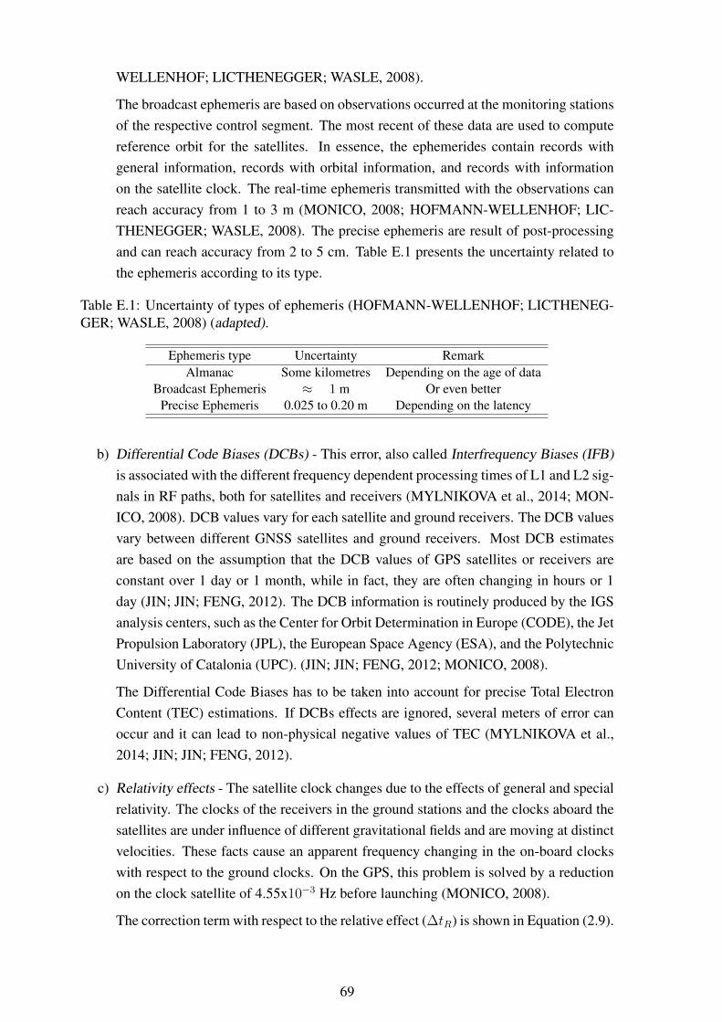
WELLENHOF; LICTHENEGGER; WASLE, 2008).

The broadcast ephemeris are based on observations occurred at the monitoring stationsof the respective control segment. The most recent of these data are used to computereference orbit for the satellites. In essence, the ephemerides contain records withgeneral information, records with orbital information, and records with informationon the satellite clock. The real-time ephemeris transmitted with the observations canreach accuracy from 1 to 3 m (MONICO, 2008; HOFMANN-WELLENHOF; LIC-THENEGGER; WASLE, 2008). The precise ephemeris are result of post-processingand can reach accuracy from 2 to 5 cm. Table E.1 presents the uncertainty related tothe ephemeris according to its type.

Table E.1: Uncertainty of types of ephemeris (HOFMANN-WELLENHOF; LICTHENEG-GER; WASLE, 2008) (adapted).

Ephemeris type Uncertainty RemarkAlmanac Some kilometres Depending on the age of data

Broadcast Ephemeris ≈ 1 m Or even betterPrecise Ephemeris 0.025 to 0.20 m Depending on the latency

b) Differential Code Biases (DCBs) - This error, also called Interfrequency Biases (IFB)is associated with the different frequency dependent processing times of L1 and L2 sig-nals in RF paths, both for satellites and receivers (MYLNIKOVA et al., 2014; MON-ICO, 2008). DCB values vary for each satellite and ground receivers. The DCB valuesvary between different GNSS satellites and ground receivers. Most DCB estimatesare based on the assumption that the DCB values of GPS satellites or receivers areconstant over 1 day or 1 month, while in fact, they are often changing in hours or 1day (JIN; JIN; FENG, 2012). The DCB information is routinely produced by the IGSanalysis centers, such as the Center for Orbit Determination in Europe (CODE), the JetPropulsion Laboratory (JPL), the European Space Agency (ESA), and the PolytechnicUniversity of Catalonia (UPC). (JIN; JIN; FENG, 2012; MONICO, 2008).

The Differential Code Biases has to be taken into account for precise Total ElectronContent (TEC) estimations. If DCBs effects are ignored, several meters of error canoccur and it can lead to non-physical negative values of TEC (MYLNIKOVA et al.,2014; JIN; JIN; FENG, 2012).

c) Relativity effects - The satellite clock changes due to the effects of general and specialrelativity. The clocks of the receivers in the ground stations and the clocks aboard thesatellites are under influence of different gravitational fields and are moving at distinctvelocities. These facts cause an apparent frequency changing in the on-board clockswith respect to the ground clocks. On the GPS, this problem is solved by a reductionon the clock satellite of 4.55x10−3 Hz before launching (MONICO, 2008).

The correction term with respect to the relative effect (∆tR) is shown in Equation (2.9).

69

In relative positioning (presented in Appendix F), the relativity effects are totality neg-ligible (MONICO, 2008).

c) Antenna Phase Center (APC) - The GNSS antenna is the connecting element betweenthe satellite and the GNSS receiver. The satellite Antenna Phase Center (APC) is thereference point for the broadcast ephemeris. This point differs from the center of massof the satellite, and it changes for different values of elevation and azimuth angles.Therefore, for high precision applications, the phase center offset vector has to betaken into account (EL-HATTAB, 2013; MONICO, 2008; DoD, USA, 1995).

The APC offset vectors, in general, are given with respect to a fixed coordinate frame,with the origin on the satellite center of mass, and shall be converted to a fixed ref-erence frame on Earth, such as ITRF2005. These values are calculated by some IGSanalysis centers (e.g. CODE and GFZ) and are provided by IGS (MONICO, 2008).

Receiver related errors

a) Interchannel errors - Nowadays, the majority of geodesic receivers present multiplechannels and in this case, a systematic interchannel error can occur, since the signalof each satellite will travel through different electronic paths. In order to correct thiseffect, the receivers have a device which calibrates and compensates these interchan-nel biases (SEEBER, 2003; MONICO, 2008). A channel is taken as the reference,each channel tracks, simultaneously, a particular satellite and determines the errorswith respect to the reference channel. This effect will be correct in all subsequentobservations.

70

Appendix F

Positioning techniques

Positioning corresponds to the determination of positions of objects with respect to aspecific reference. It can be divided into absolute positioning, when the calculated coordi-nated are directly associated with the centre of the Earth, and relative positioning, when thecoordinates are obtained with respect to an object with known coordinates. Also, the posi-tioning can be classified in static and cinematic, depending on if the object is at rest or undermovement (MONICO, 2008).

In the absolute positioning (also named Point Positioning), when the transmittedephemeris are employed, the position of the point is obtained in the reference frame of thesystem (WGS 84 for GPS, PZ90 for GLONASS). However, when precise ephemeris andclock corrections are employed, along with carrier phase data, the reference frame adoptedis related to the precise ephemeris. In addition to the classifications presented previously,the positioning can be classified as real-time and post-processed. In the first, the estimativeoccurs almost at the same time the observations are collected. In the post-processed, theestimates are obtained after the data collect (MONICO, 2008).

In the following sections the Point Positioning (PP), Precise Point Positioning (PPP) andRelative Positioning (RP) techniques will be presented.

Point Positioning

Point positioning refers to the determination of the position of a station based on pseudo-range observation, using orbit and satellite parameters broadcast in the navigation message.This positioning technique requires only a receiver and is a widely employed method forlow precision navigation. If available, it is possible to include in the processing, besides thepseudorange, the carrier phase measurements. However, this procedure is not very commonin this technique, since it does not provide an improvement in the solution for one epoch(MONICO, 2008). Therefore, this positioning technique does not satisfy the precision re-quirements for geodetic positioning.

71

The major errors that affect this positioning method are related to the quality of theobservable (pseudorange) and the accuracy of the parameters sent in the navigation message,such as ephemeris and clock. In addition, this method suffers influence of troposphericand ionospheric errors, multipath, and others. When real-time positioning is not necessary,it is possible to use precise ephemeris and satellite clock corrections, leading to a moreprecise solution. This technique is called Precise Point Positioning - PPP and will be brieflypresented in the following section (MONICO, 2008).

Precise Point Positioning

Precise Point Positioning (PPP) is a positioning method similar to the Point Positioning.However, the use of precise satellite orbits and satellite clock corrections provides a betterquality to this method (ROCHA et al., 2017; MONICO, 2008). Besides satellite orbit andclock corrections, other errors that affect the observations, such as ionospheric and tropo-spheric effects, have to be corrected in order to allow a more accurate PPP solution (ROCHAet al., 2017). The types of ephemeris provided by the IGS are presented in Appendix E.

This method presents a great potential to be used in applications that require high-accuracy, such as geodynamics, and presents great advantages when compared with theprocessing of GNSS networks, in which high-computational effort is required (MONICO,2008). Given the spread of internet use, some PPP on-line services are available to theusers (for free in some cases). These on-line services offer the positioning estimates, in thepost-processing mode, from GNSS observation sent by the users. Several on-line servicesare available, such as the Automatic Precise Positioning Service (APPS) provided by theJet Propulsion Laboratory (JPL), the MagicGNSS developed by the GMV Aerospace andDefense S.A., the Canadian Spatial Reference System (CSRS-PPP) provided by the NaturalResource Canada - NRCan. In Brazil, national initiatives such as the RT-PPP developed atthe School of Sciences and Technology of São Paulo State University (FCT/UNESP) and theIBGE-PPP provided by the Brazilian Institute of Geography and Statistics (IBGE) are alsoavailable to the users who want to perform the on-line PPP solutions (ROCHA et al., 2017).

In addition to the post-processed PPP, the real-time PPP solution has been investigatedduring the last years, achieving good accuracy results. In 2009, van Bree et al. 2009compared the results obtained in the real-time Single-Frequency PPP solution using IGSUltra-Rapid products (satellite clock error) and the REal-Time CLock Estimation (RETI-CLE) developed by at German Space Operations Center of the German Aerospace Center(GSOC/DLR) with the IGS Final clocks. The results obtained with the RETICLE satelliteclock presented an accuracy comparable with the IGS Final Products. In the work (BREE;TIBERIUS, 2012), the authors assessed the SF-PPP solution using satellite clocks and or-bits provided by RETICLE, and used GIMs and predicted DCB from the Center for OrbitDetermination (CODE). The position accuracy achieved with a kinematic approach reached

72

standard deviations of about 0.15 and 0.30 m for the horizontal and vertical coordinates,respectively, and with 95% error values of about 0.30 m and about 0.65 m, where the 95thpercentile means that 95% the error is below this amount.

The international GNSS service (IGS) has been providing an open-access real-time ser-vice (RTS) since 2013. The advent of IGS RTS products allows users to carry out real-timeprecise point positioning (RT-PPP) anywhere in the world (NIE et al., 2018). In the studycarried out by (ELSOBEIEY; AL-HARBI, 2015), the performance of RT-PPP using the IGSRTS is assessed. The accuracy obtained using the RTS products presented better accuracywhen compared to the IGS ultra-rapid products (predicted part). In addition to these studieson Real-Time PPP, a recent study carried out by (NIE et al., 2018) proposes an alternative ap-proach for GPS clock prediction in case of an outrage on RTS. These investigations in Real-Time PPP can improve applications such as high-precision agriculture, navigation applica-tions in the automotive and possibly even automated aircraft landing (BREE; TIBERIUS,2012).

Relative Positioning

The relative positioning involves the simultaneous observation of a numberm of satellitesand a minimum of two GNSS-receivers (TEUNISSEN; KLEUSBERG, 1996). However,with the advent of the Active Control Systems (ACS) it is possible to perform the relativepositioning by using only one GNSS receiver. In an ACS, the receivers perform continuoustracking of the visible satellites and the users can access the data via communication system(MONICO, 2008).

The advantage of the relative positioning is related to the fact that the parameters ofinterest are much less sensitive to interfering uncertainties such as ephemeris, clocks andatmospheric effects (TEUNISSEN; KLEUSBERG, 1996). By combining the observablesinvolved in the process of relative positioning it is possible to mitigate some systematicerrors that affect the GNSS observables errors, such as atmospheric effects and satellite clockerrors.

73