Helsinki University of Technology

Faculty of Information and Natural Sciences

Department of Mathematics and Systems Analysis

Mat-2.4108 Independent research projects in applied mathematics

Modelling Sleep Stages With

Markov Chains

13th February 2009

Väinö Jääskinen

61613T

Contents

1 Introduction 4

2 Sleep Staging 6

3 Markov Chain Model 9

4 Methods 11

5 Results 12

6 Discussion 18

References 20

LIST OF FIGURES LIST OF FIGURES

List of Figures

1 Hypnogram of a Normal night’s sleep. (Horizontal axis is 30second epochs from lights off) . . . . . . . . . . . . . . . . . . 6

2 Hypnogram of a Recovery night’s sleep. (Horizontal axis is30 second epochs from lights off) . . . . . . . . . . . . . . . . 7

3 A Simple Markov Chain . . . . . . . . . . . . . . . . . . . . . 11

5 Distribution of the mean numbers (SD) of sleep stages underNormal and Recovery conditions . . . . . . . . . . . . . . . . 15

2

LIST OF TABLES LIST OF TABLES

List of Tables

1 Time spent in different sleep stages . . . . . . . . . . . . . . . 6

2 Summary of the number of 30 second epochs under Normaland Recovery (N/R) conditions (n = 21) . . . . . . . . . . . . 14

3 Stage count differences between Normal and Recovery condi-tions . . . . . . . . . . . . . . . . . . . . . . . . . . . . . . . . . 16

4 Statistical testing of stage count differences between Normaland Recovery conditions . . . . . . . . . . . . . . . . . . . . . 17

5 Comparison of the probability matrices under the two condi-tions N(R) . . . . . . . . . . . . . . . . . . . . . . . . . . . . . 17

3

1 INTRODUCTION

1 Introduction

Sleep research is a relatively young discipline. Before the 20th century, therewere no practical methods to study sleep besides the analysis of dreams.From 1920s onwards, the invention of electroencephalography (EEG) andother advances have made it possible to better understand the electricalactivity of the brain. The discovery of rapid eye movement (REM) sleepestablished the fact that sleep is divided into phases with different charas-teristics and functions. Describing and explaining them remains a majorresearch challenge. [1]

From a clinical point of view, sleep-related pathologies are difficult to studyand cure. Long measurements in specialised laboratories are often neededfor the analysis of sleep. This can be expensive and taxing for patients andclinicians alike. Despite the difficulties, sleep medicine has advanced anddeveloped treatments to pathologies like sleep apnea and narcolepsy. Effectsof more general disturbances in sleep have also been a subject of interest.They are common and affect a significant part of the population. [1]

Sleep as a biological phenomenon is closely related with the electrical activityof the brain. Recordings of EEG, EOG (electro-oculography) and EMG(electromyography) form time series. However, recording a patient’s EEG,EOG and EMG for even a single night of sleep produces a large quantity ofdata. Therefore it is customary to classify sleep recordings into stages. Thisis possible because of the regularities in the structure of sleep. Statisticalanalysis can then be performed on the staged data. [2], [3]

Traditionally, stage scoring has been done by visually analyzing EEG, EOGand EMG recordings. This method requires an experienced sleep technicianto perform the staging. To save resources and increase accuracy, automaticstaging procedures have been developed. Among them are technical solu-tions based on, for example, pattern matching, and neural networks [4]. Atthe present moment, the traditional visual method remains the standard.Automatic procedures can be useful additional tools for visual scoring, buttheir performance as a standalone method is not satisfactory [5].

There are various ways to use the scored sleep stage data. The basic idea is torecognize structures in sleep and then link them with relevant physiologicalphenomena. For example, patients with narcolepsy usually proceed to REMsleep straight from wakefulness instead of going through other sleep stages.

4

1 INTRODUCTION

Also, correctly assessing the severity of sleep apnea benefits from sleepstaging. How then to describe the structure of sleep based on stage data?The sum of stage counts during a relevant period of time (for example, thewhole or one third of the night) is the simplest statistic used. Visual analysisis made possible by the use of hypnograms, which are graphs of sleep stagedata plotted against time. [1]

Another way to use sleep stage data is the construction of Markov models.A simple time-homogenous Markov chain was the first attempt to usethis approach [6]. Later on, semi-Markov chains [7] and time-continuousMarkov models [8] have been developed. Creating simulated hypnogramswith Monte Carlo methods is a major application for this type of models.For example, effects of aircraft noise on sleep structure can be studied.Literature reports that Markov models have been used for simulating sleepunder different conditions or scenarios. With simulated stage recordings,hypnograms and sleep parameters can be compared between conditions [9].

In this study, empirical data is analyzed for two purposes. Firstly, thefollowing hypothesis is tested: if a person has slept less than normally, theamount of Slow Wave Sleep (SWS) increases. This is a widely reportedphenomenon in the literature [10], [1]. For example, if there is a one nightwhen the subject cannot sleep normally, the next night there is probablygoing to be more SWS in her sleep. This study compares the possiblestatistical difference of the amount of SWS epochs between the Normaland Recovery nights. The hypothesis is that this approach should yield thestandard literature result of increased SWS during recovery nights.

Secondly, a Markov chain probability matrix is used to find out, how thetransitions from one stage to another are distributed. Estimating a transitionmatrix from a sample of multiple nights offers a description of the sleep’sstructure under given conditions. Furthermore, statistical comparisons ofthese matrices tell how different conditions affect the transitions betweenstages.

This study has five main parts. Section 2 describes some basic informationabout sleep stages. In Section 3 a simple Markov model is presented foranalysing sleep stage data. Also, relevant theoretical aspects are reviewed.Methods of the study are described in Section 4 and the results are presentedin Section 5. The results are discussed in Section 6 where some suggestionsfor the course of future research are made. Also, the adequacy of the usedMarkov model and other questions of validity are assessed.

5

2 SLEEP STAGING

W

SREM

S1

S2

S3

S4

0 100 200 300 400 500 600 700 800 900

Figure 1: Hypnogram of a Normal night’s sleep. (Horizontal axisis 30 second epochs from lights off)

2 Sleep Staging

Sleep can be defined theoretically as "reversible behavioral state of percep-tual disengagment from and unresponsiveness to the environment" [1]. Atthe level of common sense, we all know what sleep is, but its physiologyis an amalgam of complex phenomena. On average young people usuallysleep 7.5 hours during weeks and 8.5 hours during weekend nights. Howe-ver, this and many other aspects of sleep vary, so it is difficult to describe"normal" sleep [1].

There are three main physiological signals used for sleep staging (scoring).

Table 1: Time spent in different sleep stages

W S1 S2 S3 S4 SREM

0-5% 2-5% 45-55% 3-8% 10-15% 20-25%

6

2 SLEEP STAGING

W

SREM

S1

S2

S3

S4

0 100 200 300 400 500 600 700 800 900

Figure 2: Hypnogram of a Recovery night’s sleep. (Horizontalaxis is 30 second epochs from lights off)

7

2 SLEEP STAGING

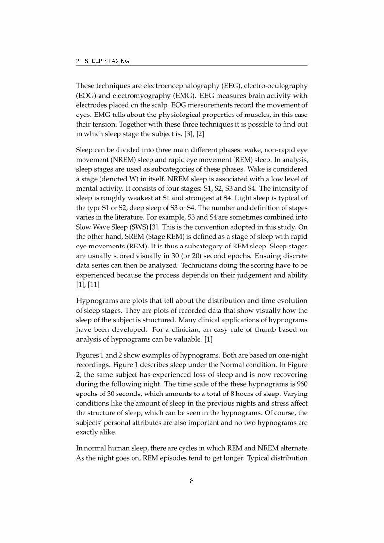
These techniques are electroencephalography (EEG), electro-oculography(EOG) and electromyography (EMG). EEG measures brain activity withelectrodes placed on the scalp. EOG measurements record the movement ofeyes. EMG tells about the physiological properties of muscles, in this casetheir tension. Together with these three techniques it is possible to find outin which sleep stage the subject is. [3], [2]

Sleep can be divided into three main different phases: wake, non-rapid eyemovement (NREM) sleep and rapid eye movement (REM) sleep. In analysis,sleep stages are used as subcategories of these phases. Wake is considereda stage (denoted W) in itself. NREM sleep is associated with a low level ofmental activity. It consists of four stages: S1, S2, S3 and S4. The intensity ofsleep is roughly weakest at S1 and strongest at S4. Light sleep is typical ofthe type S1 or S2, deep sleep of S3 or S4. The number and definition of stagesvaries in the literature. For example, S3 and S4 are sometimes combined intoSlow Wave Sleep (SWS) [3]. This is the convention adopted in this study. Onthe other hand, SREM (Stage REM) is defined as a stage of sleep with rapideye movements (REM). It is thus a subcategory of REM sleep. Sleep stagesare usually scored visually in 30 (or 20) second epochs. Ensuing discretedata series can then be analyzed. Technicians doing the scoring have to beexperienced because the process depends on their judgement and ability.[1], [11]

Hypnograms are plots that tell about the distribution and time evolutionof sleep stages. They are plots of recorded data that show visually how thesleep of the subject is structured. Many clinical applications of hypnogramshave been developed. For a clinician, an easy rule of thumb based onanalysis of hypnograms can be valuable. [1]

Figures 1 and 2 show examples of hypnograms. Both are based on one-nightrecordings. Figure 1 describes sleep under the Normal condition. In Figure2, the same subject has experienced loss of sleep and is now recoveringduring the following night. The time scale of the these hypnograms is 960epochs of 30 seconds, which amounts to a total of 8 hours of sleep. Varyingconditions like the amount of sleep in the previous nights and stress affectthe structure of sleep, which can be seen in the hypnograms. Of course, thesubjects’ personal attributes are also important and no two hypnograms areexactly alike.

In normal human sleep, there are cycles in which REM and NREM alternate.As the night goes on, REM episodes tend to get longer. Typical distribution

8

3 MARKOV CHAIN MODEL

of stages is presented in Table 1 (adapted from [1]).

3 Markov Chain Model

The idea that transitions between sleep stages can be modelled as a Markovprocess is not new. Currently, advanced models are based on continuous-time Markov chains [8], [9]. In this study we limit to a time-homogenousMarkov chain, along the lines of Zung et al.’s pioneering work [6]. Whetherthis model is detailed enough, is a serious issue. However, it has to be keptin mind that the main objective of this study is to compare stage transitionsbetween the two conditions.

This section presents basics of Markov chains and how they can be appliedto modeling sleep stages. A simple model of human sleep is developedalongside the more theoretical material. The section is based on Taylor andCarlin’s book [12].

We define a discrete time Markov chain {Xt} as a stochastic process satis-fying the following conditions:

1. The state space S is a finite or countable set.

2. The time index set is T = (0, 1, 2, . . .)

3. The chain has the Markov property, i.e. the conditional probabilitydistribution of all the possible changes in the system’s state is notaffected by knowledge of its history besides the current state.

The Markov property can be formalized as:

Pr{Xn+1 = j|X0 = i0, . . . , Xn−1 = in−1, Xn = i}= Pr{Xn+1 = j|Xn = i} (1)

for all n ∈ T and all states i0, . . . , in−1, i, j.

How does the human sleep as a process meet these criteria? We saw in the

9

3 MARKOV CHAIN MODEL

previous section that sleep can be classified into five discrete stages: W,SREM, S1, S2 and SWS. Thus it is natural to choose them as the states ofthe process, yielding S = {W, SREM, S1, S2, SWS}. As stage information isa discrete time series, there is no problem constructing the time index setT. The Markov property and time-homogenous nature of the probabilitydistribution hold at least approximately, although actual empirical datashows some non-stationary properties [6], [8], [9].

Transition probabilities of the chain {Xt} can be arranged in a n×m matrix:

P =

p11 p12 · · · p1m

p21 p22 · · · p2m...

.... . .

...pn1 pn2 · · · pnm

The probability of going from the state i to j in one step is pij.

In this study, the following transition matrix is used:

P =

pW→W pW→SREM pW→S1 pW→S2 pW→SWS

pSREM→W pSREM→SREM pSREM→S1 pSREM→S2 pSREM→SWS

pS1→W pS1→SREM pS1→S1 pS1→S2 pS1→SWS

pS2→W pS2→SREM pS2→S1 pS2→S2 pS2→SWS

pSWS→W pSWS→SREM pSWS→S1 pSWS→S2 pSWS→SWS

For example, the elements of the second row represents the probabilites oftransitions from SREM state to state x ∈ S = {W, SREM, S1, S2, SWS}. Notethat changes from a stage to itself (SREM→SREM etc.) are also consideredtransitions.

Figure 3 offers visualization of a simple Markov chain. Here, the probabilityof going from state 2 to state 3 in one step is 0.4. The total probability oftransitions from a single state is one. In the figure, impossible transitions,i.e. those having a zero probability, are not indicated. Notice that once theprocess enters state 1, it stays there indefinitely.

Next we consider the behavior of the process over multiple steps. Forexample, if the process starts at stage W, what is the probability that it willbe at SREM after 9 steps (n = 9)? We note the probability of transitionfrom state i to j in n steps with p(n)

ij . The matrix P(n) includes all transition

10

4 METHODS

1

2

4

3

0.5

0.3

0.2

0.4

0.3

0.3

0.6

0.4

Figure 3: A Simple Markov Chain

probilities for a given value of n. It can be shown (see for example [12]) thatthe n-step transition probabilites p(n)

ij are entries of nth power of the matrix

P. From this we conclude that P(n) = Pn.

The transition probability matrix P is a parameter of the Markov model. Itcan be estimated with the relative frequency of the number of transitions.For example, if there are 6 W→SREM transitions and a total number of 30transitions from W in a dataset, then pW→SREM is 0.2. By increasing thesample size, the estimation can be made more accurate because of the lawof large numbers. Note that in this study, the used datasets can be eitherrecordings of one night’s sleep or aggregates over multiple nights. Whenit comes to estimating the probability matrices, this does not change theprocedure.

4 Methods

In the dataset, there are 21 normal male adult subjects with an age range of18-22 (mean 21). The study design has been reported earlier by Sallinen et al.

11

5 RESULTS

[13]. The subjects’ sleep was studied during five nights. The first night wasto screen for sleep disorders which would have disqualified subjects fromthe study. Two nights were normal nights. The latter of those was used here.Then, a night with only two hours for was sleeping followed by a Recoverynight.

In this study, the nights used form the data mentioned above are the Normalnight and the Recovery night. The equipment used was digital Embla N7000(EMBLA, Broomfield, CO, USA). One experienced sleep technician scoredthe recordings visually. The standards used were normal EEG, EOG, andEMG montage [3].

A wide concensus exists in the literature that there should be more SlowWave Sleep (SWS) under Recovery conditions [13]. This study has tworesearch questions. Firstly, can the SWS-hypothesis be verified by comparingthe epoch counts under the two conditions? For this, the data is categorizedby subject and a paired Wilcoxon test is performed to see the differencesbetween the Normal and Recovery conditions. The second question is, howdo the same conditions affect the transitions? There is no clear hypothesisavailable so this part of the study is explorative in nature. The change ofstages over time is modelled as a Markov chain. Transition probabilitesare estimated by calculating the relative frequencies of transitions with acustomized Delphi-based software crated by the author. A paired Wilcoxontest is then conducted on the estimated transition matrices. The reportedp-values are uncorrected. Statistical tests are performed with R [14].

5 Results

The first result of the data analysis is the distribution of epochs categorizedby subject and condition. Note that the count of epochs for any stage isequivalent to the number of transitions from (or to) that stage. After eachepoch spent in a stage there occurs a transition. This follows from the logicof the Markov chain model presented in the Section 3.

Graphs of the stage count data (Figure 4) show that the conditions seem tohave a systematic effect on the stage counts. The variation between subjectswas most emphasised in the W stage (Figure 4a).

Table 2 presents a summary of the epoch count data under the two conditions.

12

5 RESULTS

W Epochs

0

20

40

60

80

100

120

140

1 2 3 4 5 6 7 8 9 10 11 12 13 14 15 16 17 18 19 20 21

NR

(a)

SREM Epochs

0

50

100

150

200

250

300

350

1 2 3 4 5 6 7 8 9 10 11 12 13 14 15 16 17 18 19 20 21

NR

(b)

S1 Epochs

0

20

40

60

80

100

120

1 2 3 4 5 6 7 8 9 10 11 12 13 14 15 16 17 18 19 20 21

NR

(c)

S2 Epochs

0

100

200

300

400

500

600

700

1 2 3 4 5 6 7 8 9 10 11 12 13 14 15 16 17 18 19 20 21

NR

(d)

SWS Epochs

0

50

100

150

200

250

300

350

400

1 2 3 4 5 6 7 8 9 10 11 12 13 14 15 16 17 18 19 20 21

NR

(e)

Figure 4: Distribution of epochs categorized by subject and condi-tion

Both Normal and Recovery conditions are listed. For example, the standarddeviation of the number of S2 epochs was 69 (Normal) and 72 (Recovery).The variation between data points was probably caused by subjects’ personaltraits, the effect of conditions, and measurement errors.

13

5 RESULTS

Table 2: Summary of the number of 30 second epochs under Nor-mal and Recovery (N/R) conditions (n = 21)

W (N/R) SREM (N/R) S1 (N/R) S2 (N/R) SWS (N/R)

Mean 58/35 218/206 61/45 449/468 217/272SD 32/24 62/64 22/15 69/72 56/58Median 52/26 209/229 61/48 439/460 226/278Min 12/7 104/98 12/13 326/364 121/123Max 123/87 318/318 102/79 608/619 330/373

For testing the SWS-hypothesis, Figure 4e offers essential information. Vi-sual comparison of the stage counts suggests there was more SWS duringRecovery nights than Normal nights. This confirms the SWS-hypothesis, atleast based on this data.

Figure 5 presents the means and the standard deviation (SD) of epoch counts.The most common stage is S2, which we can also see from Figure 4. Again,there was a difference in SWS between Normal and Recovery conditions.This difference seems to be proportionally clearest among the stages.

After visually examining the distributions of stage counts, we proceed toresults of statistical testing. The SWS-hypothesis is tested by pairwise com-parison of stage count data. These results were then compared with thetransition probabilites of the Markov matrix. Besides this, statistical depen-dencies between stage transitions (not only SWS) were investigated.

Table 3 includes the differences of stage counts under the two conditions.The value of the Normal night is substracted from that of the Recovery night.Note that here the percentage values are differences of relative frequencies,not percentage changes between the two conditions. For example, subject2 had a difference of -9 in SREM stage between Normal and Recoveryconditions. The reported percentage value 1% was the difference of therelative frequencies (26.5% for Normal and 27.6% for Recovery) of the SREMstage. The relative or absolute frequencies are not reported in the table, onlytheir differences. Likewise, the percentage change for subject 2 in SREMwould be 11% as it increases from 263 (Normal) to 292 (Recovery).

The results of the Wilcoxon Rank test (confidence interval 95%) are reportedin Table 4. The test showed that there were statistically significant differences

14

5 RESULTS

0

100

200

300

400

500

600

W SREM S1 S2 SWS

NormalRecovery

Figure 5: Distribution of the mean numbers (SD) of sleep stagesunder Normal and Recovery conditions

15

5 RESULTS

Table 3: Stage count differences between Normal and Recoveryconditions

Subject W SREM S1 S2 SWS

1 -6 (-1%) -6 (6%) -38 (-4%) 9 (-1%) 5 (0%)2 -9 (-1%) -9 (1%) -46 (-5%) 63 (4%) 29 (1%)3 -12 (-1%) -12 (-11%) -20 (-2%) 101 (8%) 67 (6%)4 14 (1%) 14 (0%) 7 (0%) -26 (-6%) 63 (5%)5 -15 (-2%) -15 (-4%) -48 (-5%) 70 (4%) 83 (7%)8 -68 (-7%) -68 (0%) -11 (-2%) 40 (0%) 101 (8%)9 -37 (-3%) -37 (-4%) -25 (-2%) -16 (3%) 47 (7%)

10 13 (1%) 13 (-8%) 34 (3%) 60 (1%) 69 (4%)11 -27 (-3%) -27 (-4%) -5 (-1%) -24 (-5%) 143 (12%)12 -67 (-6%) -67 (2%) -35 (-3%) -11 (-1%) 100 (9%)13 -3 (-1%) -3 (-2%) 3 (0%) -42 (-7%) 96 (9%)14 6 (1%) 6 (-8%) -41 (-4%) 134 (13%) -18 (-2%)15 -108 (-11%) -108 (7%) -22 (-2%) 4 (-1%) 74 (6%)16 -2 (0%) -2 (-2%) -53 (-5%) 43 (4%) 40 (4%)17 -4 (0%) -4 (2%) -17 (-2%) -62 (-7%) 83 (8%)18 15 (1%) 15 (4%) -8 (-1%) -79 (-10%) 74 (6%)19 -24 (-2%) -24 (-2%) 20 (2%) -24 (-2%) 42 (4%)20 -76 (-8%) -76 (3%) 3 (0%) 71 (4%) 29 (1%)21 -8 (-1%) -8 (-7%) 1 (0%) 32 (5%) 17 (3%)

Mean -23,5 (-2%) -11,6 (-2%) -15,4 (-2%) 19,38 (1%) 55 (5%)SD 33,87 (3%) 52,45 (5%) 23,07 (2%) 58,06 (6%) 40,17 (4%)

Median -12 (-1%) -7 (-2%) -17 (-2%) 9 (1%) 63 (5%)Min -108 (-11%) -104 (-11%) -53 (-5%) -79 (-10%) -18 (-2%)Max 15 (1%) 86 (7%) 34 (3%) 134 (13%) 143 (12%)

16

5 RESULTS

Table 4: Statistical testing of stage count differences between Nor-mal and Recovery conditions

Test Statistic p-value

W ?? 28 0.001SREM 72 0.137

S1 ?? 37 0.005S2 133 0.562

SWS ??? 223 < 0.001

Wilcoxon Signed Rank test for paired data, ? equals p < 0.05, ?? p < 0.01, and ??? p < 0.001

Table 5: Comparison of the probability matrices under the twoconditions N(R)

W SREM S1 S2 SWSW 66%(49%)??? 2%(4%) 23%(28%) 9%(18%)? 0%(2%)

SREM 2%(2%) 95%(95%) 2%(2%) 1%(2%)?? 0%(0%)S1 7%(6%) 4%(4%) 49%(48%) 40%(41%) 0%(0%)S2 2%(2%) 1%(2%) 3%(2%)? 88%(88%) 5%(6%)

SWS 1%(1%) 0%(0%) 0%(0%) 10%(10%) 89%(89%)

Wilcoxon Signed Rank test for paired data , ? equals p < 0.05, ?? p < 0.01, and ??? p < 0.001

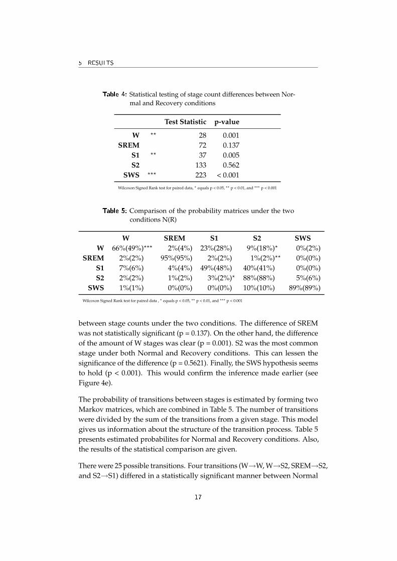
between stage counts under the two conditions. The difference of SREMwas not statistically significant (p = 0.137). On the other hand, the differenceof the amount of W stages was clear (p = 0.001). S2 was the most commonstage under both Normal and Recovery conditions. This can lessen thesignificance of the difference (p = 0.5621). Finally, the SWS hypothesis seemsto hold (p < 0.001). This would confirm the inference made earlier (seeFigure 4e).

The probability of transitions between stages is estimated by forming twoMarkov matrices, which are combined in Table 5. The number of transitionswere divided by the sum of the transitions from a given stage. This modelgives us information about the structure of the transition process. Table 5presents estimated probabilites for Normal and Recovery conditions. Also,the results of the statistical comparison are given.

There were 25 possible transitions. Four transitions (W→W, W→S2, SREM→S2,and S2→S1) differed in a statistically significant manner between Normal

17

6 DISCUSSION

and Recovery conditions. In W→W and S2→S1, the probability was greaterunder the Normal condition. This also held for SWS→S1, but the differencewas not statistically significant. In all the other 22 transitions, the proba-bility was greater under Recovery conditions. The difference was greatestin W→W transitions (66% for N and 49% for R). This was balanced by adecrease in the probability of W→S2 transitions (9% for N and 18% for R).The changes between conditions in the W-row matrix (transitions from W)were more numerous than in other rows.

Earlier in this section, the SWS-hypothesis was analyzed. The differencebetween conditions in the amount of epochs was greatest in the SWS stage.This held for both the absolute proportional change (see Table 3). Now theinteresting question is, how does this affect probabilites of SWS transitions?Surprisingly, Table 5 shows that the SWS row (transitions from SWS) wasunaffected. Thus the increase of SWS under Recovery conditions did notseem to lead to any clear changes in the probabilites of transitions from andto the the SWS stage. Futher analysis could focus on the interaction of Wand SWS stages as they seem to react differences of conditions more activelythan other stages.

6 Discussion

In this study, the structure of sleep was studied under two conditions, Nor-mal and Recovery. The first method was the comparison of epoch counts.The second was using a Markov chain model to describe the probability oftransitions between sleep stages. Both were applications of existing theories.

Firstly, the comparison of epoch counts showed that there were more SWSepochs under the Recovery conditions than Normal conditions. This confir-med the SWS-hypothesis. It seems then natural to conjure that there wouldbe more SWS→SWS transitions under the Recovery conditions. However,this was not the case. The Markovian approach showed that the statisti-cally significant transition differences were in W→W and W→S2, W→SWS,SREM→S2, and S2→S1. Under the Recovery conditions there were fewerW epochs, i.e. the subject has slept more. Two out of the four differencesoccured in transitions from the W stage. Thus the interaction of W with otherstages was more evident than that of SWS. This calls for futher investigation.

The different behavior of the epoch count and transition probabilites of SWS

18

6 DISCUSSION

are examples of new knowledge that can be obtained by using a Markovchain approach. However, the model used here is relatively simple whencompared with continuous-time Markov models reported in the literature.Introducing a unique matrix for each epoch as opposed to just one for thewhole night would be a major change. Also, other more powerful propertiesof the Markovian theory could be used. For example, the question of whenthe SWS stage is first reached is interesting. However, in order to benefitfrom these measures, research questions and perhaps also the study designwould need changes. The clearest differences between conditions can beperhaps detected with a simple model, like the one used here. Creatingsimulated hypnograms with this model is not very meaningful, becausethey would not provide new information about the process. The situationis different with a multiple-matrix, i.e. a continous-time model, where theproperties of the process cannot be calculated directly from the transitionprobability matrices.

One limitation of this study is that there are only two conditions (Normaland Recovery). A possible way to expand the area of study is to increasethe number of testing conditions. Sleep disorders, sex, age etc. could be va-luable conditions for assessing the structure of sleep. This would give moreinformation about the sleep structure under different conditions. Futher-more, the reasonability of the whole Markovian approach could be assessed.If the Markov model suggests new ideas that can be tested empirically, itcontributes to the development of sleep science. Clinical work is a primeexample. By supplementing traditional hypnograms, Markov matrices canperhaps help to diagnose pathologies by providing more detailed informa-tion about transitions between sleep stages. However, it takes time for thesleep medicine community to accept new practices. Results should be morethoroughly intrepreted in the light of current sleep research theories, a taskbeyond the scope of this special study [15].

19

REFERENCES REFERENCES

References

[1] M.H. Kryger, T. Roth, and W.C. Dement. Principles and practice of sleepmedicine. Saunders Philadelphia, 2000.

[2] C. Iber, S. Ancoli-Israel, A. Chesson, and SF Quan. for the AmericanAcademy of Sleep Medicine. The AASM manual for the scoring of sleep andassociated events: rules, terminology and technical specifications. Westchester,IL: American Academy of Sleep Medicine, 2007.

[3] A. Rechtschaffen, A. Kales, et al. A Manual of Standardized Terminology,Techniques and Scoring System for Sleep Stages of Human Subjects. BrainInformation Service/Brain Research Institute UCLA, Los Angeles, 1968.

[4] P. Anderer, G. Gruber, S. Parapatics, M. Woertz, T. Miazhynskaia,G. Klosch, B. Saletu, J. Zeitlhofer, MJ Barbanoj, H. Danker-Hopfe, et al.An E-health solution for automatic sleep classification according toRechtschaffen and Kales: validation study of the Somnolyzer 24 x 7utilizing the Siesta database. Neuropsychobiology, 51(3):115–33, 2005.

[5] V. Svetnik, J. Ma, K.A. Soper, S. Doran, J.J. Renger, S. Deacon, andK.S. Koblan. Evaluation of automated and semi-automated scoring ofpolysomnographic recordings from a clinical trial using zolpidem inthe treatment of insomnia. Sleep, 30(11):1562–74, 2007.

[6] W.W. Zung, T.H. Naylor, D.T. Gianturco, and W.P. Wilson. Computersimulation of sleep EEG patterns with a Markov chain model. RecentAdv Biol Psychiatry, 8:335–55, 1965.

[7] M.C. Yang and C.J. Hursch. The use of a semi-Markov model fordescribing sleep patterns. Biometrics, 29(4):667–76, 1973.

[8] B. Kemp and H.A. Kamphuisen. Simulation of human hypnogramsusing a Markov chain model. Sleep, 9(3):405–14, 1986.

[9] M. Basner. Markov state transition models for the prediction of changesin sleep structure induced by aircraft noise (Forschungsbericht 2006-07),2006.

[10] R.J. Berger and I. Oswald. Effects of Sleep Deprivation on Behaviour,Subsequent Sleep, and Dreaming. The British Journal of Psychiatry, 108(455):457, 1962.

[11] B. Richard. Sleep medicine pearls. Hanley & Belfus, 2003.

20

REFERENCES REFERENCES

[12] H.M. Taylor and S. Karlin. An introduction to stochastic modeling. Aca-demic Press.

[13] M. Sallinen, A. Holm, J. Hiltunen, K. Hirvonen, M. Härmä, J. Koskelo,M. Letonsaari, R. Luukkonen, J. Virkkala, and K. Müller. Recovery ofCognitive Performance from Sleep Debt: Do a Short Rest Pause and aSingle Recovery Night Help? Chronobiology International, 25(2):279–296,2008.

[14] R.D.C. Team. R: A language and environment for statistical computing.Vienna, Austria: R Foundation for Statistical Computing, 2004.

[15] C. Cirelli and G. Tononi. Is sleep essential. PLoS Biol, 6(8):e216, 2008.

21