modelling the australian dollar - reserve bank of · modelling the australian dollar jonathan...

Research Discussion Paper

Modelling the Australian Dollar

Jonathan Hambur, Lynne Cockerell, Christopher Potter, Penelope Smith and Michelle Wright

RDP 2015-12

The contents of this publication shall not be reproduced, sold or distributed without the prior consent of the Reserve Bank of Australia and, where applicable, the prior consent of the external source concerned. Requests for consent should be sent to the Head of Information Department at the email address shown above.

ISSN 1448-5109 (Online)

The Discussion Paper series is intended to make the results of the current economic research within the Reserve Bank available to other economists. Its aim is to present preliminary results of research so as to encourage discussion and comment. Views expressed in this paper are those of the authors and not necessarily those of the Reserve Bank. Use of any results from this paper should clearly attribute the work to the authors and not to the Reserve Bank of Australia.

Enquiries:

Phone: +61 2 9551 9830 Facsimile: +61 2 9551 8033 Email: [email protected] Website: http://www.rba.gov.au



Research Discussion Paper 2015-12

October 2015

International Department Reserve Bank of Australia

The authors would like to thank Adam Cagliarini, Marion Kohler, Daniel Rees, Chris Ryan and Mark Wyrzykowski for helpful comments and suggestions, and Chamath De Silva and Florian Weltewitz for earlier work on this topic. The views expressed in this paper are those of the authors and do not necessarily reflect the views of the Reserve Bank of Australia. The authors are solely responsible for any errors.

Authors: cockerelll, potterc, smithp and wrightm at domain rba.gov.au

Media Office: [email protected]

i

Abstract

This paper outlines an error correction model (ECM) of the Australian dollar real trade-weighted index (RTWI), which is one of the approaches used by Reserve Bank staff as a starting point for thinking about the level of the exchange rate. This particular model is designed to help answer a specific question, namely: What is the level of the exchange rate that would be expected to prevail over the medium term based on the exchange rate’s historical relationships with other theoretically and empirically relevant variables?

Notwithstanding the well-documented difficulties in empirically modelling exchange rates, the ECM has displayed robust explanatory power for a number of decades, in large part due to the strong historical relationship between Australia’s terms of trade and the real exchange rate. That said, it is still worth considering whether two recent unusual economic forces – namely, Australia’s resources boom and the adoption of unconventional monetary policy by several major foreign central banks – have been adequately captured by the model.

With this purpose in mind, the paper also discusses several extensions to the ECM. Overall, these extensions provide little evidence that the relationships between the RTWI and its historical determinants have changed substantially over time. While there is some evidence that unusual economic forces did contribute to the exchange rate being somewhat higher in recent years than would otherwise have been the case, we do not find compelling evidence of omitted variables that have substantially influenced the exchange rate over a longer period of time.

JEL Classification Numbers: C32, F31, F41 Keywords: Australian dollar, error correction model, exchange rates, resources

boom, unconventional monetary policy

ii

Table of Contents

1. Introduction 1

2. Literature Review 3

3. The Baseline ECM 7 3.1 The Terms of Trade 9 3.2 The Real Interest Rate Differential 12 3.3 Model Estimates 13 3.4 A Rolling Error Correction Model 17

4. A Markov-switching Model 19

5. Incorporating Australia’s Resources Boom 23 5.1 The Bulk Commodity Sector’s Interaction with the Rest of the Economy 24

5.1.1 The effect of bulks prices on the rest of the economy 25 5.1.2 Is investment a better indicator of the effect of higher bulks prices? 30

5.2 Bulk Commodity Prices and Expectations 36 5.2.1 Is the exchange rate more responsive to a forward-looking terms of trade? 38

6. Incorporating Unconventional Monetary Policy 41 6.1 Policy Rates and Longer-term Rates 44 6.2 Long- and Short-term Real Interest Rate Differentials 45

7. Conclusion 49

Appendix A: Out-of-sample Forecasting 51

Appendix B: Markov-switching Model Output 57

References 58



1. Introduction

The decision to float the Australian dollar in 1983 is widely recognised as having been beneficial for the Australian economy (Beaumont and Cui 2007; Stevens 2013). In particular, the floating exchange rate has played a crucial role in buffering the Australian economy from external shocks, in part by allowing the Reserve Bank of Australia (RBA) to better control domestic monetary conditions.

Although the exchange rate has been market-determined for many years, interest in assessing its level relative to some ‘benchmark’ remains strong. This interest has resulted in a broad range of theoretical and statistical models being developed to examine this, both in the academic literature and by practitioners. In part, this variation reflects well-documented difficulties in explaining the behaviour of exchange rates. More fundamentally though, it reflects differences in the questions being addressed: for example, a model that seeks to test theories about the determinants of exchange rates will differ from a model that seeks to forecast future levels of the exchange rate or to estimate the level of the exchange rate that is likely to help achieve particular economic outcomes.

This paper focuses on the level of the real exchange rate. More specifically, it attempts to quantify the extent to which the real exchange rate is consistent with the level that would be expected based on its historical relationship with other variables. While this approach will not directly answer the question of whether a given level of the real exchange rate is likely to help achieve particular economic outcomes, it may nevertheless provide a useful starting point for such discussions.1

Against this background, this paper describes an error correction model (ECM) of the Australian dollar real trade-weighted index (RTWI). The ECM estimates an ‘equilibrium’ level of the exchange rate based on its historical relationships with

1 For a discussion of some of the difficulties in using formal models to assess the level of the

exchange rate that is likely to help achieve particular economic outcomes, see Stevens (2013).

2

variables that are likely to have affected the RTWI over the medium term (and which also have a theoretical justification for doing so). Quantifying the extent to which the RTWI is consistent with the ECM’s ‘equilibrium’ level is one of the methods used by RBA staff as a starting point when thinking about the level of the exchange rate, and so complements, but is not a substitute for, a broader analysis of economic indicators and other models that have been developed by RBA staff.2

Despite the well-documented difficulties in empirically explaining movements in exchange rates, the RTWI has displayed a strong and consistent relationship with the model’s key explanatory variables – most notably the terms of trade – over the medium term. Nevertheless, the RTWI has on occasion displayed large and/or persistent divergences from the model-implied ‘equilibrium’. While such divergences are typically explained largely by the model’s short-run dynamics, it is nevertheless still worth examining whether they also reflect other factors that are not adequately captured in the baseline model.

In view of this, this paper examines the deviation between the observed RTWI and the ECM’s estimated equilibrium RTWI in recent years in more detail, and considers whether there is evidence that ‘unusual’ factors held up the value of the Australian dollar during this period. This is done in two ways. First, the baseline model is used to examine whether there is any evidence that the estimated relationships between the RTWI and the standard explanatory variables have changed over time. Second, the baseline model is augmented with additional explanatory variables in an attempt to capture two of these potential ‘unusual’ influences more directly: the resources boom; and foreign central banks’ use of unconventional monetary policies. The intent of this latter exercise is to examine whether these recent developments have revealed some omitted variables that have always been theoretically and empirically relevant determinants of the RTWI, but which have previously been more difficult to identify.

2 Other models developed by RBA staff which can help to answer a range of broader questions

about the relationships between the exchange rate and other macroeconomic variables include: the DSGE model set out in Rees, Smith and Hall (2015), which models the exchange rate using the uncovered interest parity relationship; the Bayesian vector autoregression model set out in Langcake and Robinson (2013); and the structural vector autoregression model set out in Manalo, Perera and Rees (2014).

3

The remainder of this paper proceeds as follows. The next section provides a high-level review of the theoretical and empirical exchange rate literatures. Section 3 then provides an overview of the baseline model, while Section 4 examines whether there is any evidence that the relationships between the RTWI and the baseline model’s explanatory variables have changed systematically over time using a Markov-switching extension. Sections 5 and 6 then motivate and present augmented versions of the baseline model that attempt to better incorporate Australia’s resources boom and foreign central banks’ unconventional monetary policy actions through the addition of different explanatory variables. Section 7 concludes.

All of the analysis in this paper uses data available up until the end of 2014. To preview the results, the paper does find some evidence that ‘unusual’ influences have had some effect on the RTWI in recent years, although it is difficult to quantify these effects. Overall, despite these unusual influences, the baseline ECM continues to display robust explanatory power and none of the extensions presented in this paper is clearly superior over a relatively long time period.

2. Literature Review

The theoretical and empirical literature on modelling exchange rates is large and varied. In broad terms, the literature attempts to determine the ‘equilibrium’ level of the exchange rate using a set of ‘fundamental determinants’, with this choice of determinants usually being guided by a theoretical framework. However, the determinants, the theoretical frameworks and the concepts of ‘equilibrium’ vary significantly. Moreover, even for the same set of determinants, the mechanisms through which these determinants are expected to affect exchange rates can differ. For example, a given determinant could affect the real exchange rate by influencing the nominal exchange rate, the relative price level, or a combination of the two.

This review will focus on the strand of literature that uses macroeconomic models of exchange rates, as the baseline ECM – which is set out below in Section 3 – fits within this category.3 These types of models typically attempt to explain relatively

3 For a more detailed taxonomy of the different types of macroeconomic exchange rate models,

see Driver and Westaway (2004).

4

low frequency movements in exchange rates. However, it is first worth noting that there are a range of alternative approaches to exchange rate modelling that are beyond the scope of this paper, but which may, for example, be better-suited to explaining higher-frequency exchange rate movements. A number of these alternative approaches relax the implicit assumption in macroeconomic models that foreign exchange markets are efficient and are comprised of homogenous participants with rational expectations.4

The broad category of macroeconomic models encompasses a number of different approaches. Three of the most prevalent are purchasing power parity (PPP), macroeconomic balance models, and what Clark and MacDonald (1999) term ‘behavioural equilibrium exchange rate’ models.

Perhaps the most basic concept of an ‘equilibrium’ exchange rate is based on the theory of PPP. The PPP concept is a generalisation of the law of one price, which states that, under certain conditions, the price of any particular tradeable good or service should be the same in all countries when expressed in terms of a common currency. As the law of one price should hold for all tradeable goods and services, currency-adjusted price levels in all countries should be the same, and so ‘equilibrium’ real exchange rates should be constant. Given this, empirical examinations of PPP are often carried out by testing whether real exchange rates revert to a constant mean. The results from this literature are mixed, but in general indicate that where PPP is found to hold, real exchange rates revert to their means at best quite slowly (Rogoff 1996; Taylor and Taylor 2004).

One reason for these mixed results is that real exchange rates are typically measured by deflating the nominal exchange rate using a broad measure of relative price levels, such as one based on consumer price indices. This PPP approach is conceptually appealing as it measures the real exchange rate as the price of a broadly representative basket of goods and services in one country relative to

4 For example, the microstructure approach relaxes the assumption of perfect information. It

models the exchange rate as a function of the order flow, which is assumed to reflect private information that is subsequently disseminated into the market (e.g. Evans and Lyons 2002). In contrast, the heterogeneous agent approach introduces agents with differing beliefs (e.g. De Grauwe and Grimaldi 2006). Other strands of the literature assume that markets are incomplete, and allow factors such as financial flows and changes in financial intermediaries’ risk-bearing capacity to influence exchange rates (e.g. Gabaix and Maggiori 2015).

5

another country (or a number of other countries), expressed in a common currency. However, it will include both tradeable and non-tradeable components, and there is no reason to expect PPP to hold for the latter.

In particular, Balassa (1964) and Samuelson (1964) postulated that prices for non-tradeable items – and therefore any real exchange rate that is constructed using a basket that includes those items – should be higher in countries that have relatively high productivity in their tradeable sectors. The intuition is that higher productivity in the tradeable sector will lead to higher wages in the whole economy and hence to higher prices in the non-tradeable sector. Therefore, the overall price level in this economy, and the (broadly measured) real exchange rate, will be higher, relative to that of another economy with lower productivity in its tradeable sector.

As differential trends in productivity can last for extended periods, the Balassa-Samuelson effect can help to explain why real exchange rates do not appear to revert back to a constant mean (or at least only do so very slowly). Nevertheless, both the basic and Balassa-Samuelson augmented notions of PPP are very long term concepts that do little to help explain short- or medium-term movements in exchange rates, particularly in an empirical sense. To this end, large parts of the theoretical and empirical exchange rate literature are focused on identifying short- or medium-term factors that can affect exchange rates.

One such approach is to use a macroeconomic balance (MB) model, which was first popularised by Williamson (1985). These models are also sometimes referred to as fundamental equilibrium exchange rate models.5 In these models, the equilibrium real exchange rate is defined as the level that is consistent both with internal and external balance; that is, with output at its potential level and the underlying current account balance at its ‘sustainable’ level. However, as both potential output and a sustainable underlying current account balance are difficult to quantify objectively, the estimation and interpretation of MB models requires a relatively large degree of judgement. For example, some of these models simply make ad hoc assumptions about the sustainable level of the underlying current account balance. Alternatively, in cases where the sustainable current account is modelled more formally, these models still require an assessment of ‘equilibrium’

5 Dvornak, Kohler and Menzies (2003) present a MB model of the Australian dollar.

6

or ‘desired’ policy settings (Clark and MacDonald 1999; Driver and Westaway 2004).6

Another approach is to use models that attempt to explain the exchange rate based on the observed values of relevant economic variables. These models are sometimes referred to as behavioural equilibrium exchange rate (BEER) models and, consistent with their use of explanatory variables that are measured based on observed rather than sustainable levels, they tend to have a shorter-term focus than MB models (Clark and MacDonald 1999). The types of explanatory variables included in these models vary depending on the underlying theoretical framework used. Examples include: monetary models, which focus on monetary shocks to the nominal exchange rate and so include variables such as nominal interest rates, the money supply or inflation, and GDP or income; and external balance models, which focus on the determinants of the current account balance and so include variables such as the terms of trade, interest rates, the net foreign asset position and the level of government debt or fiscal deficits.7 Given the forward-looking nature of foreign exchange markets, such models often incorporate expectations for these variables (e.g. Chen, Rogoff and Rossi 2010).

While BEER models of major floating exchange rates have often been shown to perform reasonably well within sample, they perform less well out of sample. Meese and Rogoff (1983) document this for monetary models, while subsequent papers have tended to confirm this finding for other types of BEER models (Cheung, Chinn and Pascual (2005), amongst others). Nevertheless, one set of currencies that generally offer an exception to the Meese and Rogoff (1983) finding are so-called ‘commodity currencies’, such as the Australian dollar (Gruen and Kortian 1996) and the Canadian dollar (Amano and van Norden 1995). The better out-of-sample fit is likely to reflect the fact that there is a fairly consistent role for commodity prices in explaining movements in these currencies. For example, using time series analysis both Chen and Rogoff (2003) and Cashin,

6 The IMF’s External Balance Assessment model is a prominent example of this approach. For

information on this model, see IMF (2013). 7 In the literature, monetary models are often considered to be separate from BEER models.

However, we group them together for ease of exposition, given that both attempt to explain fluctuations in the exchange rate using observed values of relevant economic variables. Notable early examples of monetary models include the Frenkel (1976) flexible price model and the Dornbusch (1976) sticky price ‘overshooting’ model.

7

Céspedes and Sahay (2004) find evidence that commodity prices influence the exchange rates of a number of commodity-exporting economies. Cayen et al (2010) reach a similar conclusion using a panel model with a latent factor that is correlated with commodity prices.

Consistent with this, previous RBA papers that have presented models of the Australian dollar have found a significant role for the terms of trade (ToT) – which is driven largely by commodity prices – in explaining the exchange rate (e.g. Gruen and Wilkinson 1991; Blundell-Wignall, Fahrer and Heath 1993; Tarditi 1996; Beechey et al 2000; Stone, Wheatley and Wilkinson 2005).

3. The Baseline ECM

The baseline ECM is specified to address the following question:

What is the level of the exchange rate that would be expected to prevail over the medium term based on the exchange rate’s historical relationships with other theoretically and empirically relevant variables?

Consistent with the literature’s approach to modelling commodity currencies, this model is best described as a BEER model. BEER models are particularly suited to answering the above question as they model the exchange rate as a function of the observed values of relevant economic variables. Nevertheless, it is important to reiterate that this type of model does not attempt to directly estimate the level of the exchange rate that is consistent with desired economic outcomes.

The baseline model is similar to the specification used in Stone et al (2005), which, in turn, was based on Beechey et al (2000).8 The model is an error correction model (ECM) of the RTWI, which estimates an equilibrium relationship between the (log) RTWI, the (log) goods ToT, and a real interest rate differential (RIRD) which is measured as the real policy rate differential between Australia and G3 economies:

8 Nevertheless, there are a few small differences. Most notably, the dummy variable – which

was included in the Stone et al (2005) model to account for a sustained period of divergence between the RTWI and the ToT in the late 1990s and early 2000s – is no longer included.

8

( )1 1 1 2 1 .t t t t tRTWI RTWI ToT RIRD SRvariablesµ γ β β ε− − −Δ = + + + + + (1)

The estimated equilibrium RTWI is the level that the model indicates is consistent with the level of the medium-term determinants (i.e. the ToT and the RIRD) and which should, based on relationships observed in the sample period, exert itself over time. The rate at which the RTWI is expected to converge to this equilibrium is indicated by the speed-of-adjustment coefficient, γ (also known as the error correction coefficient).

The estimation uses a single equation, rather than a system of equations for each of the cointegrating variables. While this can lead to a loss of efficiency in estimation and make it difficult to interpret the estimated cointegrating relationship, Johansen (1992) suggests the single equation approach is equivalent to the system of equations approach as long as there is only one cointegrating relationship between the variables and all other variables are weakly exogenous with respect to the parameters of the cointegrating relationship (in the sense of Engle, Hendry and Richard (1983)). Robustness tests suggest that both of these conditions are likely to hold in the context of this particular model, as well as for the various extensions presented later.9

As the variables in the cointegrating relationship are the determinants of the model-implied ‘equilibrium’ RTWI, it is important that their inclusion can be justified on theoretical and empirical grounds. A model that fits the data well, but makes no theoretical sense, is of limited usefulness for policy purposes as it provides no insight into the drivers of the exchange rate. The same can be said of a model that is theoretically justified, but does not perform well empirically. Discussions of the justifications for including the ToT and the RIRD follow in Sections 3.1 and 3.2. 9 Johansen tests of cointegration suggest that there is only one cointegrating relationship for the

baseline model and the extensions presented in this paper. Regarding weak exogeneity, a number of papers have noted that the ToT may not be weakly exogenous with respect to the RTWI, reflecting gradual nominal price adjustments and incomplete pass through of exchange rate movements (e.g. Chen and Rogoff 2003). Stone et al (2005) note that these issues are more likely to be evident in services trade and so use the goods ToT, in place of the goods and services ToT, in modelling the Australian dollar. We follow their methodology. Formal tests performed using a vector error correction model approach also suggest that the cointegrating variables (other than the RTWI) are weakly exogenous. Again this is true for both the baseline model and the other models that are subsequently presented in this paper.

9

The model also includes a number of additional variables (denoted SRvariables in Equation (1)), which are incorporated to account for shorter-term influences on the exchange rate. Specifically, the cointegrating variables are also included as changes (as opposed to just levels) in order to account for dynamic effects and potential serial correlation. Additional short-run variables also include the CRB index (a widely followed market-based commodity price measure) and two variables that are intended to capture ‘risk sentiment’ in financial markets: the (real) US S&P 500 equity index and the VIX (an index of option-implied expectations of volatility in the S&P 500). All of the short-run variables enter in first differences:

( )1 1 1 2 1 1 2 1

3 4 5 1 6 7 .t t t t t t

t t t t t t

RTWI RTWI ToT RIRD CRB CRBSPX VIX RTWI ToT RIRD

µ γ β β α αα α α α α ε

− − − −

−

Δ = + + + + Δ + Δ+ Δ + Δ + Δ + Δ + Δ +

(2)

The model is focused on explaining movements in the exchange rate over the medium term. Reflecting this focus, the model is estimated at a quarterly (rather than, say, a daily) frequency, with the sample beginning in 1986.10 This medium-term focus is also reflected in the choice of the RTWI as the exchange rate measure: a real multilateral exchange rate measure is relatively well-equipped to capture developments in Australia’s external competitiveness vis-à-vis its most important trading partners.

3.1 The Terms of Trade

The case for including the ToT in the model is supported both by the strong empirical relationship between Australia’s RTWI and ToT (Figure 1), and by the theoretical relationship between the two variables.

10 A longer sample is not used as prior work by the RBA has suggested that the behaviour of the

exchange rate changed somewhat after the Australian dollar was floated in 1983. The exact choice of start date also reflects the availability of data for some of the explanatory variables.

10

Figure 1: Terms of Trade and the Australian Dollar TWI Post-float average = 100

Sources: ABS; Authors’ calculations; RBA

Regarding the theoretical relationship, the mechanisms by which the real exchange rate and the ToT are linked have been considered frequently in the literature.11 While the exact mechanisms involved and frameworks used differ, an increase in the ToT ultimately leads to an appreciation of the RTWI because it means that domestic agents can purchase more imports in return for selling a given basket of exports. All else equal, this should be associated with a transfer of income from overseas to the domestic economy, which can, in turn, have an effect on the real exchange rate via relative price levels and/or the nominal exchange rate.

The relative price effect can arise because the additional income – and/or expectations of future sustained increases in income – stimulates domestic demand and tends to push up domestic prices and cause a real appreciation. In the literature, the increased income often enters the economy in the form of higher

11 For example, Blundell-Wignall and Gregory (1990), Blundell-Wignall et al (1993), Dwyer

and Lowe (1993), Chen and Rogoff (2003), and Cashin et al (2004) all provide explanations for why an increase in the ToT should be associated with an appreciation of the real exchange rate. For intuitive treatments which also discuss the nominal exchange rate’s response, see Connolly and Orsmond (2011), Plumb, Kent and Bishop (2013), Stevens (2013) and Kent (2014).

60

80

100

120

140

160

180

60

80

100

120

140

160

180

Real TWI

2014

indexindex

Nominal TWI

Goods terms of trade

200920041999199419891984

11

wages. Wages in the export sector rise due to the higher marginal product of labour associated with the higher export prices. This, in turn, pushes up wages across the rest of the economy.

The nominal exchange rate effect reflects changes in the relative demand for domestic and foreign currencies that result from the changes in the prices of exports relative to imports. For example, an increase in export prices would lead to an increase in the net demand for domestic currency. In practice, a number of factors could influence the magnitude of this channel, including the extent to which export prices are denominated in local or foreign currency, the price elasticity of foreign demand for these exports, and whether the exporters are domestically or foreign-owned.

Moreover, it should be noted that the relative price and nominal exchange rate channels will likely interact with each other. For example, a nominal exchange rate appreciation would be expected to dampen domestic demand and inflation, thereby offsetting the relative price channel to some degree. A detailed examination of the determinants of the relative importance of each channel is beyond the scope of this paper.

While the positive relationship between the RTWI and the ToT is commonly cited in the theoretical literature, it is important to note that the nature of the relationship could vary depending on the source of the ToT shock (e.g. Jääskelä and Smith 2011; Catão and Chang 2013). If the rise in the ToT reflects increased global demand – and therefore higher prices – for exports, the commonly cited positive relationship is likely to hold, although its magnitude is likely to depend somewhat on which export prices rise (Amano and van Norden 1995).

However, other shocks may lead to other dynamics. For example, the ToT could also increase in response to a positive foreign productivity shock which lowers import prices. Although in this scenario there will still be appreciation pressure stemming from the income transfer, this may be offset by Balassa-Samuelson-type effects related to the decrease in the relative productivity of the domestic economy.12

12 For a detailed exposition, see, for example, Obstfeld and Rogoff (1996, ch 4).

12

The fact that the RTWI may respond differently depending on the nature of the shock is likely to help explain why empirical studies have found its relationship with the ToT to be more robust for some countries than for others. In small open commodity-exporting economies, where movements in the ToT are more likely to be determined by global developments in the supply of, and demand for, their commodity exports, there is likely to be a more robust positive relationship between the RTWI and the ToT. In contrast, in economies where variation in the ToT is driven by other types of shocks, the relationship could be more varied.13

3.2 The Real Interest Rate Differential

While previous papers have tended to observe a significant empirical relationship between the Australian dollar RTWI and measures of the RIRD, this relationship appears to have weakened somewhat over time.14

Nevertheless, the uncovered interest parity (UIP) condition provides a strong theoretical basis for including the RIRD in the model. UIP states that the differential in the interest rates available in two economies for a particular time horizon should be equal to the expected future appreciation or depreciation of the exchange rate over that same horizon (abstracting from risk premiums). This ensures that the expected returns from investing in both countries are equalised, which will be associated with an ‘equilibrium’ in cross-border capital flows. However, in practice this relationship tends not to hold, which in part could reflect the fact that investors may require a (time-varying) risk premium to be willing to invest in foreign assets.

Abstracting from this premium, an increase in domestic interest rates should, all else equal, be associated with an initial appreciation of the exchange rate, though this will be offset by expectations of a larger future depreciation (or smaller appreciation) than previously expected. This initial appreciation occurs because the increase in domestic interest rates should attract additional capital from overseas,

13 This is despite the fact that both the real exchange rate and the ToT represent the relative

prices of baskets of domestic and foreign goods and so should be expected to move together mechanically to some degree.

14 This is mainly true for the real (short-term) policy rate differential, rather than necessarily for longer-term RIRDs. For a more detailed discussion of the relative merits of using RIRDs based on short- and/or longer-term interest rates, see Section 6.

13

creating additional demand for the domestic currency and, therefore, pressure for the nominal exchange rate to appreciate.

3.3 Model Estimates

The model is estimated using a ‘one-step’ autoregressive distributed lag (ADL) specification, which means that the equilibrium relationship and short-run dynamics are estimated concurrently. This provides direct estimates of the speed-of-adjustment coefficient, but estimates of the coefficients and standard errors on the cointegrating variables (i.e. the βs in Equation (2)) have to be obtained using the Bewley (1979) transformation.

This approach is used instead of other alternative approaches, such as: the two-step Engle and Granger (1987) approach; the dynamic ordinary least squares (DOLS) estimator of Stock and Watson (1993); and the fully modified least squares approach of Phillips and Hansen (1990). The rationale for this choice is that the one-step approach is likely to be more appropriate in cases where the cointegrating variables are not truly non-stationary, but are instead just highly persistent, given the fact that stationary and non-stationary variables are treated similarly in the model. This may be the case for a number of the variables considered in this paper, in particular, the RIRD. Moreover, Monte Carlo simulations in a number of papers have found that the one-step approach has better small sample properties (e.g. Banerjee et al 1986; Pesaran and Shin 1999; Panopoulou and Pittis 2004; Forest and Turner 2013).15

Table 1 contains the results obtained when the baseline model is estimated over a sample beginning in 1986 and ending in 2014. The estimated speed-of-adjustment coefficient is somewhat smaller (in absolute terms) than previously reported, suggesting that the RTWI does not revert towards its equilibrium level as quickly as suggested by previous studies. The estimated coefficient on the ToT is similar to that reported in Stone et al (2005), although it is somewhat smaller than that reported in Beechey et al (2000). Meanwhile, the estimated coefficient on the

15 It should be noted that there is still likely to be some bias in the estimates of the βs, given that

they are not estimated directly but are instead calculated as the ratio of other estimated coefficients.

14

RIRD is broadly similar in magnitude to those reported in the two earlier papers, but is now only statistically significant at the 10 per cent level.

Table 1: Baseline RTWI Model 1986:Q2–2014:Q4

Variables Constant (µ) 0.41*** (0.11) Speed-of-adjustment (γ) –0.22*** (0.05) Equilibrium relationships Terms of trade (β1) 0.59*** (0.05) Real interest rate differential (β2) 1.62* (0.92) In-sample fit statistics R2 0.54 Adjusted R2 0.49 Out-of-sample forecast statistics (p-values)(a) Clark-West bootstrapped

One-quarter horizon 0.04 Four-quarter horizon 0.09 Sixteen-quarter horizon 0.20

Diebold-Mariano bootstrapped One-quarter horizon 0.00 Four-quarter horizon 0.01 Sixteen-quarter horizon 0.12

Notes: The equation is estimated by ordinary least squares using quarterly data; ***, ** and * denote significance at the 1, 5 and 10 per cent levels, respectively; standard errors are reported in parentheses

(a) H0: forecast equivalence to a random walk; calculated using rolling windows

Overall, the model explains around 50 per cent of the variation in the quarterly changes in the RTWI over the sample period. Although there have been episodes of unusually large or sustained divergences between the observed RTWI and the estimated equilibrium level within the sample period, in most cases these reflect the short-run dynamics of the model, rather than the model residuals (Figure 2). Consequently, previous attempts to find variables other than the ToT (and the

15

RIRD) that consistently explain medium-term movements in the RTWI have been largely unsuccessful.

Figure 2: ‘Equilibrium’ Real TWI Post-float average = 100

Note: (a) Equilibrium is based on the model’s estimated cointegrating relationship; shaded area represents

+/– one standard deviation of historical deviations of the RTWI from the model-implied equilibrium

Sources: Authors’ calculations; RBA

While neither the baseline model nor any of the variants described in this paper are used for forecasting purposes, their out-of-sample performance can still be used to assess the robustness of their explanatory power.16 This is because a robust model of the exchange rate should, in general, embed enough information about the relationship between the exchange rate and its determinants to produce reasonable forecasts. Based on Clark and West (CW) and Diebold and Mariano (DM) statistics, the baseline model produces more accurate forecasts than a naïve random walk model at one-quarter horizons (more details are available in Appendix A). There is also some evidence to suggest that the model produces more accurate forecasts at the four-quarter and sixteen-quarter horizons, though care should be

16 While this approach is common in the literature on exchange rate modelling, Diebold (2015)

criticises the use of pseudo-out-of-sample forecast comparisons for this purpose.

60

80

100

120

140

60

80

100

120

140

‘Equilibrium’ term(a)

2014

indexindex

20092004199919941989

Real TWI

16

taken in interpreting these results as it is possible that the explanatory variables are not ‘strongly exogenous’ in the sense of Engle et al (1983).17

Still, there have been some episodes since 1986 when the model’s (short-run) residuals have accounted for a relatively large share of the (medium-run) divergence between the observed RTWI and the model’s estimated equilibrium. Relatedly, in previous RBA papers, which are generally estimated over shorter sub-periods, some additional medium-term variables have been found to be significant determinants of the RTWI. This suggests that there may be some relevant variables that are omitted from the model as it is currently specified (potentially because they have not had a sufficiently consistent effect on the exchange rate over the entire post-1986 period), but which may nevertheless have affected the exchange rate at different points in time. This could reflect the possibility that some of these variables have always been relevant, but have only exerted an identifiable effect on the RTWI during certain sub-periods, or, alternatively, it could simply reflect the fact that financial market participants often appear to focus on different variables at different points in time (Debelle and Plumb 2006).

For example, during the information technology boom in the early 2000s the RTWI remained persistently below the estimated equilibrium level, apparently reflecting investors’ strong preferences during this episode for currencies that were aligned with so called ‘new’ economies (which did not include Australia). Similarly, during the early stages of the global financial crisis in 2008, the RTWI depreciated sharply – reflecting the heightened level of risk and the global shortage of US dollars – while the estimated equilibrium term (and the ToT) remained at a high level. More recently, in 2010–11, the RTWI was somewhat below its estimated equilibrium level, while in 2012 and early 2013 the RTWI remained high relative to its estimated equilibrium level. This continued throughout much of 2014.

17 Strong exogeneity is necessary when forecasting more than one step ahead using a single

equation, rather than a system of equations. Some papers have tentatively suggested that the ToT and the RIRD are not Granger-caused by the RTWI, and so are strongly exogenous (see, for example, Stone et al (2005) for the ToT, and Lubik and Schorfheide (2007) for nominal interest rates). Granger-causality tests conducted for this paper suggest that this is the case for the ToT, though the results for the RIRD are less clear.

17

While it is possible to incorporate some of these factors by adding dummy variables to the model ex post, as in Stone et al (2005), such an exercise is less useful when trying to understand developments in the Australian dollar on an ongoing basis. Instead, it may be preferable to consider extensions which allow the estimated parameters to vary over time (considered in Sections 3.4 and 4), or which augment the model with additional theoretically relevant variables that capture these potential omitted influences directly (considered in Sections 5 and 6).

3.4 A Rolling Error Correction Model

A simple way of allowing the model’s estimated parameters to vary is to estimate rolling regressions. This approach takes an agnostic view of whether, and what, additional factors may be influencing the RTWI at any point in time. Such an approach can also be seen as a robustness test for the model, as a high degree of instability would suggest the model is poorly specified.

Given that a key requirement of any ECM is a stable cointegrating relationship between the long-run variables, we focus on changes in the short-run dynamics of the model while keeping the cointegrating relationship stable. In this regard, particular attention is paid to the estimated speed-of-adjustment coefficient as it enables some judgements to be made about changes in the RTWI’s behaviour around the estimated equilibrium.18 If the magnitude of the coefficient is smaller, it suggests that the exchange rate adjusts towards its equilibrium more slowly and deviations will tend to be more persistent. In other words, persistent – but not directly observable – shocks to the RTWI can be represented as a change in the regime governing the error correction term.

To examine changes in the speed-of-adjustment coefficient, a rolling ECM can be estimated using a two-step procedure which holds the long-run relationship constant while allowing the short-run dynamics to vary over time. More

18 While changes in the coefficients on the short-run variables – particularly on the lagged

change in the RTWI – can also suggest changes in the behaviour of the exchange rate around its estimated equilibrium, illustrative analysis suggests these considerations are likely to be of second order.

18

specifically, the cointegrating relationship can first be estimated over the entire sample period using DOLS (Stock and Watson 1993):19

1 2 1 2 1 3 1

4 5 1 6 1 .t t t t t t

t t t t

RTWI ToT RIRD ToT ToT ToTRIRD RIRD RIRD

θ β β δ δ δδ δ δ ε

− +

− +

= + + + Δ + Δ + Δ+ Δ + Δ + Δ +

(3)

The deviation from the ‘estimated’ equilibrium from this model can then be calculated as:

zt = RTWIt −θ + β1!ToTt + β2

!RIRDt +δ1!ΔToTt +δ 2

!ΔToTt−1

+δ3!ΔToTt+1 +δ 4

!ΔRIRDt +δ5!ΔRIRDt−1 +δ6

!ΔRIRDt+1

⎛

⎝⎜⎜

⎞

⎠⎟⎟

(4)

where the bars reflect averages over the sample.

The deviations from the estimated equilibrium ( ˆtz ), lagged by one quarter, can then be used to estimate a short-run model in differences over rolling samples:

1 1, 2, 1 3, 4,

5, 1 6, 7,

ˆ

.t t t t t t t t t t t

t t t t t t t

RTWI z CRB CRB SPX VIXRTWI ToT RIRD

ω γ α α α αα α α ε

− −

−

Δ = + + Δ + Δ + Δ + Δ+ Δ + Δ + Δ +

(5)

To examine how the speed-of-adjustment coefficient (γt) evolves over time, 95 separate regressions were generated using 20-quarter windows between 1986:Q2 and 2014:Q3.20

The rolling point estimates of the speed-of-adjustment coefficient ( tγ ) have varied somewhat and, as expected, the adjustment appears to have been somewhat slower ( tγ has been less negative) during periods when the RTWI has diverged persistently from the estimated equilibrium (particularly following the global

19 Leads and lags were chosen based on the Schwarz criterion. Newey-West heteroskedasticity

and autocorrelation robust standard errors are used. 20 Although an intercept (ω) is included in the short-run Equation (4), implying a trend in the

RTWI’s behaviour around the estimated equilibrium, in practice the estimated coefficient is close to zero.

19

financial crisis; Figure 3).21 Nevertheless, given the wide error bands, the rolling ECM does not provide substantial evidence of changes in the RTWI’s rate of reversion back to the estimated equilibrium.22

Figure 3: Error Correction Coefficient

Note: (a) 20-quarter windows arranged by midpoints, dashed lines show +/– two standard errors around the

rolling point estimate

4. A Markov-switching Model

The rolling ECM described above allows for the possibility that the speed-of-adjustment coefficient evolves smoothly over time. An alternative is to allow for more abrupt changes or ‘switches’ in the model’s short-run dynamics. These switches could reflect, for example, sudden but persistent changes in preferences (e.g. during the information technology boom in the early 2000s), risk aversion (e.g. at the onset of the global financial crisis), or other factors which might cause

21 The error correction term estimated using DOLS is slightly less negative than that estimated

using the ADL specification. 22 Different window lengths were tested with similar results. Moreover, rolling point estimates

of the coefficients on the short-run variables also fail to provide substantial evidence of changes.

-1.2

-1.0

-0.8

-0.6

-0.4

-0.2

0.0

0.2

-1.2

-1.0

-0.8

-0.6

-0.4

-0.2

0.0

0.2

Rolling point estimate(a)

2012

γγ

2007200219971992

Coefficient estimated over entire sample

20

the exchange rate to remain away from its equilibrium for longer than would typically be the case.

If the dates of switches in the model’s parameters were known ex ante, standard tests of structural change could be applied to the model. However, as the dates of switches in the model’s parameters are unknown, it is necessary to jointly estimate the dates and the magnitude of any change. Markov-switching models are well suited to this task.23

The Markov-switching specification used in this paper allows the ECM’s short-run parameters to switch, according to the value of an unobserved binary state variable St = {0,1}:

, 1 1, 2, 1 3, 4,

5, 6,

t t t t t t

t t

t t S S t S t S t S t S t

S t S t t

RTWI z CRB CRB SPX VIX

ToT RIRD

ω γ α α α αα α ε

− −Δ = + + Δ + Δ + Δ + Δ

+ Δ + Δ + (6)

where

ω St=ω0 1− St( ) +ω1St

γ St= γ 0 1− St( ) + γ 1St

α j ,St=α j ,0 1− St( ) +α j ,1St

for j = 0,…,4.

Since the values of St are not known, they need to be estimated. For this purpose it is assumed that St follows a first-order Markov-switching process with transition probabilities:

23 Markov-switching models have a wide range of applications in empirical macroeconomics

and finance. Applications to exchange rate modelling include: Engel (1994) – who investigated whether Markov-switching models could improve forecasts of exchange rates relative to a random walk with drift, but found little evidence of this – and Hall, Psaradakis and Sola (1997) and Psaradakis, Sola and Spagnolo (2004), who used Markov-switching ECMs to investigate periods of significant deviations of UK housing prices and US equity prices, respectively, from their long-term fundamentals.

21

( )( )

1

1

Pr 1 1

Pr 0 0t t

t t

S S p

S S q−

−

= = =

= = =

where 0 ≤ p, q ≤ 1.

While all of the model’s short-run coefficients are allowed to switch, the underlying Markov states are identified by imposing the restriction γ0 < γ1. If there are different states governing the speed of reversion to equilibrium there should be a significant difference between γ0 and γ1. Specifically, state St = 1 will be associated with a larger (i.e. less negative) speed-of-adjustment coefficient and slower reversion to equilibrium than state St = 0.24

As in the case of the rolling ECM, the long-run cointegrating relationship is held constant; with parameter estimates obtained using DOLS.25 However, the model’s short-run coefficients are estimated over the full sample, so this approach does not suffer from the same loss of information. In line with common recent practice, the ECM is estimated using Bayesian techniques, as outlined in Kim and Nelson (1999). Uninformative priors are adopted to avoid imposing any particular outcome on the model, with the focus on assessing evidence of switching from the data.

Overall, the model provides limited evidence of switching in the short-run parameters. Over the sample period, there are four quarters where the estimated probability of being in the slow-reversion state (St = 1) is above 50 per cent (Figure 4). However, these episodes are short-lived and appear to be fitting outlying observations – where the RTWI has fallen by a large amount and concurrently with the ToT – rather than being indicative of more persistent structural change. Further, the difference between the estimated state-specific speed-of-adjustment coefficients, γ0 and γ1, is small, with their posterior distributions overlapping significantly (see Table B1). There are also few

24 The residuals εt are assumed to be normally distributed with a mean of zero and constant

variance. A version of the model that allowed for switching in the residual variance was also estimated. The results were not materially different from those of the simpler specification and are not reported in this paper.

25 This approach is similar to Krolzig, Marcellino and Mizon (2002), Hall et al (1997) and Psaradakis et al (2004).

22

meaningful differences in the estimates of most other coefficients in the short-run relationship.

Neither the rolling ECM nor the Markov-switching model find conclusive evidence of unusual influences that have affected the RTWI in recent years (and which are not adequately captured in the existing model). These approaches can be considered ‘agnostic’, in that they allow the data to speak for themselves in identifying changes in the behaviour of the exchange rate, relative to longer-run historical norms.

Another approach, which could be more promising if there are strong ex ante views about what specific additional factors may have exerted a greater influence on the RTWI at different points in time, is to attempt to model these influences directly. Sections 5 and 6 attempt to do this by incorporating a number of additional explanatory variables that may have been revealed as important by two key macroeconomic developments in the past decade, namely: Australia’s resources boom (Section 5); and foreign central banks’ unconventional monetary policy (Section 6).

Figure 4: Probability of Slow Reversion State – Pr(St = 1)

0.0

0.2

0.4

0.6

0.8

0.0

0.2

0.4

0.6

0.8

201420092004199919941989

23

5. Incorporating Australia’s Resources Boom

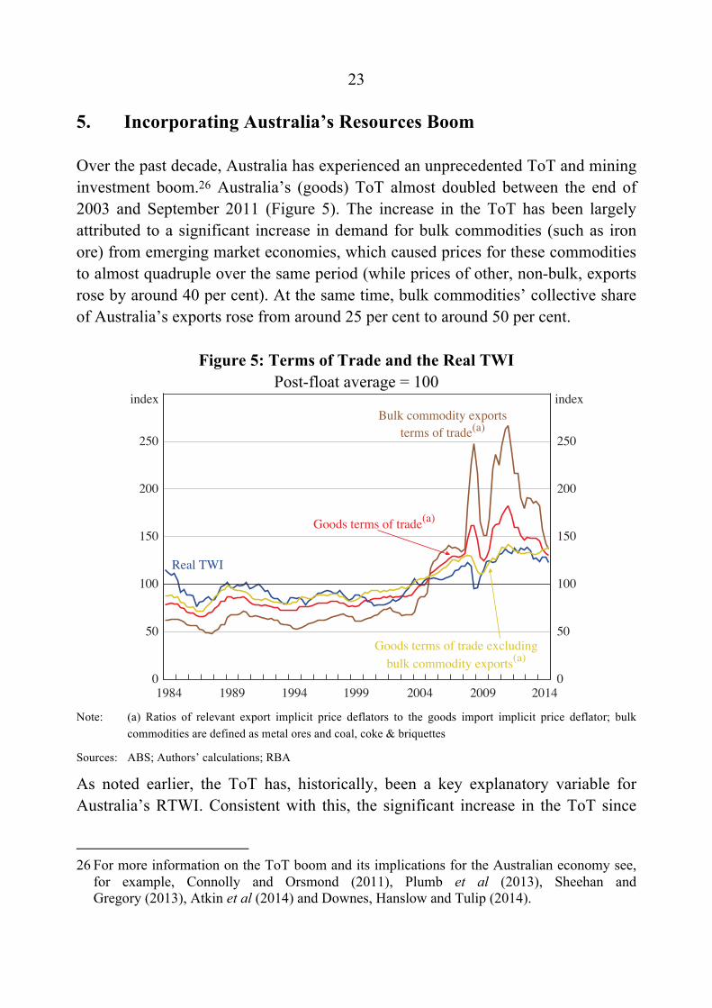
Over the past decade, Australia has experienced an unprecedented ToT and mining investment boom.26 Australia’s (goods) ToT almost doubled between the end of 2003 and September 2011 (Figure 5). The increase in the ToT has been largely attributed to a significant increase in demand for bulk commodities (such as iron ore) from emerging market economies, which caused prices for these commodities to almost quadruple over the same period (while prices of other, non-bulk, exports rose by around 40 per cent). At the same time, bulk commodities’ collective share of Australia’s exports rose from around 25 per cent to around 50 per cent.

Figure 5: Terms of Trade and the Real TWI Post-float average = 100

Note: (a) Ratios of relevant export implicit price deflators to the goods import implicit price deflator; bulk

commodities are defined as metal ores and coal, coke & briquettes


As noted earlier, the ToT has, historically, been a key explanatory variable for Australia’s RTWI. Consistent with this, the significant increase in the ToT since

26 For more information on the ToT boom and its implications for the Australian economy see,

for example, Connolly and Orsmond (2011), Plumb et al (2013), Sheehan and Gregory (2013), Atkin et al (2014) and Downes, Hanslow and Tulip (2014).

0

50

100

150

200

250

0

50

100

150

200

250

Real TWI

2014

indexindexBulk commodity exports

terms of trade(a)

Goods terms of trade(a)

200920041999199419891984

Goods terms of trade excludingbulk commodity exports(a)

24

the early 2000s also broadly coincided with an appreciation of the RTWI. However, even though changes in the prices of bulk commodity exports have driven most of the variation in the ToT in recent years, the RTWI appears, at first glance, to have had a stronger relationship with a measure of the ToT that excludes bulk commodity export prices. In particular, in recent years, the largest divergences between movements in the RTWI and in the ToT have tended to coincide with particularly large movements in the prices of bulk commodities. This observation raises two key questions:

i. Is the relationship between the RTWI and the prices of bulk commodities (as measured in the ToT) different to the relationship between the RTWI and other export prices?; and, if so

ii. Does the baseline ECM adequately capture the dynamics of the recent ToT boom, insofar as the boom was driven largely by increases in the prices of bulk commodity exports?

In Sections 5.1 and 5.2, we consider two explanations of why bulk commodity export prices could potentially have a different effect on the RTWI than other export prices and augment the baseline model in an effort to capture these differences. In broad terms, the first explanation could be that bulk commodity prices interact differently with the rest of the economy, compared with other export prices (considered in Section 5.1). The second possible explanation is that bulk commodity prices could be less reflective of current expectations than other export prices (considered in Section 5.2).

5.1 The Bulk Commodity Sector’s Interaction with the Rest of the Economy

There are at least two key reasons why bulk commodity prices could interact differently with the rest of the economy, compared to other export prices. The first is related to the extent to which the bulks industry is integrated with the rest of the economy (Section 5.1.1) and the second is related to variability in the relationship between bulks prices and investment (Section 5.1.2).

25

5.1.1 The effect of bulks prices on the rest of the economy

As discussed in Section 3.1, the theoretical literature suggests that variation in the ToT – particularly variation which is driven by changes in global supply of, and demand for, exports – should affect the RTWI. However, the magnitude of this effect is likely to differ depending on which export price(s) caused the variation (Amano and van Norden 1995). This reflects the fact that individual industries could interact differently with the rest of the economy in terms of their use of domestic inputs, their use as an input into other industries’ production, their use for domestic consumption and substitutability for other goods, and/or their overall effect on national income.

A number of papers have found empirical support for this notion. For example, both Amano and van Norden (1995) and Maier and DePratto (2008) find that a measure of the ToT which is constructed using only energy export prices has a very different relationship with the Canadian dollar’s bilateral exchange rate against the US dollar compared to a measure of the ToT which is constructed using other commodity export prices.

In an Australian context, the export sector that stands out as being potentially unique is the bulk commodities sector. Relative to other export sectors, the bulks sector, and particularly the liquefied natural gas (LNG) sub-sector, uses fewer domestic inputs for production and has a high level of foreign ownership (Connolly and Orsmond 2011; Plumb et al 2013; Rayner and Bishop 2013). Consequently, much of the additional profit associated with higher bulks prices is likely to accrue to foreigners and there will be relatively little additional demand for domestic labour associated with increased production. Overall then, a smaller proportion of the additional income associated with the rise in bulk commodity export prices will actually remain within Australia, suggesting that an increase in the price of bulk commodity exports could have a more limited effect on domestic demand, relative prices and the RTWI than an increase in other export prices (Kent 2014). Similarly, in terms of the nominal exchange rate, there may be only a small increase in net demand for Australian dollars as firms will pay their foreign owners in foreign currency.

26

If this is the case, the inclusion of bulk commodity export prices in the ToT could make it more difficult to identify a stable relationship between the ToT and the RTWI. While this may have always been an issue, it is likely to have become more prominent in recent years as bulks prices have driven an increasingly large proportion of the variation in the ToT. Decomposing the aggregate ToT into a ‘bulks ToT’ and (an ‘excluding-bulks ToT’ could help to ameliorate this issue and could provide additional insight into the behaviour of the RTWI and its relationship with different export prices.

To examine this, the bulks and excluding-bulks ToT series are included in the ECM’s cointegrating relationship separately, in place of the aggregate ToT:27

( )1 1 1 2 1 3 1

1 2 1 3 4 5 1

6 7 1 8 .

t t t t t

t t t t t

t t t t

RTWI RTWI ToTBulks ToTExBulks RIRDCRB CRB SPX VIX RTWIToTBulks ToTExBulks RIRD

µ γ β β βα α α α αα α α ε

− − − −

− −

−

Δ = + + + ++ Δ + Δ + Δ + Δ + Δ+ Δ + Δ + Δ +

(7)

Four different specifications are considered, which vary along two dimensions:

• Weighting scheme: the bulks and excluding-bulks ToT measures are calculated as both ‘unweighted’ and ‘weighted’ measures. The unweighted measures are constructed as the ratios of the bulks and excluding-bulks export price deflators to the total import price deflator. The weighted measures are constructed by multiplying the unweighted bulks and excluding-bulks ToT measures by the (time-varying) bulks and excluding-bulks nominal export shares, respectively. The weighted measures account for the increasing share of bulk commodities in Australia’s export basket over the past decade.28

• Definition of ‘bulks’: the bulks and excluding-bulks measures are calculated using two definitions of bulk commodities. The ‘narrow’ bulks measure includes only ‘metal ores’, and ‘coal, coke and briquettes’, while the ‘broad’ bulks measure also includes ‘other mineral fuels’ (e.g. LNG).

27 Unit root tests indicate that the decomposed ToT series are also non-stationary over the

sample. 28 A similar approach was used to model the Canadian dollar in Maier and DePratto (2008).

27

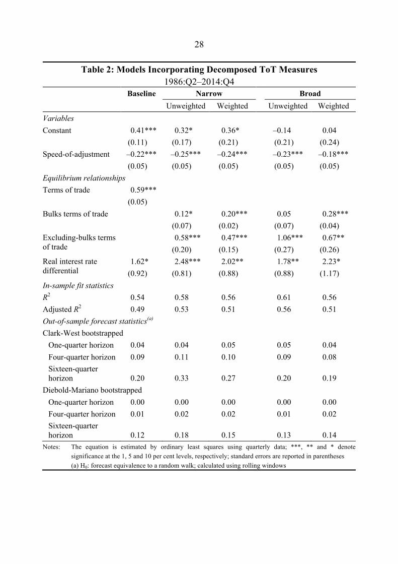
The results of these models are reported in full in Table 2. Consistent with the observation that the RTWI appears to have been less responsive to movements in bulks prices, the coefficient on the bulks ToT is significantly smaller than the coefficient on the excluding-bulks ToT in all four specifications (weighted/unweighted; broad/narrow) at the 10 per cent level (based on Wald tests). Further, the coefficient on the bulks ToT is only significant at (at least) the 5 per cent level in the two specifications that use the weighted ToT measures.

The in-sample fits of the decomposed models, as measured by the adjusted R2, are slightly higher than that of the baseline model. Their out-of-sample performances are all broadly similar to that of the baseline model in that they produce better forecasts than a random walk model (particularly at shorter horizons).29

The estimated equilibriums from all four decomposed specifications follow fairly similar paths to each other and to the baseline model for most of the sample, though they have diverged somewhat since 2003. The estimated equilibrium from the unweighted narrow and weighted broad specifications are shown below as they reflect the two extremes, both in terms of the ToT measures used and in terms of estimated equilibriums (the top panel of Figure 6 shows the unweighted narrow specification and the bottom panel shows the weighted broad specification).

29 For details on the out-of-sample forecast testing procedures, see Appendix A.

28

Table 2: Models Incorporating Decomposed ToT Measures 1986:Q2–2014:Q4

Baseline Narrow Broad Unweighted Weighted Unweighted Weighted Variables Constant 0.41*** 0.32* 0.36* –0.14 0.04 (0.11) (0.17) (0.21) (0.21) (0.24) Speed-of-adjustment –0.22*** –0.25*** –0.24*** –0.23*** –0.18*** (0.05) (0.05) (0.05) (0.05) (0.05) Equilibrium relationships Terms of trade 0.59*** (0.05) Bulks terms of trade 0.12* 0.20*** 0.05 0.28*** (0.07) (0.02) (0.07) (0.04) Excluding-bulks terms of trade

0.58*** 0.47*** 1.06*** 0.67** (0.20) (0.15) (0.27) (0.26)

Real interest rate differential

1.62* 2.48*** 2.02** 1.78** 2.23* (0.92) (0.81) (0.88) (0.88) (1.17)

In-sample fit statistics R2 0.54 0.58 0.56 0.61 0.56 Adjusted R2 0.49 0.53 0.51 0.56 0.51 Out-of-sample forecast statistics(a) Clark-West bootstrapped

One-quarter horizon 0.04 0.04 0.05 0.05 0.04 Four-quarter horizon 0.09 0.11 0.10 0.09 0.08 Sixteen-quarter horizon 0.20 0.33 0.27 0.20 0.19

Diebold-Mariano bootstrapped One-quarter horizon 0.00 0.00 0.00 0.00 0.00 Four-quarter horizon 0.01 0.02 0.02 0.01 0.02 Sixteen-quarter horizon 0.12 0.18 0.15 0.13 0.14



29

Figure 6: ‘Equilibrium’ Real TWI – Decomposed Models Post-float average = 100

Note: (a) Equilibrium is based on the model’s estimated cointegrating relationship; the SE (standard error) is the

standard deviation of the historical deviations of the RTWI from the model-implied equilibrium


The estimated equilibrium from the unweighted narrow specification follows the observed RTWI more closely over the full sample than the estimated equilibrium from the baseline model. This is demonstrated by the slightly lower standard error (SE), which is a standardised measure of the observed RTWI’s deviations from the estimated equilibrium. In particular, it tracks the RTWI more closely in 2008 and since 2013.

80

100

120

140

80

100

120

140

index

Decomposed model ‘equilibrium’term – unweighted bulks excl fuel

(SE = 6.5)(a)

60

80

100

120

140

60

80

100

120

140

2014200920041999199419891984

index

index

index

Base model ‘equilibrium’term (SE = 7.1)(a)

Real TWI

Decomposed model ‘equilibrium’term – weighted bulks incl fuel

(SE = 8.3)(a)

30

In contrast, the estimated equilibrium from the weighted broad specification diverged from the observed RTWI in 2013–14. However, given that this specification’s equilibrium has a relatively poor fit over the entire sample, as indicated by the higher SE, the estimated deviation in 2013–14 does not appear to have been especially unusual in the context of this model. While the higher SE indicates a poorer fit, it only provides a simple benchmark for assessing the models, and other factors – including the theoretical soundness of the model – should also be considered in evaluating their usefulness. In particular, this specification arguably provides the purest decomposition of the ToT into bulks and excluding-bulks (in that it encompasses the full range of bulk commodities and accounts for changing export shares).

Overall, while there is some evidence that bulk commodity export prices have a smaller effect on the RTWI than other export prices, including separate variables in the model to directly capture this has only a small effect on the models’ explanatory power over the full sample period. Moreover, including separate variables also leads to model specifications that are less parsimonious than the baseline model, and to estimated equilibriums that are quite sensitive to the exact model specification.

5.1.2 Is investment a better indicator of the effect of higher bulks prices?

As discussed above, the structure of the bulks industry means that a sizeable portion of the income associated with an increase in bulk commodity export prices will flow overseas and so the direct effect on domestic demand, relative prices and the RTWI could be relatively limited. Nevertheless, a portion of the income is still likely to flow into the domestic economy, particularly if the higher prices are accompanied by an increase in (labour-intensive) investment in the bulks sector. The increased demand for labour associated with this investment could contribute to a real appreciation of the exchange rate by: pushing up relative wages and prices; and by increasing demand for Australian dollars to pay those wages, and thereby placing upward pressure on the nominal exchange rate.

31

However, the relationship between investment in the bulks sector and developments in bulk commodity prices can be variable, both in terms of its strength and its timing, in part reflecting the ‘lumpy’ nature of investment in the mining sector. Moreover, in the recent mining investment boom, at least a portion of the investment in the LNG sub-sector is likely to have reflected factors such as technological improvements, which have made projects more viable, rather than increases in current and/or expected future prices alone.

This variability could, in turn, weaken the apparent relationship between the ToT and the RTWI during certain periods. One intuitive example of this dynamic is that, even if the ToT were to remain elevated, the exchange rate could still be expected to depreciate as the resources boom moves from its ‘investment’ phase to its (less labour-intensive) ‘production’ phase due to the associated easing in labour demand and reduction in (the growth rate of) real wages.30

These considerations suggest that investment could potentially be a better indicator of the effect of higher bulks prices on the economy – and therefore on the RTWI – than the prices themselves. To examine this, an investment-to-GDP ratio (I/GDP) variable can be added to the model’s cointegrating relationship:

( )1 1 1 2 1 3 1

1 2 1 3 4 5 1

6 7 8

/

/ .

t t t t t

t t t t t

t t t t

RTWI RTWI ToT RIRD I GDPCRB CRB SPX VIX RTWIToT RIRD I GDP

µ γ β β βα α α α αα α α ε

− − − −

− −

Δ = + + + ++ Δ + + Δ + Δ + Δ+ Δ + Δ + Δ +

(8)

30 Debelle (2014) suggests a similar dynamic. As the investment phase ends, foreign firms will

require fewer Australian dollars to pay for Australian inputs. At the same time, the increased production will not (directly) lead to much additional demand for Australian dollars as bulk commodities tend to be priced in US dollars, though there will still be some additional demand due to the higher dividends and taxes associated with increased production. Overall though, the net demand for Australian dollars is still likely to be reduced.

32

Two measures of I/GDP are considered. One is constructed using private business investment from the national accounts (Figure 7).31 The other uses a forward-looking measure of non-residential construction work yet to be done (WYTBD) (Figure 8).

Figure 7: Investment, the Terms of Trade and the Real TWI

Notes: (a) Post-float average = 100

(b) Current prices, seasonally adjusted


31 A measure of mining investment was also considered, but the estimated coefficients were

insignificant. Moreover, a likelihood ratio test suggested that including the mining investment variable did not significantly improve the fit of the model.

60

80

100

120

140

160

180

8

10

12

14

16

18

20

Real TWI(a)(LHS)

2014

%index

Investment-to-GDP ratio(b)(RHS)

Goods terms of trade(a)(LHS)

200920041999199419891984

33

Figure 8: Work Yet to be Done, the Terms of Trade and the Real TWI

Notes: (a) Post-float average = 100

(b) Current prices, seasonally adjusted


The results from incorporating the I/GDP variables into the baseline model are reported in Table 3.32 The coefficients on both investment variables are positive, as expected, but only the coefficient in the WYTBD specification is statistically significant. At the same time, the coefficient on the ToT is lower in both models (relative to the baseline ECM). This could reflect the fact that these variants of the model allow the recent investment boom to have a direct effect on the exchange rate, whereas in the baseline ECM some of its effect may have been attributed to the higher ToT (i.e. omitted variable bias). However, there is some evidence of collinearity, which makes it difficult to interpret the magnitude and significance of the individual coefficients.

32 Unit root tests indicate that both investment variables are non-stationary over the sample.

60

80

100

120

140

160

180

0

10

20

30

40

50

60

Real TWI(a)(LHS)

2014

%index

WYTBD-to-GDP ratio(b)(RHS)

Goods terms of trade(a)(LHS)

200920041999199419891984

34

Table 3: Models Incorporating Investment-to-GDP Ratios Baseline Investment WYTBD Variables Constant 0.41** 0.43*** 0.65*** (0.11) (0.11) (0.17) Speed-of-adjustment –0.22*** –0.23*** –0.24*** (0.05) (0.05) (0.05) Equilibrium relationships Terms of trade 0.59*** 0.53*** 0.39*** (0.05) (0.06) (0.09) Real interest rate differential 1.40 1.56* 1.70** (1.04) (0.90) (0.83) Total investment/GDP 1.60 (1.09) Work yet to be done/GDP 0.48** (0.21) In-sample fit statistics R2 0.51 0.56 0.59 Adjusted R2 0.48 0.51 0.54 Out-of sample forecast statistics(a) Clark-West bootstrapped

One-quarter horizon 0.04 0.04 0.05 Four-quarter horizon 0.09 0.10 0.11 Sixteen-quarter horizon 0.20 0.24 0.37

Diebold-Mariano bootstrapped One-quarter horizon 0.00 0.00 0.00 Four-quarter horizon 0.01 0.01 0.02 Sixteen-quarter horizon 0.12 0.10 0.24

Notes: The equations are estimated by ordinary least squares using quarterly data; the Baseline and Investment equations are estimated over 1986:Q2–2014:Q4, the WYTBD equation is estimated over 1986:Q4–2014:Q4; ***, ** and * denote significance at the 1, 5 and 10 per cent levels, respectively; standard errors are reported in parentheses


The models with the investment variables have slightly better in-sample fits than the baseline model; likelihood ratio tests suggest that these differences are statistically significant. Their out-of-sample forecast performance is similar to that

35

of the baseline model, though the WYTBD model performs relatively poorly at the sixteen-quarter horizon.33

The estimated equilibrium terms from these models are fairly similar to the estimated equilibrium term from the baseline ECM (Figures 9 and 10). Nevertheless, there has been some divergence in recent years. In particular, the estimated equilibrium from the models that include the investment variables have tended to be higher than the estimated equilibrium from the baseline model, reflecting the continuing high levels of investment even after the ToT declined from its peak in 2011. This also means that the equilibriums from the models which include the investment variables have tracked the observed RTWI somewhat more closely during this latter period. Nevertheless, taken as a whole, the results are not very different to those from the baseline model, which is more parsimonious.

Figure 9: ‘Equilibrium’ Real TWI – Investment Model Post-float average = 100




33 Evidence of strong exogeneity is more mixed for the WYTBD variable, suggesting that the

multi-step-ahead forecasting results should be interpreted with caution.

60

80

100

120

140

60

80

100

120

140

Real TWI

2014

indexindex

Investment model‘equilibrium’ term (SE = 7.1)(a)

Base model ‘equilibrium’ term (SE = 7.1)(a)

200920041999199419891984

36

Figure 10: ‘Equilibrium’ Real TWI – Work Yet to be Done Model Post-float average = 100




5.2 Bulk Commodity Prices and Expectations

Section 5.1 considered some reasons why the bulk commodities sector could interact differently with the economy than other sectors, which could help to explain why bulk commodity prices have a different effect on the RTWI than other export prices. A second potential reason why bulk commodity prices may have a different effect on the RTWI is that bulks prices may be less forward-looking and therefore contain less relevant information for foreign exchange market participants.

This second explanation may be important as a number of papers suggest that it is the expected path of the ToT that will affect domestic consumption, and therefore the exchange rate, through its influence on the expected path of future income (Chen et al 2010). For example, if agents expect an increase in the ToT – and the associated rise in domestic income – to be only transitory, they are likely to save a relatively high proportion of that income. In this scenario, the effect on domestic demand will be more muted than would be expected if the increase in the ToT was

60

80

100

120

140

60

80

100

120

140

Real TWI

2014

indexindex

WYTBD model ‘equilibrium’term (SE = 6.0)(a)

Base model ‘equilibrium’ term (SE = 6.9)(a)

200920041999199419891984

37

perceived to be persistent and the associated increase in income more permanent. Accordingly, we may expect a transitory ToT shock to be associated with less real appreciation pressure via the relative price channel than might be the case for a persistent ToT shock (all else equal). In a similar vein, forward-looking foreign exchange market participants should ‘price in’ expected changes in the ToT and ‘look through’ changes that are perceived to be only transitory, which suggests that there is also likely to be less nominal exchange rate appreciation than might be the case if the shock was perceived to be more long-lasting.34

There are several reasons why bulk commodity export prices, as measured in the ToT, could be less reflective of expectations of future demand and supply than other export prices. For example, until relatively recently, prices for bulk commodities were set predominantly using long-term contracts. While these contracts should incorporate expectations at the time they are set, prices are not able to react immediately to subsequent changes in the outlook for future supply and demand. In contrast, the (nominal) exchange rate is likely to respond to these changes, which could contribute to divergences between the ToT and the RTWI. This dynamic was particularly evident in late 2008, when a number of contracts for bulk commodity exports were agreed just before the onset of the (unanticipated) global financial crisis. While the nominal exchange rate – and therefore the RTWI – depreciated immediately, bulk export prices – and therefore the ToT – did not decline immediately.

More recently, the shift towards the use of shorter-term contracts and spot pricing for bulk commodities has reduced some of this price stickiness. Nevertheless, bulks prices are still likely to be less reflective of expectations than some other prices – at least periodically. This is because bulk commodities markets can be prone to transitory price spikes, reflecting relatively inelastic supply as well as the tendency for natural disasters to cause supply disruptions. Market participants and, consequently, the exchange rate are likely to ‘look through’ such price spikes, which can contribute to temporary divergences between the ToT and the RTWI. One prominent example of this dynamic occurred in 2010–11, when floods in

34 The importance of considering expectations when examining the relationship between the

ToT and the RTWI has been well documented for Australia. For example, Blundell-Wignall et al (1993) and Tarditi (1996) identify the early 1980s as a period when the RTWI appreciated in response to expected future increases in the ToT, which never eventuated.

38

Queensland pushed coal prices and the ToT higher, while the RTWI remained relatively unchanged.

Together, these factors suggest that a forward-looking measure of the ToT, which incorporates expectations for future bulk (and non-bulk) commodity export prices, could exhibit a stronger and more consistent relationship with the RTWI than the backward-looking observed ToT.

5.2.1 Is the exchange rate more responsive to a forward-looking terms of trade?

To investigate the relationship between the RTWI and the expected ToT, a number of forward-looking measures of the ToT were constructed using past vintages of the RBA’s internal goods and services ToT forecasts.35 The measures were constructed using forecast horizons of 4–8 quarters ahead for a sample beginning in 2003. The exercise assumes that the Bank’s forecasts provide a reasonable proxy for the market’s expectations for the ToT, which is, in turn, the relevant determinant of the exchange rate.36

As expected, this forward-looking ToT measure appears to track the RTWI more closely than the observed ToT (Figure 11). This is particularly evident in 2008, when both the forward-looking ToT and the RTWI appear to have declined more quickly in response to the onset of the global financial crisis than the observed ToT. Similarly, both the forward-looking ToT and the RTWI appear to have ‘looked through’ the Queensland flood-induced spike in the observed ToT in 2010–11.

35 The goods ToT is used in the baseline ECM due to concerns over endogeneity between the

RTWI and the services ToT (see Stone et al (2005) for details). However, this potential endogeneity problem will not be an issue when using forecasts for the ToT given that these forecasts are determined before the RTWI is known.

36 A time series of market forecasts for the ToT is not readily available.

39

Figure 11: Terms of Trade Forecasts and the Real TWI March quarter 2003 = 100


In order to formally test the relationship between expectations for the ToT and the RTWI, various forward-looking ToT measures (FToTs) are included in the cointegrating relationship of the baseline model in place of the observed ToT:37

( )1 1 1 2 1 1 2 1

3 4 5 1 6 7 .t t t t t t

t t t t t t

RTWI RTWI FToT RIRD CRB CRBSPX VIX RTWI FToT RIRD

µ γ β β α αα α α α α ε

− − − −

−

Δ = + + + + Δ + Δ+ Δ + Δ + Δ + Δ + Δ +

(9)

The results from the model that includes an eight-quarter-ahead ToT forecast variable are reported in Table 4 (other forecast horizons were also considered, with similar results). As expected, when both models are estimated over a sample beginning in 2003, the speed-of-adjustment coefficient from the forward-looking model is larger (in absolute terms) than the speed-of-adjustment coefficient from the baseline model, suggesting that the RTWI responds more quickly to changes in

37 Unit root tests indicate that the FToTs are non-stationary over the sample.

80

100

120

140

160

180

200

80

100

120

140

160

180

200

Real TWI

2014

indexindex

Goods and servicesterms of trade

Goods terms of trade

20122010200820062004

Eight-quarter-ahead forecastgoods and services terms of trade

40

the FToT than the observed ToT.38 The in-sample fit of both the baseline and the eight-quarter-ahead models is similar.39

Table 4: Model Incorporating a Forward-looking ToT Measure 2003:Q1–2014:Q4

Baseline Eight-quarter-ahead Variables Constant 0.55*** 0.66*** (0.15) (0.15) Speed-of-adjustment –0.24*** –0.48*** (0.06) (0.11) Equilibrium relationships Terms of trade 0.50*** 0.72*** (0.07) (0.05) Real interest rate differential 1.24 0.28 (1.93) (0.91) In-sample fit statistics R2 0.85 0.87 Adjusted R2 0.82 0.84 Notes: The equation is estimated by ordinary least squares using quarterly data; ***, ** and * denote

significance at the 1, 5 and 10 per cent levels, respectively; standard errors are reported in parentheses

The estimated equilibrium from the FToT model tracks the observed RTWI more closely than the estimated equilibrium from the baseline model (when it is estimated over the same shorter sample period), as evidenced by the smaller SE (Figure 12). This is particularly evident in 2008 and also between 2012 and end 2014. Overall, the results suggest that the RTWI may display a more robust relationship with a forward-looking measure of the ToT, albeit over a significantly shorter sample period than the baseline model.

38 Illustrative analysis suggests that this is also the case when the other short-run dynamics are

included. 39 Out-of-sample forecast statistics were not calculated due to the short length of the sample.

41

Figure 12: ‘Equilibrium’ Real TWI – Forward-looking Terms of Trade Model

Notes: (a) March quarter 2003 = 100

(b) Equilibrium is based on the model’s estimated cointegrating relationship; the SE (standard error) is the standard deviation of the historical deviations of the RTWI from the model-implied equilibrium


6. Incorporating Unconventional Monetary Policy

In addition to the resources boom, another recent macroeconomic development that may help to identify additional relevant explanatory variables has been the implementation of unconventional monetary policy by a number of major advanced economy central banks – including quantitative easing and explicit forward guidance. A key objective of these actions has been to lower longer-term bond yields as policy rates have approached (and even moved slightly below) zero. This objective appears to have been met; for example, a GDP-weighted average of real yields on US, Japanese and German 10-year government securities declined by around 200 basis points between mid 2009 and end 2014, whereas a similar measure constructed using real policy rates was broadly unchanged over the same period (Figure 13).

85

100

115

130

145

160

85

100

115

130

145

160

Real TWI(a)

2014

indexindex

Eight-quarter-ahead forecast model‘equilibrium’ term (SE = 4.0)(b)

Base model ‘equilibrium’ term (SE = 7.5)(b)

20122010200820062004

42

Figure 13: G3 and Australian Real Interest Rate Differentials Deflated using year-ended CPI inflation

Note: Weighted by PPP GDP

Sources: Authors’ calculations; Bloomberg; CEIC Data; Global Financial Data; RBA; Thomson Reuters

In addition to the effect of unconventional monetary policy on longer-term bond yields in the countries concerned, a number of papers have documented the influence of these actions on global asset prices.40 Of particular interest, Bauer and Neely (2014) and Neely (2014) find evidence that the US Federal Reserve’s unconventional monetary policy actions led to lower yields on Australian Government securities (AGS) and to an appreciation of the Australian dollar against the US dollar.

The papers usually point to two main channels through which these effects are propagated:

• the signalling channel, which operates via the effect of unconventional monetary policy on the market’s expected future path of (domestic and, potentially, foreign) short-term interest rates;

40 See for example: Bauer and Neely (2014); Neely (2014); Rogers, Scotti and Wright (2014);

and Bowman, Londono and Sapriza (2014).

-3

0

3

6

9Australia

2014-3

0

3

6

9

Policy rates ppt10-year government bond yieldsppt

20021990201420021990

G3(a)Rate

differential

43

• the portfolio balance channel, which operates via the effect of central bank asset purchases on the prices of those assets. This can lead investors to substitute towards alternative assets, including foreign assets, in turn pushing up a broader range of asset prices. If this substitution involves cross-border capital flows, there can be implications for exchange rates.

However, the baseline ECM of the RTWI is unlikely to adequately capture these dynamics. This is because the model’s RIRD variable is based on policy rates, whereas unconventional monetary policy is more likely to be evident through its effect on longer-term interest rates. In an attempt to better capture these dynamics, we present a number of augmented versions of the existing model that incorporate alternative RIRD measures.41 To this end, two model variations are presented: (i) models that replace the real policy rate differential variable with a longer-term RIRD (Section 6.1); and (ii) models that include information on both short- and long-term RIRDs (Section 6.2). Importantly, only specifications that can be estimated over the same sample period as the existing model are considered (1986 onward). Consequently, a number of alternative RIRD measures – particularly those based on measures of expected inflation – are excluded owing to data availability constraints.

Although a range of interest rates could be used to calculate longer-term RIRDs, we focus on 10-year yields on government securities for consistency with previous work. The results are nevertheless broadly similar if government debt securities of shorter maturities are used instead (e.g. 2-year or 5 year tenors), and if government bond yields are replaced with swap rates. A more fundamental issue, though, is the choice of which inflation measure to use to deflate nominal yields. When assessing investments, the relevant consideration for forward-looking market participants is expected inflation over the investment horizon. Nevertheless, past papers have tended to use observed inflation over the previous year, which implicitly assumes that inflation expectations are highly adaptive (Gruen and Wilkinson 1991; Blundell-Wignall et al 1993). Although inflation over the previous year could be a reasonable measure of inflation expectations for the near-term – and could

41 One other approach that was considered, but which is not reported in detail as the estimated

coefficient was not significant, is to use ‘shadow rates’, as reported in Wu and Xia (2014), in place of policy rates. Shadow rates are estimates of the short-term rate that would be associated with the stance of monetary policy, if the zero lower bound was not binding.

44

therefore be deemed an acceptable deflator for short-term interest rates – it is less likely to reflect inflation expectations over longer horizons.

To address this, a ‘forward-looking’ 10-year RIRD measure is also constructed. This measure uses expectations implied by 10-year inflation-linked government securities as the measure of Australian inflation expectations, and the Federal Reserve Bank of Cleveland’s survey-based measure of expected inflation over the next 10 years as the measure of US inflation expectations.42

6.1 Policy Rates and Longer-term Rates

Past RBA work has found RIRDs based on longer-term interest rates to be significant determinants of the RTWI, (Gruen and Wilkinson 1991; Blundell-Wignall et al 1993). This is consistent with the forward-looking nature of foreign exchange markets. For example, assuming that the expectations hypothesis holds, if market participants believe that a country’s central bank has shifted to an easing bias and will soon begin to reduce its policy rate, longer-term rates should decline and the exchange rate would generally be expected to depreciate even though the observed policy rate will initially remain unchanged.

To examine this, models which include 10-year RIRD measures instead of the real policy rate differential were estimated. The results are not reported as the estimated coefficients on the 10-year RIRD measures are negative and statistically insignificant, which is counterintuitive.

42 Liquidity and other issues in the market for Australian inflation-linked government securities

could distort the measure of inflation expectations. However, an alternative measure is not available over a sufficient sample. Further, while there could be issues in comparing a market-implied measure (as used for Australia) with a survey measure (as used for the United States), a sufficient time series on US inflation-linked securities was not available. Adequate time series data on Japanese and German inflation expectations are also not available.

45

One possible explanation for the unexpected negative (and insignificant) coefficients could be the presence of time-varying sovereign ‘risk premia’, which also affect the exchange rate.43 A decline in such a premium is tantamount to an outwards shift in the demand curve for government debt in that, all else equal, it would lead to higher prices, lower yields and therefore a lower RIRD. However, this lower RIRD is unlikely to be associated with a depreciation of the exchange rate. In fact, if the decline in the risk premium entices foreign investors to purchase additional securities (or domestic investors to shift from foreign to domestic securities) the lower RIRD could even be associated with a local currency appreciation.

This type of dynamic may have been evident in Australia in recent years, as foreign investors have increased their holdings of AGS.44 Further, it is broadly consistent with the portfolio balance channel of unconventional monetary policy transmission. If such a dynamic has been at play, it will make it more difficult to identify a stable relationship between longer-term RIRDs and the exchange rate. For example, a given increase in the RIRD could reflect either an increase in the risk premium (which would be expected to be associated with, if anything, a depreciation of the RTWI) or an increase in expected interest rates (which would be expected to be associated with an appreciation of the RTWI), or a combination of the two.

6.2 Long- and Short-term Real Interest Rate Differentials

Tarditi (1996) suggests that interest rate differential measures that are based on the slopes of yield curves are likely to provide more explanatory power than measures that are based only on short- or longer-term interest rates. This is because the slope of the yield curve captures both the current stance of monetary policy and the anticipated path of future short-term rates. To examine this, we estimated a number

43 Kaminska, Meldrum and Smith (2013) find that a time-varying ‘foreign exchange risk

premium’ plays a role in determining exchange rates. In this paper, ‘risk premiums’ is a broad term that encompasses a number of factors, including term premiums and credit spreads. These factors are influenced both by investor expectations and changes in investors’ preferences and/or risk aversion.

44 Models that directly incorporate foreign holdings of AGS were also considered. Neither the level of, nor the change in, foreign holdings of AGS were found to be significant determinants of the RTWI.

46

of models that include nominal and real slope differentials instead of the real policy rate differential. Consistent with Tarditi (1996), the estimated coefficients on the slope differentials were negative and statistically significant in all variations. This suggests that a flattening of the Australian yield curve relative to the foreign yield curve has – over the medium term – been associated with an appreciation of the RTWI. Nevertheless, the results are difficult to interpret because changes in the slope of the yield curve can be driven by movements in shorter- and/or longer-term interest rates, with quite different implications for the RTWI depending on the relative contributions of each.

To address this, short- and long-term real rate differentials can instead be allowed to enter the model separately. This can be interpreted as allowing changes in current and/or expected short-term interest rates (proxied using the 2-year government bond yield differential) and in risk premiums (proxied using longer-term rate differentials) to affect the RTWI in different ways. It can also be thought of as allowing the model to separately incorporate the influence of unconventional monetary policy that is transmitted via the signalling channel – often identified in the literature using shorter-term rates – and via the portfolio balance channel – often identified in the literature using longer-term rates (e.g. Rogers et al 2014).

Two specifications are reported. The first – which is subsequently referred to as the ‘backward-looking’ model – includes the 10-year RIRD between Australia and the G3 economies and the 2-year RIRD between Australia and the G3, with all rates deflated using the prior year’s inflation rate. The second – subsequently referred to as the ‘forward-looking’ model – includes the 10-year RIRD between Australia and the United States, deflated using measures of inflation expectations, and the 2-year rate differential between Australia and the United States, deflated using previous-year inflation:45

ΔRTWIt = µ + γ RTWIt−1 + β1ToTt−1 + β210yrRIRDt−1 + β2 2yrRIRDt−1( )+α1ΔCRBt +α 2ΔCRBt−1 +α3ΔSPXt +α 4ΔVIXt +α5ΔRTWIt−1

+α6ΔToTt +α7Δ10yrRIRDt +α7Δ2yrRIRDt + ε t . (10)

45 The 2-year rate is used instead of the policy rate as it is deemed to be more likely to capture

the ‘signalling’ channel.

47

The results are reported in Table 5.46 To summarise, the coefficient on the 2-year rate differential is positive and significant in both models, while the coefficient on the 10-year rate differential is negative and significant. The fact that the coefficients on the individual 2-year and 10-year rate differentials become significant when both variables are included in the model suggests that there may be an omitted variable bias in the models that include only one of the variables. Meanwhile, the in-sample and out-of-sample fits of the models with two RIRD variables are similar to that of the baseline model.

It is worth noting that the high degree of positive correlation between the 2-year and 10-year rates means that the estimates of these coefficients are likely to be affected by collinearity, which makes it difficult to interpret the individual coefficients. In turn, this may help to explain the relatively large magnitudes of the two estimated RIRD coefficients. However, given the estimated coefficients have opposite signs, the model will net off the two effects when estimating the overall impact of interest rates on the equilibrium RTWI.

The estimated equilibrium terms from both the backward- and forward-looking models are also similar to the baseline model’s estimated equilibrium (Figure 14). However, the estimated equilibrium from the forward-looking model has been a bit higher than the equilibrium from the baseline model in recent years, and has therefore tended to track movements in the observed RTWI somewhat more closely over this period. While this provides some tentative evidence that unconventional monetary policy in the major advanced economies has had some effect on the RTWI over recent years, it does not result in a significant improvement in the overall fit of the model over the entire sample period.

46 Unit root tests indicate that the 2-year and 10-year RIRDs are non-stationary over the sample

period.

48

Table 5: Models Including Short- and Long-term RIRDs 1986:Q2–2014:Q4

Baseline Backward-looking Forward-looking Variables Constant 0.41*** 0.40*** 0.44*** (0.11) (0.12) (0.12) Speed-of-adjustment –0.22*** –0.19*** –0.22*** (0.05) (0.05) (0.05) Equilibrium relationships Terms of trade 0.59*** 0.52*** 0.57*** (0.05) (0.06) (0.05) Real interest rate differential – short-term

1.62* 6.87** 1.35* (0.92) (3.18) (0.76)

Real interest rate differential – long-term

–7.38* –4.63*** (3.37) (2.31)

In-sample fit statistics R2 0.54 0.55 0.53 Adjusted R2 0.49 0.50 0.49 Out-of-sample forecast statistics(a) Clark-West bootstrapped

One-quarter horizon 0.04 0.05 0.07 Four-quarter horizon 0.09 0.10 0.12 Sixteen-quarter horizon 0.20 0.21 0.28

Diebold-Mariano bootstrapped One-quarter horizon 0.00 0.00 0.00 Four-quarter horizon 0.01 0.03 0.03 Sixteen-quarter horizon 0.12 0.10 0.19



49

Figure 14: ‘Equilibrium’ Real TWI – Short- and Long-term RIRDs Models 2-year and 10-year RIRDS, post-float average = 100




7. Conclusion

This paper has presented an error correction model of the Australian dollar real exchange rate that has displayed robust explanatory power for a number of decades, as well as a range of augmented versions of this model. The rolling error correction model and Markov-switching variations have examined whether the relationship between the real exchange rate and the baseline model’s existing

80

100

120

140

80

100

120

140

index

‘Backward-looking’ model‘equilibrium’ term (SE = 8.4)(a)

60

80

100

120

140

60

80

100

120

140

2014200920041999199419891984

index

index

index

Base model ‘equilibrium’term (SE = 7.1)(a)

Real TWI

‘Forward-looking’ model ‘equilibrium’ term(SE = 7.1)(a)

50

explanatory variables have changed significantly over time. A second set of variations have examined whether two recent important macroeconomic developments – namely, the resources boom and foreign central banks’ unconventional monetary policy actions – may have helped to identify additional medium-term determinants of the exchange rate.

Taken as a whole, while the results from these augmented models support the notion that there have been some additional influences on the real exchange rate in recent years, they do not fully account for the behaviour of the exchange rate during the period. Moreover, it is difficult to quantify these influences definitively, as even though each of the model specifications considered can be justified a priori based on theory, they produce a range of estimated equilibrium paths for the real exchange rate. Further, objective measures of in- and out-of-sample fit do not suggest that any single model’s explanatory power is clearly superior to the others, or even to that of the baseline model, over the entire sample period.

This exemplifies the imprecise nature of exchange rate modelling, which is well established in the literature. Choices regarding the modelling framework, the explanatory variables and even the sample period will all influence the models’ results. Consequently, it is difficult to conclude that any single model is the ‘true’ model of the exchange rate, or even the ‘best’ model of the exchange rate, and therefore to conclude that any estimated level of the exchange rate is the ‘appropriate’ level. Instead, such assessments will inevitably require a degree of judgement, incorporating a broader analysis of a range of other economic variables.

51

Appendix A: Out-of-sample Forecasting

In assessing the models’ out-of-sample performance, actual realised values of the explanatory variables are used to construct forecasts of the RTWI at different horizons. Test statistics are then constructed by comparing these forecasts to the realised values of the RTWI.

Consistent with a large portion of the literature, the structural models are compared to a naïve forecast model, namely a random walk. This is done using the DM (Diebold and Mariano 1995; West 1996) and CW statistics (Clark and West 2006, 2007), both of which assess models based on their mean squared forecast errors (MSFE).

The CW statistic is widely used in assessing the out-of-sample performance of nested models.47 The CW statistic compares the MSFE of the two models but, unlike a number of other test statistics, it accounts for a bias in the MSFE that arises when comparing nested models. The intuition behind this adjustment is that, if the true data-generating process is a random walk, the structural model is over-fitted, which can reduce its forecast accuracy and lead to a higher MSFE. This issue would be ameliorated if the sample was sufficiently large, as the estimate of the structural model should approach the true random walk model. However, in most cases the sample will not be sufficiently large and the small-sample bias will remain (Clark and West 2006).

The CW statistic therefore compares the MSFE of the random walk model to the adjusted MFSE of the structural model.48 If the forecasts tend not to be biased, the null hypothesis is that the two models have equivalent forecast performance and the test can be considered to be a minimum MSFE test.49 A CW statistic of zero would then indicate equivalent forecast performance, while a CW statistic above zero would indicate that the structural model’s forecasts are ‘better’ than those from the random walk model (Rogoff and Stavrakeva 2008). However, if the forecasts are biased, the null hypothesis is that the exchange rate is a random walk 47 A model is nested in another model if it can be seen as a special case of the more general

model (i.e. if it can be obtained by applying restrictions to the parameters of the general model).

48 Clark and West (2007) extend this to the case where the nested model is not a random walk. 49 ‘Bias’ refers to scale bias, not location bias. See Rogoff and Stavrakeva (2008) for details.

52

and the test can no longer be considered a test of minimum MSFE (Rogoff and Stavrakeva 2008).

Comparing the MSFE of the random walk to that of the structural models remains a valid question even if the ‘true’ model is something other than a random walk. For this reason the DM statistic is also considered, as it compares the ‘raw’– or unadjusted – root MSFE from the structural model directly to that of the naïve random walk model. A DM statistic greater than zero (less than zero) indicates that the structural model has a lower (higher) MSFE and so produces superior (inferior) forecasts, compared to the random walk model.

While both the CW and DM statistics have standard normal asymptotic distributions, bootstrapped distributions are also constructed given the small sample size. Distributions for the CW and DM statistics are constructed using a semi-parametric residual bootstrapping technique. The technique closely follows that of Mark and Sul (2001), which is also employed in a number of other papers, including Rogoff and Stavrakeva (2008). The p-values for both the CW and DM statistics are defined as the proportion of the distribution above the ‘observed’ statistic.

The out-of-sample assessment is conducted on the baseline model, the four decomposed ToT specifications, the two I/GDP models, and the two models that include short- and long-term RIRD.50 Rolling windows are used, consistent with much of the literature, with a window length of 70 quarters.51 The statistics are calculated for forecast horizons of one, four and sixteen quarters, and are reported in Tables A1 and A2.

One drawback of this bootstrapping technique, and relatedly the method for calculating the forecast statistics, is that it involves estimating the cointegrating relationship over the full sample period. As a result, information from the full sample is used in constructing the forecasts, which could provide the structural models with an ‘unfair’ advantage. Therefore, as a robustness check, bootstrapped distributions are also constructed using a fairly standard residual bootstrap, and

50 Out-of-sample testing could not be carried out on the FToT model due to the short sample. 51 As a robustness check, the out-of-sample forecast testing was also carried out using recursive

regressions. The results were broadly similar and are therefore not reported.

53

carried out under the null hypothesis of no predictability.52 This approach involves estimating the cointegrating relationship over rolling windows, rather than over the full sample, when constructing the forecast statistics and their bootstrapped distributions. Alquist and Chinn (2008) contend that estimating the cointegrating relationship over rolling windows should ensure that the forecasts are true ex ante predictions and should make the hypothesis tests more stringent.

Table A1: CW – Rolling Windows with Short- and Long-run Variables Cointegrating relationship estimated over full sample

Horizon One-quarter Four-quarter Sixteen-quarter

CW p-value(a) p-value(b) CW p-value(a) p-value(b) CW p-value(a) p-value(b) Baseline 1.96 0.03 0.04 2.23 0.01 0.09 3.10 0.00 0.20 Unweighted narrow 1.97 0.02 0.04 2.03 0.02 0.11 1.93 0.03 0.33 Weighted narrow 1.98 0.02 0.05 2.14 0.02 0.10 2.49 0.01 0.27 Unweighted broad 1.96 0.02 0.05 2.20 0.01 0.09 3.19 0.00 0.20 Weighted broad 1.96 0.03 0.04 2.32 0.01 0.08 3.28 0.00 0.19 Investment 1.97 0.02 0.04 2.11 0.02 0.10 2.89 0.00 0.24 WYTBD 1.80 0.04 0.05 1.94 0.03 0.11 1.27 0.10 0.37 Backward-looking RIRD 2.02 0.02 0.05 2.19 0.01 0.12 3.14 0.00 0.21 Forward-looking RIRD 1.81 0.03 0.07 1.98 0.02 0.10 2.48 0.01 0.28 Notes: (a) Using standard normal distribution (b) Using bootstrapped distribution

52 This method does not impose cointegration. Therefore, it could also be useful in identifying

whether the imposition of cointegration as part of the first bootstrapping methodology leads to a bias in the results.

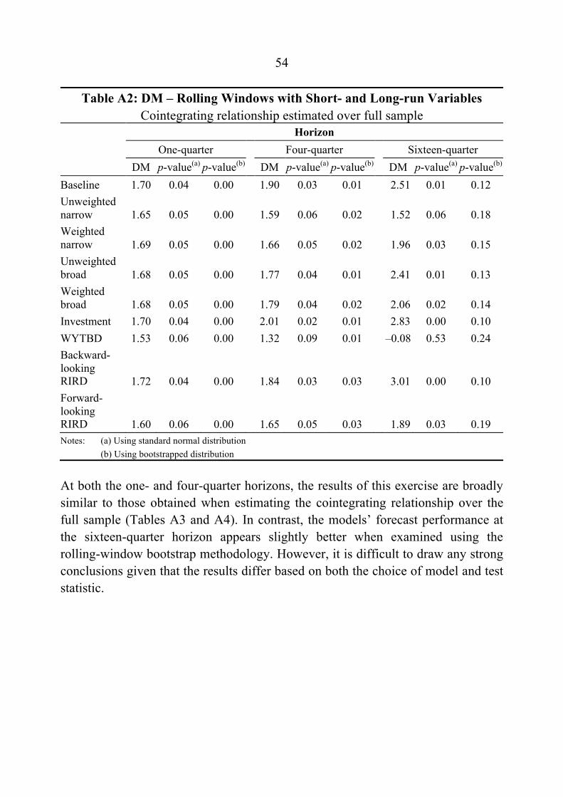
54

Table A2: DM – Rolling Windows with Short- and Long-run Variables Cointegrating relationship estimated over full sample


DM p-value(a) p-value(b) DM p-value(a) p-value(b) DM p-value(a) p-value(b) Baseline 1.70 0.04 0.00 1.90 0.03 0.01 2.51 0.01 0.12 Unweighted narrow 1.65 0.05 0.00 1.59 0.06 0.02 1.52 0.06 0.18 Weighted narrow 1.69 0.05 0.00 1.66 0.05 0.02 1.96 0.03 0.15 Unweighted broad 1.68 0.05 0.00 1.77 0.04 0.01 2.41 0.01 0.13 Weighted broad 1.68 0.05 0.00 1.79 0.04 0.02 2.06 0.02 0.14 Investment 1.70 0.04 0.00 2.01 0.02 0.01 2.83 0.00 0.10 WYTBD 1.53 0.06 0.00 1.32 0.09 0.01 –0.08 0.53 0.24 Backward-looking RIRD 1.72 0.04 0.00 1.84 0.03 0.03 3.01 0.00 0.10 Forward-looking RIRD 1.60 0.06 0.00 1.65 0.05 0.03 1.89 0.03 0.19 Notes: (a) Using standard normal distribution (b) Using bootstrapped distribution

At both the one- and four-quarter horizons, the results of this exercise are broadly similar to those obtained when estimating the cointegrating relationship over the full sample (Tables A3 and A4). In contrast, the models’ forecast performance at the sixteen-quarter horizon appears slightly better when examined using the rolling-window bootstrap methodology. However, it is difficult to draw any strong conclusions given that the results differ based on both the choice of model and test statistic.

55

Table A3: CW – Rolling Windows with Short- and Long-run Variables Cointegrating relationship re-estimated in each sample


CW p-value(a) p-value(b) CW p-value(a) p-value(b) CW p-value(a) p-value(b) Baseline 2.07 0.02 0.03 2.17 0.01 0.09 2.74 0.00 0.18 Unweighted narrow 2.09 0.02 0.03 2.12 0.02 0.09 3.20 0.00 0.08 Weighted narrow 2.03 0.02 0.03 1.91 0.03 0.11 2.19 0.01 0.25 Unweighted broad 1.98 0.04 0.04 2.43 0.01 0.04 3.49 0.00 0.03 Weighted broad 1.79 0.04 0.05 2.16 0.02 0.05 1.91 0.03 0.23 Investment 2.15 0.02 0.03 2.33 0.01 0.06 2.78 0.00 0.17 WYTBD 2.38 0.01 0.02 2.20 0.01 0.05 3.45 0.00 0.06 Backward-looking RIRD 2.10 0.02 0.02 2.05 0.02 0.08 2.30 0.01 0.15 Forward-looking RIRD 2.08 0.02 0.02 2.11 0.02 0.07 3.00 0.00 0.12 Notes: (a) Using standard normal distribution (b) Using bootstrapped distribution

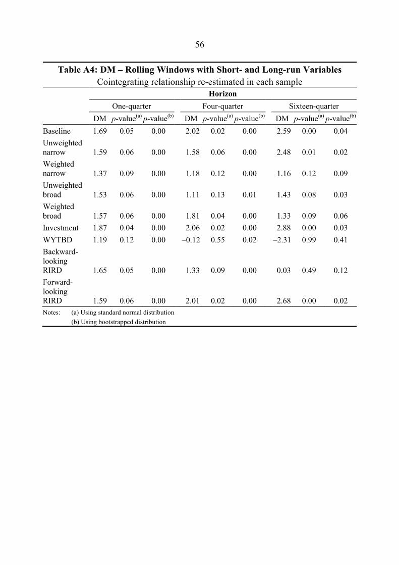
56

Table A4: DM – Rolling Windows with Short- and Long-run Variables Cointegrating relationship re-estimated in each sample


DM p-value(a) p-value(b) DM p-value(a) p-value(b) DM p-value(a) p-value(b) Baseline 1.69 0.05 0.00 2.02 0.02 0.00 2.59 0.00 0.04 Unweighted narrow 1.59 0.06 0.00 1.58 0.06 0.00 2.48 0.01 0.02 Weighted narrow 1.37 0.09 0.00 1.18 0.12 0.00 1.16 0.12 0.09 Unweighted broad 1.53 0.06 0.00 1.11 0.13 0.01 1.43 0.08 0.03 Weighted broad 1.57 0.06 0.00 1.81 0.04 0.00 1.33 0.09 0.06 Investment 1.87 0.04 0.00 2.06 0.02 0.00 2.88 0.00 0.03 WYTBD 1.19 0.12 0.00 –0.12 0.55 0.02 –2.31 0.99 0.41 Backward-looking RIRD 1.65 0.05 0.00 1.33 0.09 0.00 0.03 0.49 0.12 Forward-looking RIRD 1.59 0.06 0.00 2.01 0.02 0.00 2.68 0.00 0.02 Notes: (a) Using standard normal distribution (b) Using bootstrapped distribution

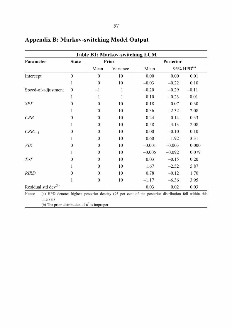
57

Appendix B: Markov-switching Model Output

Table B1: Markov-switching ECM Parameter State Prior Posterior Mean Variance Mean 95% HPD(a) Intercept 0 0 10 0.00 0.00 0.01 1 0 10 –0.03 –0.22 0.10 Speed-of-adjustment 0 –1 1 –0.20 –0.29 –0.11 1 –1 1 –0.10 –0.23 –0.01 SPX 0 0 10 0.18 0.07 0.30 1 0 10 –0.36 –2.32 2.08 CRB 0 0 10 0.24 0.14 0.33 1 0 10 –0.58 –3.13 2.08 CRBt – 1 0 0 10 0.00 –0.10 0.10 1 0 10 0.60 –1.92 3.31 VIX 0 0 10 –0.001 –0.003 0.000 1 0 10 –0.005 –0.092 0.079 ToT 0 0 10 0.03 –0.15 0.20 1 0 10 1.67 –2.52 5.87 RIRD 0 0 10 0.78 –0.12 1.70 1 0 10 –1.17 –6.36 3.95 Residual std dev(b) 0.03 0.02 0.03 Notes: (a) HPD denotes highest posterior density (95 per cent of the posterior distribution fell within this

interval) (b) The prior distribution of σ2 is improper

58

References

Alquist R and MD Chinn (2008), ‘Conventional and Unconventional Approaches to Exchange Rate Modelling and Assessment’, International Journal of Finance & Economics, 13(1), pp 2–13.

Amano RA and S van Norden (1995), ‘Terms of Trade and Real Exchange Rates: The Canadian Evidence’, Journal of International Money and Finance, 14(1), pp 83–104.

Atkin T, M Caputo, T Robinson and H Wang (2014), ‘Macroeconomic Consequences of Terms of Trade Episodes, Past and Present’, RBA Research Discussion Paper No 2014-01.

Balassa B (1964), ‘The Purchasing Power Parity Doctrine: A Reappraisal’, Journal of Political Economy, 72(6), pp 584–596.

Banerjee A, JJ Dolado, DF Hendry and GW Smith (1986), ‘Exploring Equilibrium Relationships in Econometrics through Static Models: Some Monte Carlo Evidence’, Oxford Bulletin of Economics and Statistics, 48(3), pp 253–277.

Bauer MD and C Neely (2014), ‘International Channels of the Fed’s Unconventional Monetary Policy’, Journal of International Money and Finance, 44, pp 24–46.

Beaumont C and L Cui (2007), ‘Conquering the Fear of Floating—Australia’s Successful Adaptation to a Flexible Exchange Rate’, IMF Policy Discussion Paper PDP/07/02.

Beechey M, N Bharucha, A Cagliarini, D Gruen and C Thompson (2000), ‘A Small Model of the Australian Macroeconomy’, RBA Research Discussion Paper No 2000-05.

Bewley RA (1979), ‘The Direct Estimation of the Equilibrium Response in a Linear Dynamic Model’, Economics Letters, 3(4), pp 357–361.

59

Blundell-Wignall A, J Fahrer and A Heath (1993), ‘Major Influences on the Australian Dollar Exchange Rate’, in A Blundell-Wignall (ed), The Exchange Rate, International Trade and the Balance of Payments, Proceedings of a Conference, Reserve Bank of Australia, Sydney, pp 30–78.

Blundell-Wignall A and RG Gregory (1990), ‘Exchange Rate Policy in Advanced Commodity-Exporting Countries: The Case of Australia and New Zealand’, OECD Economics Department Working Papers No 83.

Bowman D, JM Londono and H Sapriza (2014), ‘U.S. Unconventional Monetary Policy and Transmission to Emerging Market Economies’, Board of Governors of the Federal Reserve System International Finance Discussion Paper No 1109.

Cashin P, LF Céspedes and R Sahay (2004), ‘Commodity Currencies and the Real Exchange Rate’, Journal of Development Economics, 75(1), pp 239–268.

Catão LAV and R Chang (2013), ‘World Food Prices, the Terms of Trade-Real Exchange Rate Nexus, and Monetary Policy’, IMF Working Paper WP/13/114.

Cayen J-P, D Coletti, R Lalonde and P Maier (2010), ‘What Drives Exchange Rates? New Evidence from a Panel of U.S. Dollar Bilateral Exchange Rates’, Bank of Canada Working Paper 2010-5.

Chen Y and K Rogoff (2003), ‘Commodity Currencies’, Journal of International Economics, 60(1), pp 133–160.

Chen Y, K Rogoff and B Rossi (2010), ‘Can Exchange Rates Forecast Commodity Prices?’, The Quarterly Journal of Economics, 125(3), pp 1145–1194.

Cheung Y-W, MD Chinn and AG Pascual (2005), ‘Empirical Exchange Rate Models of the Nineties: Are any Fit to Survive?’, Journal of International Money and Finance, 24(7), pp 1150–1175.

60

Clark PB and R MacDonald (1999), ‘Exchange Rates and Economic Fundamentals: A Methodological Comparison of BEERs and FEERs’, in R MacDonald and JL Stein (eds), Equilibrium Exchange Rates, Recent Economic Thought, Vol 69, Springer Science+Business Media, New York, pp 285–322.

Clark TE and KD West (2006), ‘Using Out-Of-Sample Mean Squared Prediction Errors to Test the Martingale Difference Hypothesis’, Journal of Econometrics, 135(1–2), pp 155–186.

Clark TE and KD West (2007), ‘Approximately Normal Tests for Equal Predictive Accuracy in Nested Models’, Journal of Econometrics, 138(1), pp 291–311.

Connolly E and D Orsmond (2011), ‘The Mining Industry: From Bust to Boom’, RBA Research Discussion Paper No 2011-08.

De Grauwe P and M Grimaldi (2006), ‘Exchange Rate Puzzles: A Tale of Switching Attractors’, European Economic Review, 50(1), pp 1–33.

Debelle G (2014), ‘Capital Flows and the Australian Dollar’, Speech to the Financial Services Institute of Australia, Adelaide, 20 May.

Debelle G and M Plumb (2006), ‘The Evolution of Exchange Rate Policy and Capital Controls in Australia’, Asian Economic Papers, 5(2), pp 7–29.

Diebold FX (2015), ‘Comparing Predictive Accuracy, Twenty Years Later: A Personal Perspective on the Use and Abuse of Diebold-Mariano Tests’, Journal of Business & Economic Statistics, 33(1), pp 1–9.

Diebold FX and RS Mariano (1995), ‘Comparing Predictive Accuracy’, Journal of Business & Economic Statistics, 13(3), pp 253–263.

Dornbusch R (1976), ‘Expectations and Exchange Rate Dynamics’, Journal of Political Economy, 84(6), pp 1161–1176.

Dornbusch R (1980), Open Economy Macroeconomics, Basic Books, New York.

61

Downes P, K Hanslow and P Tulip (2014), ‘The Effect of the Mining Boom on the Australian Economy’, RBA Research Discussion Paper No 2014-08.

Driver RL and PF Westaway (2004), ‘Concepts of Equilibrium Exchange Rates’, Bank of England Working Paper No 248.

Dvornak N, M Kohler and G Menzies (2003), ‘Australia’s Medium-Run Exchange Rate: A Macroeconomic Balance Approach’, RBA Research Discussion Paper No 2003-03.

Dwyer J and P Lowe (1993), ‘Alternative Concepts of the Real Exchange Rate: A Reconciliation’, RBA Research Discussion Paper No 9309.

Engel C (1994), ‘Can the Markov Switching Model Forecast Exchange Rates?’, Journal of International Economics, 36(1–2), pp 151–165.

Engle RF and CWJ Granger (1987), ‘Co-Integration and Error Correction: Representation, Estimation, and Testing’, Econometrica, 55(2), pp 251–276.

Engle RF, DF Hendry and J-F Richard (1983), ‘Exogeneity’, Econometrica, 51(2), pp 277–304.

Evans MDD and RK Lyons (2002), ‘Order Flow and Exchange Rate Dynamics’, Journal of Political Economy, 110(1), pp 170–180.

Forest JJ and P Turner (2013), ‘Alternative Estimators of Cointegrating Parameters in Models with Nonstationary Data: An Application to US Export Demand’, Applied Economics, 45(5), pp 629–636.

Frenkel JA (1976), ‘A Monetary Approach to the Exchange Rate: Doctrinal Aspects and Empirical Evidence’, The Scandinavian Journal of Economics, 78(2), pp 200–224.

Gabaix X and M Maggiori (2015), ‘International Liquidity and Exchange Rate Dynamics’, The Quarterly Journal of Economics, 130(3), pp 1369–1420.

62

Gruen D and T Kortian (1996), ‘Why Does the Australian Dollar Move so Closely with the Terms of Trade?’, RBA Research Discussion Paper No 9601.

Gruen D and J Wilkinson (1991), ‘Australia’s Real Exchange Rate – Is it Explained by the Terms of Trade or by Real Interest Rate Differentials?’, RBA Research Discussion Paper No 9108.

Hall S, Z Psaradakis and M Sola (1997), ‘Switching Error-Correction Models of House Prices in the United Kingdom’, Economic Modelling, 14(4), pp 517–527.

IMF (International Monetary Fund) (2013), ‘External Balance Assessment (EBA) Methodology: Technical Background’, 25 June. Available at <https://www.imf.org/external/np/res/eba/pdf/080913.pdf>.

Jääskelä J and P Smith (2011), ‘Terms of Trade Shocks: What are They and What Do They Do?’, RBA Research Discussion Paper No 2011-05.

Johansen S (1992), ‘Cointegration in Partial Systems and the Efficiency of Single-Equation Analysis’, Journal of Econometrics, 52(3), pp 389–402.

Kaminska I, A Meldrum and J Smith (2013), ‘A Global Model of International Yield Curves: No-Arbitrage Term Structure Approach’, International Journal of Finance & Economics, 18(4), pp 352–374.

Kent C (2014), ‘The Resources Boom and the Australian Dollar’, Address to the Committee for Economic Development of Australia (CEDA) Economic and Political Overview, Sydney, 14 February.

Kim C-J and CR Nelson (1999), State-Space Models with Regime Switching: Classical and Gibbs-Sampling Approaches with Applications, MIT Press, Cambridge.

Krolzig H-M, M Marcellino and GE Mizon (2002), ‘A Markov–Switching Vector Equilibrium Correction Model of the UK Labour Market’, Empirical Economics, 27(2), pp 233–254.

63

Langcake S and T Robinson, ‘An Empirical BVAR-DSGE Model of the Australian Economy’, RBA Research Discussion Paper No 2013-07.

Lubik TA and F Schorfheide (2007), ‘Do Central Banks Respond to Exchange Rate Movements? A Structural Investigation’, Journal of Monetary Economics, 54(4), pp 1069–1087.

Maier P and B DePratto (2008), ‘The Canadian Dollar and Commodity Prices: Has the Relationship Changed Over Time?’, Bank of Canada Discussion Paper 2008-15.

Manalo J, D Perera and D Rees (2014), ‘Exchange Rate Movements and the Australian Economy’, RBA Research Discussion Paper No 2014-11.

Mark NC and D Sul (2001), ‘Nominal Exchange Rates and Monetary Fundamentals: Evidence from a Small Post-Bretton Woods Panel’, Journal of International Economics, 53(1), pp 29–52.

Meese RA and K Rogoff (1983), ‘Empirical Exchange Rate Models of the Seventies: Do They Fit Out of Sample?’, Journal of International Economics, 14(1–2), pp 3–24.

Neely C (2014), ‘Unconventional Monetary Policy had Large International Effects’, Federal Reserve Bank of St. Louis Working Paper No 2010-018G, rev.

Obstfeld M and Rogoff K (1996), Foundations of International Macroeconomics, MIT Press, Cambridge.

Panopoulou E and N Pittis (2004), ‘A Comparison of Autoregressive Distributed Lag and Dynamic OLS Cointegration Estimators in the Case of a Serially Correlated Cointegration Error’, The Econometrics Journal, 7(2), pp 585–617.

64

Peseran MH and Y Shin (1999), ‘An Autoregressive Distributed-Lag Modelling Approach to Cointegration Analysis’, in S Strøm (ed), Econometrics and Economic Theory in the 20th Century: The Ragnar Frish Centennial Symposium, Econometric Society Monograph No 31, Cambridge University Press, Cambridge, pp 371–413.

Phillips PCB and BE Hansen (1990), ‘Statistical Inference in Instrumental Variables Regression with I(1) Processes’, The Review of Economic Studies, 57(1), pp 99–125.

Plumb M, C Kent and J Bishop (2013), ‘Implications for the Australian Economy of Strong Growth in Asia’, RBA Research Discussion Paper No 2013-03.

Psaradakis Z, M Sola and F Spagnolo (2004), ‘On Markov Error-Correction Models, with an Application to Stock Prices and Dividends’, Journal of Applied Econometrics, 19(1), pp 69–88.

Rayner V and J Bishop (2013), ‘Industry Dimensions of the Resource Boom: An Input-Output Analysis’, RBA Research Discussion Paper No 2013-02.

Rees D, P Smith and J Hall (2015), ‘A Multi-Sector Model of the Australian Economy’, RBA Research Discussion Paper No 2015-07.

Rogers JH, C Scotti and JH Wright (2014), ‘Evaluating Asset-Market Effects of Unconventional Monetary Policy: A Cross-Country Comparison’, Board of Governors of the Federal Reserve System International Finance Discussion Paper No 1101.

Rogoff K (1996), ‘The Purchasing Power Parity Puzzle’, Journal of Economic Literature, 34(2), pp 647–668.

Rogoff K and V Stavrakeva (2008), ‘The Continuing Puzzle of Short Horizon Exchange Rate Forecasting’, NBER Working Paper No 14071.

65

Samuelson PA (1964), ‘Theoretical Notes on Trade Problems’, The Review of Economics and Statistics, 46(2), pp 145–154.

Sheehan P and B Gregory (2013), ‘The Resources Boom and Economic Policy in the Longer Run’, The Australian National University Centre for Economic Policy Research Discussion Paper No 683.

Stevens G (2013), ‘The Australian Dollar: Thirty Years of Floating’, Speech to the Australian Business Economists’ Annual Dinner, Sydney, 21 November.

Stock JH and MW Watson (1993), ‘A Simple Estimator of Cointegrating Vectors in Higher Order Integrated Systems’, Econometrica, 61(4), pp 783–820.

Stone A, T Wheatley and L Wilkinson (2005), ‘A Small Model of the Australian Macroeconomy: An Update’, RBA Research Discussion Paper No 2005-11.

Tarditi A (1996), ‘Modelling the Australian Exchange Rate, Long Bond Yield and Inflationary Expectations’, RBA Research Discussion Paper No 9608.

Taylor AM and MP Taylor (2004), ‘The Purchasing Power Parity Debate’, The Journal of Economic Perspectives, 18(4), pp 135–158.

West KD (1996), ‘Asymptotic Inference about Predictive Ability’, Econometrica, 64(5), pp 1067–1084.

Williamson J (1985), The Exchange Rate System, Policy Analyses in International Economics No 5, 2nd edn, rev, Institute for International Economics, Washington DC.

Wu JC and FD Xia (2014), ‘Measuring the Macroeconomic Impact of Monetary Policy at the Zero Lower Bound’, NBER Working Paper No 20117.

modelling the australian dollar - reserve bank of · modelling the australian dollar jonathan...

Documents