1

Modelling Traffic Congestion based on Air Qualityfor Greener Environment: An Empirical Study

Shaik Shabana Anjum, Rafidah Md Noor, Nasrin Aghamohammadi, Ismail Ahmedy, Miss Laiha Mat Kiah,Nornazlita Hussin, Mohammad Hossein Anisi and Muhammad Ahsan Qureshi

Abstract—The primary focus of this research is to governtraffic congestion on urban road networks based upon a cu-mulative approach comprising of traffic flow modelling, vehicleemission modelling and air quality modelling. Based upon thetraffic conditions, a simulation model is proposed and furthertested for performance metrics which is relative to three mainaspects; namely, the waiting time of the vehicles at the junc-tions/intersections/signals, the type of pollutant emitted by a vehi-cle, and traveling time. The experimental analysis and validationis carried out for different case studies in Malaysia, such asPetaling Jaya, Shah Alam, Mont Kiara and Jalan Tun Razak.Three different scenarios (morning, afternoon and evening) areanalyzed and tested to explore the traffic usage parameter. Theresults showed that when traffic is modelled and governed basedupon traffic flow, vehicle emission and Air Quality Index (AQI),nearly 75% of traffic congestion is mitigated; hence makingthe atmosphere pollution free as well as avoiding Urban HeatIsland Effect (UHI) due to heat generated from vehicles. Theexperimental results are tested, validated and compared withexisting solutions for performance analysis. The proposed modelis aimed towards overcoming the major drawbacks of existingapproaches such as single path suggestions, traffic delay duringpeak hours/emergencies, non-recurring congestion consideration,congestion avoidance instead of recovering from it, improperreporting of road accidents and notifications about traffic jamahead to the users and high vehicle usage rate.

Index Terms—Traffic modelling, Vehicle congestion, Air qual-ity, pollution, emission, transportation.

I. INTRODUCTION

OVER the last decade, vehicle population has been in-creased sharply in the world. This large number of

vehicles leads to a heavy vehicle traffic congestion, air andnoise pollution, accidents, driver frustration, and costs billionsof dollars annually in fuel consumption [1]. Finding a propersolution to vehicle congestion is a considerable challengedue to the dynamic and unpredictable nature of the networktopology of vehicular environments, especially in urban areas[2]. Vehicle Traffic Routing Systems (VTRSs) are one of themost significant solutions for this problem [3] [4]. Although

S.S.Anjum, R.M.Noor, I.Ahmedy, M.L.M.Kiah and N.Hussin arewith Faculty of Computer Science and Information Technology andN.Aghamohammadi is with Faculty of medicine, University of Malaya, 50603Kuala Lumpur, Malaysia.

E-mail:([shabana,fidah,nasrin,ismailahmedy,misslaiha,nazlita]@um.edu.my)M.H.Anisi is with School of Computer Science and Electronic Engineering,

University of Essex, Colchester, United Kingdom.E-mail:(m.anisi@essex.ac.uk)M.A.Qureshi is with Department of Computer Science and Software

Engineering, International Islamic University, Islamabad, Pakistan.E-mail:(muhammad.ahsan@iiu.edu.pk)Corresponding author: S.S.Anjum and R.M.NoorE-mail:(shabana@um.edu.my, fidah@um.edu.my)

most of the existing VTRSs obtained promising results forreducing travel time or improving traffic flow; however, theycannot guarantee consideration of non-recurring congestion(unexpected events such as working zones, vehicle acci-dent/breakdown and weather condition) as well as reductionof the traffic-related nuisances such as air pollution, noise, andfuel consumption. Advancements in population of vehicle fleethas put environmental conditions of urban areas under seriousthreat leading to global warming, health hazards to humanbeings and drastic climate changes. Many recent research con-tributions in the field of air pollution and vehicular emissionshave found that in countries like Malaysia, nearly 66% of airpollution is caused from ground-based transport that mainlyincludes harmful emissions from cars, heavy duty vehicles andmotorcycles [5]. The air pollution issue becomes more seriouswhen the regular flow of traffic is disturbed and interrupted dueto unexpected delays, accidents, breakdowns and poor climaticconditions. As a result of such situations, the smooth vehiculartraffic flow is disrupted especially at intersections, junctions,traffic signals and accident spots. These piling up of vehiclesalong with road characteristics and traffic pattern cause theconsiderable shift of air quality index (AQI) [6].The shift in AQI is attributed towards the emissions of longerwaiting time of vehicles during peak hours or emergencysituations. The AQI here refers to the number that is usedby government agencies to communicate the level of airpollution in the atmosphere to the public. The values ofAQI can increase or decrease based upon increase of airemissions. It considers pollutants such as particulate matter(PM10/PM2.5), nitrogen oxides (NO2), sulphur oxides (SO2),carbon monooxide (CO), ground-level ozone (O3), ammonia(NH3) and lead (Pb) into the air on a 24-hour averaging period[6] [7]. The key for communication of different range ofAQI values is through depiction of colour codes standardizedby government agencies of individual countries. The harmfulemissions into the atmosphere also pose serious threats to hu-man health leading to respiratory illness affecting in particularthe children and elderly people. The rate at which vehicles emitharmful gases also depend upon traffic use, characteristics,type of vehicles and road intersections. The manufacturingyear of vehicle followed by the quality of maintenance alsocontribute towards the emission rate. Therefore, the qualityof air in urban areas is dependent mostly upon vehicularemissions which in turn is a result of either traffic pattern,road design or vehicular characteristics. The traffic congestioncan be modelled by quantifying and managing the effect ofeach of these individually contributing factors. Hence, in this

2

research, we aim to present intelligent green traffic congestionmodel that reduces fuel consumption and consequently CO2

emissions via combination of vehicle routing mechanism withfuel consumption and air pollution models. This model utilizesvarious criterion such as average travel time, speed, distance,vehicle density along with road map segmentation to reducefuel consumption by finding the least congested shortest pathsin order to reduce the vehicle traffic congestion and theirpollutant emissions. The proposed approach will be evaluatedand validated through simulation environment and tools (i.e.NS-2, SUMO and OpenStreetMaps). Experimental resultswill be conducted on various scenarios (e.g. various vehicledensities, air pollution index and UHI effect) consideringdifferent environmental evaluation metrics (e.g. noise and airpollution, emission and fuel consumption). This green modelwill alleviate traffic congestion and reduce air pollution hencemaking the city greener and mitigating health hazards due tocontaminated atmosphere.The rest of the paper is arranged as follows. Section 2describes some of the related work in the area of UHI effectand the role of intelligent transportation system (ITS) inminimizing the pollution. Section 3 presents the proposedmodelling approach based upon three aspects namely, trafficflow modelling, vehicle emission modelling and air qualitymodelling . Results and discussion is presented in section 4.Finally, section 5 concludes the current proposed work andalso presents some future directions.

II. RELATED WORK

During the past few decades, vehicle population has beenon an alarming rise in the world [8]. Research contributionsshowed that during 2005, the transportation sector has con-tributed to about 21% towards greenhouse gases emissionsand 56% towards NOx emissions [9]. The researchers alsosuggested that the emission-based evaluation and examinationwith regards to temporal and spatial variations of flow intraffic pattern needs the implementation and design of trafficcongestion modelling at microscopic levels as shown in Figure1 . Studies have also shown a significant transformation inthe usage of registered vehicles at Malaysia taking the totalcount to about 28,181,203 by the end of 2017 [10]. Such arapid increase of vehicle fleet poses serious threats in terms ofCO2 emissions, global warming, ozone depletion and climaticchanges.The authors in the literature have also stated that exhaustiblevehicular emissions on the road intersections depend majorlyupon factors such as vehicle speed, rate of traffic flow, trafficpattern, waiting time of traffic signals, the length of queue inidle mode of vehicles on a road and occurrence of emergencyconditions [11]. The researchers have found that a considerablenumber of factors which are dependent on the nature of traffic,characteristics of vehicles and road configurations directlyaffect the vehicular emissions. The researchers in [7] aim toprovide decision making process in urban areas by providingdata about the vertical and horizontal variations of trafficinduced air pollution. The outcome of the dispersion modelis integrated into the spatial database of urban traffic data

Fig. 1: Taxonomy of traffic congestion in urban areas

and eventually leads to the three-dimensional visualizationof air pollution levels. In the study proposed by researchersof [12], a Lagrangian model is proposed for simulation oftraffic flow and subsequently used for traffic induced airpollution estimation. An empirical modelling of emissionfactors is used for estimation of vehicular categorization-basedair pollutants such as CO, NOx and PM10 in the currentresearch contribution. The heat from traffic congestion majorlyaccounts to UHI effect thereby contributing towards hinderingthe overall air quality in the atmosphere as shown in Figure2. Hence, vehicular density is clearly one of the major causesof UHI, increased emission of harmful pollutants and thereby,deteriorates the quality of air. An experimental study in [11]found that in Malaysia, the levels of emissions of CO2 duringthe period 2000 to 2020 is estimated to be nearly 68.86%,indicating towards the release of 285.73 million tons of CO2 atthe end of the period, if no preventive measures are taken.Overthe past few decades, congestion due to road traffic andthe levels of harmful emissions has evolved to be the mostattention seeking research related to environmental protectionand preservation. The authors in [13] and [14] have suggestedthat CO2 emissions and rate of fuel consumption have directimpact on each other.The correlation between fuel consumption rate, speed ofvehicles and level of CO2 emissions can give satisfactory andbest possible solutions to mitigate the environmental hazards.Figure 3 depicts the two parameters as a function of averagetravel speed. It states that, the fuel consumption and the harm-ful air pollutant (CO2) emission increases exponentially byaround 30% with increase of average travel speed of vehicles,idle time on the road and acceleration/deceleration duringvehicle congestion. Subsequently, higher speed of vehiclesleads to more fuel consumption and higher CO2 emissions.Every vehicle works optimally in terms of fuel consumption

3

Fig. 2: The causes of the Urban Heat Island effect

Fig. 3: Fuel Consumption Vs CO2

if the engine Revolution Per Minuit (RPM) is kept within apredefined range (typically 2000 to 2500 RPM) as describedby the manufactures. Therefore, moderate travelling speedof vehicles result in comparatively lesser fuel consumptionand lower levels of CO2 emissions. Thereby, the emission ofharmful air pollutants and greenhouse effect can be minimizedby leveraging on smoother trips of stop and go mode andlesser waiting time at traffic signals by avoiding the longeridle time of engines. The research contribution by [15] havesuggested that reduction of fuel consumption and minimizationof pollutant emission can be achieved by finding cost effectivesolutions for mitigation and governance of traffic congestion.ITS [8] is a novel and progressive system which conjugatesnetwork-based information (e.g. vehicular networks, wirelesssensor network) and electronic technologies (e.g. sensors,cameras) with transportation technologies. ITS involves a widevariety of mechanisms and technologies such as Vehicle TrafficRouting Systems (VTRSs), electronic toll collection system

(ETCS), and Intelligent traffic light signals (TLSs) to reducethe levels of CO2 emission and rate of fuel consumption.The ITS technologies supports and encourages the mitiga-tion of fuel consumption with two aspects, that is, firstlyto reduce congestion that allows each vehicle to maintainoptimal speeds of stop and go driving states and secondly toprovide alternative paths with minimal time duration instead ofshortest path distances to the driver for a green fuel efficientpath [16]. TLS and VTRS are two most popular solutionsof ITS for fuel consumption and CO2 emission issues [17].However, considering the cost and time limitations, VTRS isa better solution than TLS. Although most of the existingVTRSs approaches obtained promising results for reducingtravel time or improving traffic flow pattern, they cannotguarantee reduction of the traffic-related nuisances such as airpollution, noise, and fuel consumption [18], [19], [20] and[21]. Hence, this research aims to propose an intelligent greentraffic congestion model that is environmentally friendly, andvehicles are routed through greener paths. Green paths are theroutes with less traffic congestion, lowest fuel consumptionalong with lowest levels of greenhouse and CO2 emissions[22].

III. MODELLING APPROACH

The proposed model is based upon three major aspects-Firstly, the flow of traffic is modelled, followed by vehicu-lar emission modelling and then air quality modelling. Themodelling approach is a cumulative method, where initiallythe flow of traffic is modelled. In this process, the numberof nodes (vehicles), junctions and the emission of vehiclesare defined. The next step is to model the emission from thevehicles based on the mobility and waiting time of vehicles

4

at the traffic signals. Finally, the AQI is calculated from theconcentration of each of the harmful gases emitted from thevehicles in the previous step. In this way, each of the modellingapproach are interrelated and connected to each other. Theconcept here is that, based on the traffic flow on the road,the calculation of how many vehicles are emitting harmfulgases are modelled followed by calculation of AQI duringthe subsequent air quality modelling. The process carried outduring each of the modelling approach along with algorithmare explained in the following sub-sections. The subsequentsections provide explanation of how the modelling approach iscarried upon to avoid and govern the traffic congestion and togive an idea about experimental effects on air quality, emissionand traffic use for urban cities in Malaysia.

A. Traffic Flow Modelling

The traffic flow pattern determines the nature of congestionon roads [23]. The traffic use and flow are modelled basedupon the road network performance metrics such as throughputand delay. The traffic flow parameter is directly proportionalto the waiting time of vehicles at junctions, traffic signalsand predominantly upon vehicular density during peak/non-peak hours [24]. Therefore, the traffic flow is modelled usingequations mathematically. Accordingly, the traffic use is basedupon three scenarios on a road network- a heavily congestedtraffic, moderately congested and free flow of traffic (nocongestion) [25]. After analysing the traffic data, for fourareas of Petaling Jaya, Jalan Tun Razak, Mont Kiara and ShahAlam, a metric labelled as Area Occupied by Vehicle (AOV)is introduced. Let us assume that µd is the vehicular densitywhich is the number of vehicles per unit road length and µdcis the threshold vehicular density which determines the typeof traffic flow on the road network. If µd is lesser than µdcon a road segment, then there is free traffic flow for vehiclestravelling at an average speed limit of Sacc. On the other hand,if µd is greater than µdc then there is heavy traffic congestionand vehicles decelerate to a minimum normalized speed ofSdcc. The traffic flow at each road segment for a time intervalof∑ni=1 Ti is simulated over the entire network where i is

the traffic hours factor starting from 0 to 100 secs of eachsimulation run. The rate of traffic flow can be determined as,

dµrdt

=

(RL∗RW

µd

)ρacc, µd < µdc(

RL∗RW

µd

)ρdcc, µd > µdc

(1)

where RL is the length of the road segment and RW is thewidth. ρacc and ρdcc are the vehicle acceleration and decel-eration occurrence time respectively. The threshold vehiculardensity (µdc) is calculated based upon the length of the roadat a given time t.

µd (RL, t) =µdRL

=1

Av(2)

Av =

n∑i=1

AV iµd

, n ≤ µd (3)

ρacc =4v4t

=vf − vitf − ti

(4)

ρdcc =4vt

=vf − vi

t(5)

Substituting equations 2, 3, 4 and 5 in equation 1, the rate oftraffic flow can be calculated. This calculation of traffic flowis done for each vehicle during different traffic hours scenarioranging from t=0 to overall end time T. Hence combining thecalculated trips with the rate of traffic flow mathematicallyat each junction and intersections of road segment, the roadnetwork is simulated using OpenStreetMap(OSM) as mapprovider, NS-2 as network simulator and Simulation of UrbanMobility (SUMO) as traffic simulator. After these steps, theinstantaneous network throughput and delay are calculatedfor total number of successful communications and averagewaiting time of each vehicle.

B. Vehicle Emission Modelling

The next procedure after modelling the traffic flow of aroad network is the vehicular emission modelling [26]. Thetotal vehicles on a road network are modelled to emit harmfulgases for average waiting time ranging from t to (t+δt) wheret is the initial time and (t + δt) is the end time along withwaiting delays at signals and counting period of vehicles. Thepseudo-code for vehicular emission has been explained in thissection.The nodes in the networks are created as shown inAlgorithm 1, which represent the vehicles on the road. Thejunctions are also created by assigning priority and type foreach of the vehicle created. The movement and activity of the

Algorithm 1 Node Generation

1: begin2: Generate nodes (vehicles), junctions, priority and type of

vehicles and flow of traffic from previous steps3: Randomize the trip of the vehicles to produce information

on activity and mobility of vehicles.4: Initialize the movement with node’s information and gen-

erated routes.5: <configuration>6: <input>7: <net-file value=“map.net.xml”/>8: <route-files value=“map.rou.xml”/ >9: </input>

10: <time>11: <begin value=“10”/>12: <end value=“100”/>13: <step-length value=“0.1”/>14: </time>15: </configuration>16: end

vehicles is initialized to monitor the travelling time, patternof vehicle movement, emission of vehicles and therefore tocalculate the pollution caused by the vehicles. The vehicularemissions are calculated by the xml coding as depicted inAlgorithm 2. The frequency of a vehicle taking a particularroute is assigned numerically followed by which edge to havehigher emissions on a particular road [27], the xml code iswritten as an additional file. These highly congested routes

5

Algorithm 2 Emission Calculation

1: begin2: Add coding for emission of vehicles.3: <additional>4: <edgeData ID=“route1” type=“emissions” freq=“2”

file=“map.route1”excludeEmpty=“true”/>5: <edgeData ID=“route2” type=“emissions” freq=“3”

file=“map.route2”excludeEmpty=“true”/>6: <edgeData ID=“route3” type=“emissions” freq=“5”

file=“map.route3”excludeEmpty=“true”/>7: <edgeData ID=“route4” type=“emissions” freq=“5”

file=“map.route4”excludeEmpty=“true” />8: </additional>9: end

are then generated as shown in Algorithm 3. The class ofemission, fuel consumption, type of vehicle, noise, speed,angle and direction of vehicle movement is also obtainedduring the execution and generation of polluted routes.Thevehicular emissions for a road network at a given time isobtained through simulation platforms and the results areplotted for different urban areas belonging to greater KL. Theflow of traffic on a congested road is mainly determined bythe waiting time of the vehicles at the signals and intersectionsas per the researchers in [28], [29] and [30] respectively.

Algorithm 3 Generation of polluted routes

1: begin2: Generate the routes with emission of vehicles, higher

frequency of usage and priority lanes.3: The obtained output for vehicular emissions isV ehicleID = 3, eclass = HBEFA3 − PC −G − EU4, CO2 = 6581.33, CO = 138.70, HC =0.79, NOx = 2.87, fuel = 2.83, PMx =0.14, electricity = 0.00, noise = 69.28, route =!3, type = DEFAULT − V EHTY PE,waiting =7.00, lane = u25 − 1, pos = 19.01, speed =7.37, angle = 0.00, x = 301.65, y = 227.06

4: Convert the above obtained xml file to .csv for plottingthe values of vehicular emissions as comparative analysis.

5: Calculate the air quality index for a road network.6: end

C. Air Quality Modelling

As specified in the previous sections the quality of air inthe atmosphere is mainly due to factors such as vehicularemission and climate change [31], [32] and [24]. The AQIfor each of the case study areas is calculated in relation tothe traffic hours during the day. The AQI is defined as a real-value linear function of the concentration of air pollutant inthe atmosphere [33], [34]. This AQI is computed based on theconcentration of the harmful air pollutants over an averageperiod either through an air quality monitoring system or aprototype model. The scale or the level of various rangesrelated to the numerical values as depicted in Figure 4, are

used by government agencies across different countries tocommunicate with the general public about how polluted theair is currently and how likely it is to become polluted orforecasted to become in the near future. These scales andnumerical values are also communicated through warningsrelated to health concerns [35]. The AQI is calculated asaccording to the following equation 6 as,

AQI =Ibh − IblCbh − Cbl

(C − Cbl) + Ibl (6)

where C is the concentration of the pollutant in normalizedvalues, Cbl is the breakpoint of concentration that is lesserthan or equal to C, Cbh is the breakpoint of concentrationthat is greater than or equal to C, Ibl and Ibh are breakpointof index relative to Cbl and Cbh respectively. The tabulatedvalues of breakpoints standardized by EPA can be referredfrom the official portal of Department of Environment (DOE),Ministry of Natural Resources and Environment in Malaysia.The various pollutants that determine the indicative values ofair quality are SOx (measured in ppb), PMx (measured inµg/m3), O3 (ppb), NOx (ppb) and CO (ppm). The valuesof SOx and PMx are measured for an average period of 24hours whereas 8-hour averaging duration is computed for COfollowed by every 1-hour calculation of pollutants for NOx andO3 respectively. The AQI values are represented using colorcodes for different categories as depicted in Figure 4. The

Fig. 4: AQI values with color codes [35]

AQI values are usually monitored and communicated by thedesignated government bodies to the public for notificationson the level of air quality [36]. These values are generallymonitored by embedded air pollution monitoring equipment’sspecially designed for sensing humidity, pressure, CO2 levels,other pollutants level, wind direction, wind speed and rainfall[37], [38]. These values of air quality can be used for mod-elling the road traffic to avoid traffic congestion and mitigateglobal warming [39].

D. Proposed Network Model

The network model as shown in Figure 5 corresponding togovern the traffic congestion consists of pollution sensors tosense the temperature, level of pollutants, humidity, pressure,wind speed, wind direction and other environmental factorsaffecting the quality of air in the atmosphere. These sensorsbelong to the physical layer of IEEE 802.11. The logical linkcontrol sub-layer at the data link handles the flow controland error management mechanisms. At the network layer and

6

Fig. 5: Proposed network model for modelling traffic congestion

transport layer, the Traffic Control Interface (TraCI) uses TCPbased client server architecture to access the SUMO in a roadtraffic, thereby allowing to edit the behavior/actions of thesimulated objects. The GIS data is obtained from OSM afterwhich both traffic and network simulator combined with theTraCI client-server to provide the vehicle mobile data andmodel the emission of pollutants over a TCP connection. TheTraCI serves as the traffic control and management interfaceat the session layer. The real-time input/output data interfaceserves as the syntax layer for transferring and formatting ofinformation to the application layer for further processing.The application layer is employed for development and im-plementation of the real-time mobile application to integratethe AQI values using ionic framework, angular JS and ApacheCordova.

E. Process Flow Diagram

The process of the proposed system follows two states-offline and online as depicted in Figure 6. The basic differencebetween using two different map sources for traffic flowand road transportation is that google maps are employedwhen the system is online and connected to the internetwhereas OSM is used when the system is in offline mode. Theoffline process includes simulations and obtaining .xml filesfor the simulated road traffic. The traffic modelling module issimulated and experimented to obtain the network performancemetrics. The traffic modelling data from the offline module isfurther classified into three sub-modules in the online state.This data is used to further model the traffic flow, vehicularemissions and air quality. The related traffic data from each ofthe sub-modules is stored on to a database after which the airquality index is obtained, through spatial mapping phase andthe updated AQI values are stored in air pollution monitoringdatabase. These stored values are then further integrated inthe form of real time mobile application for the end user to

obtain updates and notifications on the level of air quality.This mobile application is developed on different mobile OSplatforms for the visualization of AQI values on a real-worldmap and for avoiding heavily congested routes.

F. Experimental Setup

The proposed model as shown in Figure 5, utilizes vehicularnetworks for real-time data gathering and for distributingroute guidance information among vehicles. Due to the uniquecharacteristics of these networks such as lack of central coor-dination, dynamic topology, error prone shared radio channel,limited resource availability, hidden terminal problem andinsecure medium, experimentation and performance evaluationof our developed framework can be achieved via simulationtools. Real test-beds construction for any vehicular networksscenario is an expensive or in some cases impossible task ifmetrics such as testing area, mobility and number of vehiclesare considered. Besides, most experiments are not repeatableand require high cost and efforts [15]. Simulation tools (e.g.NS-2 and SUMO) can be used to overcome these problems.The network parameters used are tabulated in Table I for betterunderstanding of the criteria for simulated road traffic. Thenodes are connected to the sink through a TCP connectionto carry the FTP packets. The movement of the nodes isobtained from OSM and SUMO modelling whereas for packettransfer and communication between the nodes, Adhoc On-Demand Distance Vector (AODV) routing protocol is usedusing network simulations. Extensive and various simulationruns, and tests are carried out to evaluate and validate theperformance of our approach compared with other existingapproaches. Different simulation scenarios with various ve-hicle densities, air quality index, city maps with differentsizes, and accident (and weather) conditions are considered,to have comprehensive comparison between our approachand existing solutions. The proposed solution is aimed at

7

Fig. 6: Process flow diagram of proposed system

TABLE I: Simulation Parameters

Parameters ValuesRadio propagation model Two Ray GroundMAC layer IEEE 802.11Network topology ClusterNo. of packets 50

No. of mobile nodes

Petaling Jaya (Case 1) 77,Mont Kiara (Case 2) 14,Shah Alam (Case 3) 89,Jalan Tun Razak (Case 4) 72

Routing protocol Ad hoc On-Demand Distance Vector (AODV)Network traffic flow connection TCPPeriod of simulation 100 (secs) for both SUMO and NS-2

modelling the congested road traffic to avoid traffic jamswhich is the major cause for air pollution and emission ofharmful pollutants. The evaluation parameters include UrbanHeat Island (UHI) effect, vehicle density, emission and airpollution. The results are analyzed and compared with existingsolutions for performance analysis. The coordinates of anyarea in the world are taken for further editing OSM application.The output of this collaborative mapping serves as the inputfor creation of Extensible Markup Language (XML) codesfor creating routes, junctions, vehicles, activity and movementof vehicles, buildings, trips and emission of pollutants usingSUMO as described in Algorithm 2. These XML codes arethen utilized for creation of network animation (.nam) fileand trace file (.tr) using network simulator. The Air QualityIndex (AQI) values are calculated using the obtained emissionvalues of SUMO files. The traffic flow network model isthen mapped into the spatial Air Pollutant Index of Malaysia(APIMS) database for generation of real-time AQI values on a24-hour or 8-hour averaging period for each of the individualair pollutants. These AQI values are stored in the back-enddatabase for further visualization in the user interface througha real time mobile application.

IV. RESULTS AND DISCUSSIONS

The Map as shown in Figure 7, shows the GreaterKL.According to statistics, the population at Greater KL wasestimated to be nearly 7 million during the year 2010 [40].

The case study areas that are considered for testing and

Fig. 7: Greater Kuala Lumpur

experimentation are Petaling Jaya (PJ), Jalan Tun Razak (JTR),Mont Kiara (MK) and Shah Alam (SA), belonging to GreaterKL as shown in Figure 8 and 9. The demographics for eachof the areas are tabulated in Table II. The results for trafficflow modelling, vehicular emission modelling and air qualityare plotted with respect to various parameters.The transportstatistics of Malaysia during the year 2016 states that there

8

Fig. 8: Traffic flow of urban areas in Greater KL (Source :Google Maps)

Fig. 9: Road transportation for Greater KL (Source: OSM)

TABLE II: Demographics for the case study areas belongingto Greater KL

S.No. State/Administrative district

Area(Sq.km)

Populationdensity(per sq.km)

1. Selangor 7,931 7931.1 Hulu Selangor 1,746 1311.2 Kuala Selangor 1,178 2051.3 Sabak Bernam 997 1221.4 Kuala Langat 858 3041.5 Hulu Langat 829 1,5981.6 Gombak 653 1,2041.7 Klang 627 1,5811.8 Sepang 556 4451.9 Petaling 487 4,2831.9.1 Shah Alam 290 18661.9.2 Petaling Jaya 97 6329

2. W. P. Kuala Lumpur(Mont Kiara, Jalan Tun Razak) 243 7,598

is a gradual increase in number of vehicle travelling in andaround KL. The increase in average daily traffic (ADT) for1 year is approximately 40000 [40] vehicles by which it isevident that vehicles are increasing on every day basis andso the traffic flow must also be taken into consideration formodelling of vehicular congestion.

A. Results of Traffic Flow modelling

The flow of traffic is experimented and visualized on simu-lation platforms. The vehicular density and speed of vehicles

are considered as the dependent variables for governing thetraffic use during morning (peak), afternoon (non-peak) andevening (peak) hours. The results for instantaneous throughputand delay for all the areas such as Petaling Jaya, Jalan TunRazak, Mont Kiara and Shah Alam belonging to Greater KLas shown in Google Maps of Figure 8 is plotted against time.The results clearly show that the throughput of the networkincreases and decreases exponentially over time which meansthat the flow of vehicles is dependent on the traffic hoursduring the day as depicted in Figure 10. Hence, this obser-vation concludes that modelling the traffic use based uponthe peak/non-peak traffic hours will considerably mitigate thetraffic congestion. Comparatively, the results for delay, statethat it varies randomly depending upon the packet receivedand dropped between the communication nodes (vehicles onroad). The conclusive observation is that the rate at which theflow of traffic can change from free flow to heavily congestedis independent of the time factor and hence is random innature. Therefore, modelling traffic flow based upon factorssuch as vehicle usage can significantly reduce the waiting timeof vehicles at the junctions, intersections and traffic signals.

B. Results of Vehicle Emission modelling

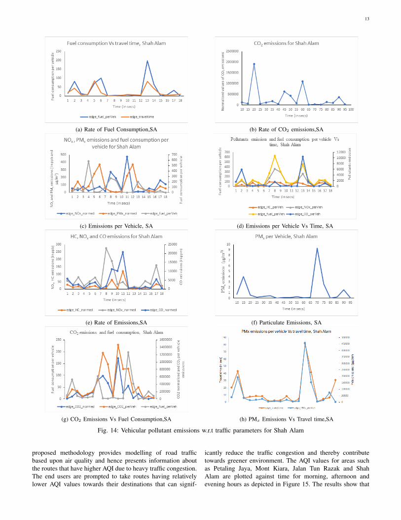
The vehicular emission factor is experimented with regardsto various traffic parameters on simulation platforms and theresults for all the case study areas of Greater KL are plottedas depicted in Figures 11, 12, 13 and 14 respectively. Theresults show that CO2 emission values is the highest during

9

(a) Inst. throughput,Petaling Jaya (b) Inst. delay,Petaling Jaya

(c) Inst. throughput,Mont Kiara (d) Inst. delay,Mont Kiara

(e) Inst. throughput,Shah Alam (f) Inst. delay,Shah Alam

(g) Inst. throughput,Jalan Tun Razak (h) Inst. delay,Jalan Tun Razak

Fig. 10: Traffic flow modelling

10

(a) Rate of Fuel Consumption,PJ (b) Rate of CO2 emissions,PJ

(c) Emissions per Vehicle, PJ (d) Emissions per Vehicle Vs Time, PJ

(e) Rate of Emissions,PJ (f) Particulate Emissions, PJ

(g) CO2 Emissions Vs Fuel Consumption,PJ (h) PMx Emissions Vs Travel time,PJ

Fig. 11: Vehicular pollutant emissions w.r.t traffic parameters for Petaling Jaya

peak hours. The duration of 100 seconds of a simulation run isdivided into frequency intervals of peak and non-peak hours.It can be noted that during peak hours there is considerableamount of CO2 emissions, this might be due to the heavydensity of vehicles moving to and from work places or

home. Other factors affecting the vehicular density irrespectiveof traffic hours are accidents, weather conditions, vehiclesexiting or entering a state/place due to holidays, festivals andso on. The results also interpret that more the travel timeand waiting time of vehicles at junctions and traffic signals,

11

(a) Rate of Fuel Consumption,MK (b) Rate of CO2 emissions,MK

(c) Emissions per Vehicle, MK (d) Emissions per Vehicle Vs Time, MK

(e) Rate of Emissions,MK (f) Particulate Emissions, MK

(g) CO2 Emissions Vs Fuel Consumption,MK (h) PMx Emissions Vs Travel time,MK

Fig. 12: Vehicular pollutant emissions w.r.t traffic parameters for Mont Kiara

higher is the fuel consumption. The emissions from particulatematter (PMx) measured in (µg/m3) for each vehicle also hassignificant effect of harmful emissions into the atmosphereirrespective of the traffic hours, followed by emissions due to

hydrocarbons (HC), NOx and CO. It also indicates that thehigher the fuel consumption, higher is the vehicular emissionsdue to the air pollutants. The rate of vehicular emissions alsodepends upon the factors such as vehicle engine, engine age,

12

(a) Rate of Fuel Consumption,JTR (b) Rate of CO2 emissions,JTR

(c) Emissions per Vehicle, JTR (d) Emissions per Vehicle Vs Time, JTR

(e) Rate of Emissions,JTR (f) Particulate Emissions, JTR

(g) CO2 Emissions Vs Fuel Consumption,JTR (h) PMx Emissions Vs Travel time,JTR

Fig. 13: Vehicular pollutant emissions w.r.t traffic parameters for Jalan Tun Razak

quality of fuel used, year of manufacture for both vehicle andengine, size of engine, exhaust control device and mileageof vehicle per hour. Thus, modelling the vehicular emissionsaccording to fuel and engine parameters can considerablymitigate the traffic induced air pollution and thereby prevent

traffic congestion.

C. Results of Air Quality modelling

The The AQI is calculated based upon the emissions ofair pollutants and vehicular density at a given period. The

13

(a) Rate of Fuel Consumption,SA (b) Rate of CO2 emissions,SA

(c) Emissions per Vehicle, SA (d) Emissions per Vehicle Vs Time, SA

(e) Rate of Emissions,SA (f) Particulate Emissions, SA

(g) CO2 Emissions Vs Fuel Consumption,SA (h) PMx Emissions Vs Travel time,SA

Fig. 14: Vehicular pollutant emissions w.r.t traffic parameters for Shah Alam

proposed methodology provides modelling of road trafficbased upon air quality and hence presents information aboutthe routes that have higher AQI due to heavy traffic congestion.The end users are prompted to take routes having relativelylower AQI values towards their destinations that can signif-

icantly reduce the traffic congestion and thereby contributetowards greener environment. The AQI values for areas suchas Petaling Jaya, Mont Kiara, Jalan Tun Razak and ShahAlam are plotted against time for morning, afternoon andevening hours as depicted in Figure 15. The results show that

14

(a) Air Quality Index, PJ (b) Air Quality Index, JTR

(c) Air Quality Index, MK (d) Air Quality Index, SA

Fig. 15: Air Quality Index w.r.t peak and non-peak hours

AQI is higher during peak hours. Therefore, modelling thetraffic based upon AQI can significantly reduce the congestionoccurring during peak hours.

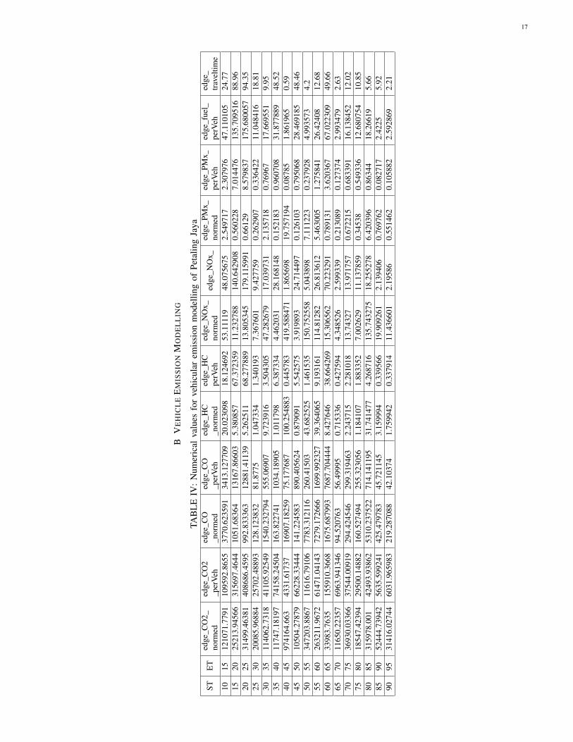
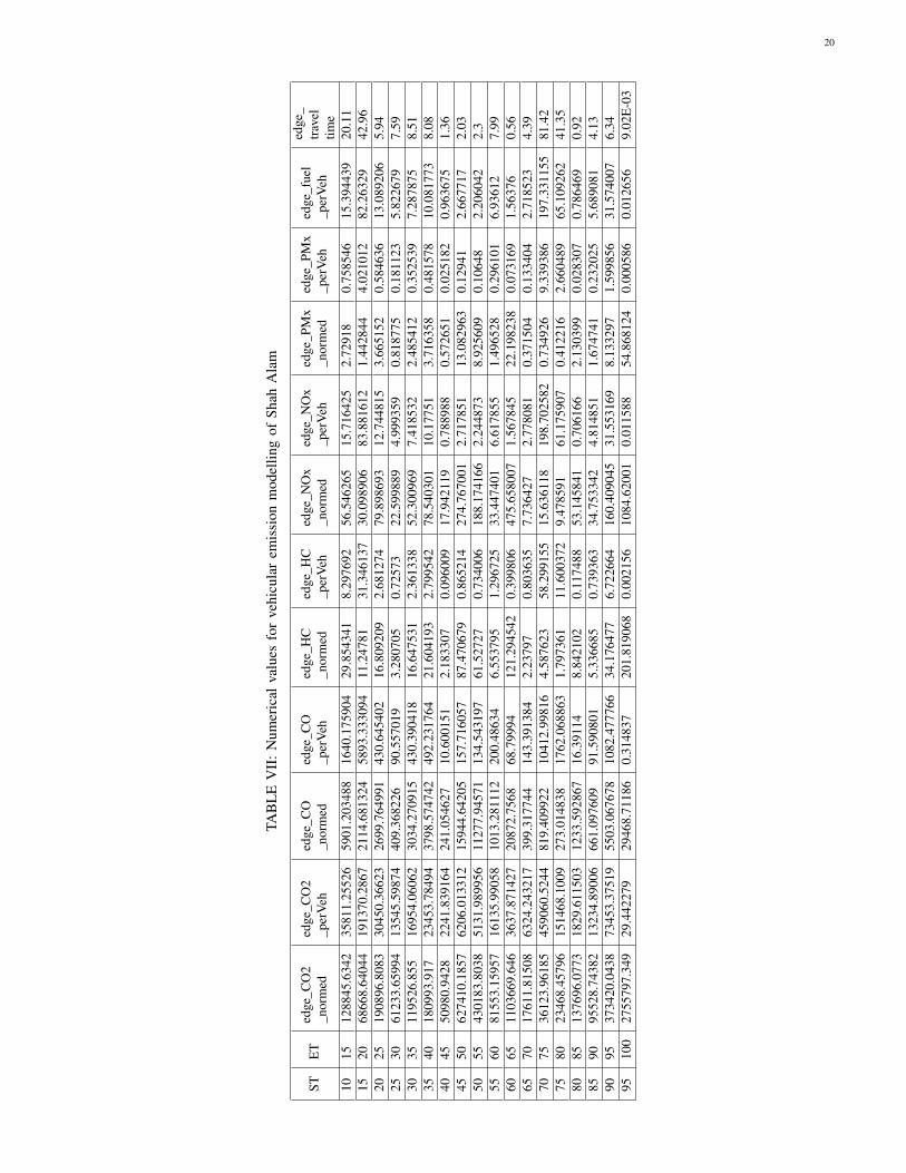
D. Comparative AnalysisAs discussed in previous sections, the traffic congestion can

be mitigated based upon traffic flow/use, vehicular emissionand air quality. The cumulative results are depicted Figures16, 17 and 18 respectively. The numerical values that areobtained after simulations and calculations using formulasare tabulated in Appendix A, B and C respectively. Thesethree factors are dependent on each other and hence havemajor contribution towards modelling and governing trafficcongestion in urban cities. The case study areas consideredin this research belongs to Greater KL according to thedemographical information tabulated in Table II. The higherlevels of air pollution in such areas can cause increased UHIat the surrounding areas as well. The other areas vary foreach parameter depending upon the traffic hours. The resultsshow increase in the pollutant emission with increasing fuelconsumption per vehicle and travel time thereby showing highdependency upon the peak and non-peak hours of the day.Urban areas are the major contributors towards increased AQI,therefore, on a comparative basis, to make Malaysia pollutionfree and to outsmart the traffic congestion, it is necessaryto consider the urban areas and hence balance the levelsof air quality. These areas also contribute towards increasedUHI effects to the surrounding places due to heat generatedfrom vehicle congestion. Hence, the modelling of traffic flowbased upon vehicular emissions and air quality index can bea promising solution towards mitigation of traffic congestion[41]. The current work carried out by the authors of thisresearch is to provide user-based solutions for notifications and

(a) Instantaneous throughput, Greater KL

(b) Instantaneous delay, Greater KL

Fig. 16: Air Quality Index w.r.t peak and non-peak hours,Greater KL

timely updates about the AQI levels different from the existingsolutions [42] and [43] which focus on only traffic flowestimation and environmental impacts. This is implementedthrough integration of obtained AQI values with a real timemobile application for prompting the users with informationof minimal traffic congestion and lesser AQI en route to their

15

(a) CO2 Emissions, Greater KL

(b) Pollutant Emissions, Greater KL

(c) Fuel consumption per vehicle, Greater KL

Fig. 17: Cumulative vehicular Emissions and fuel Consump-tion

destination. The quantitative results show that the pollutionof an urban city not only depends upon the traffic but alsolargely upon other factors such as air quality and vehicularcongestion. The heat generated from vehicles largely affectsthe environmental conditions and causes imbalances in theatmosphere. Needlessly, it can be inferred from the abovesections that air quality imbalance and traffic use form a causeand effect relation.Therefore, mitigation of traffic congestionin such urban areas needs to be addressed to avoid the adverseimpacts of air pollution of urban cities to the country ofMalaysia and on the longer run to prevent health hazardscaused due to traffic induced air pollution. The comparativeresults plotted in Figures 16, 17 and 18 show that in GreaterKL, Jalan Tun Razak has higher instantaneous delay, pollutantemission and fuel consumption per vehicle leading to highervalues of AQI.

Fig. 18: The Air Quality Index w.r.t peak and non-peakhours,Greater KL

V. CONCLUSION AND FUTURE WORK

The relationship between traffic flow, emission of pollutantsand their dispersion into the atmosphere determines the airquality level and provides a wider scope to design trafficmanagement strategies for urban road networks. The proposedproject has revealed that modelling of road traffic flow caneventually reduce the air pollution level. It can be perceivedthat when emission and traffic flow model are combined,the emission rate are better estimated for maintaining the airquality in urban transportation. The implementation of theproposed model via simulation has found that air quality ishighly dependent on the flow of traffic, density of vehicles,waiting time of vehicles at the junctions/intersections, typeof air pollutant, traffic flow rate, fuel consumption rate andacceleration speed. The experimental results provide a widerscope for making the atmosphere free from harmful air pollu-tants and alleviate the traffic congestion causes. The proposedvehicle routing mechanism shows that around 75% of harmfulemission can be reduced by avoiding the traffic congestioncaused by dense traffic and efficient routing of the vehiclesin the path where there is lesser traffic congestion and lowerlevels of emission from harmful air pollutants.The authors currently are focusing upon developing a userfriendly mobile application for timely updates on the AQIvalues and traffic routing from current location towards thedestination in minimal time possible. Future work will includerecording of the AQI values using deployment of an airquality sensor-based instrument near the traffic signals. Thevalues obtained from such real-time measurements are thencompared with existing AQI recording strategies employed bygovernment agencies based on quantitative/statistical analysisfor validation and providing the scope for governing the trafficregulation policies in Malaysia.

16

AP

PE

ND

IXA

TR

AFF

ICF

LO

WM

OD

EL

LIN

G

TAB

LE

III:

Num

eric

alva

lues

oftr

affic

flow

mod

ellin

gfo

rar

eas

belo

ngin

gto

Gre

ater

K.L

Thr

ough

put

Del

ayT

hrou

ghpu

tD

elay

Thr

ough

put

Del

ayT

hrou

ghpu

tD

elay

Tim

eSh

ahA

lam

Peta

ling

jaya

Jala

nTu

nR

azak

Mon

tK

iara

100

19.0

733

00

010

001

00

150.

0020

0002

3000

0.02

3000

0.19

9986

3000

0.00

230

0020

0.02

490

000.

0480

000.

5335

890

000.

7979

1190

0025

0.42

611

000

0.06

412

000

011

495

0.80

2081

9000

300.

952

2000

00.

0817

000

0.02

0266

490

000.

1333

7521

000

350.

522

2200

00.

746

2400

00.

4521

816

000

0.03

4666

921

000

400.

134

3000

00.

045

2900

00.

5214

621

000

0.28

8112

2500

045

0.23

635

000

0.07

229

500

031

005

0.39

971

3300

050

0.52

833

000

0.24

3400

00.

6724

2100

00

3200

055

0.10

2741

000

0.05

0636

000

0.22

8591

4500

00.

2742

8642

000

17

BV

EH

ICL

EE

MIS

SIO

NM

OD

EL

LIN

G

TAB

LE

IV:

Num

eric

alva

lues

for

vehi

cula

rem

issi

onm

odel

ling

ofPe

talin

gJa

ya

STE

Ted

geC

O2

norm

eded

geC

O2

perV

ehed

geC

Ono

rmed

edge

CO

perV

ehed

geH

Cno

rmed

edge

HC

perV

ehed

geN

Ox

norm

eded

geN

Ox

edge

PMx

norm

eded

gePM

xpe

rVeh

edge

fuel

perV

ehed

getr

avel

time

1015

1210

71.7

791

1095

92.8

655

3770

.623

591

3413

.127

709

20.0

2309

818

.124

692

53.1

1119

48.0

7567

52.

5497

172.

3079

7647

.110

105

24.7

715

2025

213.

9456

631

5697

.464

410

51.6

8364

1316

7.86

603

5.38

0857

67.3

7235

911

.232

788

140.

6429

080.

5602

287.

0144

7613

5.70

9516

88.9

620

2531

499.

4638

140

8686

.459

599

2.83

3363

1288

1.41

139

5.26

2511

68.2

7788

913

.805

345

179.

1159

910.

6612

98.

5798

3717

5.68

0057

94.3

525

3020

085.

9688

425

702.

4889

312

8.12

3832

81.8

775

1.04

7334

1.34

0193

7.36

7601

9.42

7759

0.26

2907

0.33

6422

11.0

4841

618

.81

3035

1140

62.7

318

4110

5.92

549

1540

.232

794

555.

0690

79.

7239

163.

5043

0547

.282

679

17.0

3973

12.

1357

180.

7696

717

.669

551

9.95

3540

1174

7.18

197

7415

8.24

504

163.

8227

4110

34.1

8905

1.01

1798

6.38

7334

4.46

2031

28.1

6814

80.

1521

830.

9607

0831

.877

889

48.5

240

4597

4164

.663

4331

.617

3716

907.

1825

975

.177

687

100.

2548

830.

4457

8341

9.58

8471

1.86

5698

19.7

5719

40.

0878

51.

8619

650.

5945

5010

504.

2787

966

228.

3344

414

1.22

4583

890.

4056

240.

8790

915.

5425

753.

9198

9324

.714

497

0.12

6103

0.79

5068

28.4

6918

548

.46

5055

3472

03.8

867

1161

6.79

106

7783

.312

116

260.

4150

343

.682

525

1.46

1535

150.

7525

585.

0438

987.

1112

230.

2379

284.

9935

734.

255

6026

3211

.967

261

471.

0414

372

79.1

7266

616

99.9

9232

739

.364

065

9.19

3161

114.

8128

226

.813

612

5.46

3005

1.27

5841

26.4

2408

12.6

860

6533

983.

7635

1559

10.3

668

1675

.687

993

7687

.704

444

8.42

7646

38.6

6426

915

.306

562

70.2

2329

10.

7891

313.

6203

6767

.022

309

49.6

665

7011

650.

2235

769

63.9

4134

694

.520

763

56.4

9995

0.71

5336

0.42

7594

4.34

8526

2.59

9339

0.21

3089

0.12

7374

2.99

3479

2.63

7075

3693

0.03

366

3754

4.00

919

294.

4245

4629

9.31

9463

2.24

3715

2.28

1018

13.7

4327

13.9

7175

70.

6722

150.

6833

9116

.138

452

12.0

275

8018

547.

4239

429

500.

1488

216

0.52

7494

255.

3230

561.

1841

071.

8833

527.

0026

2911

.137

859

0.34

538

0.54

9336

12.6

8075

410

.85

8085

3159

78.0

0142

493.

9386

253

10.2

3752

271

4.14

1195

31.7

4147

74.

2687

1613

5.74

3275

18.2

5527

86.

4203

960.

8634

418

.266

195.

6685

9052

444.

7394

256

35.5

9924

142

5.47

9783

45.7

2114

53.

1599

940.

3395

6619

.909

261

2.13

9406

0.76

9762

0.08

2717

2.42

255.

9290

9531

416.

0274

460

31.9

6598

321

9.28

7088

42.1

0374

1.75

9942

0.33

7914

11.4

3660

12.

1958

60.

5514

620.

1058

822.

5928

692.

21

18

TAB

LE

V:

Num

eric

alva

lues

for

vehi

cula

rem

issi

onm

odel

ling

ofM

ont

Kia

ra

STE

Ted

geC

O2

norm

eded

geC

O2

perV

ehed

geC

Ono

rmed

edge

CO

perV

ehed

geH

Cno

rmed

edge

HC

perV

ehed

geN

Ox

norm

eded

geN

Ox

perV

ehed

gePM

xno

rmed

edge

PMx

perV

ehed

gefu

elpe

rVeh

edge

trav

eltim

e10

1515

591.

7618

8021

1.19

518

94.8

9317

488.

1741

170.

7732

243.

9778

225.

6555

429

.094

698

0.19

6131

1.00

8988

34.4

7944

136

.615

2080

17.1

7406

554

83.9

2906

959

.266

565

40.5

3967

60.

4561

130.

3119

923.

0021

332.

0535

270.

1126

750.

0770

722.

3573

064

2025

2515

5.63

231

5415

79.5

778

770.

7470

8716

593.

5356

74.

1031

388

.336

942

11.0

4160

323

7.71

6404

0.53

0953

11.4

3097

223

2.80

5677

119.

4725

3039

311.

6335

622

7965

.654

857

2.57

4686

3320

.324

074

3.54

1736

20.5

3830

116

.449

564

95.3

8997

0.75

0174

4.35

0209

97.9

9202

41.2

630

3513

684.

1191

370

388.

3367

810

5.89

2455

544.

6893

390.

7974

814.

1020

795.

1519

3726

.500

520.

1955

231.

0057

330

.256

913

36.5

935

4010

903.

9040

570

2699

.346

445

6.21

5137

2940

0.66

943

2.33

3162

150.

3600

194.

8516

1731

2.66

1255

0.24

1301

15.5

5055

430

2.07

0979

200.

4640

4511

681.

1202

328

624.

5953

168

.916

827

168.

8807

450.

5638

761.

3817

794.

2114

7610

.320

224

0.14

3644

0.35

2001

12.3

0452

415

.44

4550

4950

.722

074

5117

7.52

628

28.6

1267

829

5.78

0304

0.24

2882

2.51

0761

1.79

1287

18.5

1723

0.06

169

0.63

7715

21.9

9908

527

.74

5055

1400

7.47

488

7685

1.51

974

95.6

1690

652

4.59

8803

0.75

8172

4.15

9685

5.18

1404

28.4

2758

90.

1886

721.

0351

4233

.035

205

37.8

5560

3951

3.56

069

2094

0.00

045

313.

2285

216

5.99

3781

2.33

7156

1.23

8563

14.9

3167

37.

9129

60.

5715

080.

3028

689.

0012

0111

.75

6065

8849

6.36

716

5716

.121

797

598.

0773

3938

.630

771

4.71

9137

0.30

4817

32.6

2608

12.

1073

711.

1788

040.

0761

412.

4571

193.

8165

7034

370.

7698

718

5867

.276

348

4.50

286

2620

.052

658

3.02

5273

16.3

5981

114

.354

412

77.6

2454

70.

6555

033.

5447

7379

.895

795

39.3

270

7536

29.1

7544

428

789.

0468

530

.056

957

238.

4318

880.

2215

531.

7575

061.

3824

7610

.966

721

0.05

3878

0.42

7393

12.3

7515

854

.65

7580

1703

0.71

885

1385

00.8

784

432.

4939

4335

17.2

2036

12.

3728

0919

.296

664

7.45

4596

60.6

2387

0.35

4545

2.88

3308

59.5

3600

163

.79

8085

2811

9.93

476

5432

3.45

668

230.

1401

1244

4.59

5853

1.70

0949

3.28

5977

10.6

8067

120

.633

439

0.41

2965

0.79

7785

23.3

5129

822

.44

8590

2811

3.06

145

7199

5.08

393

190.

5604

4448

8.00

8579

1.50

082

3.84

3467

10.3

6617

926

.546

874

0.37

4588

0.95

9286

30.9

4763

736

.52

9095

1844

9.08

7535

595.

7463

111

8.06

3145

227.

7915

240.

9580

11.

8483

886.

7604

0113

.043

546

0.24

0588

0.46

4192

15.3

0111

122

.41

9510

064

09.6

4360

428

7691

.925

166

.501

5729

84.8

7185

30.

4621

4320

.742

941

2.40

6887

108.

0312

860.

1283

385.

7603

612

3.66

5642

80.5

1

19

TAB

LE

VI:

Num

eric

alva

lues

for

vehi

cula

rem

issi

onm

odel

ling

ofJa

lan

Tun

Raz

ak

STE

Ted

geC

O2

norm

eded

geC

O2

perV

ehed

geC

Ono

rmed

edge

CO

perV

ehed

geH

Cno

rmed

edge

HC

perV

ehed

geN

Ox

norm

eded

geN

Ox

perV

ehed

gePM

xno

rmed

edge

PMx

perV

ehed

gefu

elpe

rVeh

edge trav

eltim

e10

1516

8237

.965

860

877.

1708

310

8.45

1782

2202

.753

941

31.6

7194

711

.460

544

74.2

5263

826

.868

433

3.61

2725

1.30

727

26.1

6917

115

.59

1520

2157

18.7

985

2065

5.83

243

424.

6300

4944

2.82

4566

26.1

7119

12.

5059

8393

.182

244

8.92

2527

4.34

569

0.41

6115

8.87

9072

7.11

2025

4345

.397

125

1274

734.

974

214.

0014

6462

777.

9561

41.

0764

9431

5.79

2552

1.95

9223

574.

7437

780.

1012

4529

.700

649

547.

9792

6540

2.66

2530

2252

51.1

599

7271

6.07

278

6154

.775

523

1986

.898

114

33.3

5079

410

.766

376

98.2

6174

431

.721

071

4.67

9668

1.51

0701

31.2

5787

214

.76

3035

1353

9.48

184

5530

9.33

455

73.3

6495

929

9.69

8844

0.64

0552

2.61

6681

4.86

1673

19.8

6013

30.

1641

230.

6704

5123

.775

191

32.6

235

4020

224.

7055

720

5084

.44

416.

6817

6742

25.2

752

2.37

8233

24.1

1597

58.

7769

9689

.001

312

0.41

296

4.18

7532

88.1

5692

632

.340

4534

461.

6701

443

916.

9976

226

4.70

7981

337.

3365

172.

0477

112.

6095

4712

.745

6716

.242

729

0.62

0983

0.79

1364

18.8

7791

514

.39

4550

1637

92.0

467

2276

0.78

231

4200

.147

981

583.

6587

0523

.004

968

3.19

6804

71.7

2486

19.

9669

923.

4138

380.

4743

929.

7839

567.

7550

5510

674.

2528

444

858.

5229

174

.347

744

312.

4462

230.

5820

252.

4459

593.

9548

716

.620

332

0.14

454

0.60

7429

19.2

8277

233

.56

5560

1078

24.7

779

3417

4.01

843

2736

.951

786

867.

4503

4415

.016

414

4.75

9307

47.1

7586

914

.951

935

2.24

1427

0.71

0399

14.6

9004

811

.57

6065

7338

7.00

208

2272

7.14

963

920.

8783

4528

5.18

5923

5.91

8353

1.83

2849

30.1

1849

79.

3273

681.

3485

070.

4176

189.

7693

569.

4665

7020

5349

.255

414

732.

2944

352

53.5

8591

437

6.90

6039

28.7

812

2.06

4839

89.7

4855

66.

4387

974.

2526

950.

3050

996.

3328

35.

7570

7518

3028

.384

631

222.

5102

925

18.5

6248

542

9.63

7421

15.8

3064

32.

7005

2376

.247

983

13.0

0701

83.

4763

680.

5930

2813

.421

118

6.86

7580

4760

.316

713

274.

1158

1354

.011

057

3.11

0147

0.35

8844

0.02

0664

1.92

1476

0.11

0645

0.08

4093

0.00

4842

0.11

783

4.07

8085

2682

2.42

588

3393

.019

319

228.

9303

2228

.959

536

1.69

8783

0.21

4895

10.1

0207

41.

2779

060.

4976

530.

0629

531.

4585

034.

8485

9040

30.0

7869

2565

0.51

627

.936

2817

7.80

7939

0.21

3122

1.35

647

1.48

281

9.43

7739

0.05

3299

0.33

9239

11.0

2607

215

.33

9095

3158

74.1

149

3971

9.67

845

7320

.977

7392

0.57

8381

40.8

1523

5.13

2322

136.

7247

417

.192

496.

4093

580.

8059

4617

.073

867

8.05

9510

028

187.

0360

134

240.

2801

117

2.60

5485

209.

6729

911.

4244

071.

7303

0210

.265

782

12.4

7038

70.

3596

860.

4369

314

.718

461

17.7

9

20

TAB

LE

VII

:N

umer

ical

valu

esfo

rve

hicu

lar

emis

sion

mod

ellin

gof

Shah

Ala

m

STE

Ted

geC

O2

norm

eded

geC

O2

perV

ehed

geC

Ono

rmed

edge

CO

perV

ehed

geH

Cno

rmed

edge

HC

perV

ehed

geN

Ox

norm

eded

geN

Ox

perV

ehed

gePM

xno

rmed

edge

PMx

perV

ehed

gefu

elpe

rVeh

edge

trav

eltim

e10

1512

8845

.634

235

811.

2552

659

01.2

0348

816

40.1

7590

429

.854

341

8.29

7692

56.5

4626

515

.716

425

2.72

918

0.75

8546

15.3

9443

920

.11

1520

6866

8.64

044

1913

70.2

867

2114

.681

324

5893

.333

094

11.2

4781

31.3

4613

730

.098

906

83.8

8161

21.

4428

444.

0210

1282

.263

2942

.96

2025

1908

96.8

083

3045

0.36

623

2699

.764

991

430.

6454

0216

.809

209

2.68

1274

79.8

9869

312

.744

815

3.66

5152

0.58

4636

13.0

8920

65.

9425

3061

233.

6599

413

545.

5987

440

9.36

8226

90.5

5701

93.

2807

050.

7257

322

.599

889

4.99

9359

0.81

8775

0.18

1123

5.82

2679

7.59

3035

1195

26.8

5516

954.

0606

230

34.2

7091

543

0.39

0418

16.6

4753

12.

3613

3852

.300

969

7.41

8532

2.48

5412

0.35

2539

7.28

7875

8.51

3540

1809

93.9

1723

453.

7849

437

98.5

7474

249

2.23

1764

21.6

0419

32.

7995

4278

.540

301

10.1

7751

3.71

6358

0.48

1578

10.0

8177

38.

0840

4550

980.

9428

2241

.839

164

241.

0546

2710

.600

151

2.18

3307

0.09

6009

17.9

4211

90.

7889

880.

5726

510.

0251

820.

9636

751.

3645

5062

7410

.185

762

06.0

1331

215

944.

6420

515

7.71

6057

87.4

7067

90.

8652

1427

4.76

7001

2.71

7851

13.0

8296

30.

1294

12.

6677

172.

0350

5543

0183

.803

851

31.9

8995

611

277.

9457

113

4.54

3197

61.5

2727

0.73

4006

188.

1741

662.

2448

738.

9256

090.

1064

82.

2060

422.

355

6081

553.

1595

716

135.

9905

810

13.2

8111

220

0.48

634

6.55

3795

1.29

6725

33.4

4740

16.

6178

551.

4965

280.

2961

016.

9361

27.

9960

6511

0366

9.64

636

37.8

7142

720

872.

7568

68.7

9994

121.

2945

420.

3998

0647

5.65

8007

1.56

7845

22.1

9823

80.

0731

691.

5637

60.

5665

7017

611.

8150

863

24.2

4321

739

9.31

7744

143.

3913

842.

2379

70.

8036

357.

7364

272.

7780

810.

3715

040.

1334

042.

7185

234.

3970

7536

123.

9618

545

9060

.524

481

9.40

9922

1041

2.99

816

4.58

7623

58.2

9915

515

.636

118

198.

7025

820.

7349

269.

3393

8619

7.33

1155

81.4

275

8023

468.

4579

615

1468

.100

927

3.01

4838

1762

.068

863

1.79

7361

11.6

0037

29.

4785

9161

.175

907

0.41

2216

2.66

0489

65.1

0926

241

.35

8085

1376

96.0

773

1829

.611

503

1233

.592

867

16.3

9114

8.84

2102

0.11

7488

53.1

4584

10.

7061

662.

1303

990.

0283

070.

7864

690.

9285

9095

528.

7438

213

234.

8900

666

1.09

7609

91.5

9080

15.

3366

850.

7393

6334

.753

342

4.81

4851

1.67

4741

0.23

2025

5.68

9081

4.13

9095

3734

20.0

438

7345

3.37

519

5503

.067

678

1082

.477

766

34.1

7647

76.

7226

6416

0.40

9045

31.5

5316

98.

1332

971.

5998

5631

.574

007

6.34

9510

027

5579

7.34

929

.442

279

2946

8.71

186

0.31

4837

201.

8190

680.

0021

5610

84.6

2001

0.01

1588

54.8

6812

40.

0005

860.

0126

569.

02E

-03

21

CA

IRQ

UA

LIT

YM

OD

EL

LIN

G

TAB

LE

VII

I:A

irQ

ualit

yM

odel

ling

num

eric

alva

lues

for

area

sbe

long

ing

toG

reat

erK

.L

Stat

eL

ocat

ion

8am

9am

10am

11am

12pm

13(1

pm)

14(2

pm)

15(3

pm)

16(4

pm)

17(5

pm)

18(6

pm)

19(7

pm)

20(8

pm)

W.P

.K

UA

LA

LU

MPU

RM

ont

Kia

ra39

4045

5233

3335

3538

4852

5149

W.P

.K

UA

LA

LU

MPU

RJa

lan

Tun

Raz

ak33

3844

4934

3434

3945

4950

4945

SEL

AN

GO

RPe

talin

gJa

ya39

3942

4335

3635

3438

4241

4040

SEL

AN

GO

RSh

ahA

lam

4748

4645

3836

3736

3942

4445

48

22

ACKNOWLEDGMENT

This research is supported by Grand Challenge GrantUM.0000007/HRU.GC.SS (GC002B-15SUS) from Sustain-able Science Cluster, the Faculty program grant GPF009D-2018, University of Malaya and UMRG project RP036A-15AET.The authors would like to thank the University of Malaya Post-Doctoral Research Fellowship scheme for the required supportprovided to carry out this research. We would also like toextend our thankful regards to the anonymous reviewers forproviding constructive suggestions that aided in improvisationof this manuscript.

REFERENCES

[1] S. Wang, S. Djahel, Z. Zhang, and J. McManis, “Next road rerouting: Amultiagent system for mitigating unexpected urban traffic congestion,”IEEE Transactions on Intelligent Transportation Systems, vol. 17, no. 10,pp. 2888–2899, 2016.

[2] G. M. Grossman and A. B. Krueger, “Economic growth and theenvironment,” The quarterly journal of economics, vol. 110, no. 2, pp.353–377, 1995.

[3] S. Wang, S. Djahel, and J. McManis, “An adaptive and vanets-basednext road re-routing system for unexpected urban traffic congestionavoidance,” in 2015 IEEE vehicular networking conference (VNC).IEEE, 2015, pp. 196–203.

[4] R. Doolan and G.-M. Muntean, “Vanet-enabled eco-friendly roadcharacteristics-aware routing for vehicular traffic,” in 2013 IEEE 77thVehicular Technology Conference (VTC Spring). IEEE, 2013, pp. 1–5.

[5] L. Y. Siew, L. Y. Chin, and P. M. J. Wee, “Arima and integratedarfima models for forecasting air pollution index in shah alam, selangor,”Malaysian Journal of Analytical Sciences, vol. 12, no. 1, pp. 257–263,2008.

[6] T. Wong, W. Tam, I. Yu, A. Wong, A. Lau, S. Ng, D. Yeung, andC. Wong, “A study of the air pollution index reporting system,” FinalReport, Tender Ref. AP, pp. 07–085, 2012.

[7] G. Wang, F. Van den Bosch, and M. Kuffer, “Modelling urban trafficair pollution dispersion.” ITC, 2008.

[8] D. J. S. . R. Blewitt, “Traffic modelling guidelines,” in TfL TrafficManager and Network Performance Best Practice, 2010.

[9] A. Hickman and D. Colwill, “The estimation of air pollution concentra-tions from road traffic,” Tech. Rep., 1982.

[10] M. A. Association, “Malaysian automotive association market review2017,” 2017.

[11] S. Pandian, S. Gokhale, and A. K. Ghoshal, “Evaluating effects of trafficand vehicle characteristics on vehicular emissions near traffic intersec-tions,” Transportation Research Part D: Transport and Environment,vol. 14, no. 3, pp. 180–196, 2009.

[12] L. Xia and Y. Shao, “Modelling of traffic flow and air pollution emissionwith application to hong kong island,” Environmental Modelling &Software, vol. 20, no. 9, pp. 1175–1188, 2005.

[13] K. K. Khedo, R. Perseedoss, A. Mungur et al., “A wireless sensor net-work air pollution monitoring system,” arXiv preprint arXiv:1005.1737,2010.

[14] J.-H. Liu, Y.-F. Chen, T.-S. Lin, D.-W. Lai, T.-H. Wen, C.-H. Sun, J.-Y.Juang, and J.-A. Jiang, “Developed urban air quality monitoring systembased on wireless sensor networks,” in Sensing technology (icst), 2011fifth international conference on. IEEE, 2011, pp. 549–554.

[15] R. S. Andy Ford and G. Bell, “Traffic modelling report,” in TechnicalReport 34 Traffic Modelling Report, 2012.

[16] J. Smith, R. Blewitt et al., “Traffic modelling guidelines,” Trafficmanager and network performance best practice. Version, vol. 3, 2010.

[17] D. A. Chu, Y. Kaufman, G. Zibordi, J. Chern, J. Mao, C. Li, andB. Holben, “Global monitoring of air pollution over land from the earthobserving system-terra moderate resolution imaging spectroradiometer(modis),” Journal of Geophysical Research: Atmospheres, vol. 108, no.D21, 2003.

[18] R. M. E. S. Nick Benbow, Ian Wilkinson and D. Carter, “Transportfor south hampshire evidence base road traffic model calibration andvalidation,” in Summary Report 4 Report for Transport for SouthHampshire, 2011.

[19] N. H. A. Rahman, M. H. Lee, M. T. Latif et al., “Forecasting ofair pollution index with artificial neural network,” Jurnal Teknologi(Sciences and Engineering), vol. 63, no. 2, pp. 59–64, 2013.

[20] J. Kwon, G. Ahn, G. Kim, J. C. Kim, and H. Kim, “A study on ndir-based co2 sensor to apply remote air quality monitoring system,” inICCAS-SICE, 2009. IEEE, 2009, pp. 1683–1687.

[21] N. Kularatna and B. Sudantha, “An environmental air pollution monitor-ing system based on the ieee 1451 standard for low cost requirements,”IEEE Sensors Journal, vol. 8, no. 4, pp. 415–422, 2008.

[22] O. A. Postolache, J. D. Pereira, and P. S. Girao, “Smart sensorsnetwork for air quality monitoring applications,” IEEE Transactions onInstrumentation and Measurement, vol. 58, no. 9, pp. 3253–3262, 2009.

[23] J. Zambrano-Martinez, C. Calafate, D. Soler, J.-C. Cano, and P. Man-zoni, “Modeling and characterization of traffic flows in urban environ-ments,” Sensors, vol. 18, no. 7, p. 2020, 2018.

[24] V. Astarita, V. P. Giofre, G. Guido, and A. Vitale, “A single intersectioncooperative-competitive paradigm in real time traffic signal settingsbased on floating car data,” Energies, vol. 12, no. 3, p. 409, 2019.

[25] J. Wang, N. Cao, and G. Yao, “Research on model of feasible timing oftraffic light for intersection control,” in 2018 International Conference onMechanical, Electronic, Control and Automation Engineering (MECAE2018). Atlantis Press, 2018.

[26] S. Kaufmann, B. S. Kerner, H. Rehborn, M. Koller, and S. L. Klenov,“Aerial observations of moving synchronized flow patterns in over-saturated city traffic,” Transportation research part C: emerging tech-nologies, vol. 86, pp. 393–406, 2018.

[27] T. Nagatani, G. Ichinose, and K.-i. Tainaka, “Traffic jams induce dy-namical phase transition in spatial rock–paper–scissors game,” PhysicaA: Statistical Mechanics and its Applications, vol. 492, pp. 1081–1087,2018.

[28] A. I. Delis, I. K. Nikolos, and M. Papageorgiou, “A macroscopic multi-lane traffic flow model for acc/cacc traffic dynamics,” TransportationResearch Record, vol. 2672, no. 20, pp. 178–192, 2018.

[29] J. Aguilar, D. Monaenkova, V. Linevich, W. Savoie, B. Dutta, H.-S.Kuan, M. Betterton, M. Goodisman, and D. Goldman, “Collective clogcontrol: Optimizing traffic flow in confined biological and robophysicalexcavation,” Science, vol. 361, no. 6403, pp. 672–677, 2018.

[30] M. Akbarzadeh and E. Estrada, “Communicability geometry capturestraffic flows in cities,” Nature Human Behaviour, vol. 2, no. 9, p. 645,2018.

[31] I. Klein, N. Levy, and E. Ben-Elia, “An agent-based model of the emer-gence of cooperation and a fair and stable system optimum using atison a simple road network,” Transportation research part C: emergingtechnologies, vol. 86, pp. 183–201, 2018.

[32] A. Olia, S. Razavi, B. Abdulhai, and H. Abdelgawad, “Traffic capacityimplications of automated vehicles mixed with regular vehicles,” Journalof Intelligent Transportation Systems, vol. 22, no. 3, pp. 244–262, 2018.

[33] S. Fulari, A. Thankappan, L. Vanajakshi, and S. Subramanian, “Trafficflow estimation at error prone locations using dynamic traffic flowmodeling,” Transportation letters, vol. 11, no. 1, pp. 43–53, 2019.

[34] S. Chen, X. Wei, N. Xia, Z. Yan, Y. Yuan, H. M. Zhang, M. Li,and L. Cheng, “Understanding road performance using online trafficcondition data,” Journal of Transport Geography, vol. 74, pp. 382–394,2019.

[35] “Air quality index from wikipedia, the free encyclopedia,” https://en.wikipedia.org/wiki/Air quality index, accessed: 2019-03-05.

[36] Y. B. Gaididei, P. L. Christiansen, M. P. Sørensen, and J. J. Rasmussen,“Analytical solutions of pattern formation for a class of discrete aw-rascle-zhang traffic models,” Communications in Nonlinear Science andNumerical Simulation, 2019.

[37] X. Mao, J. Wang, C. Yuan, W. Yu, and J. Gan, “A dynamic trafficassignment model for the sustainability of pavement performance,”Sustainability, vol. 11, no. 1, p. 170, 2019.

[38] B. Sharma and S. Kumar, “Delay optimization using genetic algorithmat the road intersection,” International Journal of Information RetrievalResearch (IJIRR), vol. 9, no. 2, pp. 1–10, 2019.

[39] H. Fu, K. Chen, S. Chen, A. Kouvelas, and N. Geroliminis, “Modelingand integrated control of macroscopic heterogeneous traffic flow in largescale urban network using coloured petri net,” in 2019 TRB AnnualMeeting: Compendium of Papers. The National Academies of Sciences,Engineering, and Medicine, 2019, pp. 19–04 885.

[40] M. Ministry of Transport, “Transport statistics malaysia,” in TransportStatistics Malaysia 2016, 2016.

[41] Y. Gu, X. Cai, D. Han, and D. Z. Wang, “A tri-level optimizationmodel for a private road competition problem with traffic equilibriumconstraints,” European Journal of Operational Research, vol. 273, no. 1,pp. 190–197, 2019.

23

[42] A. Abdalrahman and W. Zhuang, “Pev charging infrastructure sitingbased on spatial-temporal traffic flow distribution,” IEEE Transactionson Smart Grid, 2019.

[43] L. C. Bento, R. Parafita, H. A. Rakha, and U. J. Nunes, “A study ofthe environmental impacts of intelligent automated vehicle control atintersections via v2v and v2i communications,” Journal of IntelligentTransportation Systems, pp. 1–19, 2019.

Shaik Shabana Anjum received the B.Eng. degreein computer science and engineering, the M.Eng.degree (Hons.) in software engineering both fromAnna University, Chennai, India, in 2010 and 2012respectively and the Ph.D. degree in computer sci-ence from the University of Malaya, Malaysia, in2018. She has also served as a Research Assistant forprojects involving traffic congestion and the Internetof Things (IoT) with the University of Malaya. Sheis currently a Post-doctoral Research Fellow withthe Centre for Mobile Cloud Computing Research,

Faculty of Computer Science and Information Technology, University ofMalaya. Her research interests include the IoT, wireless sensor networks, radiofrequency identification, adhoc networks, cognitive radio and energy harvest-ing. She has been accoladed with many awards at international competitionsand also had received appreciation at the faculty level for her projects.

Rafidah Md Noor received the BIT degree fromUniversity Utara Malaysia in 1998, the M.Sc. de-gree in computer science from Universiti TeknologiMalaysia in 2000 and the Ph.D. degree in com-puting from Lancaster University, U.K. in 2010.She is currently an Associate Professor with theDepartment of Computer System and Technology,Faculty of Computer Science and Information Tech-nology, University of Malaya and the Director ofthe Centre of Mobile Cloud Computing Research,which focuses on high impact research. She has

performed nearly RM 665 606.00 for High-Impact Research, Ministry ofEducation Grant and other research grants from the University of Malaya andpublic sectors. She has published more than 50 journals in Science CitationIndex Expanded Non-Science Citation Index, proceeding articles publishedin international/national conferences and a few book chapters. Her researchis related to a field of transportation systems in computer science researchdomain, including vehicular networks, wireless networks, network mobility,quality of service and the Internet of Things.

Nasrin Aghamohammadi is an Associate Profes-sor in the Department of Social and PreventiveMedicine and has a high calibre with extensiveresearch experience in the field of Air PollutionEngineering and Health Impact Assessment. She hasserved as the head of Sustainability Cluster’s GrandChallenge research which comprises of four sub-groups monitoring the incidence of UHI, assessingthe public behaviour towards the UHI phenomenon,modelling the traffic congestion in the city centresas well as evaluating the property value of green

neighbourhood of Greater Kuala Lumpur. She published research articles onvarious fields comprising of environment and public health in total 36 ISI-cited journal articles with h-index of 13.

Ismail Ahmedy received the B.Sc. degree in com-puter science from University Teknologi Malaysia,in 2006, the M.Sc. degree in computer science fromThe University of Queensland, Australia, and thePh.D. degree in wireless networks system specializ-ing in wireless sensor networks in the routing systemfrom Universiti Teknologi Malaysia. He has beenone of the academic members with the Departmentof Computer System and Technology, University ofMalaya since 2007. His research interests includewireless sensor networks, the Internet of Things,

optimization algorithm and energy management. He was a recipient of theFull Scholarship to pursue his master’s degree.

Miss Laiha Mat Kiah joined the Faculty of Com-puter Science and Information Technology, Univer-sity of Malaya, Malaysia as a tutor in 1997. She wasappointed as a lecturer in 2001. She received herBSc. (Hons) in Computer Science from the Univer-sity of Malaya in 1997, a MSc from Royal Holloway,University of London, UK in 1998 and a Ph.D. alsofrom Royal Holloway, University of London in 2007.She is a full Professor at the Department of Com-puter System and Technology, Faculty of ComputerScience and Information Technology, University of

Malaya. Since 2008, she has been actively doing research particularly in theSecurity area of Computing and Networking. Amongst of her research grantswere a High-Impact Research Grant by the Ministry of Higher Education,Malaysia in 2012 for duration of 4 years, working on secure frameworkfor Electronic Medical Records, and a eScience grant by the Ministry ofScience, Technology and Innovation in 2013 for the duration of 3 years,working on Secure Group Communication for Critical National InformationInfrastructure (CNII). Her current research interests include Cyber Security,IoT and Cryptography.

Nornazlita Hussin is a lecturer at Multimedia Unit,under Department of Computer System and Technol-ogy, Faculty of Computer Science and InformationTechnology, University of Malaya. She received aBachelor degree in Computer Science from Univer-sity of Malaya in 1999 and a Master degree in Multi-media Technology from University of Bath in 2000.She teaches multimedia subjects for undergraduatestudents. Her expertise is in the area of AugmentedReality, Virtual Reality and Edutainment.

Mohammad Hossein Anisi received the Ph.D. de-gree from the University of Technology Malaysia,Johor Bahru, Malaysia. He is with the School ofComputer Science and Electronic Engineering, Uni-versity of Essex, Colchester, U.K. He was a Se-nior Lecturer with the Faculty of Computer Scienceand Information Technology, University of Malaya,Kuala Lumpur, Malaysia. He has also collaboratedactively with researchers in several other disciplinesof computer science. He has authored and co-authored several papers in high-quality journals and

conferences. His current research interests include Internet of Things, wirelesssensor networks with their applications, mobile adhoc networks and intelligenttransportation systems. He was also a recipient of the Best PostgraduateStudent Award. He is an Associate Editor of AdHoc and Sensor WirelessNetworks (SCIE) and the KSII Transactions on Internet and InformationSystems (SCIE). He is also an active member of the ACM, the InternationalAssociation of Engineers, and the Institute of Research Engineers and Doctors.

24

Muhammad Ahsan Qureshi received his Ph.D.from University of Malaya, Kuala Lumpur, Malaysiain 2016. His major work is on radio propagationmodelling for Vehicular Ad Hoc Networks. He iscurrently serving as Assistant Professor in the De-partment of Computer Science and Software Engi-neering, International Islamic University, Islamabad,Pakistan. His research interests include WirelessCommunication, Vehicular AdHoc Networks, TrafficManagement and Internet of Vehicles.