modelo bobinas de helmholtz

Solved with COMSOL Multiphysics 5.0

Magne t i c F i e l d o f a He lmho l t z C o i l

Introduction

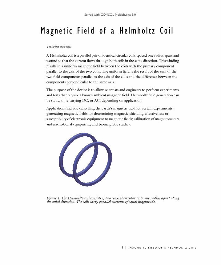
A Helmholtz coil is a parallel pair of identical circular coils spaced one radius apart and wound so that the current flows through both coils in the same direction. This winding results in a uniform magnetic field between the coils with the primary component parallel to the axis of the two coils. The uniform field is the result of the sum of the two field components parallel to the axis of the coils and the difference between the components perpendicular to the same axis.

The purpose of the device is to allow scientists and engineers to perform experiments and tests that require a known ambient magnetic field. Helmholtz field generation can be static, time-varying DC, or AC, depending on application.

Applications include cancelling the earth’s magnetic field for certain experiments; generating magnetic fields for determining magnetic shielding effectiveness or susceptibility of electronic equipment to magnetic fields; calibration of magnetometers and navigational equipment; and biomagnetic studies.

Figure 1: The Helmholtz coil consists of two coaxial circular coils, one radius apart along the axial direction. The coils carry parallel currents of equal magnitude.

1 | M A G N E T I C F I E L D O F A H E L M H O L T Z C O I L


2 | M A G

Model Definition

The model is built using the 3D Magnetic Fields interface. The model geometry is shown in Figure 2.

Figure 2: The model geometry.

D O M A I N E Q U A T I O N S

Assuming static currents and fields, the magnetic vector potential A must satisfy the following equation:

where μ is the permeability, and Je denotes the externally applied current density.

The relations between the magnetic field H, the magnetic flux density B and the potential are given by

This model uses the permeability of vacuum, that is, μ = 4π · 10−7 H/m. The external current density is computed using a homogenized model for the coils, each one made

∇ μ 1– ∇ A×( )× Je=

B ∇ A×=

H μ 1– B=

N E T I C F I E L D O F A H E L M H O L T Z C O I L


by 10 wire turns and excited by a current of 0.25 mA. The currents are specified to be parallel for the two coils.

Results and Discussion

Figure 3 shows the magnetic flux density between the coils. You can see that the flux is relatively uniform between the coils, except for the region close to the edges of the coil.

Figure 3: The slice plot shows the magnetic flux density. The arrows indicate the magnetic field (H) strength and direction.

This uniformity is the main property and often the sought feature of a Helmholtz coil.

Model Library path: ACDC_Module/Inductive_Devices_and_Coils/helmholtz_coil

Modeling Instructions

From the File menu, choose New.



4 | M A G

N E W

1 In the New window, click Model Wizard.

M O D E L W I Z A R D

1 In the Model Wizard window, click 3D.

2 In the Select physics tree, select AC/DC>Magnetic Fields (mf).

3 Click Add.

4 Click Study.

5 In the Select study tree, select Preset Studies>Stationary.

6 Click Done.

D E F I N I T I O N S

Parameters1 On the Model toolbar, click Parameters.

2 In the Settings window for Parameters, locate the Parameters section.

3 In the table, enter the following settings:

G E O M E T R Y 1

On the Geometry toolbar, click Work Plane.

Square 1 (sq1)1 On the Work plane toolbar, click Primitives and choose Square.

2 In the Settings window for Square, locate the Size section.

3 In the Side length text field, type 0.05.

4 Locate the Position section. From the Base list, choose Center.

5 In the xw text field, type -0.4.

6 In the yw text field, type 0.2.

Square 2 (sq2)1 On the Work plane toolbar, click Primitives and choose Square.

2 In the Settings window for Square, locate the Size section.

3 In the Side length text field, type 0.05.

4 Locate the Position section. From the Base list, choose Center.

Name Expression Value Description

I0 0.25[mA] 2.5000E-4 A Coil current



5 In the xw text field, type -0.4.

6 In the yw text field, type -0.2.

Work Plane 1 (wp1)On the Geometry toolbar, click Revolve.

Sphere 1 (sph1)1 On the Geometry toolbar, click Sphere.

2 In the Model Builder window, under Component 1 (comp1)>Geometry 1 right-click Sphere 1 (sph1) and choose Build All Objects.

3 Click the Zoom Extents button on the Graphics toolbar.

Your geometry is now complete. To see its interior, choose wireframe rendering:

4 Click the Wireframe Rendering button on the Graphics toolbar.

A D D M A T E R I A L

1 On the Model toolbar, click Add Material to open the Add Material window.

2 Go to the Add Material window.

3 In the tree, select Built-In>Air.



6 | M A G

4 Click Add to Component in the window toolbar.

By default, the first material you add applies on all domains so you need not alter any settings.

5 On the Model toolbar, click Add Material to close the Add Material window.

M A G N E T I C F I E L D S ( M F )

Multi-Turn Coil 11 On the Physics toolbar, click Domains and choose Multi-Turn Coil.

2 Select Domain 2 only.

3 In the Settings window for Multi-Turn Coil, locate the Coil Type section.

4 From the list, choose Circular.

5 Locate the Multi-Turn Coil section. In the N text field, type 10.

6 In the Icoil text field, type I0.

In order to specify the direction of the wires in the circular coil, you need to add a Reference Edge subfeature and select a group of edges forming a circle. The path of the wires will be automatically computed from the geometry of the selected edges. For the best results, the radius of the circular edges selected should be close to the average radius of the coil.

Reference Edge 11 Right-click Component 1 (comp1)>Magnetic Fields (mf)>Multi-Turn Coil 1 and choose

Edges>Reference Edge.

2 In the Settings window for Reference Edge, locate the Edge Selection section.

3 Click Clear Selection.



4 Select Edges 20, 21, 36, and 39 only.

Now set up the second coil in the same way.

Multi-Turn Coil 21 On the Physics toolbar, click Domains and choose Multi-Turn Coil.

2 Select Domain 3 only.

3 In the Settings window for Multi-Turn Coil, locate the Coil Type section.

4 From the list, choose Circular.

5 Locate the Multi-Turn Coil section. In the N text field, type 10.

6 In the Icoil text field, type I0.

Reference Edge 11 Right-click Component 1 (comp1)>Magnetic Fields (mf)>Multi-Turn Coil 2 and choose

Edges>Reference Edge.

2 In the Settings window for Reference Edge, locate the Edge Selection section.

3 Click Clear Selection.

4 Select Edges 25, 26, 56, and 59 only.



8 | M A G

M E S H 1

1 In the Model Builder window, under Component 1 (comp1) click Mesh 1.

2 In the Settings window for Mesh, locate the Mesh Settings section.

3 From the Element size list, choose Coarse.

Free Tetrahedral 1Right-click Component 1 (comp1)>Mesh 1 and choose Free Tetrahedral.

Size 11 In the Model Builder window, under Component 1 (comp1)>Mesh 1 right-click Free

Tetrahedral 1 and choose Size.

2 In the Settings window for Size, locate the Geometric Entity Selection section.

3 From the Geometric entity level list, choose Domain.

4 Select Domains 2 and 3 only.

5 Locate the Element Size section. Click the Custom button.

6 Locate the Element Size Parameters section. Select the Maximum element size check box.

7 In the associated text field, type 0.05.

8 Click the Build All button.

S T U D Y 1

1 In the Model Builder window, click Study 1.

2 In the Settings window for Study, locate the Study Settings section.

3 Clear the Generate default plots check box.

4 On the Model toolbar, click Compute.

Add a selection to the computed data set to exclude the outer boundaries.

D E F I N I T I O N S

Explicit 11 On the Definitions toolbar, click Explicit.

2 Select Domains 2 and 3 only.

3 In the Settings window for Explicit, locate the Output Entities section.

4 From the Output entities list, choose Adjacent boundaries.

5 Right-click Component 1 (comp1)>Definitions>Explicit 1 and choose Rename.

6 In the Rename Explicit dialog box, type Coils in the New label text field.



7 Click OK.

Now add the plots.

R E S U L T S

In the Model Builder window, expand the Results node.

Data Sets1 On the Results toolbar, click Selection.

2 In the Settings window for Selection, locate the Geometric Entity Selection section.

3 From the Geometric entity level list, choose Boundary.

4 From the Selection list, choose Coils.

3D Plot Group 11 On the Results toolbar, click 3D Plot Group.

2 In the Model Builder window, under Results right-click 3D Plot Group 1 and choose Slice.

3 In the Settings window for Slice, locate the Plane Data section.

4 From the Plane list, choose xy-planes.

5 In the Planes text field, type 1.

6 Click Replace Expression in the upper-right corner of the Expression section. From the menu, choose Model>Component 1>Magnetic Fields>Magnetic>mf.normB -

Magnetic flux density norm.

7 On the 3D plot group toolbar, click Plot.

8 In the Model Builder window, right-click 3D Plot Group 1 and choose Arrow Volume.

9 In the Settings window for Arrow Volume, click Replace Expression in the upper-right corner of the Expression section. From the menu, choose Model>Component

1>Magnetic Fields>Magnetic>mf.Hx,mf.Hy,mf.Hz - Magnetic field.

10 Locate the Arrow Positioning section. Find the x grid points subsection. In the Points text field, type 24.

11 Find the y grid points subsection. In the Points text field, type 10.

12 Find the z grid points subsection. In the Points text field, type 1.

13 Locate the Coloring and Style section. Select the Scale factor check box.

14 In the associated text field, type 25.



10 | M A


To make the coil look like a solid object, you can add a surface plot on its boundaries.

16 Right-click 3D Plot Group 1 and choose Surface.

17 In the Settings window for Surface, locate the Expression section.

18 In the Expression text field, type 1.

19 Locate the Coloring and Style section. From the Coloring list, choose Uniform.

20 From the Color list, choose White.

To verify that the current path is computed correctly, plot the Coil direction variable for each coil.

3D Plot Group 21 On the Model toolbar, click Add Plot Group and choose 3D Plot Group.

2 In the Model Builder window, under Results right-click 3D Plot Group 2 and choose Streamline.

3 Select Boundary 5 only.

4 In the Settings window for Streamline, click Replace Expression in the upper-right corner of the Expression section. From the menu, choose Model>Component

G N E T I C F I E L D O F A H E L M H O L T Z C O I L


1>Magnetic Fields>Coil parameters>mf.mtcd1.eCoilx,...,mf.mtcd1.eCoilz - Coil

direction.

5 In the Model Builder window, right-click 3D Plot Group 2 and choose Streamline.

6 Select Boundary 12 only.

7 In the Settings window for Streamline, click Replace Expression in the upper-right corner of the Expression section. From the menu, choose Model>Component

1>Magnetic Fields>Coil parameters>mf.mtcd2.eCoilx,...,mf.mtcd2.eCoilz - Coil

direction.

8 Locate the Coloring and Style section. From the Color list, choose Blue.




12 | M A
G N E T I C F I E L D O F A H E L M H O L T Z C O I L

modelo bobinas de helmholtz

Documents