models for bonding in chemistry (magnasco/models for bonding in chemistry) || an introduction to...

3An Introduction to Bonding

in Solids

3.1 The Linear Polyene Chain3.1.1 Butadiene N¼4

3.2 The Closed Polyene Chain3.2.1 Benzene N¼6

3.3 A Model for the One-dimensional Crystal3.4 Electronic Bands in Crystals3.5 Insulators, Conductors, Semiconductors and Superconductors3.6 Appendix: the Trigonometric Identity

In the previous chapter, we saw that immediate solution of the N-dimensional (DN) H€uckel secular equation was possible for the firstmembers of the series, ethylene ðN ¼ 2Þ, allyl radical ðN ¼ 3Þ andbutadiene ðN ¼ 4Þ, but for higher values of N only symmetry can helpin finding the solutions, unlesswe have at our disposal the general solutionfor the linear polyene chain of N atoms. The secular equations for linearand closed polyene chains, even with different bs for single and doublebonds, were first solved by Lennard-Jones (1937) and rederived byCoulson (1938). In the following, we present a simple derivation of thegeneral solution for the N-atom linear and closed polyene chains (equalbs) which are useful for introducing the general theory of bonding insolids. We follow here the lines sketched in McWeeny’s book on valencetheory (1979).

Models for Bonding in Chemistry Valerio Magnasco© 2010 John Wiley & Sons, Ltd. ISBN: 978-0-470-66702-6

3.1 THE LINEAR POLYENE CHAIN

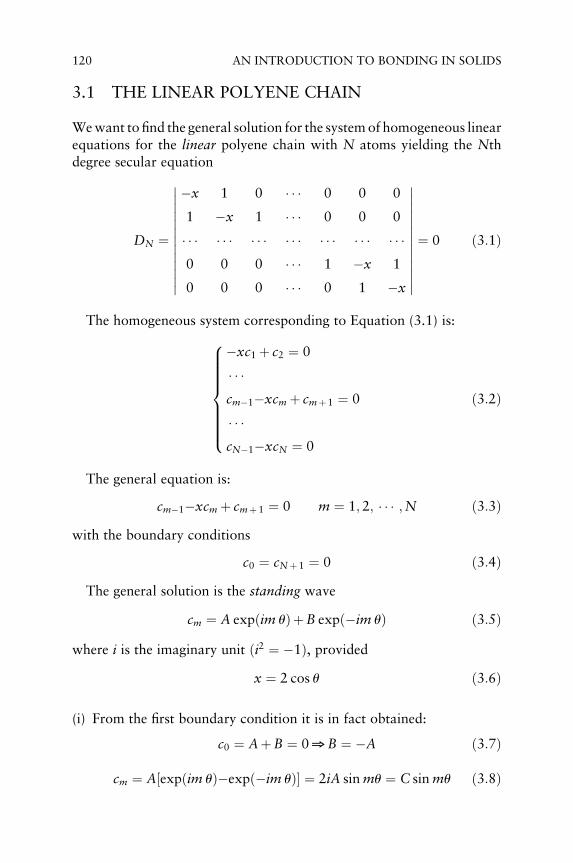
Wewant to find the general solution for the systemof homogeneous linearequations for the linear polyene chain with N atoms yielding the Nthdegree secular equation

DN ¼

�x 1 0 � � � 0 0 0

1 �x 1 � � � 0 0 0

� � � � � � � � � � � � � � � � � � � � �0 0 0 � � � 1 �x 1

0 0 0 � � � 0 1 �x

��

��¼ 0 ð3:1Þ

The homogeneous system corresponding to Equation (3.1) is:

�xc1 þ c2 ¼ 0

� � �cm�1�xcm þ cmþ 1 ¼ 0

� � �cN�1�xcN ¼ 0

8>>>>>>><>>>>>>>:

ð3:2Þ

The general equation is:

cm�1�xcm þ cmþ 1 ¼ 0 m ¼ 1; 2; � � � ;N ð3:3Þwith the boundary conditions

c0 ¼ cNþ 1 ¼ 0 ð3:4ÞThe general solution is the standing wave

cm ¼ A expðim uÞþB expð�im uÞ ð3:5Þ

where i is the imaginary unit ði2 ¼ �1Þ, providedx ¼ 2 cos u ð3:6Þ

(i) From the first boundary condition it is in fact obtained:

c0 ¼ AþB ¼ 0YB ¼ �A ð3:7Þ

cm ¼ A expðim uÞ�expð�im uÞ½ � ¼ 2iA sinmu ¼ C sinmu ð3:8Þ

120 AN INTRODUCTION TO BONDING IN SOLIDS

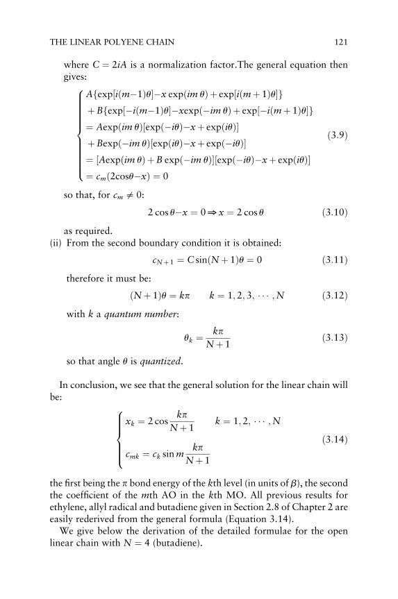
where C ¼ 2iA is a normalization factor.The general equation thengives:

A exp iðm�1Þu½ ��x expðim uÞþ exp iðmþ1Þu½ �f gþB exp �iðm�1Þu½ ��xexpð�im uÞþ exp �iðmþ 1Þu½ �f g¼ Aexpðim uÞ expð�iuÞ�xþ expðiuÞ½ �þBexpð�im uÞ expðiuÞ�xþ expð�iuÞ½ �¼ Aexpðim uÞþB expð�im uÞ½ � expð�iuÞ�xþ expðiuÞ½ �¼ cmð2cosu�xÞ ¼ 0

8>>>>>>>>>><>>>>>>>>>>:

ð3:9Þ

so that, for cm =0:

2 cos u�x ¼ 0Yx ¼ 2 cos u ð3:10Þas required.

(ii) From the second boundary condition it is obtained:

cNþ 1 ¼ C sinðNþ 1Þu ¼ 0 ð3:11Þtherefore it must be:

ðNþ 1Þu ¼ kp k ¼ 1;2; 3; � � � ;N ð3:12Þwith k a quantum number:

uk ¼kp

Nþ 1ð3:13Þ

so that angle u is quantized.

In conclusion, we see that the general solution for the linear chain willbe:

xk ¼ 2 coskp

Nþ 1k ¼ 1; 2; � � � ;N

cmk ¼ ck sinmkp

Nþ 1

8>>>><>>>>:

ð3:14Þ

the first being the p bond energy of the kth level (in units of b), the secondthe coefficient of the mth AO in the kth MO. All previous results forethylene, allyl radical and butadiene given in Section 2.8 of Chapter 2 areeasily rederived from the general formula (Equation 3.14).We give below the derivation of the detailed formulae for the open

linear chain with N ¼ 4 (butadiene).

THE LINEAR POLYENE CHAIN 121

3.1.1 Butadiene N ¼ 4

uk ¼ kp5; xk ¼ 2 cos k

p5; k ¼ 1; 2; 3;4 ð3:15Þ

The roots in ascending order are:

(i) Bonding levels

x1 ¼ 2 cosp5¼ 2 cos36� ¼ 1:618

x2 ¼ 2 cos2p5

¼ 2 cos72� ¼ 0:618

8>>>><>>>>:

ð3:16Þ

(ii) Antibonding levels

x3 ¼ 2 cos3p5

¼ 2 cos108� ¼ �0:618

x4 ¼ 2 cos4p5

¼ 2 cos144� ¼ �1:618

8>>>><>>>>:

ð3:17Þ

which coincide with those of Equations (2.272) of Chapter 2.

For the MOs, we have:

fk ¼Xm

xmcmk ¼ CXm

xmsinmkp5

ð3:18Þ

where C is a normalization factor.Then:

f1 ¼ CX4m¼1

xm sinmp5¼ C x1sin

p5þx2sin

2p5

þx3sin3p5

þx4sin4p5

!

¼ C 0:5878x1þ0:9510x2þ0:9510x3þ0:5878x4ð Þ

¼ 0:3718x1þ0:6015x2þ0:6015x3þ0:3718x4

ð3:19Þ

8>>>>>>><>>>>>>>:


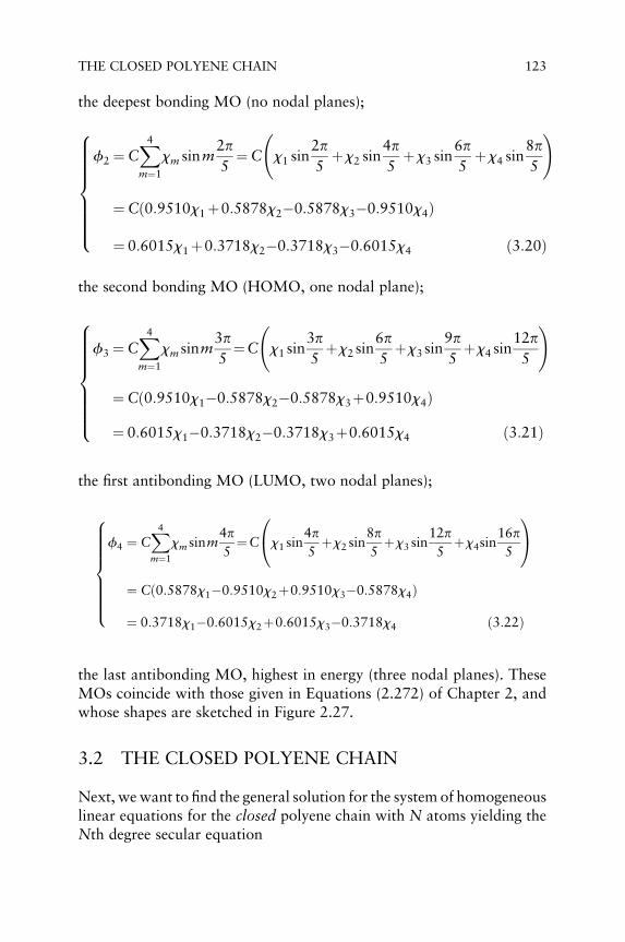
the deepest bonding MO (no nodal planes);

f2 ¼CX4m¼1

xm sinm2p5

¼C x1 sin2p5

þx2 sin4p5

þx3 sin6p5

þx4 sin8p5

!

¼C 0:9510x1þ0:5878x2�0:5878x3�0:9510x4ð Þ

¼ 0:6015x1þ0:3718x2�0:3718x3�0:6015x4 ð3:20Þ

8>>>>>>><>>>>>>>:the second bonding MO (HOMO, one nodal plane);

f3 ¼CX4m¼1

xm sinm3p5¼C x1 sin

3p5þx2 sin

6p5þx3 sin

9p5þx4 sin

12p5

!

¼C 0:9510x1�0:5878x2�0:5878x3þ0:9510x4ð Þ

¼ 0:6015x1�0:3718x2�0:3718x3þ0:6015x4 ð3:21Þ

8>>>>>>><>>>>>>>:the first antibonding MO (LUMO, two nodal planes);

f4 ¼ CX4m¼1

xm sinm4p5¼C x1 sin

4p5þx2 sin

8p5þx3 sin

12p5

þx4sin16p5

0@

1A

¼ C 0:5878x1�0:9510x2þ0:9510x3�0:5878x4ð Þ

¼ 0:3718x1�0:6015x2þ0:6015x3�0:3718x4 ð3:22Þ

8>>>>>>><>>>>>>>:

the last antibonding MO, highest in energy (three nodal planes). TheseMOs coincide with those given in Equations (2.272) of Chapter 2, andwhose shapes are sketched in Figure 2.27.

3.2 THE CLOSED POLYENE CHAIN

Next, wewant to find the general solution for the system of homogeneouslinear equations for the closed polyene chain with N atoms yielding theNth degree secular equation

THE CLOSED POLYENE CHAIN 123

DN ¼

�x 1 0 � � � 0 0 1

1 �x 1 � � � 0 0 0

� � � � � � � � � � � � � � � � � � � � �0 0 0 � � � 1 �x 1

1 0 0 � � � 0 1 �x

��

��¼ 0 ð3:23Þ

The homogeneous system corresponding to Equation (3.23) is:

�xc1 þ c2þ � � � þ cN ¼ 0

� � �cm�1�xcm þ cmþ 1 ¼ 0

� � �c1þ � � � þ cN�1 � xcN ¼ 0

8>>>>>>><>>>>>>>:

ð3:24Þ

The general equation for the coefficients is the same as that for the linearchain:

cm�1�xcm þ cmþ 1 ¼ 0 m ¼ 1;2; � � � ;N ð3:25Þbut with the different boundary conditions:

c0 ¼ cN; c1 ¼ cNþ 1Y cm ¼ cmþN ð3:26Þ

the last being a periodic boundary condition.The general solution is now the progressive wave in complex form:

cm ¼ A expðim uÞ ð3:27Þ

where i is the imaginary unit ði2 ¼ �1Þ, and the general Equation (3.25)gives:

A exp iðm�1Þu½ ��x expðimuÞþ exp iðmþ 1Þu½ �f g ¼ 0

A expðim uÞ expð�iuÞ�xþ expðiuÞ½ � ¼ cmð2 cos u�xÞ ¼ 0

(ð3:28Þ

namely, for cm =0:

x ¼ 2 cos u ð3:29Þ

as before.


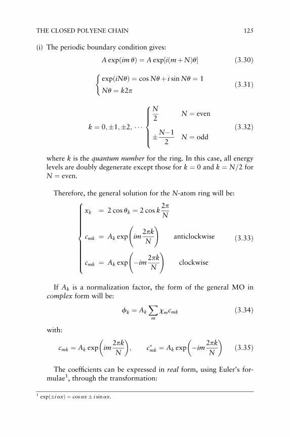
(i) The periodic boundary condition gives:

A expðim uÞ ¼ A exp½iðmþNÞu� ð3:30Þ

expðiNuÞ ¼ cosNuþ i sinNu ¼ 1

Nu ¼ k2p

(ð3:31Þ

k ¼ 0;�1;�2; � � �

N

2N ¼ even

�N�1

2N ¼ odd

8>>>><>>>>:

ð3:32Þ

where k is the quantum number for the ring. In this case, all energylevels are doubly degenerate except those for k ¼ 0 and k ¼ N=2 forN ¼ even.

Therefore, the general solution for the N-atom ring will be:

xk ¼ 2 cos uk ¼ 2 cos k2pN

cmk ¼ Ak exp im2pkN

!anticlockwise

cmk ¼ Ak exp �im2pkN

!clockwise

8>>>>>>>>>>><>>>>>>>>>>>:

ð3:33Þ

If Ak is a normalization factor, the form of the general MO incomplex form will be:

fk ¼ Ak

Xm

xmcmk ð3:34Þ

with:

cmk ¼ Ak exp im2pkN

� �; c�mk ¼ Ak exp �im

2pkN

� �ð3:35Þ

The coefficients can be expressed in real form, using Euler’s for-mulae1, through the transformation:

1 expð�iaxÞ ¼ cosax� i sinax.


cmk�c�mk

2i¼ Ak sinm

2pkN

¼ amk

cmkþ c�mk

2¼ Ak cosm

2pkN

¼ bmk

8>>>><>>>>:

ð3:36Þ

giving the real MOs in the form:

fsk ¼

Xm

xmamk; fck ¼

Xm

xmbmk ð3:37Þ

The previous results for cyclobutadiene and benzene given in Section2.8 of Chapter 2 can be rederived from the general formula(Equation 3.37).We give below the derivation of the detailed formulae for the closed

chain with N ¼ 6 (benzene).

3.2.1 Benzene N ¼ 6

N ¼ 6; uk ¼ k2p6

¼ kp3; xk ¼ 2 cos k

p3; k ¼ 0;�1;�2; 3 ð3:38Þ

The roots in ascending order are:

(i) Bonding levels

x0 ¼ 2

x1 ¼ x�1 ¼ 2 cosp3¼ 1

8><>: ð3:39Þ

(ii) Antibonding levels

x2 ¼ x�2 ¼ 2 cos2p3

¼ �1

x3 ¼ 2 cos3p3

¼ �2

8>>>><>>>>:

ð3:40Þ

which coincide with those of Equations (2.284) of Chapter 2.


For the real coefficients, we have:

amk ¼ A sinmkp3; bmk ¼ A cosm

kp3

ð3:41Þ

with A a normalization factor.For the MOs in real form, we then have:

f0 ¼ fc0 ¼ A

X6m¼1

xm cos u ¼ 1ffiffiffi6

p ðx1þ x2 þx3 þx4 þ x5 þ x6Þ ð3:42Þ

the deepest bonding MO (no nodal planes);

fs1 ¼ A

X6m¼1

xm sinmp3¼ 1

2x1 þ x2�x4�x5ð Þ

fc1 ¼ A

X6m¼1

xm cosmp3¼ 1ffiffiffiffiffiffi

12p x1�x2�2x3�x4 þx5 þ 2x6ð Þ

8>>>>><>>>>>:

ð3:43Þ

the second bonding doubly degenerateMOs (HOMOs, one nodal plane);

fs2 ¼ A

X6m¼1

xm sinm2p3

¼ 1

2x1�x2 þx4�x5ð Þ

fc2 ¼ A

X6m¼1

xm cosm2p3

¼ 1ffiffiffiffiffiffi12

p �x1�x2 þ 2x3�x4�x5 þ 2x6ð Þ

8>>>>><>>>>>:

ð3:44Þ

the first antibonding doubly degenerate MOs (LUMOs, two nodalplanes);

f3 ¼ fc3 ¼ A

X6m¼1

xm cos3p3

¼ 1ffiffiffi6

p ð�x1þx2�x3þx4�x5þx6Þ ð3:45Þ

the last antibondingMO, highest in energy (three nodal planes). TheMOsobtained in this way differ by an orthogonal transformation from those


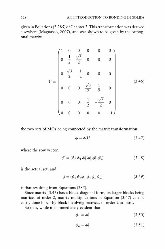
given in Equations (2.285) of Chapter 2. This transformationwas derivedelsewhere (Magnasco, 2007), and was shown to be given by the orthog-onal matrix:

U ¼

1 0 0 0 0 0

01

2

ffiffiffi3

p

20 0 0

0

ffiffiffi3

p

2�1

20 0 0

0 0 0

ffiffiffi3

p

2

1

20

0 0 01

2�

ffiffiffi3

p

20

0 0 0 0 0 �1

0BBBBBBBBBBBBBBBBBBBBBB@

1CCCCCCCCCCCCCCCCCCCCCCA

ð3:46Þ

the two sets of MOs being connected by the matrix transformation:

f ¼ f0U ð3:47Þ

where the row vector:

f0 ¼ ðfc0 f

s1 f

c1 f

s2 f

c2 f

c3Þ ð3:48Þ

is the actual set, and:

f ¼ ðf1 f2f3 f4 f5 f6Þ ð3:49Þ

is that resulting from Equations (285).Since matrix (3.46) has a block-diagonal form, its larger blocks being

matrices of order 2, matrix multiplications in Equation (3.47) can beeasily done block-by-block involving matrices of order 2 at most.So that, while it is immediately evident that:

f1 ¼ fc0 ð3:50Þ

f6 ¼ fc3 ð3:51Þ


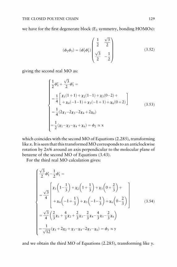
we have for the first degenerate block (E1 symmetry, bonding HOMOs):

ðf2f3Þ ¼ ðfs1f

c1Þ

1

2

ffiffiffi3

p

2ffiffiffi3

p

2�1

2

0BBBBB@

1CCCCCA ð3:52Þ

giving the second real MO as:

1

2fs1 þ

ffiffiffi3

p

2fc1 ¼

¼ 1

4

x1 1þ 1ð Þþx2 1�1ð Þþ x3 0�2ð Þþþ x4 �1�1ð Þþ x5 �1þ1ð Þþx6 0þ2ð Þ

" #

¼ 1

42x1�2x3�2x4 þ 2x6ð Þ

¼ 1

2ðx1�x3�x4 þx6Þ ¼ f2 / x

8>>>>>>>>>>>>>>>>><>>>>>>>>>>>>>>>>>:

ð3:53Þ

which coincides with the secondMO of Equations (2.285), transforminglikex. It is seen that this transformedMOcorresponds to an anticlockwiserotation by 2p/6 around an axis perpendicular to the molecular plane ofbenzene of the second MO of Equations (3.43).For the third real MO calculation gives:

ffiffiffi3

p

2fs1�

1

2fc1 ¼

¼ffiffiffi3

p

4

x1

�1�1

3

�þx2

�1þ 1

3

�þx3

�0þ 2

3

�þ

þ x4

��1þ 1

3

�þ x5

��1� 1

3

�þ x6

�0�2

3

�2666664

3777775

¼ffiffiffi3

p

4

�2

3x1 þ

4

3x2 þ

2

3x3�

2

3x4�

4

3x5�

2

3x6

�


p ðx1 þ2x2 þ x3�x4�2x5�x6Þ ¼ f3 / y

8>>>>>>>>>>>>>>>>>>>>>>><>>>>>>>>>>>>>>>>>>>>>>>:

ð3:54Þ

and we obtain the third MO of Equations (2.285), transforming like y.


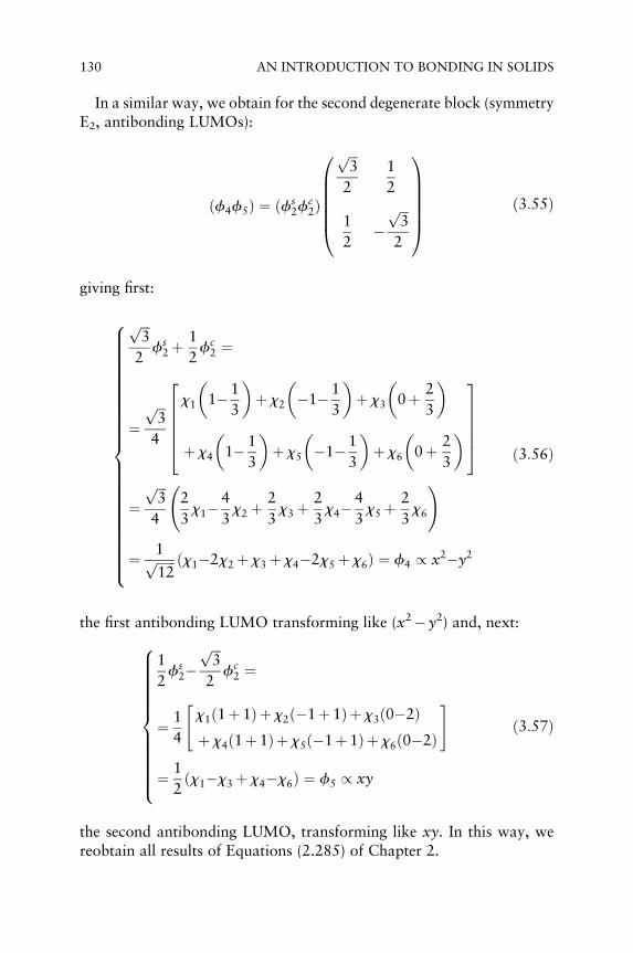
In a similar way, we obtain for the second degenerate block (symmetryE2, antibonding LUMOs):

ðf4f5Þ ¼ ðfs2f

c2Þ

ffiffiffi3

p

2

1

2

1

2�

ffiffiffi3

p

2

0BBBBB@

1CCCCCA ð3:55Þ

giving first:

ffiffiffi3

p

2fs2þ

1

2fc2 ¼

¼ffiffiffi3

p

4

x1

�1� 1

3

�þ x2

��1�1

3

�þ x3

�0þ 2

3

�

þ x4

�1� 1

3

�þ x5

��1� 1

3

�þx6

�0þ 2

3

�266664

377775

¼ffiffiffi3

p

4

2

3x1�

4

3x2 þ

2

3x3 þ

2

3x4�

4

3x5þ

2

3x6

!


p ðx1�2x2þ x3 þx4�2x5 þ x6Þ ¼ f4 / x2�y2

8>>>>>>>>>>>>>>>>>>>>>>><>>>>>>>>>>>>>>>>>>>>>>>:

ð3:56Þ

the first antibonding LUMO transforming like (x2� y2) and, next:

1

2fs2�

ffiffiffi3

p

2fc2 ¼

¼ 1

4

x1 1þ1ð Þþ x2 �1þ 1ð Þþ x3 0�2ð Þþ x4 1þ 1ð Þþx5 �1þ1ð Þþ x6 0�2ð Þ

" #

¼ 1

2x1�x3 þ x4�x6ð Þ ¼ f5 / xy

8>>>>>>>>>>><>>>>>>>>>>>:

ð3:57Þ

the second antibonding LUMO, transforming like xy. In this way, wereobtain all results of Equations (2.285) of Chapter 2.


3.3 A MODEL FOR THE ONE-DIMENSIONALCRYSTAL

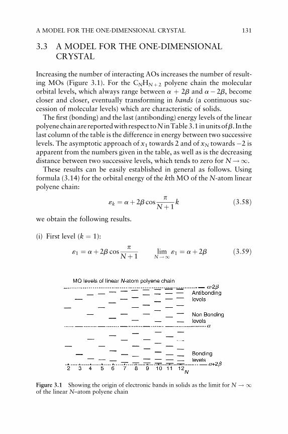
Increasing the number of interacting AOs increases the number of result-ing MOs (Figure 3.1). For the CNHNþ 2 polyene chain the molecularorbital levels, which always range between a þ 2b and a� 2b, becomecloser and closer, eventually transforming in bands (a continuous suc-cession of molecular levels) which are characteristic of solids.The first (bonding) and the last (antibonding) energy levels of the linear

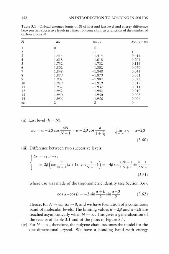
polyenechainarereportedwithrespect toN inTable3.1 inunitsofb. In thelast column of the table is the difference in energy between two successivelevels. The asymptotic approach of x1 towards 2 and of xN towards�2 isapparent from the numbers given in the table, as well as is the decreasingdistance between two successive levels, which tends to zero for N!1.These results can be easily established in general as follows. Using

formula (3.14) for the orbital energy of the kth MO of theN-atom linearpolyene chain:

«k ¼ aþ 2b cosp

Nþ 1k ð3:58Þ

we obtain the following results.

(i) First level (k ¼ 1):

«1 ¼ aþ 2b cosp

Nþ 1lim

N!1«1 ¼ aþ 2b ð3:59Þ

Figure 3.1 Showing the origin of electronic bands in solids as the limit for N ! 1of the linear N–atom polyene chain

A MODEL FOR THE ONE-DIMENSIONAL CRYSTAL 131

(ii) Last level (k ¼ N):

«N ¼ aþ 2b cospN

Nþ 1¼ aþ 2b cos

p1þ 1

N

limN!1

«N ¼ a�2b

ð3:60Þ(iii) Difference between two successive levels:

D« ¼ «kþ1�«k

¼ 2b

�cos

pNþ 1

ðkþ1Þ�cosp

Nþ 1k

�¼ �4b sin

p2

2kþ1

Nþ 1sin

p2

1

Nþ1

8><>:

ð3:61Þwhere use was made of the trigonometric identity (see Section 3.6):

cos a�cos b ¼ �2 sinaþb

2sin

a�b

2ð3:62Þ

Hence, forN!1; D«!0, and we have formation of a continuousband of molecular levels. The limiting values aþ 2b and a�2b arereached asymptotically whenN!1. This gives a generalization ofthe results of Table 3.1 and of the plots of Figure 3.1.

(iv) For N!1, therefore, the polyene chain becomes the model for theone-dimensional crystal. We have a bonding band with energy

Table 3.1 Orbital energies (units of b) of first and last level and energy differencebetween two successive levels in a linear polyene chain as a function of the number ofcarbon atoms N

N xN xNþ 1 xNþ 1� xN

1 0 02 1 �1 13 1.414 �1.414 0.4144 1.618 �1.618 0.2045 1.732 �1.732 0.1146 1.802 �1.802 0.0707 1.848 �1.848 0.0468 1.879 �1.879 0.0319 1.902 �1.902 0.02310 1.919 �1.919 0.01711 1.932 �1.932 0.01112 1.942 �1.942 0.01013 1.950 �1.950 0.00814 1.956 �1.956 0.0061 2 �2 0


ranging from aþ 2b to a, and an antibonding band with energyranging from a to a�2b, which are separated by the so-called Fermilevel, the top of the bonding band occupied by electrons. It isimportant to notice that using just one b, equal for single and doublebonds as we have done, there is no band gap between bonding andantibonding levels (Figure 3.2). If we admit jbdj > jbsj, as reasonableand done by Lennard-Jones in his original work (1937), we have aband gap D ¼ 2ðbd�bsÞ, which is of great importance in the prop-erties of solids. Figure 3.3 shows the origin of this band gap. In thefigure, «F is the Fermi level, that is the negative of minimum energyrequired to ionize the system.Metals and covalent solids, conductorsand insulators, semiconductors, can all be traced back to themodel ofthe infinite polyene chain extended to three dimensions (McWeeny,1979).

3.4 ELECTRONIC BANDS IN CRYSTALS

FromEquation (3.61),we candefine adensity of energy levels ordensity ofstates N(«) in the crystal as D«�1.N(«) is a function giving the number or

Figure 3.2 Electronic bands in linear polyene chain (single b)

ELECTRONIC BANDS IN CRYSTALS 133

levels (or states) in an infinitesimal range of «, and is quantitatively definedas:

Nð«Þ ¼ @k

@«¼ @«

@k

� ��1

¼ � 1

2b

Nþ1

pcosec

pkNþ 1

ð3:63Þ

In fact, from Equation (3.14):

« ¼ aþ 2b cospk

Nþ 1ð3:64Þ

@«

@k¼ �2b

pNþ 1

sinpk

Nþ 1ð3:65Þ

@«

@k

� ��1

¼ � 1

2b

Nþ 1

pcosec

pkNþ 1

ð3:66Þ

or, by expressing k as f(«):

cospk

Nþ 1¼ «�a

2bð3:67Þ

Figure 3.3 Electronic bands in linear polyene chain (double b)


pkNþ 1

¼ cos�1 «�a

2b

� �ð3:68Þ

where �1 denotes the inverse function.Hence, remembering from elementary analysis that:

d cos�1u

d u¼ �ð1�u2Þ�1=2 ð3:69Þ

we have:

k ¼ Nþ 1

pcos�1 «�a

2b

� �ð3:70Þ

@k

@«¼ � 1

2b

Nþ 1

p1� «�a

2b

!224

35�1=2

¼ � 1

2b

Nþ 1

psin2

pkNþ 1

!�1=2

¼ � 1

2b

Nþ 1

pcosec

pkNþ 1

8>>>>>>><>>>>>>>:

ð3:71Þ

the same result as before.To introduce further details of the theoryof solids in an elementaryway,

we can resort to the results given in Section 3.2 for the closed chainwithNatoms.Wehave shown there that the general solution in complex form forthe N-atom closed chain with N ¼ odd is:

xk ¼ 2 cos2pkNþ1

k ¼ 0;�1;�2; � � � ;� N�1

2

!

cmk / exp 2pimk

N

!8>>>>><>>>>>:

ð3:72Þ

where i is the imaginary unit. Apart from the ground state ðk ¼ 0Þ,roots (3.72) occur in pairs, each level being hence doubly degenerate.Let consider as an example the cases N ¼ 5 and N ¼ 15. We have the

numerical results of Table 3.2 which are plotted in Figure 3.4.For solids, the quantum number k is replaced by the wave vector k:

ka ¼ 2pkN

; k ¼ 0;� pa

2

N; � � � ;� p

a1� 1

N

� �ð3:73Þ

where a is the lattice spacing.


For N!1, we have the plots sketched in Figure 3.5, that on the leftgiving x(k) versus k, that on the right the energy levels «ðkÞ versus thedensity of states N(«), and where the Fermi level «F is apparent.In the crystal, the periodic potential of the nuclei will perturb the energy

levels, removing the double degeneracy of the two states corresponding to�p=a, the splittingmanifesting itself as a band gap in the energy spectrum.For the values of k for which l ¼ 2a this originates discontinuities in thespectrum, giving gaps that divide the jkj space into zones called Brillouinzones. The region from jkj ¼ 0 is the first break, called the first Brillouinzone, from there up to the second break is the second Brillouin zone, andso on. These zones have the dimensions of reciprocal length, and areschematically plotted in Figure 3.6.

Table 3.2 Roots of the closed chains for N ¼ 5 and N ¼ 15

N ¼ 5 N ¼ 15

k xk ¼ 2 cos 2pk5 k xk ¼ 2 cos 2pk15

0 2 0 2�1 0.618 �1 1.827�2 �1.618 �2 1.338

�3 0.618�4 �0.219�5 �1�6 �1.618�7 �1.956

Figure 3.4 Plots of the roots for the closed chain withN ¼ 5 (left) and N ¼ 15(right)


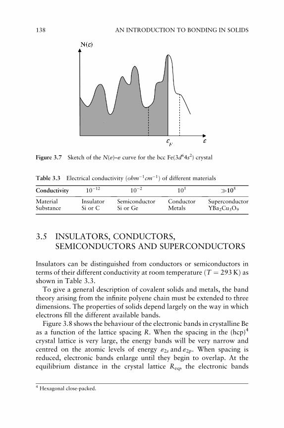
Figure 3.7 gives a sketch of theN(«)–« curve for the d-band of the bcc2

Fe(3d64s2) crystal as calculated numerically via the APW3 method byWood (1962).

Figure 3.5 Energy levels versusk (left), andenergy levels versusdensityof states (right)

2 Body-centred cubic.3 The APW (augmented planewave) methodwas devised by Slater (1937, 1965), and is based on

the solution of the Schr€odinger equation for a spherical periodic potential using an expansion ofthe wavefunction in terms of solutions of the atomic problem near the nucleus, and an expansionin plane waves outside a predetermined sphere in the crystal.

Figure 3.6 One-dimensional Brillouin zones


3.5 INSULATORS, CONDUCTORS,SEMICONDUCTORS AND SUPERCONDUCTORS

Insulators can be distinguished from conductors or semiconductors interms of their different conductivity at room temperature ðT ¼ 293 KÞ asshown in Table 3.3.To give a general description of covalent solids and metals, the band

theory arising from the infinite polyene chain must be extended to threedimensions. The properties of solids depend largely on the way in whichelectrons fill the different available bands.Figure 3.8 shows the behaviour of the electronic bands in crystalline Be

as a function of the lattice spacing R. When the spacing in the (hcp)4

crystal lattice is very large, the energy bands will be very narrow andcentred on the atomic levels of energy «2s and «2p. When spacing isreduced, electronic bands enlarge until they begin to overlap. At theequilibrium distance in the crystal lattice Req, the electronic bands

Figure 3.7 Sketch of the N(«)–« curve for the bcc Fe(3d64s2) crystal

Table 3.3 Electrical conductivity ðohm�1cm�1Þ of different materials

Conductivity 10�12 10�2 105 �105

Material Insulator Semiconductor Conductor SuperconductorSubstance Si or C Si or Ge Metals YBa2Cu3O9

4 Hexagonal close-packed.


originating from the 2s and 2p atomic levels will overlap, while the inner1sbandwill still be very separated because of its large difference in energy.Each Be ð1s22s2Þ atom will contribute four electrons to the solid. Twoelectrons come from the inner shell and are sufficient to fill the 1s bandcompletely. The other two electrons come from the valence 2s orbital, andsuffice to fill the 2s band completely. At large lattice spacings, the groundstate of the solid will have a completely filled 1s band and a completelyfilled 2s band, and therewill be a gap between the 2s filled band and the 2pempty band. At variance with what occurs in metals, a large amount ofenergy, theD2s�2p band gap,will be needed to transfer electrons fromfilledto empty orbitals, so that solid Be with a large value of R will be aninsulator. However, at Req in solid Be, the two 2s and 2p bands partiallyoverlap and the crystal orbitalswill have both s andp character, so that theoverlapping bands can now contain eight electrons from each atom. Thetwo electrons that each Be atom can contribute at the valence level willonly partially fill the combined bands, so that there will be no energy gapamong occupied and empty levels, and solid Be at its equilibrium latticedistance Req will be a typical metal.The fact that a solid is a metal or a nonmetal will therefore depend on

three factors: (i) the separation of the orbital energies in the free atom;(ii) the lattice spacing; and (iii) the number of electrons provided by eachatom. For a realistic description of the three-dimensional crystal, wemusttherefore extend our simpleH€uckel theory5 in two respects. First, wemustconsidermore than a single type of AOs (e.g. 2s, 2p, 3d, � � � ), and, second,we must consider more than an electron per atom. By increasing the

Figure 3.8 Overlap of electronic bands in solid Be

5 In solid state theory called the tight-binding approximation (TBA) (see Table 3.4).

INSULATORS, CONDUCTORS, SEMICONDUCTORS 139

external pressure on a solid, namely by compressing it, will reduce thelattice spacing, widening the bands, so that under sufficient pressure, allsolids will display metallic character (as first claimed by J.D. Bernal,quoted in Wigner and Huntington, 1935; see also Yakovlev, 1976).A covalent solid (insulator, such as diamond, pure state carbon) has

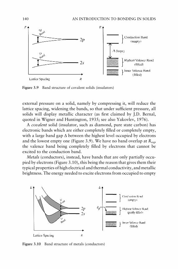
electronic bands which are either completely filled or completely empty,with a large band gap D between the highest level occupied by electronsand the lowest empty one (Figure 3.9). We have no band overlap at Req,the valence band being completely filled by electrons that cannot beexcited to the conduction band.Metals (conductors), instead, have bands that are only partially occu-

pied by electrons (Figure 3.10), this being the reason that gives them theirtypical properties of high electrical and thermal conductivity, andmetallicbrightness. The energy needed to excite electrons from occupied to empty

Figure 3.9 Band structure of covalent solids (insulators)

Figure 3.10 Band structure of metals (conductors)


bands is extremely small, their energy being readily distributed over theentiremetal because of fullyMOdelocalization. Furthermore, ametal canabsorb light of any wavelength. The highest valence band is only partiallyfilled, and electrons may flow easily under the action of an external field,except for the collisions with the positive ions of the lattice. Increasingtemperature increases lattice vibrations and electron collisions, so thatelectrical conductivity decreases.Semiconductors have a small band gap, 60–100kJmol�1, namely

0.6–1 eV for Ge or Si (Figure 3.11). The electrons of the last valenceband are easily excited to the conduction band (empty) under the effect oftemperature ðkT � «C�«FÞ or light ðhn � «C�«FÞ, the latter effect beingknownas photoconductivity. The electronic population in the conductionband will increase with temperature according to the statistical equilib-rium described by the Fermi–Dirac statistics, so that conductivity willincrease with temperature (the opposite of what was found for metals).Besides conduction due to the electrons thermally excited to the

conduction band (n-type, negative charge), there may be conduction dueto vacancies occurring in the valence band (p-type, where p stands for apositive hole). Germanium and silicon are typical intrinsic semiconduc-tors (left-hand side of Figure 3.11), whose properties are due to the pureelements. But also of great importance are the so-called impurity semi-conductors, where small amounts of impurity in a perfect crystal latticecan modify the structure of the Brillouin zones, giving products whoseproperties may be of commercial interest. The ’doping’ of silicon orgermanium can be done using elements with one more electron in theirvalence shell, such as phosphorus or arsenic, or elements with one less

Figure 3.11 Band structure of intrinsic and doped semiconductors

INSULATORS, CONDUCTORS, SEMICONDUCTORS 141

electron in their valence shell, such as gallium or indium6. Conductionnow arises from excitation of the electrons out of (n-type) or into (p-type)the impurity levels (right-hand side of Figure 3.11). Formore informationthe reader is referred to elsewhere (see, for instance,Murrell et al., 1985).As we have seen, at low temperatures, resistance to the current flow

decreases for all crystal conductors (metals) and, therefore, electricconductivity increases. At a given critical temperature Tc, resistancedisappears completely and the metal becomes a superconductor, with aninfinitely large conductivity (Figure 3.12). Formetals, this occurs at ratherlow temperatures (<30K), but Bednorz andM€uller (1986)7 prepared newsubstances exhibiting high-temperature superconductivity (above 77K,the boiling temperature of liquid N2). These are alloys containing Cu, O,La (where La may be replaced by Ba, Sr and Y) with a perovskite(La2CuO4) lattice structure.They are structurally homogeneous, perfectly diamagnetic, with a very

small band gap, D less than 0.1 eV. These materials were prepared bydoping perovskites in two ways, either by introducing oxygen-deficientcompounds (such as La2CuO4�x) or by replacing La by other atoms X(such as Ba, Sr, Y). On the theoretical side, Mattheiss (1987) did ab initiocalculations of the electronic band structure of tetragonal La2CuO4 andofsuperconductors derivatives of it, such as La2�yXyCuO4, that throw somelight on the factors determining superconductivity at high temperature.The electronic bands at the Fermi surface show a substantially p-char-acter. These p AOs give strong s bonds with the 3d orbitals of Cu of

Figure 3.12 Plot of resistance versus temperature for common metals

6 Ground state valence electron configurations of the elements are: Si(3s23p2) and Ge(4s24p2), P(3s23p3) and As(4s24p3), Ga(4s24p) and In(5s25p).7 1987 Nobel Prize for Physics.


appropriate symmetry8. The breathing lattice vibrations of the fourcoplanar O atoms are strongly coupled with the electron conductionband at «F, giving a high value for the coupling electron–phonon constantl that occurs in the Bardeen–Cooper–Schrieffer (BCS) theory of super-conductivity (Tinkham, 1975), with a band gap at «F ð0:2�0:5 eVÞdetermining a large value of the deformation potential ð1:6�3:9 eV=A

� Þ.Because of the small mass of the oxygen atoms and the high-frequencyv oflattice vibrations, the pre-exponential factor in the BCS equation for Tc ismagnified, thus generating the high Tc values observed for these com-pounds. The effect is magnified for X ¼ Sr;Ba.To end this section, it may be useful to the reader to give a table

collecting some analogies between molecular and solid state theory(Table 3.4). The table is taken from Albright et al. (1985), and is usefulin connecting quantum theorist terminology to that of solid statephysicists.

3.6 APPENDIX: THE TRIGONOMETRIC IDENTITY

The trigonometric identity (Equation 3.62) can be easily derived asfollows. We start from the well-known trigonometric formulae:

cosðx�yÞ ¼ cos x cos yþ sin x sin y ð3:74Þ

cosðxþ yÞ ¼ cos x cos y�sin x sin y ð3:75Þ

Table 3.4 Connection between molecular and solid state terminologies

Molecular theory Solid state theory

MO (molecular orbital) Bloch orbital (crystal orbital)Energy levels Energy bandHOMO Valence bandLUMO Conduction bandHOMO/LUMO energy difference Band gapH€uckel theory Tight-binding approximation (TBA)MO models with electron repulsion H€uckel–Hubbard HamiltonianResonance integral b Hopping integral tJahn–Teller distortion Peierls distortionHigh spin Magnetic materialLow spin Nonmagnetic material

8 TheOhoctahedral symmetryofCu is distorted to aD4h tetragonal symmetry,with four stronger

planar dp–s bonds and two weaker apical dp–s bonds.

APPENDIX: THE TRIGONOMETRIC IDENTITY 143

sinx siny ¼ 1

2cosðx�yÞ�cosðxþ yÞ½ � ð3:76Þ

Subtracting Equation (3.75) from (3.74), immediately gives (3.76). Ifwe put:

x�y ¼ a

xþ y ¼ b

(ð3:77Þ

then:

x ¼ aþb

2

y ¼ �a�b

2

8>>>><>>>>:

ð3:78Þ

and, substituting in Equation (3.76):

sinaþb

2sin �a�b

2

� �¼ 1

2ðcos a�cos bÞ ð3:79Þ

so that we obtain Equation (3.62):

cos a�cos b ¼ �2 sinaþb

2sin

a�b

2ð3:80Þ

since sin x is an odd function of x, namely:

sinð�xÞ ¼ �sinx ð3:81Þ


models for bonding in chemistry (magnasco/models for bonding in chemistry) || an introduction to...

Documents