models, race, and the law
TRANSCRIPT

744
THE YALE LAW JOURNAL FORUM M A R C H 8 , 2 0 2 1
Models, Race, and the Law Moon Duchin & Douglas M. Spencer
abstract. Capitalizing on recent advances in algorithmic sampling, “The Race-Blind Future of Voting Rights” explores the implications of the long-standing conservative dream of certified race neutrality in redistricting. Computers seem promising because they are excellent at not taking race into account—but computers only do what you tell them to do, and the rest of the authors’ apparatus for measuring minority electoral opportunity failed every check of robustness and nu-merical stability that we applied. How many opportunity districts are there in the current Texas state House plan? Their methods can give any answer from thirty-four to fifty-one, depending on invisible settings. But if we focus only on major technical flaws, we might miss the fundamental fact that race-blind districting would devastate minority political opportunity no matter how it is deployed, just due to the mathematics of single-member districts. In the end, the Article develops an extreme interpretation of a dubious idea proposed by Judge Easterbrook through an empirical study that is unsupported by the methods.
introduction
The Voting Rights Act of 1965 (VRA) guarantees that all American citizens, regardless of race or ethnicity, should have an equal opportunity to participate in the political process and to elect representatives of their choice.1 The VRA fre-quently interacts with single-member districts, which serve as the electoral sys-tem for congressional and nearly all state legislative races and are the go-to rem-edy in local VRA enforcement. It has long been known in the redistricting literature that random boundary placement puts minorities at a major structural disadvantage.2 Single-member districts can secure electoral opportunity for mi-norities, but only if the minority population is sufficiently concentrated and the
1. 52 U.S.C. § 10301(b) (2018).
2. See, e.g., Bernard Grofman, For Single-Member Districts, Random is Not Equal, in REPRESENTA-
TION AND REDISTRICTING ISSUES 55, 55-58 (Bernard Grofman, Arend Lijphart, Robert McKay

models, race, and the law
745
boundaries are favorably aligned. The ability of the VRA to remediate historical discrimination and underrepresentation thus depends on proactive redistricting. As a matter of practice, when a set of districts empowers minority communities to elect representatives in rough proportion to their population, courts have held the promise of political equality to have been fulfilled.3 However, proportionality has functionally operated as a ceiling even when viewed as normatively desira-ble: White voters will never be represented by less than their share of the popu-lation while minority communities nearly invariably will.4
In The Race-Blind Future of Voting Rights (henceforth, the Article), Jowei Chen and Nicholas Stephanopoulos sketch out a less proactive future of district-ing, including a mechanism that stands to needlessly sabotage minority political power and undermine the signal remedial goal of the VRA.5 The authors devote their Article to delineating a new baseline of opportunity provided by a random-ized redistricting protocol that operates with no regard to race.6 Their project is strategic and pragmatic, motivated by the prediction that an increasingly con-servative Supreme Court is likely to effect “avulsive change” for the VRA in the near term, quite possibly by dropping any role for rough proportionality and elevating race-blind mapping as a new ideal.7 Their Article thus seeks to provide a roadmap for voting-rights advocates to navigate a new nominally race-blind landscape.
To present their approach as a manageable standard, Chen and Stephanop-oulos go big—modeling voter preferences in 1,903 districts and evaluating 38,000 districting plans spanning 19 states—and describe their outputs as the race-blind baseline, full stop. Their particular setup is said to be capable of cap-turing the full dynamics of non-racial redistricting.
& Howard Scarrow eds., 1982). Jowei Chen also coauthored a ground-breaking study of the interplay of geography and this well-known majority seat bonus. See Jowei Chen & Jonathan Rodden, Unintentional Gerrymandering: Political Geography and Electoral Bias in Legislatures, 8 Q.J. POL. SCI. 239 (2013).
3. See, e.g., Johnson v. De Grandy, 512 U.S. 997, 1000 (1994); see also Ellen D. Katz, Margaret Aisenbrey, Anna Baldwin, Emma Cheuse & Anna Weisbrodt, Documenting Discrimination in Voting: Judicial Findings Under Section 2 of the Voting Rights Act Since 1982, 39 U. MICH. J.L. REFORM 643, 654-60 (2006) (documenting and analyzing section 2 decisions).
4. See, e.g., Nicholas O. Stephanopoulos, The Relegation of Polarization, 83 U. CHI. L. REV. ONLINE 160, 168 (2017) (explaining that a “more accurate statement of the [dominant theory of vote dilution] is that minority voters should be able to elect their preferred candidates to the extent permitted by their geographic distribution up to a ceiling of proportionality”).
5. Jowei Chen & Nicholas O. Stephanopoulos, The Race-Blind Future of Voting Rights, 130 YALE
L.J. 862 (2021). 6. Id. 7. Id. at 947.

the yale law journal forum March 8, 2021
746
We find that most—though not all—enacted state-house plans overrepresent minority voters relative to the race-blind baseline. For ex-ample, numerous plans in the Deep South include substantially more Af-rican American opportunity districts than would typically emerge from a nonracial redistricting process, while a few plans in the Border South in-clude fewer such districts. Similarly, several western states feature extra Hispanic opportunity districts compared to the race-blind baseline, while only one western state underrepresents Hispanic voters.8
As we show below, the authors’ methodology does not warrant these kinds of conclusive statements, much less the slippage into the unmistakably norma-tive language of over- and underrepresentation.
We certainly share the authors’ enthusiasm about the burgeoning ensemble method. The central counterfactual problem in vote dilution law for many dec-ades has been that of conceptualizing the undiluted baseline, or understanding how districts might convert votes into seats in a state of nature, absent manipu-lation. In recent years, algorithms that generate large samples of “ensembles” of plausible districting plans have been increasingly used to approach that question. Using ensembles made to conform to legal rules, but without regard to race or partisan data, can provide a non-gerrymandered baseline. Unfortunately, the ap-proach taken by Chen and Stephanopoulos does not conform to best practices in mathematical modeling.9
First, the authors’ ambitious scope leads them to take many shortcuts in methodology as they build their ensembles and label of opportunity. They bor-row tools from mathematical and statistical modeling (notably the randomized districting algorithm developed in the research group that one of us runs10) but do not provide a detailed description of their design choices; do not report any convergence metrics to confirm that their ensembles of districting plans are rep-resentative of any particular weighting of plans; and do not provide any control of errors that propagate through their workflow, especially through their idio-syncratic use of ecological inference.
8. Id. at 867. 9. One attempt to model the Voting Rights Act (VRA) compliance in a Markov chain can be
found in a collaborative effort by data scientists and a voting-rights attorney, see Amariah Becker, Moon Duchin, Dara Gold & Sam Hirsch, Computational Redistricting and the Voting Rights Act, METRIC GEOMETRY & GERRYMANDERING GROUP (2020), https://mggg.org/VRA [https://perma.cc/8WJ4-KRPD].
10. This Markov chain algorithm, called recombination or ReCom, is discussed at more length infra Part III. 2 and Appendix A.1. For a detailed discussion of ReCom, see Daryl DeFord, Moon Duchin & Justin Solomon, Recombination: A Family of Markov Chains for Redistricting, METRIC GEOMETRY & GERRYMANDERING GROUP (Mar. 27, 2020), https://mggg.org/ReCom .pdf [https://perma.cc/6N3Z-B5G7].

models, race, and the law
747
There are quite a few junctures where their modeling decisions should be flagged. For example, the nineteen states under consideration all have different statutory and constitutional rules for redistricting. Therefore, a one-size-fits-all modeling approach cannot come close to the mark of capturing legal nuance. This is not simply a question of whether to take each rule or principle into ac-count, but how to operationalize that priority. For example, the legal language around county preservation is markedly different across these states: Texas men-tions county preservation,11 North Carolina12 and Ohio13 have extremely specific language about how to measure it, and Delaware14 and Illinois15 do not have any county preservation rules at all. Nevertheless the same kind of (very strong) county filter is applied by Chen and Stephanopoulos in generating districts in all states—the details, impacts, and alternatives are left completely undiscussed even though the particular filter they use sacrifices the properties needed for rep-resentative sampling. Perhaps more fundamentally, the authors rely on a single presidential election to infer voter preferences—Obama versus Romney 2012—immediately decoupling their findings from VRA practice where attorneys would never claim to identify minority opportunity based on Obama’s reelection numbers alone. Beyond this, the authors consider only a single plausible defini-tion of opportunity district; they do not compare their “opportunity” label against the ground truth of recent district performance; and they provide no sig-nificant robustness checks at any step in their modeling. Because the authors
11. TX. CONST. art. 3, § 26 (requiring that state house districts be apportioned among the coun-ties, and that counties not be split to the extent possible).
12. Stephenson v. Bartlett, 582 S.E.2d 247, 250 (N.C. 2003) (interpreting Article 2 of the state constitution that “no county shall be divided” to permit county splits for VRA compliance or when necessary to comply with the one-person-one-vote standard so long as county group-ings are minimized and resulting districts fall within five percent of population equality).
13. OHIO CONST. art. 19, § 2(B)(5) (“Of the eighty-eight counties in this state, sixty-five counties shall be contained entirely within a district, eighteen counties may be split not more than once, and five counties may be split not more than twice.”); id. § 2(B)(7) (“No two congres-sional districts shall share portions of the territory of more than one county, except for a county whose population exceeds four hundred thousand.”); id. § 2(B)(8) (“The authority drawing the districts shall attempt to include at least one whole county in each congressional district. This division does not apply to a congressional district that is contained entirely within one county or that cannot be drawn in that manner while complying with federal law.”).
14. DEL. CODE tit. 29, § 804 (“In determining the boundaries of the several representative and senatorial districts within the State, the General Assembly shall use the following criteria. Each district shall, insofar as is possible: (1) Be formed of contiguous territory; (2) Be nearly equal in population; (3) Be bounded by major roads, streams or other natural boundaries; and (4) Not be created so as to unduly favor any person or political party.”).
15. ILL. CONST. art. 4, § 3(a) (“Legislative Districts shall be compact, contiguous and substantially equal in population. Representative Districts shall be compact, contiguous, and substantially equal in population.”).

the yale law journal forum March 8, 2021
748
package their series of complex and computationally intensive functions into a single statistic (the median number of opportunity districts) with very little dis-cussion about their modeling choices, readers may not appreciate the extent to which many of the ingredients are arbitrary, approximate, or numerically unsta-ble. We unpack some of the workflow complexity in Table 2. Do these many choices have effects that cancel out in the end somehow, leaving the finding of over- or underrepresentation intact even if the numbers shift? Do their design choices systematically bias estimates upwards or downwards relative to what would be possible if more elections were taken into account or state laws were handled differently? Chen and Stephanopoulos, when they do address these questions, do so glibly.16
Second, the authors misuse the ensembles that they do generate. Ensembles are not suited to identifying a single ideal value of a score, as Chen and Stepha-nopoulos implicitly do by assigning a designation of under- or overrepresenta-tion based on the median value alone.17 Rather, ensembles are a powerful tool for understanding baseline ranges for valid districting plans and are useful for clari-fying decisionmaking tradeoffs. As the Supreme Court held in 1994, “no single statistic provides courts with a shortcut to determine whether a set of single-member districts unlawfully dilutes minority strength.”18 The single statistic presented by Chen and Stephanopoulos is no exception.
One of the challenges of introducing novel technical methods in a law review is that the blueprints that are especially important for validation—the details of algorithm design, the magnitude of uncertainty, convergence metrics, alternative specifications, and other robustness checks—are not likely to draw needed scru-tiny from law review editors or indeed to hold the attention of most readers. The temptation is thus to gloss over or omit these technical details altogether, even in an eighty-six-page article and its fifty-three-page appendix. But transparency
16. It is of course insufficient to assert that design choices are applied for measuring opportunity in both the enacted plan and its comparator maps, as the authors do. Chen & Stephanopoulos, supra note 5, at 901 n.174 (“Any idiosyncrasies in our particular ecological inference run are reflected in the numbers of opportunity districts we report for both the enacted plans and the simulated [sic] maps.”). We demonstrate this inadequacy in infra Figure 5, where we show that instability may affect the measurement of the enacted plan while leaving the ensemble unchanged.
17. For a discussion of their reliance on the median, see infra Section II.2. It was sleight of hand of just this kind—treating a single number based on piles of political modeling choices as an authoritative indicator—that earned the memorable label of sociological gobbledygook. Tran-script of Oral Argument at 40, Gill v. Whitford, 138 S. Ct. 1916 (No. 16-1161) (“CHIEF JUS-TICE ROBERTS: . . . the whole point is you’re taking these issues away from democracy and you’re throwing them into the courts pursuant to, and it may be simply my educational back-ground, but I can only describe as sociological gobbledygook.”).
18. Johnson v. De Grandy, 512 U.S. 997, 1020-21 (1994).

models, race, and the law
749
is all the more important for a project that has not been subject to rigorous peer review. This worry about law review publication is not new. Nearly twenty years ago, Lee Epstein and Gary King wrote an important piece in which they reviewed the legal literature and sounded the alarm that “the current state of empirical legal scholarship is deeply flawed.”19 The lack of attention to sound methodology, they warned, would lead readers to “learn considerably less accurate information about the empirical world than the studies’ stridently stated, but overly confi-dent, conclusions suggest.”20
This is exactly what generates our grave concerns about the current Article and its placement in a flagship law review. Chen and Stephanopoulos’s style of leveraging technical tools while ignoring the scientific standards surrounding their development and deployment risks creating an unnecessarily muddy legal terrain. And the stakes are high: they have provided a recipe that may well dev-astate electoral opportunity for minority groups just as public opinion and vot-ing behavior are pushing the other way.
In sum, we find that The Race-Blind Future of Voting Rights is a provocative proof of concept that stands on a shaky empirical foundation. The Article uses the promising ensemble method of random district generation to deliver a baseline for minority electoral opportunity; this Response both flags technical issues and questions the conceptual alignment of the methods with their application to vot-ing rights law.
Overview
In Part I we will discuss the nonlinear effects of winner-take-all districting, explaining that the mathematics of districts induces a major representational dis-advantage for any group in the numerical minority. Minority groups are there-fore systematically disfavored by single-member districts just as they are by at-large plurality voting. The law must take up the challenge of counteracting these effects for groups that are protected from disparate treatment. We argue that the difficult task of remedial district design becomes excruciating if we gauge success by standards that ignore, or at least proclaim to ignore, the very feature that trig-gers the obligation to protect.
In Part II we trace the intuition that algorithmic methods can generate a baseline for voting-right opportunity through law and policy literature, culmi-nating in the proposal by Judge Frank Easterbrook of the Seventh Circuit that is cited as motivation by Chen and Stephanopoulos. We outline the promise of
19. Lee Epstein & Gary King, The Rules of Inference, 69 U. CHI. L. REV. 1, 6 (2002). 20. Id. at 6-7.

the yale law journal forum March 8, 2021
750
ensembles to address foundational questions about vote dilution, and we illus-trate why the median should not be elevated to an ideal, as is strongly implied by the authors’ labels of under- and overrepresentation.
In Part III we describe the logic of building ensembles using Markov chain Monte Carlo, or MCMC. The main benefit of using MCMC to find a baseline is that it is built to draw representative samples of all valid districting plans according to a desired weighting, or “target distribution.” A mere sample, with no infor-mation about its distribution, offers no evidence at all—total agreement among your Facebook friends does not say much about national public opinion. A close read of the Article coupled with a close inspection of the authors’ replication ma-terials reveals their conflation of various methodologies and their inattention to bottlenecks that block their ability to sample in a representative manner.
In Part IV we provide several concrete data demonstrations that test the soundness of the Article’s findings, using Texas as an illustrative example. We find that a significant driver of instability is the manner of employing ecological inference (EI) to estimate candidate preference by race. Though EI is a valid family of estimation methods, it should be used with caution because of well-documented limitations in precision and untestable questions of model selec-tion.21 The authors do not defend their EI modeling choices or include any un-certainty estimates, generating instability that propagates through their work-flow and implicates their analysis. For example, we count fifty-one seats (of 150) in the Texas state House that have demonstrably provided electoral opportunity for minority candidates of choice following the 2010 Census. Chen and Stepha-nopoulos report that forty-six seats currently meet their definition of minority opportunity district (MOD). But merely toggling four settings between the au-thors’ EI setup and alternative setups we commonly find in expert reports—while maintaining their precise definition of MOD and using the same R pack-age they used to run EI—we were able to make the measured number of oppor-tunity districts in the enacted plan itself vary from thirty-four to fifty-one seats, as shown in Figure 5. This does not mean that EI should be discarded, but its role in the Article’s definition of MOD is far too central and too hard-edged. A definition that uses richer electoral history would be far more robust and more meaningful than one built by pushing a single election through a black box of statistical inference.
In Part V we conclude with a look to the future, in which algorithms are fast becoming intertwined with governance. This brings cutting-edge scientific com-
21. See, e.g., Christopher S. Elmendorf, Kevin M. Quinn & Marisa J. Abrajano, Racially Polarized Voting, 83 U. CHI. L. REV. 587, 672-73 (2016); D. James Greiner, Re-Solidifying Racial Bloc Vot-ing: Empirics and Legal Doctrine in the Melting Pot, 86 IND. L. J. 447, 463-65 (2011).

models, race, and the law
751
putation more and more into to the legal mainstream, which both provides col-laborative opportunities and an increasing onus to handle legal questions with scientific best practices.
Research Acknowledgement
A wide-ranging and fast-paced empirical research effort, such as was neces-sary to compile this Response, is not possible without a team. From our capable team of staff and affiliates of the MGGG Redistricting Lab at Tufts University who were thanked above, we want to particularly acknowledge the extraordinar-ily talented Parker Rule and Gabe Schoenbach. They did a deep dive in the rep-lication materials, curated data, wrote our parallel test code in R and Python and Julia, and collaborated on the design of all experiments to make this Response possible.
i . the race-blind future?
A. The Scope of Proactive Protection
Race plays a singular role in American election law. Despite a constitutional prohibition against race discrimination in voting as early as 1870, discrimination has stubbornly persisted and so race has remained a key fault line in the devel-opment, implementation, and interpretation of election laws. From overtly racist literacy tests22 and felon disenfranchisement23 to more subtle forms of vote di-lution,24 voting laws have long limited the political participation and political power of communities of color and other minority groups across the country.
Some of the reasons for systematic underrepresentation are structural and function independently of gerrymandering. A chief example is at-large plurality voting, which is still used to elect many city councils, county commissions, and other local bodies across the country. In this system, any group with a majority
22. See, e.g., Davis v. Schnell, 81 F. Supp. 872, 880 (S.D. Ala. 1949), aff ’d, 336 U.S. 933 (1949) (holding Alabama’s literacy test unconstitutional because “its main object was to restrict vot-ing on a basis of race or color”).
23. Hunter v. Underwood, 471 U.S. 222, 229 (1985) (striking down a felon-disenfranchisement provision in Alabama’s state constitution because it “was enacted with the intent of disenfran-chising blacks”).
24. Some examples of more subtle forms of racial discrimination in voting include moving from single-member districts to at-large voting or vice versa, changing elected positions to ap-pointed positions, prohibiting “bullet voting,” and vote dilution via cracking and packing when redistricting. See, e.g., Presley v. Etowah Cty. Cmm’n, 502 U.S. 491 (1992); Allen v. State Bd. of Elections, 393 U.S. 544 (1969).

the yale law journal forum March 8, 2021
752
can capture every seat at the expense of all other groups. Indeed, one reason why Congress mandated that members of the House of Representatives be chosen from single-member districts in 184225 was to provide for a system of represen-tation that would produce outcomes more in line with voter preference between the political parties; that is, to produce more proportional outcomes.
But winner-take-all districting itself tends to deal out representation far short of proportionality to virtually all minorities, from environmentalists in Alaska to Republicans in Massachusetts, as a matter of mathematics.26 In fact, if district lines are drawn at random, a minority constituting one quarter of the population will frequently be entirely deprived of the control of even a single district.27 Minority representation in a districted system thus depends on proac-tive measures. These proactive measures cannot simultaneously save every con-ceivable minority from underrepresentation or outright exclusion, which raises two crucial questions: First, which minorities, if any, deserve proactive protec-tion? And second, how much action is necessary to offset the structural barriers to representation faced by these minorities?
The short answer to the first question is that racial minorities have long been singled out for particular attention. The Fifteenth Amendment to the U.S. Con-stitution explicitly prohibits the government from denying or abridging the right to vote “on account of race, color, or previous condition of servitude.”28 More generally, federal courts have identified race as a protected class. Owing to the long and often violent history of discrimination against racial minorities, their general political underrepresentation, and the legal determination that race is an immutable trait, the Supreme Court set out a mandate in the mid-1900s to attend to disparate treatment of racial groups in a wide range of contexts.29 This
25. An Act for the Apportionment of Representatives Among the Several States According to the Sixth Census, 5 Stat. 491 (1842).
26. The political-science literature on this topic, where this effect goes by the name of a “winner’s bonus” or “seat bonus” for the majority, is too large to survey here. For just one important example, see Pippa Norris, Choosing Electoral Systems: Proportional, Majoritarian and Mixed Systems, 18 INT’L POL. SCI. REV. 297 (1997). For a few other key themes in the literature, see Moon Duchin, Taissa Gladkova, Eugene Henninger-Voss, Ben Klingensmith, Heather New-man & Hannah Wheelen, Locating the Representational Baseline: Republicans in Massachusetts, 18 ELECTION L.J. 388 (2019).
27. See infra note 75 and accompanying text. See generally Duchin et al., supra note 26. 28. U.S. CONST. amend. XV, § 1.
29. See, e.g., Korematsu v. United States, 323 U.S. 214, 216 (1944) (“It should be noted, to begin with, that all legal restrictions which curtail the civil rights of a single racial group are imme-diately suspect. That is not to say that all such restrictions are unconstitutional. It is to say that courts must subject them to the most rigid scrutiny.”); United States v. Carolene Prods., 304 U.S. 144, 152 n.4 (1938) (calling for a “more searching judicial inquiry” in cases where the ordinary political process fails to address prejudice against “discrete and insular minorities”).
models, race, and the law
753
“strict scrutiny” standard immediately places courts in a skeptical posture with respect to any government policy that creates racial differences. Against this backdrop, Congress has also mandated specific race-based protections for vot-ing, first in the Civil Rights Acts of 187030 and 187131 that created a right of action in cases of bribery, intimidation, or violence aimed at deterring individuals from voting based on their race, and provided severe fines and jail time for violations. Civil Rights Acts in 1957,32 1960,33 and 196434 also protected against state and local voting laws that would discriminate along racial lines. Congress has yet to extend the same promise or protections to women, environmentalists, the poor, left-handed citizens, or other groups that are minorities or minoritized.35
B. Proportionality and Its Discontents
Recognizing the special legal status of racial minorities leaves open the ques-tion of how much proactive protection is needed to offset the systematic subpro-portional effects of single-member districting. The Voting Rights Act of 1965, arguably the most important proactive voting measure ever enacted in the United States, dictates that racial minorities should have an equal opportunity to participate in the political process and to elect candidates of their choice. The ultimate goal of the VRA is to shield elections from racial discrimination and to ensure effective minority representation at all levels of government.36
Chen and Stephanopoulos provide a detailed and accessible account of how courts adopted a comparator of “rough[] proportional[ity]” to evaluate whether minority political opportunity is equal to that of Whites.37 In theory, a standard of rough proportionality might push legislators and other districting bodies to draw lines in a way that puts a near-proportional share of seats in reach for mi-nority-preferred candidates to the greatest extent possible. As the Article notes, however, the rough proportionality standard has operated instead as a ceiling on
30. 16 Stat. 140. 31. 17 Stat. 13. 32. Pub. L. No. 85-315, 71 Stat. 634.
33. Pub. L. No. 86-449, 74 Stat. 869. 34. Pub. L. No. 88-352, 78 Stat. 241. 35. See, e.g., Helen Mayer Hacker, Women as a Minority Group, 30 SOC. FORCES 60 (1951). 36. Christopher S. Elmendorf, Making Sense of Section 2: Of Biased Votes, Unconstitutional Elections,
and Common Law Statutes, 160 U. PA. L. REV. 377, 395-96 (2012). 37. Chen & Stephanopoulos, supra note 5, at 872-75.

the yale law journal forum March 8, 2021
754
minority opportunity.38 In other words, the status quo of VRA practice has en-sured that White voters will never be represented by less than their share of the population while minority voters almost always will. But even a proportionality target is far from a perfect realization of the loftiest goals of the VRA. The proper goal of the VRA is real political power for minority groups, which is a stubbornly local and particular matter, and is therefore hard to capture in a mere count of districts that pass any quantitative threshold test.39
These weaknesses in the VRA status quo are not what drives the authors to explore a race-blind alternative. Instead, they focus on a different set of critiques to motivate their project.40 Though a proportionality standard is intuitive and easy to measure,41 the Court has warned that it can lead to conflation of political outcomes with political opportunities,42 and critics argue that it puts undue stress on race in violation of the Equal Protection Clause of the Fourteenth Amendment.43 These critics also note that drawing designer districts to ap-proach proportionality can result in noncompact districts that split counties and cities.44
38. Id. at 919 (referring to the proportionality baseline as “an upper limit to how much represen-tation minority groups can legally claim”); see also Katz et al., supra note 3; Stephanopoulos, supra note 4, at 168 (explaining that a “more accurate statement of the theory [of rough pro-portionality] is that minority voters should be able to elect their preferred candidates to the extent permitted by their geographic distribution up to a ceiling of proportionality”).
39. See, e.g., Justin Levitt, Quick and Dirty: The New Misreading of the Voting Rights Act, 43 FLA. ST. U. L. REV. 573, 578 (2016) (“Proper focus on local nuance and meaningful political power—as precedent demands—can restore the Voting Rights Act to a vehicle for fighting both racial discrimination and racial essentialism.”).
40. Chen & Stephanopoulos, supra note 5, at 877-81. 41. See, e.g., Holder v. Hall, 512 U.S. 874, 928 (1994) (Thomas, J., concurring in judgement) (re-
ferring to proportional representation as “the most logical ratio for assessing a claim of vote dilution” and noting that other standards would have “less intuitive appeal”); Thornburg v. Gingles, 478 U.S. 30, 84 (1986) (O’Connor, J., concurring) (“[A]ny theory of vote dilution must necessarily rely to some extent on a measure of minority voting strength that makes some reference to the proportion between the minority group and the electorate at large.”).
42. Johnson v. De Grandy, 512 U.S. 997, 1020 (1994) (“[M]inority voters are not immune from the obligation to pull, haul, and trade to find common political ground.”).
43. See Chen & Stephanopoulos, supra note 5, at 872 (citing to Justice Thomas’s concurring opin-ion in Holder v. Hall, 512 U.S. 874 (1994), and the majority opinion in Shaw v. Reno, 509 U.S. 630, 657 (1993), which referred to remedial racial districting as “political apartheid” that may “balkanize us into competing racial factions”).
44. See Chen & Stephanopoulos, supra note 5, at 875.

models, race, and the law
755
The authors do not confront the critiques of proportionality-based standards in any depth, nor do they endorse them.45 They perceive no obligation to argue that any standard for interpreting the VRA is better than any other, including the novel standard that they articulate at great length: “to be clear, in this Article, we are not advocating for any particular legal interpretation of the VRA.”46 In-stead, “we are merely analyzing the empirical consequences of the hypothetical adoption of a race-blind baseline for minority representation under section 2.”47
Because Chen and Stephanopoulos are so restrained in articulating their nor-mative stance, some will read their Article in line with their stated intent: as purely descriptive of the racial landscape, taking the idea of race-blind districting literally and seriously to its conclusions. However, other readers may not find the treatment so neutral, instead reading the Article as an endorsement of the approach that it delineates, at least as a compromise that saves the VRA from a complete dismantlement by the Roberts Court. Few readers are likely to take the authors to be warning of the potential of dire consequences to this particular computer-centric approach.
C. The Limits of Race-Blindness
This neglected question—can the aims of the VRA be served by a race-blind baseline?—should be seen as a pressing matter, since the goal of the VRA is to “hasten the waning of racism in American politics”48 and the protocol delineated in The Race-Blind Future of Voting Rights could very well hasten the waning of political power for people of color at all levels of government instead.49
Battling the antiminoritarian tendencies of districts to generate adequate op-portunity for minority groups, all without attention race, is a challenge indeed.50 In the current regime, this often leads to elaborate post hoc claims of having
45. The authors offer a brief summary of potential responses in footnotes 56, 63, and 70 but re-main studiously agnostic about the merits. Id. at 881 (“To be clear, we do not endorse the conservative objections to the proportionality baseline.”).
46. Id. at 870 n.21.
47. Id. 48. Johnson v. De Grandy, 512 U.S. 997, 1020 (1994). 49. Chen & Stephanopoulos, supra note 5, at 922-23 (noting the “dramatic implications” of a race-
blind baseline, one where “most Section 2 suits seeking the formation of new opportunity districts would fail”).
50. For a discussion of the tension between requirements that race discrimination be intentional while remedies be blind to race, see, for example, Ian Haney-Lopez, Intentional Blindness, 87 N.Y.U. L. REV. 1779 (2012).

the yale law journal forum March 8, 2021
756
“backed in” to a satisfactory demographic arrangement across districts by happy circumstance, in a kind of race-blind theater.51
As we explain in the next Part, the power of the ensemble method is to hold the human and political geography of a jurisdiction fixed while varying district lines. It therefore has the unique capacity to measure the extent of the control exercised by the mapmaker. But laying randomized lines over fixed human ge-ography bakes in the effects of residential patterns which may themselves be driven by discriminatory policy and which certainly reflect histories of racism and prejudice. Residential patterns have an enormous impact on the landscape of possible districted outcomes.
Does the human geography interact with the system of election in a way that enables minority groups to be agentic—to have an opportunity to elect? Instead of being satisfied with letting the chips fall where they may with respect to the interactions of residential segregation and compact, contiguous, equipopulous districts, the logic of the VRA requires us to interrogate the system itself. That is because districts may indeed secure adequate opportunity, but only when mind-fully drawn. If proactive districting is too race-conscious for the twenty-first cen-tury Court, as Chen and Stephanopoulos predict, then plurality districts them-selves must be reconsidered. We do not share Chen and Stephanopoulos’s view that race-blind benchmarks are “the only alternative to proportionality currently on the table.”52
Finally, the “race-blind” approach outlined by the authors is anything but blind. To check compliance in their framework (confirming that a proposed map is at the 50th percentile of a batch of neutral alternatives in its number of MODs) requires a detailed use of racial data and the same ecological inference machinery that is used in the measurement of racial polarization in the Gingles framework
51. For other examples of VRA theater, in which redistricting actors proclaim one set of data-driven aims while targeting another set of political and racial aims, see Levitt supra note 39 at 605, which notes that “a state may have incorrectly attempted to comply with section 2 and yet still have drawn lines that provide an equal opportunity for minority voters to elect candi-dates of choice;” and Shelby County v. Holder, 679 F.3d 848, 885 (D.C. Cir. 2012) (Williams, J., dissenting), which criticizes the reverse-engineered coverage formula in § 4(b) of the VRA by noting that “sometimes a skilled dart-thrower can hit the bull’s eye throwing a dart back-wards over his shoulder . . . . Congress hasn’t proven so adept.”
52. Chen & Stephanopoulos, supra note 5, at 877; see LANI GUINIER, THE TYRANNY OF THE MAJOR-
ITY 121 (1994) (“It’s districting in general—not race-conscious districting in particular—that is the problem.”). Guinier and others have looked to alternative voting systems precisely for their promise in this regard, and ranked-choice voting in particular is currently seeing a surge of interest, from Maine to Alaska. Gerdus Benade, Ruth Buck, Moon Duchin, Dara Gold & Thomas Weighill, Ranked Choice Voting and Minority Representation, METRIC GEOMETRY & GERRYMANDERING GROUP, https://mggg.org/RCV [https://perma.cc/9995-RN7X].

models, race, and the law
757
that the authors profess to leave behind. So even checking compliance requires statistical modeling of vote preferences by race. This makes doing so race-con-scious in far deeper ways than the mere use of population proportionality and trades a simple and manageable barometer for a complicated and contestable al-ternative. This new alternative relies on more than just the measurement of po-litical preferences by race; the second major ingredient is the comparator ensem-ble of valid plans. We turn to that methodology now.
i i . ensemble methods: arguing from alternatives
An ensemble of plans is a collection, or sample, from among all possible dis-tricting plans. If the purpose of an ensemble is to serve as a basis for comparison, then it should be fashioned so as to be representative of the universe of valid plans. As we will discuss in the next Part, this requires that the samples are drawn with a clear weighting, and that the samples are large enough to draw sound statistical conclusions.
Plans are typically assessed by summary statistics, like the number of seats with a Democratic advantage, the number of competitive seats, one of a variety of compactness scores, or, here, the number of “minority opportunity districts.” These statistics can be integer-valued, like anything denominated in seats or dis-tricts, or they can be essentially continuous, like many of the compactness met-rics or the efficiency-gap partisan metric. If we focus on a single statistic and rec-ord the value achieved by each plan, ensembles will often generate a bell-shaped distribution. That familiar bell curve visual can help us think through what is the normal range and what is vanishingly rare in the universe we have specified. The bulk of that distribution can be treated as a baseline range for the statistic. The tails of the curve contain the outliers—finding that a plan falls in the van-ishing outer reaches of the sample is a strong indicator that some element of the mapmaker’s intent was not accounted for in the ensemble design.
In other words, ensembles generate empirical distributions that have de-scriptive power. Districting ensembles do not answer our normative questions for us, although they can be extraordinarily useful for addressing normative in-quiries. For example, some states have enshrined in their rules the norm that political agents should not be excessively or “unduly” partisan when drawing districts.53 To investigate whether a plan is in line with this norm, we can survey the summary statistics for an ensemble of partisan-neutral plans (i.e., made with zero partisan data). Some proposed plans will have partisan properties that are typical of the ensemble, while others will fall in the long tails of the empirical distribution. The ensemble furnishes evidence for evaluation by the lights of the
53. See, e.g., supra note 14 (Delaware code).
the yale law journal forum March 8, 2021
758
norm without ever providing a normative ideal by imagining that there is some most partisan-neutral plan.54
Many norms for redistricting are framed negatively or proscriptively: race should not predominate over traditional districting principles;55 voting rights should not be denied or abridged on account of race;56 the shapes of districts should not be bizarre, eccentric, or irrational.57 But very few of these thou-shalt-nots come with a corresponding “shalt” that has any clarity or precision. An ex-ception is overall malapportionment, where population equality across districts is the positive norm. Vote dilution on the basis of group membership is a crucial instance of the lack of a prescribed ideal. Since at least the 1940s, courts have struggled to discover an undiluted baseline for the weight of a vote: What is the neutral state of affairs, absent gerrymandering?58
In practice, this means that ensembles are useful for identifying whether a particular districting plan might be disallowed according to statutory or consti-tutional guidance because it distributes the group members across the districts in a way that is far out of line with the neutral tendencies of geographic parti-tions.59 Using ensembles to flag outliers does not commit us to any view on which of two competing options from the bulk of the ensemble is better or closer to ideal. In particular we will argue that the mean (average), the median (50th percentile), or the mode (most frequent) values of any statistic derived from an ensemble have no inherent claim on quality. In part, this is because only a subset of the rules is amenable to quantification, and therefore can be taken into account by algorithmic methods. We can certainly search for what is most typical or most
54. Rucho v. Common Cause, 139 S. Ct. 2484, 2518-19 (2019) (Kagan, J., dissenting).
55. Miller v. Johnson, 515 U.S. 900, 916 (1995). 56. U.S. CONST. amend. XV; Voting Rights Act of 1965, Pub. L. No. 89-110, § 2, 79 Stat. 437, 437
(codified at 52 U.S.C. § 10301 (2018)). 57. Bush v. Vera, 517 U.S. 952, 976-81 (1996); Shaw v. Reno, 509 U.S. 630, 644 (1993). 58. See Heather K. Gerken, Understanding the Right to an Undiluted Vote, 114 HARV. L. REV. 1663,
1723 (2001) (“The right to an undiluted vote does not fit easily into either a group rights or an individual rights category. While it is certainly true that an individual’s right is linked to the status of the group, that is because the injury being asserted by an individual is the inabil-ity to aggregate her vote. The only way to measure that individual harm is to evaluate the po-sition of other group members with whom she wishes to coalesce.”).
59. This “outlier analysis” has been the focus of recent litigation about partisan gerrymandering in state and federal courts. See, e.g., Rucho v. Common Cause, 139 S. Ct. 2484, 2517-18 (2019) (Kagan, J., dissenting) (“[T]he plaintiffs demonstrated the districting plan’s effects mostly by relying on what might be called the ‘extreme outlier approach.’”); League of Women Voters v. Pennsylvania, 178 A.3d 737, 828 (Pa. 2018) (Baer, J., concurring in part) (“[A] petitioner may establish that partisan considerations predominated in the drawing of the map by, inter alia, introducing expert analysis and testimony that the adopted map is a statistical outlier in contrast with other maps drawn utilizing traditional districting criteria.”).

models, race, and the law
759
frequent under blind application of the quantifiable subset of the rules, but we would need significant additional reasons to hold it up as ideal.
A. Judge Easterbrook’s Dream and Its Antecedents
The Race-Blind Future of Voting Rights builds its analysis on a proposal of Judge Frank H. Easterbrook. Judge Easterbrook’s own formulation in Gonzalez v. City of Aurora begins with algorithmic ensembles: “Today, however, computers can use census data to generate many variations on compact districts with equal population.”60 From there, both outlier logic and the primacy of the median get billing:
Suppose that after 1,000 different maps of Aurora’s wards have been gen-erated, 10% have two or three “safe” districts for Latinos and the other 90% look something like the actual map drawn in 2002: one safe district and two “influence districts” where no candidate is likely to win without substantial Latino support. Then we could confidently conclude that Au-rora’s map did not dilute the effectiveness of the Latino vote. But sup-pose, instead, that Latinos are sufficiently concentrated that the random, race-blind exercise we have proposed yields three “Latino effective” dis-tricts at least 50% of the time. Then a court might sensibly conclude that Aurora had diluted the Latino vote by undermining the normal effects of the choices that Aurora’s citizens had made about where to live.61
More than thirty years earlier (and in a different spirit), Bernard Grofman, Michael Migalski, and Nicholas Noviello anticipated the same logical move in 1985, complete with the computational turn—only with the mode in place of the median:
Social scientists have developed computer methods to create hypothetical single-member-district plans satisfying specified constraints. By gener-ating a large number of such plans, we can determine the expected racial representation under the modal single-member-districting scheme and compare a minority group’s actual or anticipated ability to elect represen-tation of its choice under the actual plan with the outcomes expected un-der neutrally drawn smd plans.62
60. 535 F.3d 594, 599 (7th Cir. 2008).
61. Id. at 600. 62. Bernard Grofman, Michael Migalski & Nicholas Noviello, The “Totality of Circumstances Test”
in Section 2 of the 1982 Extension of the Voting Rights Act: A Social Science Perspective, 7 LAW &
POL’Y 199, 216 (1985).

the yale law journal forum March 8, 2021
760
And even a few years before that, the landmark 1982 paper of James Black-sher and Larry Menefee, from which the Supreme Court plucked the Gingles fac-tors in short order, laid out a remarkably similar vision but with a still different spin:
[T]he relevant question should be whether the minority population is so concentrated that, if districts were drawn pursuant to accepted nonracial criteria, there is a reasonable possibility that at least one district would give the racial minority a voting majority.63
For this purpose, the authors tell us, “computer-assisted mathematical models” would be sufficient but are not necessary to answer the question.64
It is worth noting that Judge Easterbrook’s use of the median leaves room for shades of gray: if the median has three effective districts and the proposed plan has one effective and two mere influence districts, he tells us that signs point to dilution. But what if the median plan has two safe districts and one barely over the effectiveness threshold, while the proposed plan has two safe districts and one barely under the effectiveness threshold. Is this as clear a case? Judge Easter-brook does not tell us what a court might sensibly conclude. But the Chen-Stephanopoulos framework, because it works in integers and yes/no answers, declares this to be a full-fledged case of underrepresentation in the proposed plan. Phrased differently: Judge Easterbrook only comes to conclusions when a proposed plan is sufficiently far from the median. He does not tell us whether to prefer the median to its near neighbors or how far from the median a plan can permissibly be.
In another example, Justice Kagan’s dissent in Rucho also calls on an ensem-ble median for judging partisan gerrymanders. “And we can see where the State’s actual plan falls on the spectrum—at or near the median or way out on one of the tails? The further out on the tail, the more extreme the partisan distortion and the more significant the vote dilution.”65
Against this background, Chen and Stephanopoulos have elected to rely heavily on the median values of their ensembles for their top-line conclusions. For example, they report that Alabama’s twenty-seven black opportunity dis-tricts “exceeds by four the number of black opportunity districts in the median
63. James U. Blacksher & Larry T. Menefee, From Reynolds v. Sims to City of Mobile v. Bolden: Have the White Suburbs Commandeered the Fifteenth Amendment?, 34 HASTINGS L.J. 1, 56 n.330 (1982).
64. Id. 65. Rucho v. Common Cause, 139 S. Ct. 2484, 2518 (2019) (Kagan, J., dissenting); see also Moon
Duchin, How to Reason from the Universe of Maps (The Normative Logic of Map Sampling), ELEC-
TION L. BLOG (July 5, 2019), https://electionlawblog.org/?p=106069 [https://perma.cc /2WQJ-3BMU].
models, race, and the law
761
simulated map,”66 that “the enacted plan [in Illinois] has twenty-one black op-portunity districts: two more than the midpoint of the simulations,”67 and that “the enacted plan [in Florida], on the other hand, has seven [Hispanic oppor-tunity] districts, or three fewer than the midpoint of the simulations.”68 With this choice they go farther than any of these previous authors, including Easterbrook himself. The median stands alone with no notion of a baseline range; it is held up as a standard from which plans that deviate by even one legislative seat will receive a label of over- or underrepresentation.69 This slippage from a negative to a narrow positive norm for ensemble methods leads to strange conclusions.
B. The Tyranny of the Median
To see why a strong focus on the median value is problematic, suppose we have a coin and we want to determine if it is a “fair coin”—that is, whether it is equally weighted between heads and tails or exhibits a structural bias toward one or the other outcome. There is a basic test for this: we flip the coin repeatedly and record the results. To fix terminology, let’s say a trial is made by conducting 1000 coin flips and recording the number of heads, so that the possible outcomes range from 0 to 1000. The evidence provided by one trial about whether the coin is fair is similar to the evidence provided by superimposing one set of election results on a districting plan and recording the plan’s summary statistics.
66. Chen & Stephanopoulos, supra note 5, at 906 (emphasis added). 67. Id. at 908 (emphasis added). 68. Id. at 911 (emphasis added). 69. Id. at 914-18 fig. 13 & app. C tbl. 1.

the yale law journal forum March 8, 2021
762
FIGURE 1. coinflip trials70
TABLE 1. trials of 1,000 flips71
10 10 1,000 1,000 100,000 100,000 10,000,000 10,000,000
Median 501 495.5 500 500 500 500 500 500
Mode 482 488 495 496 496 500 500 499
Mean 503 497.3 500.426 499.1 499.555 499.564 499.993 500.003
Max 529 515 546 550 564 570 592 583
Min 482 482 456 445 432 428 415 412
70. This histogram shows the outcome of 100,000 simulation trials with a true fair coin, approx-imating a familiar bell curve. If we want to test four coins for fairness, suppose we flip each one 1,000 times. Coin 1 gives 504 heads; Coin 2 gives 508 heads; Coin 3 gives 473 heads; and Coin 4 gives 586 heads. What can we conclude?
71. Each column is a sample of outcomes from repeated trials with an actually fair coin (up to the limits of a computer’s ability to randomize). The more trials in our sample, the more predict-able the results. (Note that if there is a tie for the most frequently observed value, the smallest of these values is reported as the mode.)

models, race, and the law
763
We would be justified in concluding that a coin that flipped heads 586 times
out of 1000 is unlikely to be fair. But if my coin came up heads 508 times and your coin came up heads 504 times, we would not be reasonably able to conclude that your coin is fairer than mine. This would be an error: rather, both coins have behavior that is consistent with fairness, since the outcomes are well within the reasonable range for a fair coin. Even stranger would be to require that any legally permissible fair coin should pass the test of having exactly 500 heads in its official trial—after all, this occurs only about 2.5% of the time even for a per-fectly fair coin.
This fuzziness is of course inconvenient in the search for a manageable legal standard: clear goals and clear thresholds are preferable when possible. But ele-vating the median number, and suppressing talk of a reasonable range of out-comes, leads to fundamental problems.
C. Example: Distribution of the Black Voting Age Population (BVAP)
To see ensembles in action and their power to illustrate the interplay between human geography and the mathematics of districts, we turn to our first data demonstration.72 Chen and Stephanopoulos set out to study twenty states (but ultimately excluded New Jersey due to unexplained “unreliable ecological-infer-ence estimates”).73 For each of those twenty states and each level of districting, we have created two million districting plans that are compact and contiguous, with each district always within 2% of ideal size, using the method described in the next Part of this Response.74 Figure 2 shows the counts of majority-Black districts observed in those plans, vividly illustrating the war between propor-tionality and plurality districts.75 Not once in 114,000,000 attempts across the
72. All ensembles that we generate in this Response use the implementation of ReCom in the high-performance programming language Julia, which is publicly available at GerryChain, GITHUB, https://github.com/mggg/GerryChainJulia [https://perma.cc/C82D-UNZF].
73. Chen & Stephanopoulos, supra note 5, at 890, n.145. The pressures of the authors’ one-size-fits-all modeling begin to show with these kinds of exceptions. The authors also hard-code various exceptional cases in their programs, for instance by manually loosening the intact-county threshold and the compactness threshold in some states.
74. For these runs, we use ensembles built from Census block groups, since we do not need elec-toral data. We have provided confirmation data from selected states showing that using blocks, block groups, or precincts gives similar results.
75. The shaded range shows the seats outcomes ever observed in the ensemble, regardless of its frequency, and whole numbers of districts are shown as small dots. As an example, of the two million maps made for Louisiana’s congressional delegation, just six districting plans included a majority-Black district. The remaining 1,999,994 plans had zero majority-minority dis-

the yale law journal forum March 8, 2021
764
states and levels did a plan made with no regard to race have a number of major-ity-Black districts that is proportional to the state’s Black population share. And in fact for Alabama (seven districts), Louisiana (six districts), Mississippi (four districts), and South Carolina (seven districts), all with Black populations over 25%, the median number of majority-Black congressional districts is zero.76 Strikingly, in Alabama, Louisiana, and South Carolina, the median is still zero even if we shift the frame to districts with 40% Black population (Figure 3). This is the sense in which random districts are punishing to minorities—they can of-ten produce statistics not that different from the state overall, and will not hap-pen on higher concentrations unless by design.
tricts. Despite its extremely low frequency, Figure 2 includes this one seat. This is a good re-minder that sub-sampling, or skipping over many plans to thin the ensemble, may not be the best practice for these ensemble applications, even though it is frequently used in other do-mains of applied statistics. If we only sample every 10,000 plans visited by the random walk, we may miss rare events entirely and subvert the exploration features of Markov chain sam-pling.
76. We also note that as the granularity of districting gets finer (more and smaller districts, like in state Houses), the range of seat-share outcomes observed in a neutral ensemble is reliably narrower, but the mean and median seat-share creep higher. Jonathan Rodden and Thomas Weighill have a similar finding that increased granularity results in lower variance in their study of scale effects in Pennsylvania districting. However, fascinatingly, they find that in the specific case of Pennsylvania and a partisan measure rather than the racial measure considered here, the ensemble average is stable at every scale—there is no “sweet spot” of district size for Democrats in Pennsylvania. Jonathan Rodden & Thomas Weighill, Political Geography and Representation: A Case Study of Districting in Pennsylvania, in POLITICAL GEOMETRY (Moon Duchin & Olivia Walch eds., forthcoming 2021), https://mggg.org/gerrybook [https:// perma.cc/LV7B-VCKN].

models, race, and the law
765
FIGURE 2. districts with bvap greater than 50%77
77. Figure 2 depicts shortfalls from proportionality, viewed with comparator ensembles of two million districting plans for Congress (top), state Senate (middle), and state House (bottom). Blue line: proportionality (BVAP share). Bracket: share of majority-Black districts (BVAP > 50%) in enacted plan. Colored dots and range: share of majority-Black districts in neutral ensemble plans, with large dot marking median. Note: Delaware has a single seat in the U.S. House of Representatives and is thus not included in the top panel. Arizona and Maryland employ multimember districts in their state lower House and are thus not included in the bottom panel.

the yale law journal forum March 8, 2021
766
FIGURE 3. districts with bvap greater than 40%78
78. Figure 3 depicts Congressional (top), state Senate (middle), and state House (bottom) dis-tricting and Black population. Blue line: proportionality (BVAP share). Bracket: share of dis-tricts with BVAP > 40% in enacted plan. Colored dots and range: share of districts with BVAP > 40% in neutral ensemble plans, with large dot marking median. Note: Delaware has a single seat in the U.S. House of Representatives and is thus not included in the top panel.
models, race, and the law
767
The design caveat is important: it is fairly easy to make majority-Black dis-tricts if one tries, and the figure shows that enacted plans are often right at the top of the ensemble, or higher still.79 This comports with many observers’ sus-picion that states often use the crude device of demographic percentage as a sub-stitute for a more nuanced VRA compliance.80 It just does not happen by chance.
This showing is unsurprising—it has long been understood that randomness does not lend itself well to creating pluralities from minority populations,81 as we continue to remind the reader—but the extent and consistency is remarkable. With BVAP > 40% districts in view instead of BVAP > 50%, the story changes dramatically. Suddenly, neutral ensembles can smash through the proportional-ity ceiling and the ensemble routinely includes plans that outmatch the enacted plans. But this is only if we refuse to maintain a laser focus on the median.
Demographics are not voting destiny and below, following the VRA itself, we will shift the focus to electoral effectiveness rather than raw demographics. But we will still have no more reason for believing that the ensemble median is ideal or fair than we do here.
i i i . ensuring representative samples
A. Samples, Not Simulations
Chen and Stephanopoulos repeatedly refer to their districting plans “simu-lations” as they have in previous articles and litigation materials.82 We start by reorienting the language to help highlight the task at hand.
Arizona and Maryland employ multimember districts in their state lower House and are thus not included in the bottom panel.
79. It is crucial to remember that if race is considered among proactive redistricting goals, it is easy to outperform a neutral algorithm, and indeed it is often easy to outperform the enacted plans. For an automated search technique for majority-minority districts, see Sarah Cannon, Ari Goldbloom-Helzner, Varun Gupta, JN Matthews & Bhushan Suwal, Voting Rights, Markov Chains, and Optimization by Short Bursts, ARXIV (2020), https://arxiv.org/abs/2011.02288 [https://perma.cc/LL95-A7FU].
80. Justin Levitt particularly and sharply observes this. See Levitt, supra note 39, at 575-76 (“In some circumstances, the jurisdictions’ reliance on crude demographic targets over-concen-trates real minority political power; in other circumstances, it under-concentrates real minor-ity political power. In still other circumstances, the real political effects are unclear, because the lure of the demographic assumption means that nobody has bothered to examine the real political effects.” (internal citation omitted)).
81. See, e.g., Grofman, supra note 2. 82. See Jowei Chen, The Impact of Political Geography on Wisconsin Redistricting: An Analysis of
Wisconsin’s Act 43 Assembly Districting Plan, 16 ELECTION L.J. 443 (2017); Jowei Chen & David Cottrell, Evaluating Partisan Gains from Congressional Gerrymandering: Using Computer Simu-lations to Estimate the Effect of Gerrymandering in the U.S. House, 44 ELECTORAL STUD. 329

the yale law journal forum March 8, 2021
768
When a measurement of a physical or agent-based event is not possible di-rectly, when we wish to abstract out some inconvenient features that make meas-urement messy, or when we wish to repeat trials more times than there are avail-able observations, we must make use of a simplified simulation event, often outsourced to a computer. The coinflip model from the last section is a simula-tion: the random number generator in Python is abstracting the physical flip of a fair coin. When you have a model of voter behavior and you run it many times, you are conducting a simulated election, since no votes were actually cast. When you use red and blue squares to model the states of magnets and set up a lattice of them to look for interactions, you are simulating a magnetic field.
On the other hand, a partition of Census blocks into connected pieces is not a simulated districting plan; it is an actual districting plan. If you generate many of these, you are sampling from the universe of possible districting plans. Calling this process simulation sets up a mistaken (if popular) analogy with statistical physics and agent-based modeling. Our proposed language shift comes with a salutary reminder: if the goal is representative sampling of plausible, valid plans, this brings with it a clear mandate to weight the observations appropriately so as to counteract various forms of sampling bias. We will see that the Article thor-oughly conflates several conceptually distinct things that computers can do: pro-vide examples, seek plans with better scores of some kind, or attempt representa-tive sampling.
B. Random Walks and “Recombination”
Imagine the universe of all possible connected, population-balanced district-ing plans that satisfy the state’s requirements. It turns out that this space of valid plans is quite large. Justice Alito memorably mused that there might be a hun-dred, even thousands of alternatives.83 In fact, the number of competing plans in a full-scale redistricting problem smashes past trillions and is likely in the range of googols (10100), which means that a comprehensive survey of these plans is impossible, even for a quantum computer.
While it cannot be fully constructed, this vast space can still be explored. The mathematics literature provides an enormously useful tool called Markov chains: iterative processes that explore a state space (a universe of all possibilities) using
(2016); Jowei Chen & Jonathan Rodden, Cutting Through the Thicket: Redistricting Simulations and the Detection of Partisan Gerrymanders, 14 ELECTION L.J. 331 (2015).
83. Transcript of Oral Argument at 43, Rucho v. Common Cause, 139 S. Ct. 2484 (2019) (No. 18-422) (“I think you probably have thousands.”).

models, race, and the law
769
a transition rule for moving from position to position.84 In scientific applica-tions, there is a suite of practical Markov chain techniques going by the name of MCMC, or Markov chain Monte Carlo. In MCMC, scientists typically prescribe a desirable target distribution where some of the measurable attributes are weighted in a known way, then collect samples to observe the values of other attributes.85 This is ideal for the redistricting use case. We can survey the local rules of redistricting and design a distribution tailored to the requirements and preferences encoded in the rules. For instance, in our runs below, we will treat contiguity as a requirement: all plans must have connected districts. On the other hand, we will treat compactness as a preference: districts with more inte-rior connectivity and shorter boundaries will be weighted more highly than those with spindly limbs and bottlenecks.86 To use MCMC for sampling, we run chains for a long time as we endeavor to collect samples that are representative of the target distribution. Eventually, the sample reaches stationarity: the “bell curve” stops changing and a representative sample is achieved.
Though this is fast becoming the leading method of generating plans for comparison, this was not always the mechanism of randomized redistricting—and representative sampling was not always the goal. In the 1960s, early com-puter redistricting packages did not seek representativeness, but optimization.87 And even in the last ten years, quite a few political science publications88 and
84. By definition, a Markov chain is a random walk without memory, meaning that the position at time n+1 is governed by a probabilistic choice based only on the location at time n and not on the previous history. Many kinds of dynamical system have steady states; Markov chains are remarkable because, when designed carefully, there is a unique steady-state distribution for the system, and the random walk process beginning at any initial configuration will always converge to it. This means that the empirical distribution drawn from a large enough sample of observations will converge to the same long-term shape, no matter what the initial position. We discuss Markov chain theory in more detail infra Appendix A.1.
85. Charles J. Geyer, Introduction to Markov Chain Monte Carlo, in HANDBOOK OF MARKOV CHAIN
MONTE CARLO (Steve Brooks, Andrew Gelman, Galin L. Jones & Xiao-Li Meng, eds. 2011), http://www.mcmchandbook.net/HandbookChapter1.pdf [https://perma.cc/S5QX-34UY].
86. For an overview of court approaches to compactness before and during the Shaw line of cases, see generally Richard H. Pildes & Richard G. Niemi, Expressive Harms, “Bizarre Districts,” and Voting Rights: Evaluating Election-District Appearances After Shaw v. Reno, 92 MICH. L. REV. 483, 484 (1993), which notes that compactness violations are found “[w]hen physical geog-raphy is stretched too thin.” For a discussion of how ReCom compactness fits into the legal history, see Moon Duchin & Bridget Eileen Tenner, Discrete Geometry for Electoral Geogra-phy (Aug. 23, 2018) (unpublished manuscript), https://arxiv.org/pdf/1808.05860.pdf [https://perma.cc/G9XM-DCZJ].
87. Early work of this kind is cited by Chen & Stephanopoulos, supra note 5, at 882-85, though perhaps without realizing that these 1960s examples are from a different family of algorithms.
88. See sources cited supra note 82.

the yale law journal forum March 8, 2021
770
expert reports89 have been based on a very different style of district generation that we will name a “Petri dish” method: the small units of a state are given initial labels, and these proto-districts then merge and grow until they fill out the state with the right number of districts, like bacteria cultures growing in a plate. To create desired properties in the output plans, ad hoc adjustments are made to the merging rules. The resulting plans come with no theory describing their distri-bution and their authors present no account of the extent to which one kind of plan might tend to appear more often than another. For instance, a merging in-struction meant to promote compactness could easily cause a certain two coun-ties to be kept together in nearly every plan generated by the process, though their association has nothing to do with compactness per se.
A big jump in sophistication from the Petri dish ensembles came with the shift to MCMC, starting with the refinement of random walk methods based on a “Flip” step. A Flip chain begins with a complete districting plan and alters it slightly at each move, by reassigning one or a small number of its units. If care-fully designed, Flip chains can have the property that they will converge in the long term to a steady state.90 Let’s illustrate sampling by random walk with a metaphor: imagine that you’re trying to survey a population of a hill-dwelling people that live all over the world. So you would like to design a survey meth-odology that is somewhat weighted towards exploring at higher altitudes, but that is capable of visiting every place in the world. The idea behind Markov chain methods is that if a sampling agent begins at an arbitrary location and moves around at random, they will eventually explore the full space—as long as their movement is designed in such a way that it is possible to transit from any point to any other point.91 Now suppose that there is just one narrow and long pas-sageway from one part of the world to another. Then it is unlikely that a random agent will quickly find the entrance and make it all the way through the passage
89. “Petri dish” methods have been used by Dr. Chen in numerous court cases, including Common Cause v. Rucho, 318 F. Supp. 3d 777, 874-76 (M.D.N.C. 2018); LWV of Pennsylvania v. Com-monwealth of Pennsylvania (No. 261 M.D. 2017); and Whitford v. Gill, 218 F. Supp. 3d 837 (W.D. Wisc. 2016).
90. Since 2018, Chen has incorporated Flip chains into his expert work, but only in a hill-climbing manner which is designed for optimization, not representative sampling. See, e.g., Rucho, 318 F. Supp. 3d; Whitford, 218 F. Supp. 3d. The work from the research teams of Duke’s Jonathan Mattingly and Harvard’s Kosuke Imai is particularly notable in targeting a prescribed distri-bution. For an extended discussion of challenges and sophisticated fixes for Flip chains, see Daryl DeFord & Moon Duchin, Random Walks and the Universe of Districting Plans, in POLITI-
CAL GEOMETRY (Moon Duchin & Olivia Walch eds., forthcoming 2021), https://mggg.org /gerrybook [https://perma.cc/LV7B-VCKN].
91. Indeed, the Markov chain theory goes much further than this: in many settings, it is possible to get a representative sample far before you have explored the whole world. See infra Appen-dix A.1 for more information.

models, race, and the law
771
to the other side. If you are able to wait long enough, you can be sure that the full space will be thoroughly explored, but if you need an answer within a human lifetime you may not be so lucky. Petri dish methods are akin to just asking your friends if they know any members of our hill-dwelling tribe. Petri dish with hill climbing is like asking your friends to go to their backyards and climb the nearest hill looking for tribe members—note that this is the opposite of exploring widely, because all the people who start near the slope will end up at the same place and get stuck once there’s nowhere higher to climb. Flip chains are like sending out agents to traverse the world on foot, making random moves in all directions. Because of the existence of narrow passageways, Flip agents run the risk of get-ting stuck on islands for huge stretches of time, never getting lucky enough to find the bridges and tunnels, which prevents them from exploring and taking a true global random sample—and at the scale of a redistricting problem, this is exactly what happens.92 The Recombination (or ReCom) algorithm used by Chen and Stephanopoulos in the present Article was developed by the research team of DeFord, Duchin, and Solomon to get around these bottlenecks. To con-tinue our exploration metaphor, ReCom equips the random agent with a jetpack, allowing such large moves all at once that it is possible to draw a sample in rea-sonable time that no longer shows dependence on the starting location of the random agent. To return to somewhat more precise language: ReCom is a highly efficient graph algorithm that reassigns hundreds of units at each step. It targets a global probability distribution on plans in which the likelihood of drawing a particular valid districting plan is directly proportional to a certain explicit meas-ure of compactness, with no dependence on hidden factors.93 This is a question that one should ask of all algorithms: in making distinctions (in redistricting no less than in assigning credit scores or recidivism risk), do the outputs depend only on the legitimate inputs in transparent ways?
At first blush, the distributional question—how to weight possible plans when sampling—might seem easy: simply take all valid plans and weight them
92. DeFord, Duchin & Solomon, supra note 10. 93. To be precise, the stationary probability of selecting a plan in the ReCom chain is approxi-
mately proportional to its spanning tree score, a measure of compactness that draws from clustering theory. See DeFord, Duchin & Solomon, supra note 10 and Duchin & Tenner supra note 86. A small adjustment to the Markov procedure makes the chain reversible and makes it target exactly the spanning tree distribution. See Sarah Cannon, Moon Duchin, Dana Ran-dall & Parker Rule, A Reversible Recombination Chain for Graph Partitions, METRIC GEOMETRY
& GERRYMANDERING GROUP (2020), https://mggg.org/ReCom [https://perma.cc/4WA4 -DPMT]. The simplicity for the modeler and the speed of heuristic convergence recommend ReCom over Flip-based Markov chains. ReCom “is more computationally costly than Flip at each step in the Markov chain, but this tradeoff is net favorable thanks to superior conver-gence and distributional qualities.” This piece is not a suitable place for a full introduction to these methods, but we refer the reader to DeFord & Duchin, supra note 90.

the yale law journal forum March 8, 2021
772
equally. However, this does not work to produce good samples, because there are astronomically more noncompact plans than compact ones. And we cannot just threshold the allowed compactness; if all are weighted the same, virtually the entire sample will be at the worst allowable level.94 While other preference factors can be added to a ReCom run, having “eyeball” compactness fall in a rea-sonable range is built in. This means that compactness does not have to be man-ually thresholded as the authors do in the Article, where they reject plans in which the average Polsby-Popper score of a district is even the slightest bit worse than the enacted plan.95 Indeed, the authors begin with the algorithmic engine of ReCom and add numerous flourishes that serve to negate its hard-won theo-retical selling points.96 In particular, it is completely unclear what distribution on districting plans they seek to sample from (i.e., how they aim to weight some kinds of plans more than others), and indeed there is no indication that they are attuned to the importance of that question.
In short, not all algorithms are created equal, and it is quite surprising to read ReCom described by the authors as “a refined version of the redistricting algorithm that one of us has developed in a series of expert engagements.”97
94. Since noncompact plans are exponentially more numerous, the probability of selecting them approaches 100% as the problem size expands. And in addition to being undesirable for com-pactness reasons, sampling from a uniform distribution has been proven to be computation-ally intractable. Lorenzo Najt, Daryl DeFord, and Justin Solomon have shown that if you could create an algorithm that samples districting plans approximately uniformly, then you have solved a suite of problems long believed to be impossible. In particular, the solution would give you a way to crack internet encryption! Lorenzo Najt, Daryl DeFord & Justin Sol-omon, Complexity and Geometry of Sampling Connected Graph Partitions 1-2 (Aug. 23, 2019) (unpublished manuscript), https://arxiv.org/pdf/1908.08881.pdf [https://perma.cc /WZ8L-Y39M].
95. No state law has a rule of this kind. 96. In particular, the authors clearly break the key property that sample statistics converge to the
same target distribution regardless of initial position. Here, desirable properties like compact-ness and county integrity are playing the role of altitude in our exploration metaphor; their customizations to favor high altitude end up forbidding bridges altogether, and this literally disconnects the landscape we are trying to explore—agents can no longer explore effectively in any amount of time. For details, see infra Appendix A.1 and Figure A5.
97. Chen & Stephanopoulos, supra note 5, at 882. Also “a modified version of a MCMC redistrict-ing algorithm that one of us has previously employed in expert testimony.”“ Id. at 891. The footnote in support of these claims says, of Chen’s prior methods: “Under this related ap-proach, a recombination MCMC algorithm developed by one of us was used to create a single map that satisfied the specified parameters. This process was repeated hundreds or thousands of times to generate a large number of maps. In other words, the maps were the endpoints of hundreds or thousands of separate Markov chains, not way-points along a single, very long Markov chain.” There is simply no evidence of any setup that is capable of representative sam-pling in Chen’s earlier work. Since expert witnesses can certainly update their methods when better ones become available, there is no need for this flagrantly misleading description. See infra Appendix A.1 for more on Markov chain theory.

models, race, and the law
773
iv. robustness and stability
In this Part, we set aside questions of what ensembles can properly do, turn-ing to a narrower investigation of whether the Article’s particular ensemble de-sign can produce reliable numerical findings that answer to their description.98 We start by overviewing the ensemble protocol. Then we isolate some serious issues stemming from ecological inference—both how it is run and how it is used to define a “minority opportunity district.” Finally, we investigate the possibility of incorporating richer electoral history rather than basing the whole analysis on Obama-Romney. We will use the Texas State House as our case study through-out this Part of the Response. We began with a dataset containing dozens of statewide elections from the last Census cycle. From these, we selected nine elec-tions to highlight (six generals and three Democratic primary or primary runoff elections). To emphasize probative elections, we ran ecological inference in the “preferred” manner described below in Section IV.B and only considered elec-tions in which the Black and Hispanic candidate of choice was very certain (iden-tified in 100% of draws) and the two groups agreed. We additionally preferred more recent elections, and those with a Black or Hispanic candidate on the bal-lot.99
Figure 4 shows estimated polarization levels in those elections, illustrating that general elections have stark differences in White preferences compared to Black and Hispanic preferences, while Democratic primaries are far less polar-ized, even when candidates of color are on the ballot. This underlines the im-portance of incorporating primary elections into the analysis; their dynamics are quite different from generals and no candidate can ultimately be elected without first clearing a primary.
98. We do not attempt to elaborate a complete alternative approach here. For a fully implemented VRA protocol that works to avoid the issues we have flagged here, see Becker et al., supra note 9.
99. Id. (offering several methods of combining elections).

the yale law journal forum March 8, 2021
774
FIGURE 5. racially polarized voting in texas100
A. Anatomy of the Methods
Modeling redistricting calls for operationalizing the rules—transforming legal English into a form that can be handled by a computer—and this requires crea-tivity and a suite of user choices. Working with electoral results also requires the use of inference techniques, and inference brings error. Considering both user choice and uncertainty, it is incumbent on the modeler to be vigilant to the ways that error and instability can propagate, snowballing in magnitude, through the steps of a workflow.
100. Figure 4 depicts the racial voting gap in nine elections over the 150 districts of the Texas House of Representatives. Black and Hispanic voters agree on the candidate of choice in all nine elec-tions. Each histogram plots the estimated difference between Black+Hispanic support for the candidate of choice and White support using the “Preferred EI” method described in the text. General elections show massive polarization of about sixty percentage points, while Demo-cratic primaries and runoffs show broad agreement between White and minority voters. In six of these elections (marked with *), the minority-preferred candidate is either Black or Hispanic.

models, race, and the law
775
TABLE 2. survey of methods in the article for measuring whether minorities are overrepresented or underrepresented with respect to the race-neutral baseline
Step in Article Workflow Discussion
Obtain election results on a shapefile with block assignments.
Article sources this to DailyKos blog. Only Obama-Romney election is available. Unreliable shapefile will cause error.
Join demographic data using decennial vot-ing-age population (VAP) rather than citi-zen voting-age population (CVAP).
Article uses VAP for EI but compares outcomes to CVAP proportionality.
Estimate voting behavior using ecological inference. Set up racial groups as Black, Hispanic, Other. Run EI on every county separately, in two phases: one phase to estimate turnout, then a second phase to estimate candidate preference.
Point estimates are recorded without er-ror bounds. By-county method exagger-ates EI problems with small counts. Many racial categories (Asian, Two or more races, etc.) are combined with White vote, no matter the group voting preferences, which will have major impacts in some states.
Break down votes to census blocks. Has potential to introduce substantial error.
Create units called “base polygons” for building plans.
Article uses Census Places shapefile to represents municipalities and reverse- engineers units from these. Unclear if ad hoc building blocks influence findings.
Designate tight threshold criteria: county splitting, place splitting, Polsby-Popper, and population deviation are better than or equal to enacted plan.
It is clear that other ways of operationaliz-ing the rules, or the use of softer validity conditions, would lead to different findings.
Create seed plans that pass threshold tests. Only one see plan is used for each case with no method presented for its generation.
Attempt 10,000,000+ steps to recombine the “base polygons,” only accepting new plans that meet threshold criteria.
No discussion of connectivity of search space or convergence of summary statistics.
Pass over 100,000 plans (“burn-in”), then save every 10,000th accepted step (“sub-sampling”) to create an ensemble of size 1000.
Generous burn-in and sub-sampling combine to make the ultimate ensemble very small. 1000 observations is far too few to estimate a histogram on over 100 bins.

the yale law journal forum March 8, 2021
776
For each district, if Black voters preferred Obama to Romney and Hispanic voters preferred Obama to Romney, then count the district as a MOD if Black+Hispanic Obama voters outnumber White+Other Obama voters.
Defensible but not authoritative definition of a VRA-relevant district. Alternative definitions lead to different findings. Strict inequality applied to EI outputs leads to instability.
For each districting plan, count its number of MODs. Record the median number over the 1000 plans as the MNMOD.
A great deal of ensemble information is lost
Say that minorities are “overrepresented” (resp., “under-represented”) in a plan if the number of MOD is greater (resp., less) than the MNMOD.
Median is treated as a precise target and finally called “the race-neutral baseline.”
In Table 2 we set out the step-by-step procedure that leads from raw data to
the findings that the authors call “overrepresentation” or “underrepresentation.” The purpose of the table is to make invisible modeling choices visible. To be clear, every sophisticated modeling effort has many moving parts, and the point here is not to critique the level of complexity, but rather to examine the decision junctures. Errors and arbitrary choices risk compounding throughout the entire workflow to accumulate in the final project. This is why responsible mathemat-ical modeling always includes a sensitivity analysis, showing whether the find-ings are stable or variable as the settings are tweaked.
Chen and Stephanopoulos’s definition of minority opportunity districts has two components: “(Obama win): Obama got more votes than Romney in 2012”; and “(Group control) Obama garnered more votes from minority voters than from White voters,” with various additional cases when Black or Hispanic voters do not prefer Obama to Romney.101 The logic of this particular construction is
101. To give their fuller description, “we define an opportunity district as one where (1) the mi-nority-preferred candidate wins the general [Obama-Romney] election, and (2) minority vot-ers who support the minority-preferred candidate outnumber white voters backing that can-didate, provided that (3) minority voters of different racial groups are aggregated only if each group favors the same candidate.” Chen & Stephanopoulos, supra note 5, at 899. The data demonstrations in this Part are based on applying their definition in full, after correcting small coding errors. See infra Appendix A.2. In their data, the groups considered are Black, Hispanic, and Other, a category that includes everyone else—White, Asian, two or more races, and so on. We found that the effects of replacing this super-category with only non-Hispanic White voters amount to about a one-seat difference in the Texas House, but the effect size would surely be higher in other parts of the country. In particular, three of the states treated in the Article (CA, NV, NY) are at or near 10% Asian population share, and Asian voters are far more likely to align with Black and Hispanic than White voters. See Christopher S. Elmendorf & Douglas M. Spencer, Administering Section 2 of the VRA After Shelby County, 115 COLUM. L. REV. 2143, 2210-11 (2015).

models, race, and the law
777
defensible but hardly authoritative. Even so, this definition of MOD could be useful in broad strokes for determining whether minority plaintiffs might have a legal right to additional representation. To see this we will investigate the ro-bustness of the findings.
B. The Racial Inference in the “Race-Blind” Protocol
A workflow in which the output of each step is fed, without calibration, into the next risks becoming a Rube Goldberg machine. Each part may be in working order, but the string of tenuous transitions creates precarity for the whole appa-ratus. And in this case, there is a method at the center of the machine that on its own has the capacity to destabilize the whole enterprise.
Ecological inference is the industry standard technique—or more properly, family of techniques—for relating demographics to voting history in geographic units. Since EI itself is stochastic,102 one way to probe robustness is simply to rerun the code. For example, Chen and Stephanopoulos report that there are twenty-eight Hispanic opportunity districts and eighteen Black opportunity dis-tricts in the Texas state House, respectively. We ran their EI code for Texas two additional times exactly as written, using their own data.103 The first rerun re-ported twenty-seven and eighteen; the second found twenty-six and twenty.104
The main driver of this instability is group control, the second element in the authors’ definition of MOD, which uses vote-by-race estimates in a hard-edged way (i.e., with a strict inequality). Besides disregarding uncertainty, the authors’ protocol uses separate EI runs on every county, as opposed to running one statewide model. In Texas, for example, there are 254 counties, and fifty of them have a 2010 Census population of under 5,000 people.105 Ecological inference, like ecological regression and all other inference techniques used for this pur-pose, gives very unreliable estimates for small sub-populations. In their more-
102. GARY KING, ORI ROSEN & MARTIN A. TANNER, ECOLOGICAL INFERENCE: NEW METHODOLOG-
ICAL STRATEGIES 7-10 (2004) 103. Jowei Chen, Data Files, Replication Code, and Simulated Districting Plans, U. MICH., http://
www-personal.umich.edu/~jowei/race [https://perma.cc/MFN5-RERB]. 104. Compare this to Figure 5, in which their style of ecological interference (EI) reports forty-four
or forty-five minority opportunity districts (MODs). As compared to their Article, which re-ports forty-six MODs, our districting ensemble in Figure 5 was generated using Texas Legis-lative Council precinct units rather than the custom units from the replication materials, which may account for the discrepancy.
105. See Estimates of the Total Populations of Counties and Places in Texas for July 1, 2019 and January 1, 2020, TEX. DEMOGRAPHIC CTR. tbl.1 (2020), https://demographics.texas.gov/Resources /TPEPP/Estimates/2019/2019_txpopest_county.pdf [https://perma.cc/28XU-LD9H].

the yale law journal forum March 8, 2021
778
is-better approach, Chen and Stephanopoulos push their EI right to, and even past, its known limitations.106
Besides their choice to run by county rather than statewide, they use VAP (voting age population) and not CVAP (citizen voting age population), even though CVAP is clearly the litigation standard when working with Hispanic VRA claims in particular. They use a two-phase method, with a first run to esti-mate turnout and a second run (using only expectation and not uncertainty from the first) to estimate candidate preference. A conceptually cleaner and far more reliable approach is to create a dummy candidate called “Abstain” to account for nonvoters. A single phase of EI then gives estimates for both turnout and candi-date choice; the advantage of this approach is that all data is taken into account in the same model run. Finally, in precincts where the number of votes exceeds the VAP, they scale the vote down to match the VAP, as opposed to more intuitive options like scaling the population up to match the votes or creating a buffer column to avoid scaling at all.
As we illustrate in columns (2)-(4) of Figure 5, these innocuous-sounding choices can have a massive effect, especially in combination. These simple tog-gles can make the number of MODs measured in the enacted plan vary from 34 to 51.107
(2) Unstable EI = By-county / VAP / two-phase / buffer (3) Article EI = By-county / VAP / two-phase / scale votes (4) Preferred EI = Statewide / CVAP / one-phase / scale population
The X symbols in columns (2)-(4) mark the outputs to the question, “How many minority opportunity districts in the enacted Texas House plan?” that are observed by simply running the identical EI script twenty times and applying the Chen-Stephanopoulos definition. Then, the same EI values that reported the highest and lowest static count are applied to count MODs in the ensemble of two million plans. The authors show this as a test of their hypothesis that any quirk that elevates the MOD count in the enacted plan would similarly elevate the ensemble.108 As we see, this is not the case.
106. Figure A3 shows that this makes a major difference! The by-county run reports implausibly lukewarm Black support for Obama. We further note that statewide EI, run in the hierarchical Bayesian style, produces estimates by precinct and is perfectly capable of detecting regional differences.
107. As it happens, the highest estimate both uses the settings we think are conceptually preferred and is the best match to recent ground truth of House district election patterns in Texas. “Ground truthing” the outputs will be discussed further infra Section IV.3.
108. See supra note 16.

models, race, and the law
779
FIGURE 5. checking the robustness of “opportunity”109
109. Figure 5 depicts a comparison for TX House (150 districts) based on applying various count-ing questions to a single precinct-level ensemble of two million plans. Radii of colored disks are proportional to the frequency with which an outcome was observed in the ensemble; bracket (X) marks the number of each kind of district in the currently enacted plan. The def-inition of MOD begins with an Obama win as in (1) and layers a group control requirement on top. (2)-(4) show that this group control condition depends heavily on the way EI is run.

the yale law journal forum March 8, 2021
780
C. Turning the Knobs
The choice of EI is not the only proverbial “knob to turn” in the machine we are studying. We focus on one other crucial ingredient in this Part—the electoral history that must be central in any reasonable determination of effective “oppor-tunity”—and then briefly discuss an evaluation of outputs against the ground truth of Texas House district performance. Another crucial modeling choice, how to model a preference for keeping counties and municipalities whole, is de-ferred to infra Appendix A.4.
Every column in Figure 5 uses the same large ensemble of two million alter-native 150-district Texas plans, made with whole precincts as building blocks so that electoral data is handled with a minimum of error.110 By holding the two-million-map sample of plans constant and only changing what kind of district is being counted, we can isolate the ways that altering the definition and measure-ment of minority opportunity districts can significantly shift the findings.
The left-most column shows that fifty-four out of the 150 districts in the en-acted Texas House plan had more Obama votes than Romney votes in 2012, and that this is fully normal with respect to the comparator ensemble of alternative plans made with no partisan or racial data. Statewide, Obama received almost exactly 42% of the major-party vote share. The conversion of this spatial pattern of support to an outcome where Obama wins 36% of districts appears to be fully normal with respect to the randomized redistricting alternatives.
And it is this Obama electoral success on which the Chen-Stephanopoulos definition of minority opportunity is built. Every Texas district that they identi-fied as an MOD qualifies because it has an Obama majority and has more esti-mated votes from Black and/or Hispanic voters than from white/other voters. Additionally, though it is not visible in the figure, they affix a binary label of Black opportunity or Hispanic opportunity simply based on which group is es-timated to have cast more votes for Obama.
As we discussed above, the EI used to enforce “group control” for minority voters is then layered on top of the first counting question. A richer dataset could certainly be used as the basis of measuring electoral success, rather than the Obama reelection data alone. For this purpose, we note that it is important to use statewide elections, but there is no reason to demand that the same elections be used across states; on the contrary, the best practice would clearly be to use as many statewide elections as possible.
(5)-(7) compare starting points with broader electoral history as an alternative to relying on the vote pattern from a single election.
110. ReCom always finds contiguous plans and places a heavy preference on compact plans. In these runs, we allow districts to deviate by no more than 5% from ideal population, and we collect every accepted plan into the ensemble (no burn-in, no sub-sampling).

models, race, and the law
781
Columns (5)-(7) of Figure 5 explore the number of districts won by minority candidates of choice for different mixes of election contests. We see in column (5) that an Obama win is highly predictive of a win for the Democrat (who in each case is the candidate of choice for both Black and Latino voters) in the five other general elections considered here. However, primary elections behave quite differently. Column (6) shows that the Black and Latino candidate of choice has the most votes in the Democratic primary in 64 districts in the cur-rently enacted plan, which is still in the normal range but no longer falls above the ensemble average. Finally, since electoral opportunity requires that candi-dates of choice first advance from primaries and then prevail in general elections, we count how many districts have seen success for the minority candidate of choice in at least two of three primaries and at least four of six generals.111
So, how should we ultimately set the knobs on our machine? The decision should consider stability and replicability, but must also be made in view of the available ground truth provided by recent district performance. We can examine exactly which current enacted districts are not labeled MODs by the Article’s method, but have a rock-solid recent history of opportunity for minority candi-dates of choice. One clear category is urban-proximal districts with significant White crossover support, such as HD 46, 49, 50, and 51 in Travis County, home to Austin. District 46 is currently represented by Sheryl Cole, who is Black, and the only candidates who have won or even received strong vote support in the full ten-year cycle are Cole, Jose Vela, and Dawnna Dukes—all clearly minority-preferred.112 The fact that the Chen-Stephanopoulos definition of MOD system-atically disqualifies districts of this kind should be a signal that it would be wise to soften its handling of “group control.”
conclusion: the algorithmic future
From predictive policing to smart cars to medical diagnosis, algorithmic as-sistance is becoming ensconced in every area of public and private life. As the science that is relevant to law and governance gets closer to the research frontier, skillful mathematical modeling will become indispensable for policymakers.
As an example, consider the disclosure avoidance measures being advanced by the Census Bureau. Title 13 of the U.S. Code requires the Bureau to take
111. Here we are only trying to illustrate that more electoral results can easily be incorporated. See Becker et al., supra note 9, for several workable methods of combining many statewide elec-tions to create an overall index of electoral success.
112. See Texas House of Representatives District 46, BALLOTPEDIA, https://ballotpedia.org/Texas _House_of_Representatives_District_46 [https://perma.cc/YF4V-V32J].
the yale law journal forum March 8, 2021
782
measures to protect the privacy of respondents’ data.113 In the 2010 Census, this was achieved by an ad hoc mechanism: a Bureau employee manually swapped data between small census blocks to thwart identifiability. In 2020, this is no longer adequate to protect from increasingly sophisticated reidentification at-tacks.114 With this threat in mind, the Bureau has turned to a “differentially pri-vate” noising algorithm called TopDown, following a concept recently introduced by academic computer scientists.115 To analyze the potential for differential im-pacts of these privacy strategies on marginalized populations—and indeed on VRA enforcement!—there is no reasonable alternative to collaboration. Com-puter scientists and mathematicians who are at the research forefront, geogra-phers who understand Census data, social scientists and litigators who use Cen-sus data, and organizers who mobilize Census response will need to work together, since the technique itself is novel and the use case is full of special com-plexities. We would go so far as to suggest that it would be a serious mistake for litigators who take on issues regarding privatized data to rely exclusively on es-tablished networks of experts.
This moment, when cutting-edge scientific computation is becoming una-voidably implicated in many domains of law, requires sweeping reforms to legal training, legal publication, and the recruitment and development of litigation experts. Law students of the twenty-first century should be conversant with probability, statistics, and an introduction to algorithms. Legal publications that draw on technical material should be refereed by competent domain experts, and expert reports should be held to high modeling standards, including scientific norms of well-documented software and replicable findings. Courts are unlikely to remain satisfied by the mere invocation of “an algorithm” of even just “a com-puter program” that takes the appropriate criteria into account in some way.
113. 13 U.S.C. § 9 (2018). 114. In such an attack, an adversary uses a simple computational technique to reconstruct the Cen-
sus person-by-person data file and then pairs it with commercially available data to match names, phone numbers, and addresses with all the information included on the Census form. See Disclosure Avoidance and the 2020 Census, U.S. CENSUS BUREAU, https://www.census.gov /about/policies/privacy/statistical_safeguards/disclosure-avoidance-2020-census.html [https://perma.cc/AGX2-88RA]; Michael Hawes, Differential Privacy and the 2020 Decennial Census, U.S. CENSUS BUREAU (Mar. 5, 2020), https://www2.census.gov/about/policies/2020 -03-05-differential-privacy.pdf [https://perma.cc/CF97-RCND].
115. John Abowd, Robert Ashmead, Simson Garfinkel, Daniel Kifer, Philip Leclerc, Ashwin Ma-chanavajjhala, Brett Moran, William Sexton, Pavel Zhuravlev, Census TopDown: Differen-tially Private Data, Incremental Schemas, and Consistency with Public Knowledge (Nov. 14, 2019) (unpublished manuscript), https://github.com/uscensusbureau/census2020-das-2010 ddp/blob/master/doc/20191020_1843_Consistency_for_Large_Scale_Differentially _Private_Histograms.pdf [https://perma.cc/V888-VLSK].

models, race, and the law
783
By the same token, it is essential to create pathways for STEM researchers to get serious training in the humanities and social sciences. This will enable mod-elers and software engineers to build tools that answer to the needs of law and policy—and to understand their limitations. The scientific publication ecosys-tem, which in many fields has ossified around the major application domains of the mid-twentieth century, would benefit enormously from new journals that take social, legal, and civil rights applications seriously. And above all, we should all be collaborating more.
In the end, we find ourselves in resounding agreement with Chen and Steph-anopoulos when they describe ensemble methods as the “most important devel-opment in recent memory” in election law.116 But rather than handing us single-statistic indicators, ensembles are better used to find baseline ranges and quan-tify tradeoffs, highlighting the properties entailed or promoted by the rules and helping to flag extreme outliers. For ensembles to gain traction in VRA litigation and beyond, it is crucial that researchers are transparent about their design choices: modeling methods must be discussed and justified “above the line,” and ideas for operationalizing vernacular rules and priorities should share billing with the ultimate findings. From a voting-rights perspective, the stakes could scarcely be higher, as a newly reinvigorated conservative Court gears up to take on the Voting Rights Act at the dawn of a new census and redistricting cycle.
By hiding complexity and contingency, The Race-Blind Future of Voting Rights creates an appearance of definitiveness for its account of a race-neutral baseline suited to a minimalist Voting Rights Act. The risks of this illusion are serious. When the Court needs a standard to meet its aims, it has been known to reach right into the academic literature; in fact, the Gingles factors that completely re-configured the landscape of VRA enforcement were lifted not from a legal brief but straight from the 1982 law review article of Blacksher and Menefee.117
Because the definitions of district effectiveness track contested normative ideals, some of the work to be done is conceptual. At the same time, the data and statistical requirements for this ambitious project—studying the interactions of human geography and plurality districts in the context of voting rights law—will require many hands on deck and significant further work before researchers con-verge on a robust and widely applicable protocol that reflects the complexity of the use case. We are optimistic that the Article’s bold and provocative proof of concept will inspire just that kind of follow-on work.
116. Chen & Stephanopoulos, supra note 5, at 866.
117. See Thornburg v. Gingles, 478 U.S. 30, 50-51 (1986) (citing Blacksher & Menefee, supra note 63, for each of the three threshold factors and thirteen times overall).

the yale law journal forum March 8, 2021
784
appendix
A.1. Markov Chain Principles
The Fundamental Theorem of Markov Chains says that any Markov chain that is “ergodic” has a unique stationary distribution. The Markov Chain Central Limit Theorem ensures that if you collect a large enough sample from a suitably designed chain, you will get a reliable estimator for statistics on the state space.118 These two results are the core theoretical selling points for applying MCMC to benchmark the baseline behavior for neutral districting plans.
Ergodicity, a hypothesis needed to secure these fundamental convergence and estimation results, requires that your elementary move—in our case, a re-combination move that merges two districts and partitions them a new way—can reach any plan in your state space if run for long enough from any starting location. In other words, your state space must be path-connected. Sometimes the moves are designed to target a pre-set distribution, and other times a de-scription can be attempted post hoc.
ReCom is designed to approximately target a particular distribution on dis-tricting plans, namely the “spanning tree distribution,” in which the probability of choosing a particular plan is proportional to a certain compactness score.119 That's it—if you want to know how much more likely one plan is to be selected than another, you compute this spanning tree compactness score for both plans. If Plan A has a score twice as high as Plan B, it is twice as likely to be selected.120 To be clear, none of this theory applies to “Petri dish” methods of district gener-ation. Petri dish plans are perfectly respectable for example generation, but sup-port no statistical claims. Likewise, hill-climbing algorithms (those that only ac-cept a map with a score better than or equal to the previous one) will fail to be ergodic because they get stuck at local maxima. They are designed for heuristic optimization, not for representative sampling.121
118. Charles J. Geyer, Introduction to Markov Chain Monte Carlo, in HANDBOOK OF MARKOV CHAIN
MONTE CARLO (Steve Brooks, Andrew Gelman, Galin L. Jones & Xiao-Li Meng, eds. 2011), http://www.mcmchandbook.net/HandbookChapter1.pdf [https://perma.cc/5N5X-ZRPL].
119. See Duchin & Tenner, supra note 86.
120. See Cannon et al., supra note 93 (finding that by making a small change to ReCom, a reversible chain is obtained that exactly targets this distribution.
121. As to the rebranding of earlier methods as “a recombination MCMC algorithm,” every expert report and publication of Dr. Chen’s uses either a Petri dish method or, from 2018 onwards, a series of hill-climbing Flip runs. Indeed, the word “optimize” appears repeatedly; there are no occurrences of “recombination” or “spanning tree” and there is no discussion of convergence or the relative weighting of plans. See, e.g., Expert Report of Jowei Chen, Common Cause v. Rucho, 279 F. Supp. 3d 587 (M.D.N.C.) (No. 1:16-CV-1026), vacated, 138 S. Ct. 2679 (2018);
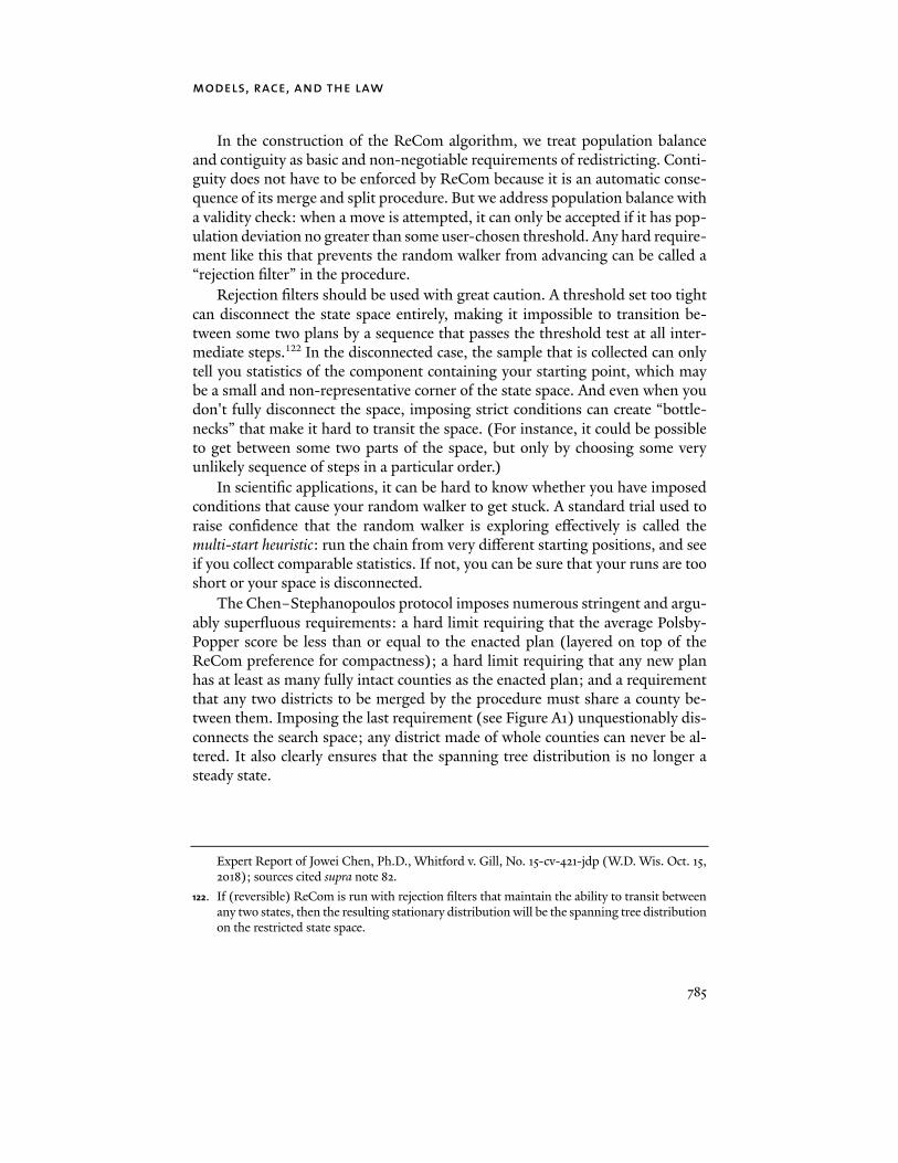
models, race, and the law
785
In the construction of the ReCom algorithm, we treat population balance and contiguity as basic and non-negotiable requirements of redistricting. Conti-guity does not have to be enforced by ReCom because it is an automatic conse-quence of its merge and split procedure. But we address population balance with a validity check: when a move is attempted, it can only be accepted if it has pop-ulation deviation no greater than some user-chosen threshold. Any hard require-ment like this that prevents the random walker from advancing can be called a “rejection filter” in the procedure.
Rejection filters should be used with great caution. A threshold set too tight can disconnect the state space entirely, making it impossible to transition be-tween some two plans by a sequence that passes the threshold test at all inter-mediate steps.122 In the disconnected case, the sample that is collected can only tell you statistics of the component containing your starting point, which may be a small and non-representative corner of the state space. And even when you don't fully disconnect the space, imposing strict conditions can create “bottle-necks” that make it hard to transit the space. (For instance, it could be possible to get between some two parts of the space, but only by choosing some very unlikely sequence of steps in a particular order.)
In scientific applications, it can be hard to know whether you have imposed conditions that cause your random walker to get stuck. A standard trial used to raise confidence that the random walker is exploring effectively is called the multi-start heuristic: run the chain from very different starting positions, and see if you collect comparable statistics. If not, you can be sure that your runs are too short or your space is disconnected.
The Chen–Stephanopoulos protocol imposes numerous stringent and argu-ably superfluous requirements: a hard limit requiring that the average Polsby-Popper score be less than or equal to the enacted plan (layered on top of the ReCom preference for compactness); a hard limit requiring that any new plan has at least as many fully intact counties as the enacted plan; and a requirement that any two districts to be merged by the procedure must share a county be-tween them. Imposing the last requirement (see Figure A1) unquestionably dis-connects the search space; any district made of whole counties can never be al-tered. It also clearly ensures that the spanning tree distribution is no longer a steady state.
Expert Report of Jowei Chen, Ph.D., Whitford v. Gill, No. 15-cv-421-jdp (W.D. Wis. Oct. 15, 2018); sources cited supra note 82.
122. If (reversible) ReCom is run with rejection filters that maintain the ability to transit between any two states, then the resulting stationary distribution will be the spanning tree distribution on the restricted state space.

the yale law journal forum March 8, 2021
786
FIGURE A1. code snippet: counties123
In addition, they choose a very high subsampling parameter, waiting for 10,000 accepted steps before adding any new plan to the ensemble. Subsampling is essential for MCMC methods invoking physics-inspired techniques like tem-perature variation, as in the past redistricting work of Mattingly and Imai,124 because it skips over “hot” plans that may not pass the validity requirements. But we know of no argument for subsampling with a ReCom chain, where all plans pass validity checks. In this setting, subsampling needlessly throws information away. To quote from the Handbook of MCMC, “Subsampling cannot improve the accuracy of MCMC approximation; it must make things worse.”125
To summarize the most serious problems we find with Article's sampling protocol:
• Overzealous subsampling (every 10,000th map) leads to samples
that are far too small (1000) to estimate a full distribution. • Numerous rejection conditions (e.g., Polsby-Popper, intact coun-
ties) and no multi-start heuristics raise concerns of bottlenecks and disconnection.
• Only allowing merging for districts that share a county between them skews the sampling distribution in an uncontrolled manner and creates strong dependence on the initial starting point for a chain.
123. The code snippet that selects districts to be merged, which we have run through a Java for-matter for legibility. Two districts can only be merged if a county is split between them.
124. See supra note 90. 125. See Geyer, supra note 118, at 27.

models, race, and the law
787
Finally, it is not clear what the authors intended to demonstrate with the “al-ternative methodology” offered in their Appendix D. There, they present an ex-periment in which even 100 rather than 1000 points pulled from a ReCom dis-tribution will give the same median value, whether created along one long chain or 100 individual ones. If this tells us anything about the present application, it lends support to the idea that ReCom converges quickly to a stationary distribu-tion on its component of the state space. That is, assuming the individual runs were shorter than the single run, this demonstration supports the long-standing claims about the efficiency of ReCom but only amplifies, rather than assuages, worries that the random walker in the Chen–Stephanopoulous experiments might be stuck in a small component of the state space. As we will see below in Figure A5, those worries are warranted.
A.2. The Code Itself
The authors’ codebase uses a mix of R (for EI) and Java (for ensembles). As we were repeatedly reminded during our replication work, even one line of buggy code can compromise an entire data operation. As one small indication, Figure A2 shows a minor error in their MOD definition logic. In principle, a glitch like this could throw the analysis way off, though in practice this particular error is buried in a rare case (where minority voters prefer Romney to Obama) and may have little to no impact on findings.
But what about the difficult part of the code, where the graph algorithm is implemented? Because the code is sparsely commented and the replication ma-terials come with no unit tests or examples, it becomes formidably difficult to analyze it in detail. This is even true when a high-level data team has several months to develop a replication study like the present one; now imagine a liti-gation context, where a similar codebase is turned over to opposing attorneys who have only two weeks to examine it. The chances that the code can be con-firmed to perform as advertised are essentially zero.
The MGGG Redistricting Lab offers open-source, publicly accessible imple-mentations of ReCom in Python and Julia with extensive documentation;126 the contributors and users include students, faculty, redistricting practitioners, and professional developers. This is a case in which it should be a relatively easy de-cision to use widely reviewed code with a multi-year track record rather than a homemade alternative.
126. See GitHub, supra note 72.

the yale law journal forum March 8, 2021
788
FIGURE A2. code snippet: mod 127
A.3. Running EI on Each County
In Part IV, we noted that running EI separately on each of the 254 counties in Texas might sound powerful, but is actually inadvisable because it leans into EI’s known difficulties dealing with small sub-populations. For instance, Andrews, Dawson, Martin, and Gaines are a cluster of demographically similar counties in West Texas with a combined population of around 50,000 people. It stands to reason that EI will handle them better together than individually, because there will be more varied precinct data on which to base the model inferences.
127. Code snippet to identify “minority opportunity districts,” separated and commented for read-ability. Black and Hispanic opportunity districts are defined for object “ag” (an aggregate of precinct-level vote estimates) by multivariate compound statements; in the circled expres-sions, DEMS should be replaced by REPS to match the description in the Article.

models, race, and the law
789
FIGURE A3. estimated black support for obama across texas precincts128
And, perhaps surprisingly, this particular toggle in the settings matters quite a bit. Figure A3 shows that changing from “Preferred EI” in only this way causes a huge change in the inferred Black support for Obama across precincts. Instead of estimates of precinct-level Black support for Obama uniformly near 90%, by-county runs report a significant share of precincts with 40-60% support. As a point of comparison, the 2012 Cooperative Congressional Election Survey found that support for Obama among non-Hispanic Black voters in Texas was over 90%.129
128. The estimate of Black voters’ support for Obama in each precinct as we toggle only the statewide/by-county setting for EI. The scatterplot shows the 9,082 precincts of Texas. Statewide EI, as in the “Preferred” style, reports high levels of Obama support; running the same script looped over the individual countries, as in the Article, reports a large share of precincts where Black voters are roughly evenly split between Obama and Romney, which seems fairly implausible.
129. Stephen Ansolabehere & Brian Schaffner, CCES Common Content, 2012, HARV. DATAVERSE, https://doi.org/10.7910/DVN/HQEVPK [https://perma.cc/KGR5-29U2] (vote validated dataset, variables = race, hispanic, inputstate and CC410a). Estimated support is 94.7%, with a 95% confidence interval of [90.8, 97.3] based on an exact binomial test.

the yale law journal forum March 8, 2021
790
A.4. Interpreting Criteria in Ensemble-Generation
In Part IV we discussed the impact of “turning the knobs” related to EI and use of additional statewide electoral data to define minority opportunity dis-tricts. Another crucial modeling choice centers interpreting the traditional crite-rion of respecting political boundaries, such as counties and municipalities, by trying to minimize the extent to which those units are split by district lines.
A.4.1. County-Conscious Sampling
County preservation is a reasonable priority in Texas because a correspond-ing rule is found in Article 3, § 26 of the state’s constitution. County preservation is not a named priority in several other states in the Article.130 Nevertheless, the authors implement a uniform county filter across every state. And the filter is extremely strict; we will see that it categorically blocks the random walker from making changes in most of rural Texas, so nearly all variation is in the urban counties.
There are many ways of handling county splits, and several are compared in Figure A4. We generate seven different ensembles for this figure with one mil-lion plans each, using different methods that either use weighting or rejection filters to accomplish greater county integrity. Column (1) shows an ordinary ReCom ensemble made with no attention to county lines. Column (2) imple-ments the requirement that any merged districts must share a county (as in Fig-ure 6). Column (3) implements the rejection filter that blocks new plans with even one more county split than the enacted plan. And column (4) combines both (2) and (3), as in the Article. Columns (5) and (6) use a softer method to weight in favor of county integrity: after two districts have been merged, ReCom draws a spanning tree of the double-district to cut it in two in a new way. One can assign random weights to the edges and use a fast algorithm to find a minimum spanning tree (MST). A soft way to favor county integrity is to put slightly higher random weights on the edges within counties, so that a min-imum spanning tree is likely to include between-county edges and therefore likely to divide along a county line. Column (5) shows the outcome if the within-county edges are given weights in (1.1, 2.1) while the between-county edges have weights from (1, 2); column (6) bumps the within-county weights to the (2, 3) range for a stronger effect. Finally, column (7) applies a different rejection filter, restricting the number of county pieces. That is, the intact-county filter in (3) only asks whether a county is divided, but does not measure the number of di-visions.
130. See supra notes 14-15 and accompanying text.

models, race, and the law
791
FIGURE A4. comparing county filters131
131. These are many ways of handling a county criterion. Each column shows an ensemble of 100,000 maps, counting the number of House districts with more Obama than Romney votes. Given this variability, it would be reasonable to declare that 51-57 Obama districts, or even 50-58, is the normal range. It is far less reasonable to declare 54 as the median—and

the yale law journal forum March 8, 2021
792
In large counties like Dallas County and Harris County, which are larger than a congressional district, the intact-county filter would make no distinction be-tween touching three districts or 30. The pieces filter restricts the number of fragments in the plan overall to no more than the number in the enacted plan.
Scanning the outputs, it is striking that the approaches that most skew the Obama count are the ones that impose rejection filters alone, (3) and (7), and they push the count in opposite directions. This offers a strong reminder that each state’s rules should be handled with care and reinforces a theme that emerges throughout our study of the Article's methods: graduated effects should be preferred to binary yes/no effects when dealing with matters of degree.
A.4.2. Impacts on Ensemble Geography
In Figure A5 we present a series of heatmaps that show how many times each precinct in Texas changes its district assignment across a run of one million steps with varying criteria, with yellow as the highest frequency and blue as the lowest. In the top row we run ReCom with no county filter as in Figure A4(1) and ob-serve that precincts flip to different districts across the state. In the next rows we impose the tree-weighting scheme described above, as in columns (5)–(6) from the last figure. The effects are quite visible compared to ordinary ReCom, espe-cially in North Texas where counties follow a grid pattern—now we can see whole rural counties flipping together. We note that a stronger weighting factor produces crisper county lines, but still allows widespread changes. Each of the weighting methods, like ordinary ReCom, leads to a visually indistinguishable heatmap whether the chain was run from the enacted plan or from an alternate random seed.132
Finally, we compare to ensembles created with the strict double-layered county filter just as Chen and Stephanopoulos use it in their Article (Figure A4(4), combining (2) and (3)). The results are quite stark: most of the state is completely untouched by their randomization of districts, even after a million steps, staying exactly as it was in the initial plan. The most-flipped precincts are hard to see in a map of the state because they are so concentrated in Dallas/Fort Worth, San Antonio, and Houston. And even after one million steps, the chains that were run from different initial starting points are producing visibly different patterns. This finding presents conclusive evidence that there are large areas in
declare a plan with55 such seats to “overrepresent” minorities—which would be the conclusion from the method in the Article.
132. Multiple seed plans are available in our replication materials. Models-Race-Law, GITHUB https://github.com/mggg/models-race-law [https://perma.cc/KR3G-86Y3].

models, race, and the law
793
the universe of legally valid districting plans for the Texas House that their en-sembles never visit.133
133. We confirmed that this is true for their actual ensembles used in their analysis as well as for our reconstructions of their method. Demonstrations can be found in our replication materi-als.

the yale law journal forum March 8, 2021
794
FIGURE A5. visualizing the diversity of samples134
134. Heatmap of Texas precincts, showing how many times they change district assignment over a run of one million steps. The Chen-Stephanopoulos method does not explore this effec-tively.

models, race, and the law
795
A.4.3. Municipalities
A municipality preservation rule is also imposed in the Article, again with a hard threshold. This does not match up with the ex ante rules for redistricting in Texas or in most other states in the authors’ sample. Of the nineteen states in the study, only three (AZ,135 CA,136 SC137) mention cities as such in their redis-tricting rules, and four (DE,138 IL,139 NV,140 VA141) have no rule at all regarding counties, municipalities, or any political boundaries.
The authors’ style of operationalizing municipality preservation is interest-ing enough to merit discussion. In many states, there is no authoritative source to find boundaries for relevant municipal geographies. In order to build an ap-proach across states, the authors turn to a Census data product called Census Places.142 These include not only “Incorporated Places” like cities and towns, but also “Census-Designated Places” like Native American reservations and various land use areas that are chosen by the Census Bureau, not the state, as being ap-propriate for statistical tabulation.
Figure A6 shows Census Places statewide and in a Fort Worth inset, showing that the Places can include strands and spurs and empty loops. The authors make their technique municipality-conscious in two ways, both extremely strong. One is to impose another rejection filter that requires accepted plans to have at least as many intact Places as the enacted plan. The second is a fundamental shift whose impacts are hard to understand completely. They do not build their plans
135. AZ. CONST. art. 4, pt. 2, § 1(14)(E) (“To the extent practicable, district lines shall use visible geographic features, city, town and county boundaries, and undivided census tracts.”).
136. CA. CONST. art. 21, § 2(d)(4) (“The geographic integrity of any city, county, city and county, local neighborhood, or local community of interest shall be respected in a manner that mini-mizes their division to the extent possible without violating the requirements of any of the preceding subdivisions.”).
137. 2011 Redistricting Guidelines, S.C. SENATE (Apr. 13, 2011), redistricting.scsenate.gov /Documents/RedistrictingGuidelinesAdopted041311.pdf [https://perma.cc/JRV7-CHTJ]; 2011 Guidelines and Criteria for Congressional and Legislative Redistricting, S.C. HOUSE JUDICIARY
COMM., redistricting.schouse.gov/6334-1500-2011-Redistricting-Guidelines-(A0404871).pdf [https://perma.cc/FAC5-NY72].
138. See supra note 14.
139. See supra note 15. 140. Justin Levitt, Nevada, ALL ABOUT REDISTRICTING (2020), redistricting.lls.edu/state/nevada
[https://perma.cc/DV4T-ZAW3]. 141. Justin Levitt, Virginia, ALL ABOUT REDISTRICTING (2020), redistricting.lls.edu/state/virginia
[https://perma.cc/V846-AHEP]. 142. Census Places are described in Chapter 9 of the Geographic Areas Reference Manual. U.S.
CENSUS BUREAU, GEOGRAPHIC AREAS REFERENCE MANUAL ch. 9 (2020), www2.census.gov /geo/pdfs/reference/GARM/Ch9GARM.pdf [https://perma.cc/7XSW-J6HE].

the yale law journal forum March 8, 2021
796
out of whole precincts, as we do in our replication runs. Instead, they create novel geographic units that they call “base polygons,” defined as intersections of block groups and Places.
These choices—new building blocks, yet another rejection filter—certainly could have a major impact on the findings, and they are not justified in the Arti-cle or well-tailored to state law.
We stand to learn a great deal from continued investigations that meet the highest standards of data science while staying grounded in the details and the meaning of the law. FIGURE A6.143 census places
Moon Duchin is Associate Professor of Mathematics; Director of the Program in Sci-ence, Technology, and Society; and Senior Fellow in the Tisch College of Civic Life at Tufts University. Email: [email protected]. Douglas M. Spencer is Professor of Law & Public Policy, University of Connecticut and Distinguished Faculty Fellow (2020-2021) at the Byron R. White Center for the Study of American Constitutional Law at the University of Colorado, Boulder. Email: [email protected]. We are grateful to Amariah Becker, Guy-Uriel Charles, Miguel de Figueiredo, Chris Elmendorf, Dara Gold, Sam Hirsch, Dan Ho, Tyler Jarvis, Ellen Katz, Vlad Kogan, Justin Levitt, Sachin Pandya, Kevin Quinn, Michael Ratcliffe, Bertrall Ross, and Peter Siegelman for their helpful input and feedback. We are also indebted to Anna Dorman,
143. Left: places in shapefile Texas. Right: a close up of the Fort Worth area.

models, race, and the law
797
Parker Rule, Gabe Schoenbach, Jackson Skeen, and Matthew Sun for their excellent research assistance.