Wireless Channel Models

8- 1

Why do we need models?

Help analyze the performance of large systemsAsk fundamental questions about a system

E.g. what is the best I can do with a given system?Allows comparison of two or more systemsCaveats:

Less accurate compared to experimentation and simulationEvery model makes assumptionsResults obtained using a model must be validated against reality

Wireless Channel Models: Outline

We want to understand how wireless channel parameters such as

Carrier frequencyBandwidthDelay spreadDoppler spreadMobile speed

affect how a channel behaves from a communication system point of viewStrategy: start with physical models and end with statistical models

Slides used in this class is based on material from Chapter 2 of Tse& Viswanath and from presentations by David Tse

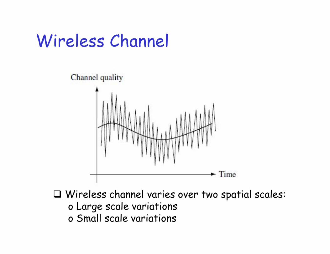
Wireless Channel

Wireless channel varies over two spatial scales:o Large scale variationso Small scale variations

Free Space, fixed Tx Antenna

Consider a fixed Tx antenna in free spaceElectric far field at time t:

(r, , ) is the point u in space where field is measuredf: carrier frequency, c: speed of lightr: distance between point u and antennas( , ,f) radiation pattern of sending

antenna

rcrtff

rtfE sr

)/(2cos),,(),,(,,

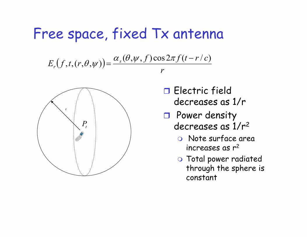
Free space, fixed Tx antenna

Electric field decreases as 1/rPower density decreases as 1/r2

Note surface area increases as r2

Total power radiated through the sphere is constant

tP

r

rcrtff

rtfE sr

)/(2cos),,(),,(,,

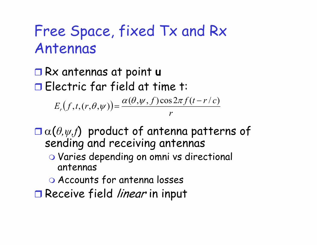
Free Space, fixed Tx and Rx Antennas

Rx antennas at point uElectric far field at time t:

( , ,f) product of antenna patterns of sending and receiving antennas

Varies depending on omni vs directional antennasAccounts for antenna losses

Receive field linear in input

rcrtff

rtfEr)/(2cos),,(),,(,,

Free Space, Moving Antenna

Consider now a receiver Rx is moving away from Tx with velocity v

Initially at r0; r(t) = r0 + vtElectric field at Rx at time t:

Received sinusoid has frequency f(1 �– v/c)!o Doppler shift = -fv/c

vtrcrtcvff

vtrcvtcrtff

vtrtfEr

0

0

0

00

)/)/1((2cos),,(

)//(2cos),,(),,(,,

Phase difference between two waves

Odd multiple of destructive interferenceEven multiple of constructive interference

Reflecting wall, fixed antenna

Assume static Rx; perfectly reflecting wallRay tracing model

Assumption: received signal superposition of two waves

rdcrdtf

rcrtf

tfEr 2)/)2((2cos)/(2cos,

)(42)2(2rd

cf

cfr

crdf

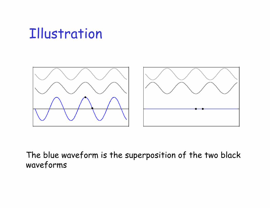
Illustration

The blue waveform is the superposition of the two black waveforms

Coherence distance

Coherence distance is distance from peak to valley

xc = /4Distance over which signal does not change appreciably

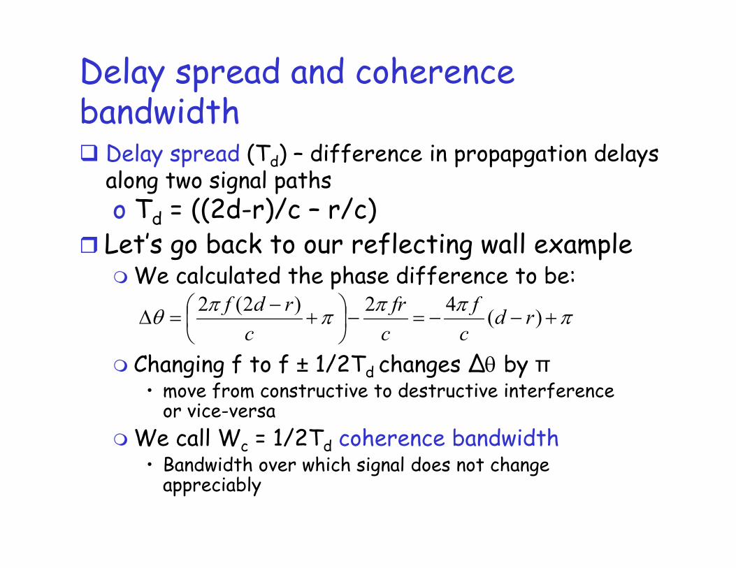
Delay spread and coherence bandwidth

Let�’s go back to our reflecting wall exampleWe calculated the phase difference to be:

Changing f to f ± 1/2Td changes by �• move from constructive to destructive interference

or vice-versaWe call Wc = 1/2Td coherence bandwidth

�• Bandwidth over which signal does not change appreciably

Delay spread (Td) �– difference in propapgation delays along two signal pathso Td = ((2d-r)/c �– r/c)

)(42)2(2rd

cf

cfr

crdf

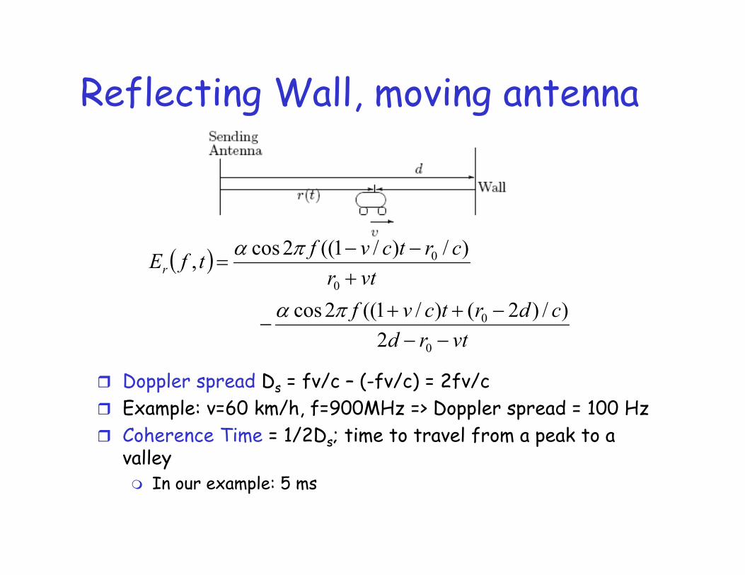
Reflecting Wall, moving antenna

Doppler spread Ds = fv/c �– (-fv/c) = 2fv/cExample: v=60 km/h, f=900MHz => Doppler spread = 100 HzCoherence Time = 1/2Ds; time to travel from a peak to a valley

In our example: 5 ms

vtrdcdrtcvf

vtrcrtcvf

tfEr

0

0

0

0

2)/)2()/1((2cos

)/)/1((2cos,

Doppler Shift Effect

Assume mobile very close to the walld ~ r0 + vt

vtrdcdrtcvf

vtrcrtcvf

tfEr

0

0

0

0

2)/)2()/1((2cos

)/)/1((2cos,

vtrcdtfcdrcvtf

tfEr0

0 )/(2sin)/)(/(2sin2,

Reflecting Wall, moving antenna

Multipath fading: Moving between constructive and destructive interference of two waves

Once every 5 msSignificant changes in path length (denominator) occur on time scales of several seconds or minutes

Summary

We applied physical model in a toy example to understand multipath fading in terms of:

Delay spread & Coherence bandwidthDoppler spread & Coherence time

But, we want to model a wireless channel in a world with many obstacles, reflectors etc.We are more interested in aggregate behavior of channel

Not so much detailed response on each path

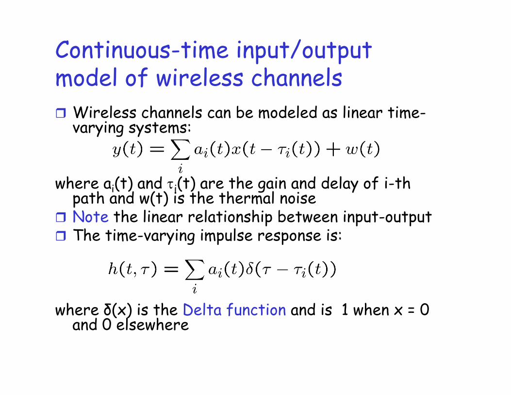
Continuous-time input/output model of wireless channels

Wireless channels can be modeled as linear time-varying systems:

where ai(t) and i(t) are the gain and delay of i-th path and w(t) is the thermal noiseNote the linear relationship between input-outputThe time-varying impulse response is:

where (x) is the Delta function and is 1 when x = 0 and 0 elsewhere

Continuous-time input/output models of wireless channels

In terms of time-varying impulse response, y(t) can be expressed as:

In practice, we convert a continuous time signal of bandwidth W at passband too a baseband signal of bandwidth W/2; ando Take samples at integer multiples 1/W (sampling theorem)

Discrete Time input/output model

Discrete-time (sampled) channel model:

where hl is the l-th complex channel tap.

and the sum is over all paths that fall in the delay bin

System resolves the multipaths up to delays of 1/W .

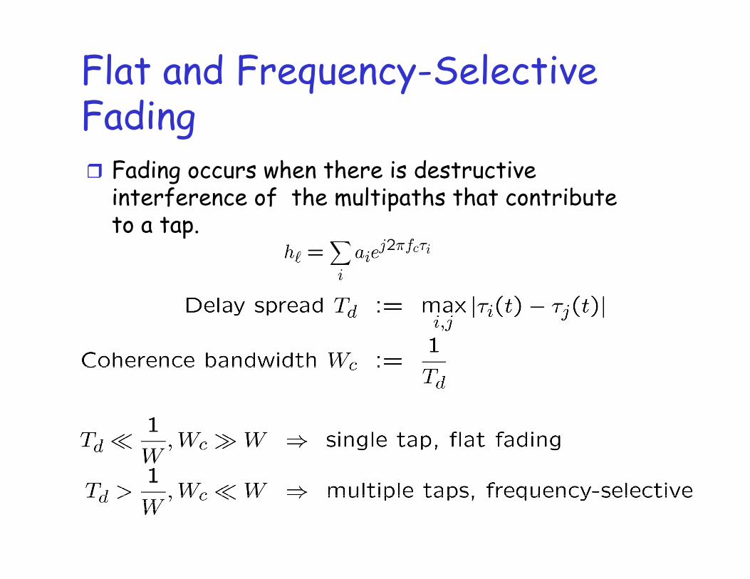
Flat and Frequency-Selective Fading

Fading occurs when there is destructive interference of the multipaths that contribute to a tap.

The channel as seen by the communication system depends on:

o Physical environment (in terms of delay spread)o Communication bandwidth

Time Variations

fc i�’(t) = Doppler shift of the i-th path

Types of Channels

Statistical Models

Consider the l-th complex channel tap

To completely specify h, we need to know each path that contributes to the tap

In practice, this is difficultWe are only interested in the sum of all the paths at each tap

When there are many reflectors in environmentMany many paths between transmitter and receiverMany many paths contributing to each channel tap

Central Limit Theorem

Sum of large number of iid random variables converges (in distribution) to the Gaussian

Complex channel tap modeled as a complex Gaussian random variable

�• This is the Rayleigh fading model

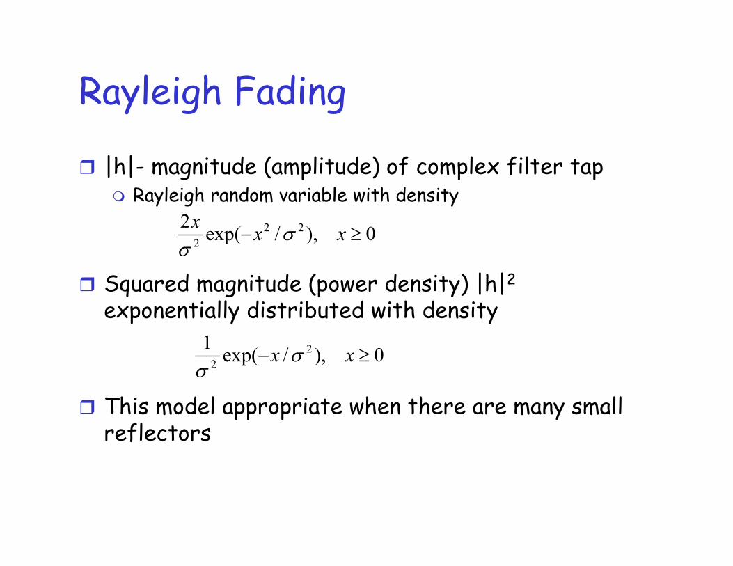
Rayleigh Fading

|h|- magnitude (amplitude) of complex filter tapRayleigh random variable with density

Squared magnitude (power density) |h|2

exponentially distributed with density

This model appropriate when there are many small reflectors

0),/exp(2 222 xxx

0),/exp(1 22 xx

Rician Fading

Appropriate when there is a large line of sight path as well as independent pathsOften more accurate than Rayleigh model

Pdf does not have a simple form and not easy to work withHas found limited applicability in research community

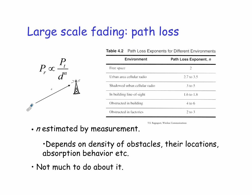
Large scale fading: path loss

tr n

PP

d

�• n estimated by measurement.

�•Depends on density of obstacles, their locations, absorption behavior etc.

�• Not much to do about it.

d

T.S. Rappaport, Wireless Communications

Shadowing

d

�• Same distance, different power. Due to shadowing.

�• Modeled as a random power distribution (log-normal)

�• Capture randomness in environment

2

52

25 14

5

t

r

dnP

d dBP

dB

Example:

Fading and Diversity

Improve performance of wireless systems by transmitting symbols over multiple paths that fade independently

Reliable communication possible as long as at least one �“strong�” path existsThis technique is called Diversity

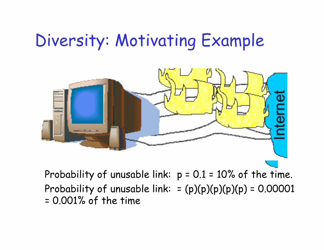
Diversity: Motivating Example

Probability of unusable link: p = 0.1 = 10% of the time.Probability of unusable link: = (p)(p)(p)(p)(p) = 0.00001 = 0.001% of the time

Wireless Channel

The channel is dynamic and it is a function of time.The reliability of the link depends upon the �“gain�” of the channel, which is a random variable always less than one.

�• Cellular LinkBuildingsCountryside

�• Wireless LANCustomers/BaristasTraffic

Three Types of Diversity

Time DiversitySpace Diversity

1. Antenna Arrays2. MIMO Systems

Frequency Diversity1. WiFi2. Cell Phones

All forms of diversity have their pros and cons.

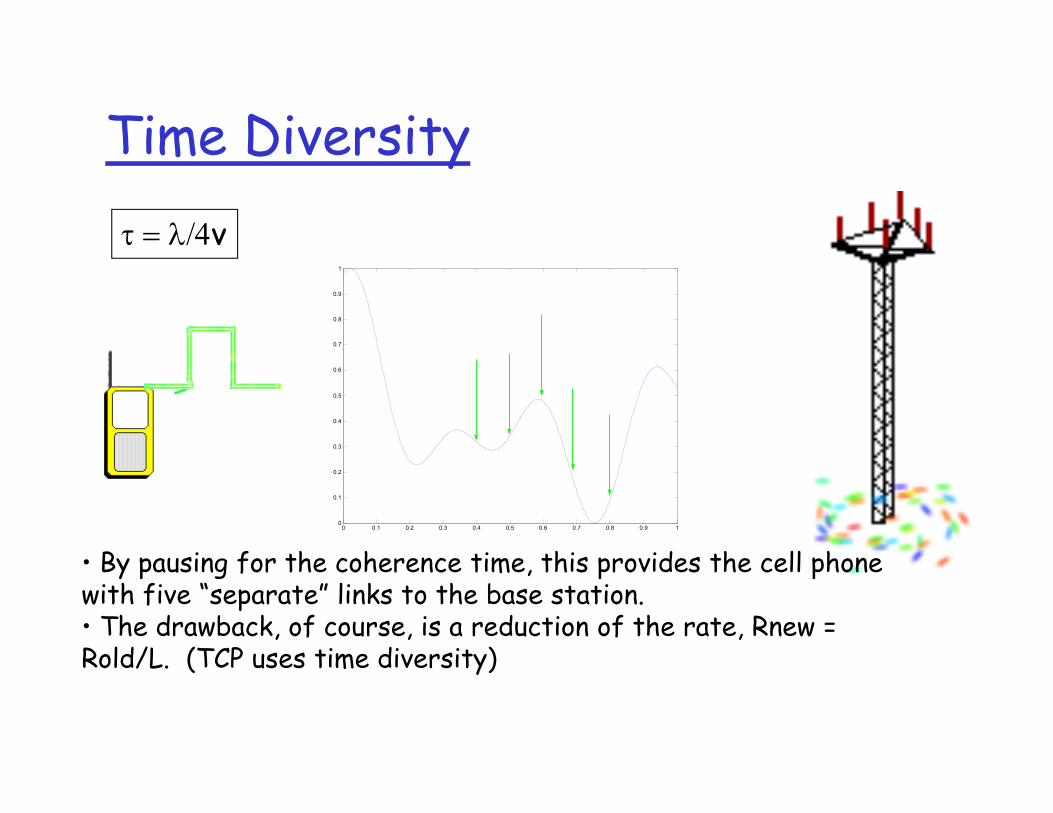
Time Diversity

0 0.1 0.2 0.3 0.4 0.5 0.6 0.7 0.8 0.9 10

0.1

0.2

0.3

0.4

0.5

0.6

0.7

0.8

0.9

1

0 0.1 0.2 0.3 0.4 0.5 0.6 0.7 0.8 0.9 10

0.1

0.2

0.3

0.4

0.5

0.6

0.7

0.8

0.9

1

0 0.1 0.2 0.3 0.4 0.5 0.6 0.7 0.8 0.9 10

0.1

0.2

0.3

0.4

0.5

0.6

0.7

0.8

0.9

1

�• All the obstacles between the cell phone to base station is modeled by a channel gain, h(t).�• This includes the mobility of the phone/user.

Time Diversity

0 0.1 0.2 0.3 0.4 0.5 0.6 0.7 0.8 0.9 10

0.1

0.2

0.3

0.4

0.5

0.6

0.7

0.8

0.9

1

�• Receiver and Transmitter protocol states that each bit will be transmitted L times. (called repetition coding)�• Important that the coherence time of the channel elapses before retransmitting.

0 0.1 0.2 0.3 0.4 0.5 0.6 0.7 0.8 0.9 10

0.1

0.2

0.3

0.4

0.5

0.6

0.7

0.8

0.9

1

Time Diversity

0 0.1 0.2 0.3 0.4 0.5 0.6 0.7 0.8 0.9 10

0.1

0.2

0.3

0.4

0.5

0.6

0.7

0.8

0.9

1

�• By pausing for the coherence time, this provides the cell phone with five �“separate�” links to the base station.�• The drawback, of course, is a reduction of the rate, Rnew = Rold/L. (TCP uses time diversity)

v

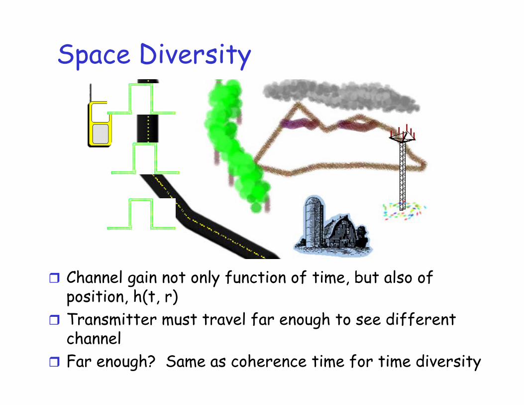
Space Diversity

Channel gain not only function of time, but also of position, h(t, r)Transmitter must travel far enough to see different channel Far enough? Same as coherence time for time diversity

Space Diversity

0 1 2 3 4 5 6 7 8 9 100

0.1

0.2

0.3

0.4

0.5

0.6

0.7

0.8

0.9

1

h1(t)

h2(t)

0 1 2 3 4 5 6 7 8 9 100

0.1

0.2

0.3

0.4

0.5

0.6

0.7

0.8

0.9

1

h1(t)

h2(t)

�• Most cell towers have multiple transmit cells serving one cell�• Down link channel - MISO system.�• Antennas must be spaced at least /2 apart to see �“independent�” channels.

Far Enough = /2

Space Diversity

Multiple antennas at phone, base station - MIMO systemCost is receiver/transmitter complexityBenefit - BER approximately 1/SNRL

0 1 2 3 4 5 6 7 8 9 100

0.1

0.2

0.3

0.4

0.5

0.6

0.7

0.8

0.9

1

h1(t)

h2(t) h3(t)

h4(t)

Probability all four channels in deep fade much smaller than probability any one channel in deep fade.

Frequency Diversity

Channel gain is a function of frequency as well, h(t,r,f)Different frequencies see different channels, this provides independent links.For example:

AM: 535-1605 kHzFM: 88-108 MHzUHF TV: 470-890 MHzCell Phones:WiFi: 2.4 �– 2.485 GHzGPS:Cloud Radar: > 30 GHz

Frequency Diversity

If signal does not reach the base station, try:�• Transmitting different frequency, at least coherence bandwidth away

Conclusion

Physical models of wireless channelsGood for preliminary understanding of fading Hard to study real-world systems

Input/Output modelsWireless channel as LTV system

Statistical modelsRayleigh and Rician models

DiversityTime �– Transmit at different times.Space �– Transmit at different points in space.Frequency �– Transmit at different frequencies, or over a bandwidth of frequencies.